Article

Arboreal Urban Cooling Is Driven by Leaf Area Index, Leaf Boundary Layer Resistance, and Dry Leaf Mass per Leaf Area: Evidence from a System Dynamics Model

by
Harold N. Eyster
1,2,* and
Brian Beckage
1,2
1
Gund Institute for Environment, University of Vermont, Burlington, VT 05405, USA
2
Department of Plant Biology, University of Vermont, Burlington, VT 05405, USA
*
Author to whom correspondence should be addressed.
Atmosphere 2023, 14(3), 552; https://doi.org/10.3390/atmos14030552
Submission received: 7 February 2023 / Revised: 25 February 2023 / Accepted: 3 March 2023 / Published: 14 March 2023
(This article belongs to the Special Issue New Approaches to Complex Climate Systems)

Abstract

:
Heat waves are becoming more frequent due to climate change. Summer heat waves can be particularly deadly in cities, where temperatures are already inflated by abundant impervious, dark surfaces (i.e., the heat island effect). Urban heat waves might be ameliorated by planting and maintaining urban forests. Previous observational research has suggested that conifers may be particularly effective in cooling cities. However, the observational nature of these studies has prevented the identification of the direct and indirect mechanisms that drive this differential cooling. Here, we develop a systems dynamics representation of urban forests to model the effects of the percentage cover of either conifers or broadleaf trees on temperature. Our model includes physiological and morphological differences between conifers and broadleaf trees, and physical feedback among temperature and energy fluxes. We apply the model to a case study of Vancouver, BC, Canada. Our model suggests that in temperate rainforest cities, conifers may by 1.0 °C cooler than broadleaf trees; this differential increases to 1.2 °C when percentage tree cover increases from 17% to 22% and to 1.7 °C at 30% cover. Our model suggests that these differences are due to three key tree traits: leaf area index, leaf boundary layer resistance, and dry mass per leaf area. Creating urban forests that optimize these three variables may not only sequester CO2 to mitigate global climate change but also be most effective at locally minimizing deadly urban heat waves.

1. Introduction

Heat waves are becoming more frequent due to climate change [1]. More frequent heat waves are especially harmful in cities because temperatures are already inflated by abundant impervious, dark surfaces (i.e., the heat island effect); air quality may often be low; and there are many vulnerable city residents [2,3,4,5]. High urban temperatures can lead to direct human and non-human animal deaths [6]. In summer 2021, a heat wave associated with anthropogenic climate change [7] on the Pacific coast of North America broke Canada’s temperature record and was associated with quadrupled human mortality [8]. Heat waves can also cause indirect effects [9], such as wildfires [10]. As climate change intensifies, ameliorating urban heat waves is becoming urgent [11,12].
The intensity of urban heat waves might be lessened by planting and maintaining urban forests [13,14,15]. Trees cool cities in multiple ways, including via evapotranspiration [16] and by blocking solar radiation from reaching the ground [17]. In addition to cooling locally, trees may also cool globally as part of efforts to sequester carbon dioxide [18,19]. Trees may be key to simultaneously tackling heatwaves at local and global scales.
Previous observational research has suggested that conifers may be particularly effective in cooling cities when compared with broadleaf trees in temperate [20] and Mediterranean climates [21]. This increased cooling capacity may be due to a variety of tree characteristics, such as leaf area index and evapotranspiration rate [21,22,23,24]. Yet the observational nature of these studies hampers identification of the key arboreal characteristics that drive cooling in cities.
Physical urban temperature models could help identify the key cooling characteristics of trees. Yet despite the documented variability across tree types, urban temperature models have not yet accounted for this variability in tree physiognomy (e.g., [25,26,27,28]).
Here, we leverage the modeling tool Stella to build a systems dynamics model of urban temperature associated with different percentage cover of either conifers or broadleaf trees. Our model includes measured physiological and morphological differences between conifers and broadleaf trees and physical feedbacks among temperature and heat fluxes. Our objective is to use this model to identify the tree traits that create differences in urban cooling.
We analyze the model in a case study of Vancouver, BC, Canada, which both has experienced high heat wave mortality [6,8] and has plans to increase its tree cover from 17% to 22% by 2050 [29]. Currently, approximately 22% of the city’s urban forest is coniferous, based on data from Metro Vancouver [30] (see Figure 1). Vancouver is a large city (>600,000 residents) in the extreme southwest of Canada with warm wet winters and moderate dry summers. Streets are forested primarily by non-native broadleaf deciduous trees [31], while native forests consist mostly of conifers, including Douglas fir (Pseudotsuga menziesii), western hemlock (Tsuga heterophylla), and western red cedar (Thuja plicata [32]. Studies have shown a large heat island effect in the city (up to 11.6 °C; [3]), as well as a park cooling effect of 1–5 °C extending outward from city parks [33]. These effects are most important in the summer, when high temperatures can lead to mortality. We expect that urban temperatures will be lower when forested with conifers and that this effect will increase as the forest cover increases. Moreover, we expect that a few conifer traits will drive this temperature difference. This study may help inform what trees Vancouver and other cities can plant and maintain in order to ameliorate heat waves.

2. Materials and Methods

2.1. System Dynamics Model

We built a system dynamics model of the heat exchange and feedback among trees and the city using Stella Architect version 2.1.5 (2629) (ISEE Systems, Lebanon, NH, USA). Stella Architect is a widely used system dynamics modeling tool that can capture the multiple feedback loops within complex physical systems [34,35]. We included heat fluxes from solar radiation, longwave radiation, conduction, convection, and evapotranspiration among air, ground, built environment, and trees (Figure 2). Rural air is assumed to be unaffected by the urban heat island and such cool air interfacing with urban air is key way that natural landscapes cool cities. We treated the built environment and tree heating mechanisms in separate modules. The model was run separately with two sets of parameters: one set of parameters represented evergreen, needle-bearing conifers (signified below by “(conifer)”) and the other broadleaf, deciduous angiosperms (signified below by “(broadleaf)”). This structure enabled comparison of heat exchange and temperature between conifers and broadleaf trees. We included variables and interdependencies that are likely to affect tree and city temperatures [36,37].
All calculations were carried out on a per-area basis. The modeled timeframe was set to 6 d (144 h) in order to provide sufficient time to overcome the initial temperature condition. All visualizations and model inference was based on the last 24 h of the timeframe (i.e., 120–144 h). Rather than setting the sum of fluxes equal to zero and solving for the equilibrium temperature [25], we solved for the dynamic, instantaneous temperature using differential equations. We used Euler integration and a time step of 1 min (DT = 1/60) to solve the differential equations. To verify that this numerical simulation was robust, we tested an integration time of 1 s (DT = 1/3600) and the Runge–Kutta 4 (RK4) integration method and achieved identical results. After creating the model, we conducted a sensitivity analysis, varying the tree parameters to identify which conifer–broadleaf differences were most important in driving differences in temperature.
Parameter values were set to values representative of 1 August in Vancouver, BC (Table 1), including the current urban forest cover of 17%, target 2050 forest cover of 22% [29], and 30%. The first author lived for five years in this region, and their first-hand experiences of how temperature varied near different urban trees motivated the conceptualization of this study.

2.1.1. Module 1: Built Environment Model

The temperature of the built environment, T b u i l t , was initialized at 22 °C. Change in T b u i l t is driven by heat fluxes into and out of the built environment:
Δ T b u i l t C = q s o l . b + q r a d . b q c o n v . b q c o n d ,
where C is the heat capacity of the built environment (J/m 2 /K), q s o l . b is the solar heat flux entering the built environment (J/m 2 /h), q r a d . b is the net longwave radiation entering the built environment (J/m 2 /h), q c o n v . b is the net convection heat flux exiting the built environment (J/m 2 /h), and q c o n d is the net conduction heat flux exiting from the built environment into the ground (J/m 2 /h). The ground is assumed to be a uniform dirt-like material that is representative of the average underlying substrate across the city.
C = C v H ,
where C v is the volumetric heat capacity of the built environment (J/m 3 /K) [38] and H is its effective height (m).
q s o l . b = q e x t + q s o l . b . a ,
q s o l . b . a = ( 1 α b ) ( 1 g ) s n I ,
where q e x t (J/m 2 /h) is the solar irradiance that goes through the tree canopy to the built environment below (see Equation (19)); q s o l . b . a is the solar irradiance directly entering the built environment; α b is the albedo of the built environment, i.e., the fraction of solar radiation reflected by the built environment (dimensionless); g is the fraction of the built environment covered by trees (dimensionless); s is the number of seconds in an hour (to convert the quantity from J/s to J/h); and I is the direct normal irradiance (DNI; J/m 2 normal to the sun per second) taken from the Physical Solar Model (PSM3) of the National Solar Radiation Database (NSRDB; https://nsrdb.nrel.gov/data-viewer; accessed on 24 May 2022) [52] for 1 August 2020 in Vancouver, BC (location ID = 262013). We chose this date because it is, on average, the hottest day of the year (https://weatherspark.com/m/476/8/Average-Weather-in-August-in-Vancouver-Canada; accessed on 22 January 2021). The same direct normal irradiance values are used for each of the six model run days. n is the proportion of the direct normal irradiance that is incident onto a square meter tangent to the earth (dimensionless) and is approximated by
n = sin ( 1 3.82 ( t t s ) ) cos ( L δ ) ,
where t is time (h) since the start of the model run (set to midnight) and t s is the time of sunrise (h). L is the latitude and δ is the declination angle. All angles are measured in radians. δ is given by
δ = 23.45 2 π 360 sin ( 2 π 284 + D 365 ) ,
where D is the day of year (d).
q r a d . b = q r a d . g e 2 q r a d . b . a ,
q r a d . b . a = ϵ b σ s T b u i l t 4 ,
where q t r e e . g e is the longwave radiation emitted by the trees (J/m 2 /h; divided by two because only half of the emitted radiation reaches the built surface). ϵ b is the emissivity of the built environment, and σ is the Stefan–Boltzmann constant (W/m 2 /K 4 ).
q c o n v . b = q c o n v . b . a + q c o n v . b . u ,
where q c o n v . b . a is the convection heat flux from the built environment to the rural air and q c o n v . b . u is the convection heat flux between the built environment and the air beneath the trees.
q c o n v . b . a = s ( 1 g ) h ( T b u i l t T a i r ) ,
where h is the urban convective heat transfer coefficient (J/K/s) and T a i r is the temperature of the rural air (°C) and serves as the heat sink above the modeled region [26].
Following Silva et al. [26] and Rowley and Eckley [53],
h = 11.8 + 4.2 v ,
where v is the wind velocity.
T a i r = T a i r . h i g h T a i r . l o w 2 sin 1 3.82 ( t t s ) π 2 + T a i r . h i g h + T a i r . l o w 2
approximates the daily oscillation between the low rural air temperature ( T a i r . l o w , °C; experienced at sunrise) and the high rural air temperature ( T a i r . h i g h , °C; experienced in the afternoon). All angles are in radians.
q c o n v . b . u = g h ( T b u i l t T u n d e r s t o r y ) .
Because air at the built–tree interface would be similar to the tree temperature, T u n d e r s t o r y (°C) is approximated by the leaf temperature, T t r e e (°C).
q c o n d = k g s ( T b u i l t T g ) d ,
where k g is the thermal conductivity of the ground (W/m/K), d is the ground depth (m), and T g is the temperature (°C) of the ground at depth d and serves as the heat sink below the modeled region, following Pace et al. [25].

2.1.2. Module 2: Tree Model

The temperature of the urban forest, T t r e e was initialized at 22 °C. Change in T t r e e was driven by heat fluxes into and out of the tree canopy:
Δ T t r e e C g g = q s o l . g q e v a p + q r a d . g q c o n v . g ,
where C g is the heat capacity of leaves (J/m 2 /K), q s o l . g is the solar heat flux (J/m 2 /h), q e v a p is the heat loss through evapotranspiration (J/m 2 /h), q r a d . g is the net longwave radiation (J/m 2 /h), and q c o n v . g is the net convection heat flux (J/m 2 /h) [25,26].
C g = m a L A I 1 f w ( ( 1 f w ) c d r y + ( f w c w a t e r ) ) ,
where, following Equations (10) and (11) in [39], m a is the dry leaf mass per unit leaf area (kg/m 2 ), L A I is the leaf area index, f w is the fraction of the leaf that is water (dimensionless), c d r y is the specific heat of dry leaf biomass (J/kg/K), and c w a t e r is the specific heat of water (J/kg/K).
q s o l . g = q d i r e c t q e x t ,
where q d i r e c t is the sunlight energy that enters the trees (J/m 2 /h) and q e x t is the sunlight energy that passes through the canopy and enters the built environment beneath.
q d i r e c t = L A I × ( 1 α g ) g s n I ( 1 ϵ c ) ,
where α g is the albedo of the leaves (dimensionless) and ϵ c is the photosynthetic efficiency of the leaves [42].
q e x t = q d i r e c t e K × L A I ,
where K is the extinction coefficient (dimensionless) according to the Beer–Lambert law [43].
q r a d . g = g q r a d . b . a q r a d . g e ,
q r a d . g e = 2 × L A I × ϵ g σ s g T t r e e 4 ,
where q r a d . b . a is given in Equation (8) and ϵ g is the emissivity of the leaves (dimensionless).
q e v a p = E h v g ,
where E is the evapotranspiration rate (kg/m 2 /h) and h v is the latent heat of vaporization of water (J/kg).
E = C l e a f C a i r r t o t L A I × s ,
where C l e a f is the water vapor concentration at the evaporating surface within the leaf (kg/m 3 ), C a i r is the water vapor concentration in the air (kg/m 3 ), and r t o t is the total resistance (s/m) [36].
Equation (23) assumes that higher leaf area index causes an increase in total evapotranspiration, which has been widely demonstrated in the literature [37,54]. Although there may be slightly lower per-leaf evapotranspiration at higher L A I values [37], we use a simple linear relationship. Other studies have mistakenly applied a per-leaf decrease in evapotranspiration to the whole tree and treated L A I and E as inversely proportional for entire trees [25,55].
C l e a f = M w e s a t . l e a f R T t r e e ,
C a i r = M w e a i r R T a i r ,
where M w is the molecular weight of water (kg/mol), e s a t . l e a f is the saturation vapor pressure (Pa) of the leaf, e a i r is the vapor pressure of the air, and R is the universal gas constant (J/mol/K).
e a i r = H r 100 e s a t . a i r ,
where H r is the relative humidity (in percent) and e s a t . a i r is the saturation vapor pressure of the air (Pa).
Following the World Meteorological Guide [56], the saturated vapor pressures of the leaf and air are approximated as follows:
e s a t . l e a f = 100 × 6.112 exp 17.62 T t r e e T t r e e + 243.12 ,
e s a t . a i r = 100 × 6.112 exp 17.62 T a i r T a i r + 243.12 .
The total resistance to evapotranspiration, r t o t in Equation (23), consists of resistance through the abaxial (lower) surface of the leaf ( r t o t . a b a x i a l ; s/m) and the upper (adaxial) surface of the leaf ( r t o t . a d a x i a l ; s/m), summed in parallel [36,39]:
r t o t = r t o t . a b a x i a l r t o t . a d a x i a l r t o t . a b a x i a l + r t o t . a d a x i a l .
Because some resistances act in parallel and others in series, care must be taken in calculating the totals [39]. For the abaxixal surface, the stomatal ( r s t o m a t a l . a b a x i a l ; s/m) and intracellular resistances ( r i n t r a c e l l u l a r . a b a x i a l ; s/m) are added in series, and the resultant quantity is added in parallel with the cuticular resistance ( r c u t i c u l a r . a b a x i a l ; s/m) [36]. This resultant quantity is then added in series with the boundary-layer resistance ( r a i r . a b a x i a l ; s/m) [36]:
r t o t . a b a x i a l = 1 1 r c u t i c u l a r . a b a x i a l + 1 r s t o m a t a l . a b a x i a l + r i n t r a c e l l u l a r . a b a x i a l + r a i r . a b a x i a l .
The same is repeated for the adaxial surface:
r t o t . a d a x i a l = 1 1 r c u t i c u l a r . a d a x i a l + 1 r s t o m a t a l . a d a x i a l + r i n t r a c e l l u l a r . a d a x i a l + r a i r . a d a x i a l .
Wind decreases the boundary layer resistance more for thin needles than larger broad leaves [36]:
r a i r . a d a x i a l = r a i r . a b a x i a l ,
r a i r . a b a x i a l [ conifer ] = 1000 5.0 + 74.4 v ,
r a i r . a b a x i a l [ broadleaf ] = 100 0.52 + 3.2 v ,
where the conifer Equation (33) is derived from observations of Abies amabilis [57] and the broadleaf Equation (34) is derived from experiments with a synthetic broad leaf [58]. Studies have shown that even at night, tree stomata often remain open and evapotranspiration remains linked to water vapor deficit and wind speed [36], so we treat stomatal resistance as temporally constant for simplicity.
q c o n v . g = q c o n v . g . a + q c o n v . g . u ,
where q c o n v . g . a is the convection heat flux (J/h) from trees to rural air and q c o n v . g . u is the convection heat flux from the bottom layer of leaves to the air above the built environment.
q c o n v . g . a = 2 c p g s ( T t r e e T a i r ) L A I r a i r . a b a x i a l ,
where c p is the specific heat of moist air at constant pressure (J/mol/K) [39]. Because the boundary resistance is equivalent for both sides of the leaf, we use just abaxial resistance in the equation for simplicity, and double the entire convection term, following [39].
q c o n v . g . u = c p g s ( T t r e e T b u i l t . u n d e r t r e e ) 1 r a i r . a b a x i a l .
Because air at the built environment beneath the tree is likely similar to the built environment temperature, T b u i l t . u n d e r t r e e (°C) is approximated by the built environment temperature, T b u i l t (°C). We assume that only the lower surface of the bottom layer of leaves interacts with the undertree air.

3. Results

Our model results were consistent with empirical observations of tree temperature—our modeled maximum broadleaf and conifer temperatures were within 1 °C of those temperatures measured in Vancouver, BC, based on Lansdsat 8 imagery [20].
At 17% tree cover, the maximum temperature of the built environment was 1.0 °C warmer when it was forested by conifers than by broadleaf trees (Figure 3a). When tree cover increased to 22%, the temperature differential increased to 1.2 °C (Figure 3b); when tree cover increased to 30%, conifers were 1.7 °C cooler (Figure 3c).
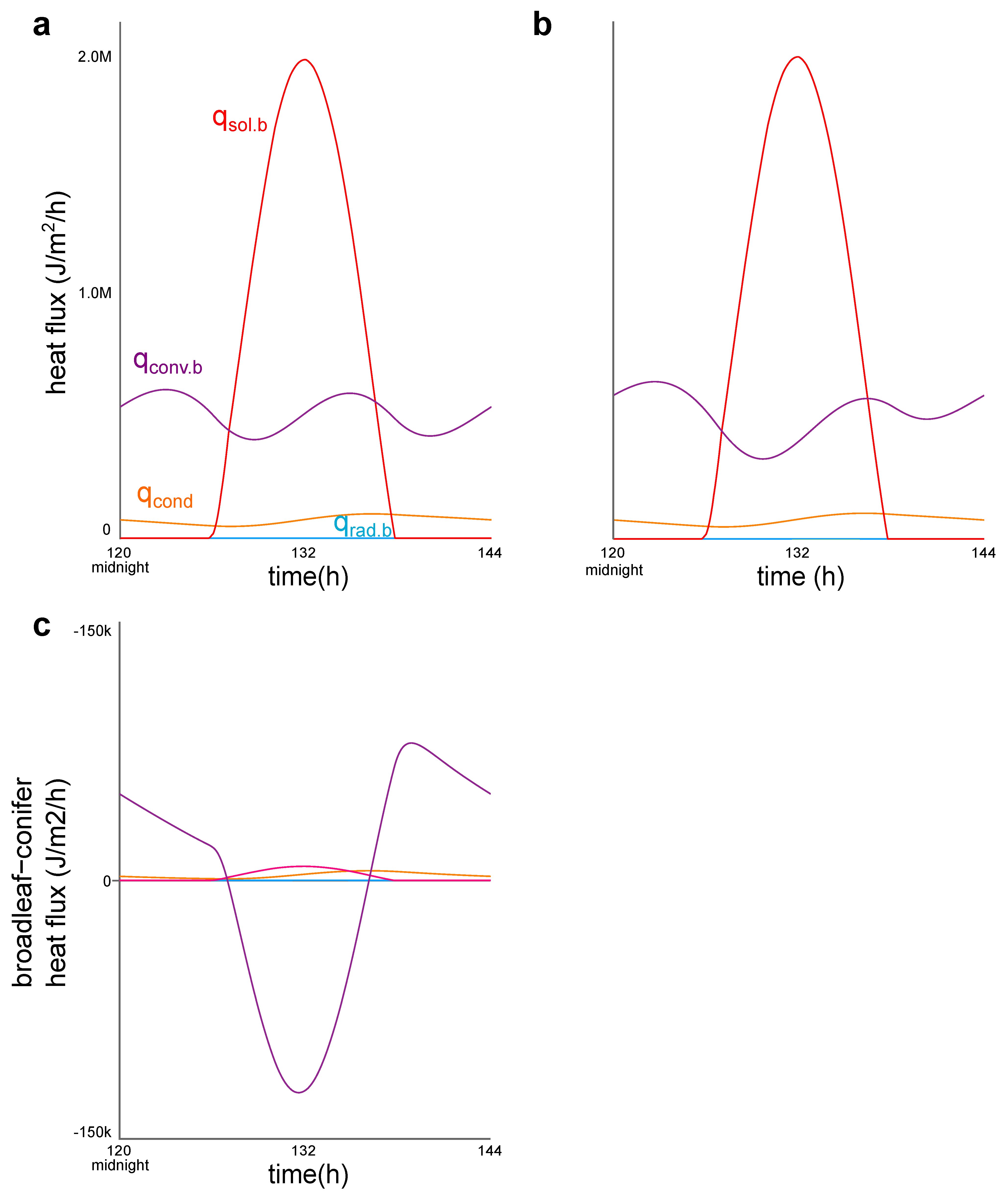
Solar radiation and convection dominated heat fluxes into and out of the built environment (Figure 4). Solar radiation was slightly higher in the broadleaf-forested built environment (because q e x t [ broadleaf ] > q e x t [ conifer ] ), and the convection heat flux was higher at night (Figure 4). Conduction also played an important role, but longwave radiation was negligible (Figure 4).
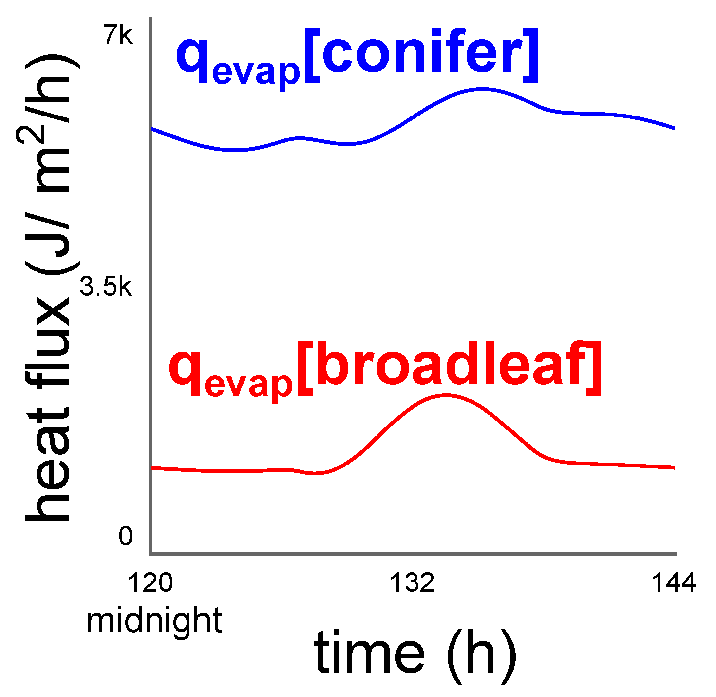
Similarly, solar radiation and convection dominated the heat fluxes into and out of the urban forests, though convection curves were shaped quite differently across the urban forest types (Figure 5). Broadleaf forests showed a single large diurnal flux of convection, while coniferous forests also showed a smaller diurnal flux and a substantial nocturnal flux. Evapotranspiration was significant in the coniferous forest, but small in the broadleaf forest (Figure 6). Longwave radiation was insignificant in both forest types (Figure 5).
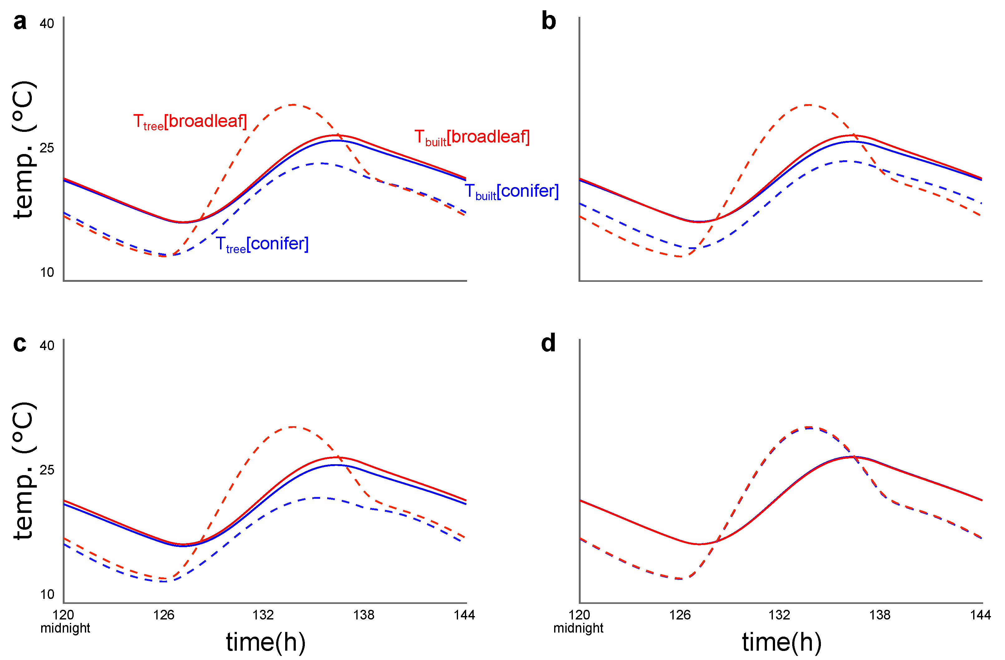
Sensitivity analysis revealed that three variables drive the conifer–broadleaf temperature differential. Setting the conifer values of leaf area index ( L A I ), leaf boundary layer resistance ( r a i r . a d a x i a l and r a i r . a b a x i a l ), and dry leaf mass per leaf area ( m a ) equal to the respective broadleaf values for these three variables removed differences between conifer and broadleaf temperatures, both for the urban forest and for the built environment (Figure 7). That is, controlling for these three variables produces equivalent temperatures for both conifer-forested cities and broadleaf-forested cities (Figure 7).

4. Discussion

This study harnessed a physical systems dynamics model of urban temperature and conifer and broadleaf tree traits to identify the degree to which conifers cool cities compared to broadleaf trees, and which key traits drive these differences. We found that conifers cool cities more than broadleaf trees and that this effect increases at higher tree cover (Figure 3). Our model suggests that this differential cooling can be fully explained by conifer–broadleaf differences in terms of three traits: leaf area index, leaf boundary layer resistance, and leaf dry mass per leaf area (Figure 7). Relative to broadleaf values, conifer values for these traits yield higher evapotranspiration, lower built environment solar radiation, and higher daytime convection, which in turn produce cooler tree and built environment temperatures (Figure 7).
Our results support the City of Vancouver’s plan to increase forest cover to 22% and its emphasis on planning native conifers such as Douglas fir (Pseudotsuga menziesii) [29], not only because they support birds [59] and mammals and help lessen flooding [60], but because they may be more effective at cooling the city.
Our finding that leaf area index is important for urban cooling is consistent with other studies (e.g., [61,62,63,64,65]). However, our leaf area index results and methods are inconsistent with physical models that assumed that single-leaf relationships between leaf area index and evapotranspiration can be applied to entire trees [25,55]. Future work might further clarify the degree to which the effect of leaf area index on evapotranspiration decays at high leaf area index values.
Our results are also consistent with a smaller body of literature on the role of boundary layer resistance in increasing evapotranspiration and lowering leaf temperature (e.g., [66,67]). Studies have often focused on stomatal resistance (or conductance) (e.g., [65,67]), but we found that boundary layer resistance was more important in cooling.
Our findings showing a negative relationship between leaf mass per leaf area and temperature are inconsistent with some studies that have shown that thick leaves are hotter [67,68]. However, the thicker leaves in these studies were likely also wider and exhibited higher leaf boundary layer resistances and lower surface-area-to-volume ratios. Thus, the particular combination of traits exhibited simultaneously by conifers appear to be uniquely important.
Beyond the conifer–broadleaf tree dichotomy, selectively planting trees that holistically exhibit high leaf area index, low leaf boundary layer resistance, and high dry leaf mass per leaf area may help cities most effectively combat increasingly frequent heat waves. Nonetheless, the cooling effect is only one of many factors that are important when considering which trees belong in a particular part of a particular city [69,70].
The three-fold greater evapotranspiration exhibited by conifers (Figure 6) is consistent with observational evidence [37], and confirms hypotheses that heightened evapotranspiration may lower conifer foliage surface temperature [20]. Moreover, the higher diurnal broadleaf tree convection suggests that, relative to conifers, broadleaf trees may warm pedestrians more and offer less respite from heat waves. When choosing to reforest or afforest cities, tree type matters.
Although strategies to mitigate high urban temperatures often focus on increasing surface albedo (e.g., [26,71]), our results suggest that strategies that increase albedo may sometimes create hotter temperatures. Specifically, our model showed that while conifers exhibit lower albedo, their higher leaf area index means that they also block more light from passing through the canopy to enter and warm the built environment below (Equation (23), Figure 4). We second Yang et al. [72] in cautioning city planners to not treat albedo as a “silver bullet”.
Studies have shown that cooling by trees varies in response to wind, moisture content, latitude, and other climate variables [15,21,33,73]. Our model is parameterized for climates, cities, and trees of the Pacific Northwest, and so our results are not necessarily indicative of conifers or broadleaf trees per se, but of the relationships among urban forests and the Pacific Northwest urban ecosystem [74]. However, our model could be extended to other regions by replacing the values from Table 1 with those relevant for a given location, and perhaps making some variables dynamic that we treated as static, and vice versa.
We included arboreal variables that are suggested to have large effects on tree temperatures. These variables proved sufficient to reproduce empirical tree temperature observations [20]. However, incorporating additional variables and feedbacks may improve the model [36]. For example, feedbacks among photosynthesis rates, CO2 concentration, water availability, and stomatal aperture may be important [36]. Future work might test the importance of these variables and relationships.
The spatial locations of trees matter, not just for cooling [21,24], but also for equitably serving urban residents [29,70,75]. Future models might account for spatial relationships among trees and the built environment, relationships with urban non-human animals, and geographic patterns and processes of systemic racism and oppression that have left cities inequitably forested [76].
We follow [27] in making all our model code and parameter values publicly available (cf. [25,26,28]). We hope this will help other researchers build upon our model and add complexity that we have overlooked. We invite other urban climate scholars to join us in making code and parameter values public.

Author Contributions

Conceptualization, B.B. and H.N.E.; analysis, H.N.E. with assistance from B.B.; writing—original draft preparation, H.N.E.; writing—review and editing, H.N.E. and B.B.; visualization, H.N.E., with assistance from B.B.; project administration, H.N.E. and B.B.; funding acquisition, H.N.E. and B.B. All authors have read and agreed to the published version of the manuscript.

Funding

This research was funded by a Gund Postdoctoral Fellowship to HNE and by Environment and Climate Change Canada (GCXE22S079).

Institutional Review Board Statement

Not applicable.

Informed Consent Statement

Not applicable.

Data Availability Statement

This paper does not contain any original data. All custom code has been archived in a public repository and can be accessed on github (https://github.com/hneyster/sys_dyn_arboreal_urban_cooling, accessed on 6 February 2023) or OSF (https://doi.org/10.17605/OSF.IO/86NYV, accessed on 6 February 2023).

Acknowledgments

We thank Roxanna S. Delima for feedback on figure design and Thomas Vogelmann for insights on tree physiology. We acknowledge that this work was carried out on land that has long served as a site of meeting and exchange among the Abenaki People.

Conflicts of Interest

The authors declare no conflict of interest. The funders had no role in the design of the study; in the collection, analyses, or interpretation of data; in the writing of the manuscript; or in the decision to publish the results.

References

  1. Fischer, E.M.; Knutti, R. Anthropogenic contribution to global occurrence of heavy-precipitation and high-temperature extremes. Nat. Clim. Chang. 2015, 5, 560–564. [Google Scholar] [CrossRef]
  2. Molina, L.T.; Molina, M.J.; Slott, R.S.; Kolb, C.E.; Gbor, P.K.; Meng, F.; Singh, R.B.; Galvez, O.; Sloan, J.J.; Anderson, W.P.; et al. Air Quality in Selected Megacities. J. Air Waste Manag. Assoc. 2004, 54, 1–73. [Google Scholar] [CrossRef]
  3. Oke, T.; Maxwell, G. Urban heat island dynamics in Montreal and Vancouver. Atmos. Environ. (1967) 1975, 9, 191–200. [Google Scholar] [CrossRef]
  4. Peng, S.; Piao, S.; Ciais, P.; Friedlingstein, P.; Ottle, C.; Bréon, F.M.; Nan, H.; Zhou, L.; Myneni, R.B. Surface Urban Heat Island Across 419 Global Big Cities. Environ. Sci. Technol. 2011, 46, 696–703. [Google Scholar] [CrossRef] [PubMed]
  5. Kong, J.; Zhao, Y.; Carmeliet, J.; Lei, C. Urban heat island and its interaction with heatwaves: A review of studies on mesoscale. Sustainability 2021, 13, 10923. [Google Scholar] [CrossRef]
  6. Raymond, W.W.; Barber, J.S.; Dethier, M.N.; Hayford, H.A.; Harley, C.D.G.; King, T.L.; Paul, B.; Speck, C.A.; Tobin, E.D.; Raymond, A.E.T.; et al. Assessment of the impacts of an unprecedented heatwave on intertidal shellfish of the Salish Sea. Ecology 2022, 103, e3798. [Google Scholar] [CrossRef]
  7. Philip, S.Y.; Kew, S.F.; van Oldenborgh, G.J.; Anslow, F.S.; Seneviratne, S.I.; Vautard, R.; Coumou, D.; Ebi, K.L.; Arrighi, J.; Singh, R.; et al. Rapid attribution analysis of the extraordinary heat wave on the Pacific coast of the US and Canada in June 2021. Earth Syst. Dyn. 2022, 13, 1689–1713. [Google Scholar] [CrossRef]
  8. Ministry of Public Safety & Solicitor General. BC Coroners Service (BCCS) Heat-Related Deaths—Knowledge Update. 2021. Available online: https://www2.gov.bc.ca/assets/gov/birth-adoption-death-marriage-and-divorce/deaths/coroners-service/statistical/heat_related_deaths_in_bc_knowledge_update.pdf (accessed on 26 January 2022).
  9. Mitchell, D.; Heaviside, C.; Vardoulakis, S.; Huntingford, C.; Masato, G.; Guillod, B.P.; Frumhoff, P.; Bowery, A.; Wallom, D.; Allen, M. Attributing human mortality during extreme heat waves to anthropogenic climate change. Environ. Res. Lett. 2016, 11, 074006. [Google Scholar] [CrossRef]
  10. Revich, B.A.; Shaposhnikov, D.A. Climate change, heat waves, and cold spells as risk factors for increased mortality in some regions of Russia. Stud. Russ. Econ. Dev. 2012, 23, 195–207. [Google Scholar] [CrossRef]
  11. Watts, N.; Adger, W.N.; Agnolucci, P.; Blackstock, J.; Byass, P.; Cai, W.; Chaytor, S.; Colbourn, T.; Collins, M.; Cooper, A.; et al. Health and climate change: Policy responses to protect public health. Lancet 2015, 386, 1861–1914. [Google Scholar] [CrossRef]
  12. Russo, S.; Dosio, A.; Graversen, R.G.; Sillmann, J.; Carrao, H.; Dunbar, M.B.; Singleton, A.; Montagna, P.; Barbola, P.; Vogt, J.V. Magnitude of extreme heat waves in present climate and their projection in a warming world. J. Geophys. Res. Atmos. 2014, 119, 12500–12512. [Google Scholar] [CrossRef] [Green Version]
  13. Wang, C.; Wang, Z.H.; Wang, C.; Myint, S.W. Environmental cooling provided by urban trees under extreme heat and cold waves in U.S. cities. Remote Sens. Environ. 2019, 227, 28–43. [Google Scholar] [CrossRef]
  14. Bowler, D.E.; Buyung-Ali, L.; Knight, T.M.; Pullin, A.S. Urban greening to cool towns and cities: A systematic review of the empirical evidence. Landsc. Urban Plan. 2010, 97, 147–155. [Google Scholar] [CrossRef]
  15. Wang, C.; Wang, Z.H.; Yang, J. Cooling Effect of Urban Trees on the Built Environment of Contiguous United States. Earth’s Future 2018, 6, 1066–1081. [Google Scholar] [CrossRef] [Green Version]
  16. Georgi, N.J.; Zafiriadis, K. The impact of park trees on microclimate in urban areas. Urban Ecosyst. 2006, 9, 195–209. [Google Scholar] [CrossRef]
  17. Liébard, A.; de Herde, A. Traité d’Architecture et d’Urbanisme Bioclimatiques: Concevoir, Édifier et Aménager Avec le Développement Durable; Paris Observ’ER: Paris, France, 2005. [Google Scholar]
  18. Domke, G.M.; Oswalt, S.N.; Walters, B.F.; Morin, R.S. Tree planting has the potential to increase carbon sequestration capacity of forests in the United States. Proc. Natl. Acad. Sci. USA 2020, 117, 24649–24651. [Google Scholar] [CrossRef]
  19. Environment and Climate Change Canada. Nature Smart Climate Solutions Fund. 2021. Available online: https://www.canada.ca/en/environment-climate-change/services/environmental-funding/programs/nature-smart-climate-solutions-fund.html (accessed on 7 March 2022).
  20. Eyster, H.N.; Beckage, B. Conifers may ameliorate urban heat waves better than broadleaf trees: Evidence from Vancouver, Canada. Atmosphere 2022, 13, 830. [Google Scholar] [CrossRef]
  21. Rahman, M.A.; Stratopoulos, L.M.; Moser-Reischl, A.; Zölch, T.; Häberle, K.H.; Rötzer, T.; Pretzsch, H.; Pauleit, S. Traits of trees for cooling urban heat islands: A meta-analysis. Build. Environ. 2020, 170, 106606. [Google Scholar] [CrossRef]
  22. Rahman, M.A.; Armson, D.; Ennos, A.R. A comparison of the growth and cooling effectiveness of five commonly planted urban tree species. Urban Ecosyst. 2014, 18, 371–389. [Google Scholar] [CrossRef]
  23. Georgi, J.N.; Dimitriou, D. The contribution of urban green spaces to the improvement of environment in cities: Case study of Chania, Greece. Build. Environ. 2010, 45, 1401–1414. [Google Scholar] [CrossRef] [Green Version]
  24. Konarska, J.; Uddling, J.; Holmer, B.; Lutz, M.; Lindberg, F.; Pleijel, H.; Thorsson, S. Transpiration of urban trees and its cooling effect in a high latitude city. Int. J. Biometeorol. 2015, 60, 159–172. [Google Scholar] [CrossRef]
  25. Pace, R.; Fino, F.D.; Rahman, M.A.; Pauleit, S.; Nowak, D.J.; Grote, R. A single tree model to consistently simulate cooling, shading, and pollution uptake of urban trees. Int. J. Biometeorol. 2021, 65, 277–289. [Google Scholar] [CrossRef] [PubMed]
  26. Silva, H.R.; Bhardwaj, R.; Phelan, P.E.; Golden, J.S.; Grossman-Clarke, S. Development of a zero-dimensional mesoscale thermal model for urban climate. J. Appl. Meteorol. Climatol. 2009, 48, 657–668. [Google Scholar] [CrossRef]
  27. Dare, R. A system dynamics model to facilitate the development of policy for urban heat island mitigation. Urban Sci. 2021, 5, 19. [Google Scholar] [CrossRef]
  28. Simon, H.; Lindén, J.; Hoffmann, D.; Braun, P.; Bruse, M.; Esper, J. Modeling transpiration and leaf temperature of urban trees—A case study evaluating the microclimate model ENVI-met against measurement data. Landsc. Urban Plan. 2018, 174, 33–40. [Google Scholar] [CrossRef]
  29. City of Vancouver; Vancouver Park Board. Urban Forest Strategy: 2018 Update; City of Vancouve: Vancouver, BC, Canada, 2018; pp. 1–60. [Google Scholar]
  30. Metro Vancouver. Land Cover Classification. Open Data Catalogue. 2019. Available online: http://www.metrovancouver.org/data (accessed on 26 January 2021).
  31. City of Vancouve Open Data Portal. Street Trees. 2022. Available online: https://opendata.vancouver.ca/explore/dataset/street-trees/information/ (accessed on 7 March 2022).
  32. Diamond Head Consulting. District of North VancouverFromme Mountain Area Ecosystem Analysis. 2004. Available online: https://citeseerx.ist.psu.edu/document?repid=rep1&type=pdf&doi=f2f24d4bde20ccd94550a165451afab3b1caed52 (accessed on 15 February 2022).
  33. Spronken-Smith, R.A.; Oke, T.R. The thermal regime of urban parks in two cities with different summer climates. Int. J. Remote Sens. 1998, 19, 2085–2104. [Google Scholar] [CrossRef]
  34. Java, O.; Kohv, M.; Löhmus, A. Hydrological Model for Decision-Making: Männikjärve Bog Case Study, Estonia. Balt. J. Mod. Comput. 2020, 8, 379–390. [Google Scholar] [CrossRef]
  35. Java, O.; Kohv, M.; Lõhmus, A. Performance of a Bog Hydrological System Dynamics Simulation Model in an Ecological Restoration Context: Soomaa Case Study, Estonia. Water 2021, 13, 2217. [Google Scholar] [CrossRef]
  36. Pallardy, S.G. Physiology of Woody Plants; Elsevier: Amsterdam, The Netherlands, 2008; p. 454. [Google Scholar]
  37. Kramer, P.J.; Boyer, J.S. Water Relations of Plants and Soils; Academic Press: San Diego, CA, USA, 1995. [Google Scholar]
  38. Grossman-Clarke, S.; Zehnder, J.A.; Stefanov, W.L.; Liu, Y.; Zoldak, M.A. Urban modifications in a mesoscale meteorological model and the effects on near-surface variables in an arid metropolitan region. J. Appl. Meteorol. 2005, 44, 1281–1297. [Google Scholar] [CrossRef] [Green Version]
  39. Bonan, G. Leaf temperature and energy fluxes. In Climate Change and Terrestrial Ecosystem Modeling; Cambridge University Press: Cambridge, UK, 2019; pp. 152–166. [Google Scholar] [CrossRef]
  40. Reich, P.B.; Ellsworth, D.S.; Walters, M.B. Leaf structure (specific leaf area) modulates photosynthesis-nitrogen relations: Evidence from within and across species and functional groups. Funct. Ecol. 1998, 12, 948–958. [Google Scholar] [CrossRef]
  41. Niinemets, Ü. Components of leaf dry mass per area-thickness and density-alter leaf photosynthetic capacity in reverse directions in woody plants. New Phytol. 1999, 144, 35–47. [Google Scholar] [CrossRef]
  42. Zhu, X.G.; Long, S.P.; Ort, D.R. Improving photosynthetic efficiency for greater yield. Annu. Rev. Plant Biol. 2010, 61, 235–261. [Google Scholar] [CrossRef] [Green Version]
  43. Pierce, L.L.; Running, S.W. Rapid estimation of coniferous forest leaf area index using a portable integrating radiometer. Ecology 1988, 69, 1762–1767. [Google Scholar] [CrossRef]
  44. López, A.; Molina-Aiz, F.; Valera, D.; Peña, A. Determining the emissivity of the leaves of nine horticultural crops by means of infrared thermography. Sci. Hortic. 2012, 137, 49–58. [Google Scholar] [CrossRef]
  45. Thomas, S.C.; Winner, W.E. Leaf area index of an old-growth Douglas-fir forest estimated from direct structural measurements in the canopy. Can. J. For. Res. 2000, 30, 1922–1930. [Google Scholar] [CrossRef]
  46. Hutchison, B.A.; Matt, D.R.; McMillen, R.T.; Gross, L.J.; Tajchman, S.J.; Norman, J.M. The architecture of a deciduous forest canopy in Eastern Tennessee, U.S.A. J. Ecol. 1986, 74, 635. [Google Scholar] [CrossRef]
  47. Kerstiens, G. Cuticles: An Integrated Functional Approach; BIOS Scientific Publishers: Oxford, UK, 1996. [Google Scholar]
  48. Holmgren, P.; Jarvis, P.G.; Jarvis, M.S. Resistances to carbon dioxide and water vapour transfer in leaves of different plant species. Physiol. Plant. 1965, 18, 557–573. [Google Scholar] [CrossRef]
  49. Nobel, P.S. Physicochemical and Environmental Plant Physiology; Academic Press: New York, NY, USA, 1991. [Google Scholar]
  50. Smith, W.K. Importance of aerodynamic resistance to water use efficiency in three conifers under field conditions. Plant Physiol. 1980, 65, 132–135. [Google Scholar] [CrossRef]
  51. Apple, M.E.; Olszyk, D.M.; Ormrod, D.P.; Lewis, J.; Southworth, D.; Tingey, D.T. Morphology and stomatal function of Douglas fir needles exposed to climate change: Elevated CO2 and temperature. Int. J. Plant Sci. 2000, 161, 127–132. [Google Scholar] [CrossRef]
  52. Sengupta, M.; Weekley, A.; Habte, A.; Lopez, A.; Molling, C.; Heidinger, A. Validation of the National Solar Radiation Database (NSRDB) (2005–2012): NREL/CP-5D00-64981; Technical Report; National Renewable Energy Laboratory: Golden, CO, USA, 2015.
  53. Rowley, F.B.; Eckley, W.A. Surface coefficients as affected by wind direction. ASHRAE Trans. 1932, 38, 33–46. [Google Scholar]
  54. Netzer, Y.; Yao, C.; Shenker, M.; Bravdo, B.A.; Schwartz, A. Water use and the development of seasonal crop coefficients for Superior Seedless grapevines trained to an open-gable trellis system. Irrig. Sci. 2009, 27, 109–120. [Google Scholar] [CrossRef]
  55. Hirabayashi, S.; Kroll, C.N.; Nowak, D.J.; Endreny, T.A. I-Tree Eco Dry Deposition Model Descriptions v1.5; United States Forest Service: Washington, DC, USA, 2022.
  56. World Meteorological Organization. Guide to Meteorological Instruments and Methods of Observation, Appendix 4B, WMO-No. 8 (Cimo Guide); Technical Report; World Meteorological Orgnanization: Geneva, Siwtzerland, 2008. [Google Scholar]
  57. Martin, T.A.; Hinckley, T.M.; Meinzer, F.C.; Sprugel, D.G. Boundary layer conductance, leaf temperature and transpiration of Abies amabilis branches. Tree Physiol. 1999, 19, 435–443. [Google Scholar] [CrossRef] [PubMed]
  58. Kimura, K.; Yasutake, D.; Yamanami, A.; Kitano, M. Spatial examination of leaf-boundary-layer conductance using artificial leaves for assessment of light airflow within a plant canopy under different controlled greenhouse conditions. Agric. For. Meteorol. 2020, 280, 107773. [Google Scholar] [CrossRef]
  59. Er, K.B.; Innes, J.L.; Martin, K.; Klinkenberg, B. Forest loss with urbanization predicts bird extirpations in vancouver. Biol. Conserv. 2005, 126, 410–419. [Google Scholar] [CrossRef]
  60. Asadian, Y.; Weiler, M. A new approach in measuring rainfall interception by urban trees in Coastal British Columbia. Water Qual. Res. J. 2009, 44, 16–25. [Google Scholar] [CrossRef]
  61. Jaffal, I.; Ouldboukhitine, S.E.; Belarbi, R. A comprehensive study of the impact of green roofs on building energy performance. Renew. Energy 2012, 43, 157–164. [Google Scholar] [CrossRef]
  62. Theodosiou, T.G. Summer period analysis of the performance of a planted roof as a passive cooling technique. Energy Build. 2003, 35, 909–917. [Google Scholar] [CrossRef]
  63. Takakura, T.; Kitade, S.; Goto, E. Cooling effect of greenery cover over a building. Energy Build. 2000, 31, 1–6. [Google Scholar] [CrossRef]
  64. Bock, A.D.; Belmans, B.; Vanlanduit, S.; Blom, J.; Alvarado-Alvarado, A.; Audenaert, A. A review on the leaf area index (LAI) in vertical greening systems. Build. Environ. 2023, 229, 109926. [Google Scholar] [CrossRef]
  65. Monteiro, M.V.; Blanuša, T.; Verhoef, A.; Richardson, M.; Hadley, P.; Cameron, R. Functional green roofs: Importance of plant choice in maximising summertime environmental cooling and substrate insulation potential. Energy Build. 2017, 141, 56–68. [Google Scholar] [CrossRef]
  66. Gates, D.M. Transpiration and leaf temperature. Annu. Rev. Plant Physiol. 1968, 19, 211–238. [Google Scholar] [CrossRef] [Green Version]
  67. Monteiro, M.V.; Blanuša, T.; Verhoef, A.; Hadley, P.; Cameron, R.W.F. Relative importance of transpiration rate and leaf morphological traits for the regulation of leaf temperature. Aust. J. Bot. 2016, 64, 32. [Google Scholar] [CrossRef]
  68. Lewis, D.A.; Nobel, P.S. Thermal Energy Exchange Model and Water Loss of a Barrel Cactus, Ferocactus acanthodes. Plant Physiol. 1977, 60, 609–616. [Google Scholar] [CrossRef] [Green Version]
  69. Nesbitt, L.; Meitner, M.J.; Sheppard, S.R.; Girling, C. The dimensions of urban green equity: A framework for analysis. Urban For. Urban Green. 2018, 34, 240–248. [Google Scholar] [CrossRef]
  70. Leong, M.; Dunn, R.R.; Trautwein, M.D. Biodiversity and socioeconomics in the city: A review of the luxury effect. Biol. Lett. 2018, 14, 20180082. [Google Scholar] [CrossRef] [PubMed] [Green Version]
  71. Mohammed, A.; Khan, A.; Santamouris, M. On the mitigation potential and climatic impact of modified urban albedo on a subtropical desert city. Build. Environ. 2021, 206, 108276. [Google Scholar] [CrossRef]
  72. Yang, J.; Wang, Z.H.; Kaloush, K.E. Environmental impacts of reflective materials: Is high albedo a ‘silver bullet’ for mitigating urban heat island? Renew. Sustain. Energy Rev. 2015, 47, 830–843. [Google Scholar] [CrossRef] [Green Version]
  73. Song, J.; Wang, Z.H. Diurnal changes in urban boundary layer environment induced by urban greening. Environ. Res. Lett. 2016, 11, 114018. [Google Scholar] [CrossRef]
  74. Eyster, H.N.; Satterfield, T.; Chan, K.M.A. Empirical examples demonstrate how relational thinking might enrich science and practice. People Nat. 2023; early view. [Google Scholar] [CrossRef]
  75. Anguelovski, I.; Connolly, J.J.; Garcia-Lamarca, M.; Cole, H.; Pearsall, H. New scholarly pathways on green gentrification: What does the urban ‘green turn’ mean and where is it going? Prog. Hum. Geogr. 2018, 43, 1064–1086. [Google Scholar] [CrossRef] [Green Version]
  76. Anguelovski, I.; Connolly, J.J.T.; Cole, H.; Garcia-Lamarca, M.; Triguero-Mas, M.; Baró, F.; Martin, N.; Conesa, D.; Shokry, G.; del Pulgar, C.P.; et al. Green gentrification in European and North American cities. Nat. Commun. 2022, 13, 3816. [Google Scholar] [CrossRef]
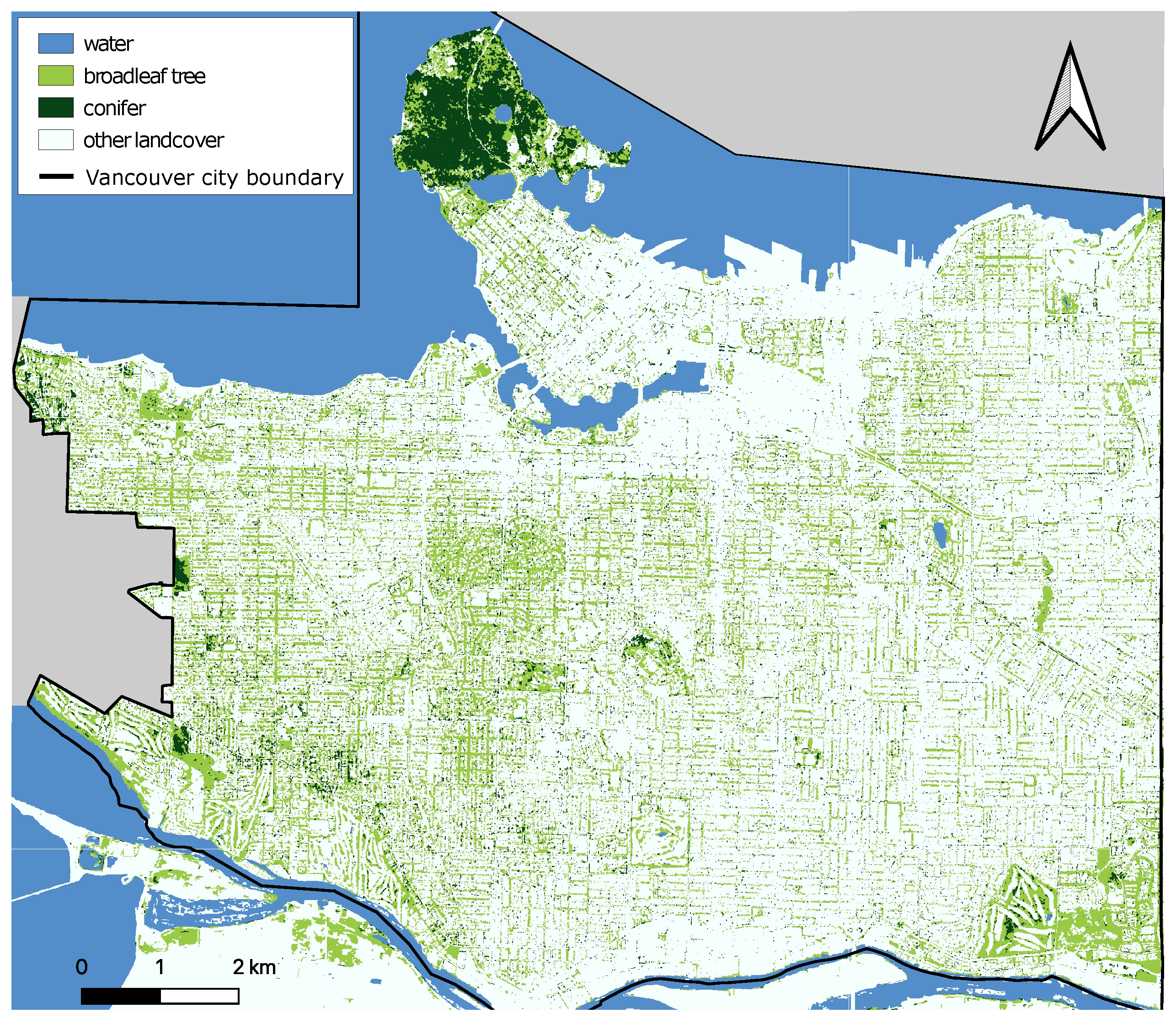
Figure 1. Map of the city of Vancouver in extreme southwestern British Columbia, Canada, showing 2019 forest cover of conifers and broadleaf trees. Note that most trees within the urban matrix are broadleaf trees. Land cover data from Metro Vancouver [30].
Atmosphere 14 00552 g001
Figure 2. Model structure showing heat fluxes among city, trees, rural air, and ground.
Atmosphere 14 00552 g002
Figure 3. Temperatures of the built environment ( T b u i l t , solid lines) and urban forests ( T t r e e , dashed lines) in the conifer (blue) and broadleaf tree (red) models when (a) 17% of the city is covered by trees, (b) 22% of the city is covered by trees, and (c) 30% of the city is covered by trees. (d) shows the built environment temperature differential when forested by different tree types at 17%, 22%, and 30% tree cover.
Atmosphere 14 00552 g003
Figure 4. Heat fluxes into and out of the built environment when 17% forested by (a) conifers or (b) broadleaf trees. (c) shows the differences between these fluxes by forest type.
Atmosphere 14 00552 g004
Figure 5. Heat fluxes into and out out of the urban forest of (a) conifer or (b) broadleaf trees. (c) shows the differences between these fluxes by forest type. Urban forest covers 17% of city.
Atmosphere 14 00552 g005
Figure 6. Evapotranspiration heat flux for conifers and broadleaf urban forests, where urban forest covers 17% of the city.
Atmosphere 14 00552 g006
Figure 7. Sensitivity analysis results showing built environment temperatures (solid lines) and tree temperatures (dashed lines) when (a) the conifer leaf area index (LAI) is set equal to that of broadleaf trees ( L A I (conifer)   =   L A I (broadleaf)), (b) conifer leaf boundary layer resistances are set equal to those of broadleaf leaves ( r a i r . a d a x i a l ( conifer ) = r a i r . a d a x i a l ( broadleaf ) and r a i r . a b a x i a l ( conifer ) = r a i r . a b a x i a l ( broadleaf ) ), (c) conifer dry leaf mass per unit leaf area was set equal to that of broadleaf trees ( m a ( conifer ) = m a ( broadleaf ) ), and (d) when conifer values for all three variables (leaf area index, boundary layer resistance, dry leaf mass) were set equal to the broadleaf values. All plots are for 17% tree cover.
Atmosphere 14 00552 g007
Table 1. Parameter values used in the model.
ParameterValueUnitSource
T b u i l t init. = 22°C
C v 3 × 10 6 J/m 3 /K[38]
s3600s/hNumber of seconds in 1 h
H0.3mOptimized to obtain reasonable city temperatures
g17, 22, or 30dimensionless [29]
α b 0.114dimensionlessAverage albedo in Vancouver, BC based on albedo values from [20] and percentage landcover values from the Land Cover Classification 2014—5 m Hybrid (updated in November 2019) dataset from http://www.metrovancouver.org/data (accessed on 26 January 2021) for all landcover classes except deciduous and coniferous trees, water, shadow, clouds, and ice
t s 5.75hTime of sunrise on August 1 in Vancouver, BC, Canada
L 49.2827 2 π 360 RadiansLatitude of Vancouver, BC
D213dayDay of year for 1 August 2020
ϵ b 0.9dimensionless[38]
σ 5.67 × 10 8 W/m 2 /K 4
v4.54m/sAverage of hourly wind velocities recorded at Vancouver Airport on 1 August 2020, via https://weatherspark.com/h/d/476/2020/8/1/Historical-Weather-on-Saturday-August-1-2020-in-Vancouver-Canada#Figures-WindSpeed (accessed on 18 January 2023)
T a i r . l o w 12.2°CHistorical August 1 low in rural Bowen Island, BC. Data from https://www.accuweather.com/en/ca/bowen-island/v0n/july-weather/53179 (accessed on 18 January 2023)
T a i r . h i g h 20.5°CHistorical August 1 high in rural Bowen Island, BC. Data from https://www.accuweather.com/en/ca/bowen-island/v0n/july-weather/53179 (accessed on 18 January 2023)
k g 1.65W/m/KFollowing [25]
T g 8°CFollowing [25]
d2mFollowing [25]
T t r e e init. = 22°C
m a (conifer)0.263kg/m 2 [39,40]
m a (broadleaf)0.073kg/m 2 [39,40]
f w 0.7dimensionless[39,41]
c w a t e r 4188J/kg/K
c d r y 1396J/kg/K[39]
H r 72.7Average humidity on 1 August 2020 in Vancouver, BC
ϵ c 0.046dimensionless[42]
K (conifer)0.52dimensionless[43]
K (broadleaf)0.7dimensionless[25]
ϵ g 0.98dimensionless[44]
α g (conifer)0.08dimensionless[20]
α g (broadleaf)0.12dimensionless[20]
h v 2450J/kg
M w 0.018kg/mol
L A I (conifer)8.6dimensionlessLAI for Pseudotsuga menziesii [45]
L A I (broadleaf)4.9dimensionlessLAI for an oak–hickory forest [46]
r c u t i c u l a r . a b a x i a l (conifer)30,303s/mFor Pseudotsuga menziesii [36,47]
r c u t i c u l a r . a b a x i a l (broadleaf)8500s/mFor Acer platenoides [36,48]
r i n t r a c e l l u l a r . a b a x i a l 17.5s/mAverage for typical plant [36,49]
r s t o m a t a l . a b a x i a l (conifer)140s/mFor Abies lasiocarpa [36,50]
r c u t i c u l a r . a d a x i a l (conifer)30,303s/mFor Pseudotsuga menziesii [36,47]
r c u t i c u l a r . a d a x i a l (broadleaf)8500s/mFor Acer platenoides [36,48]
r i n t r a c e l l u l a r . a d a x i a l 17.5s/mAverage for typical leaf [36,49]
r s t o m a t a l . a d a x i a l (conifer)1 × 10 6 s/mPseudotsuga menziesii lacks stomata on the adaxial surface [51]
r s t o m a t a l . a d a x i a l (broadleaf)1 × 10 6 s/mMost broadleaf trees lack stomata on the adaxial surface [39]
c p 29.2J/mol/K[39]
Disclaimer/Publisher’s Note: The statements, opinions and data contained in all publications are solely those of the individual author(s) and contributor(s) and not of MDPI and/or the editor(s). MDPI and/or the editor(s) disclaim responsibility for any injury to people or property resulting from any ideas, methods, instructions or products referred to in the content.