Article

Responses of Runoff and Its Extremes to Climate Change in the Upper Catchment of the Heihe River Basin, China

1
State Key Laboratory of Hydrology-Water Resources and Hydraulic Engineering, Nanjing Hydraulic Research Institute, Nanjing 210029, China
2
Key Laboratory of Groundwater Conservation of MWR, School of Water Resources and Environment, China University of Geosciences (Beijing), Beijing 100083, China
3
Southwest Jiaotong University Hope College, Chengdu 610400, China
4
College of Water Sciences, Beijing Normal University, Beijing 100875, China
*
Author to whom correspondence should be addressed.
Atmosphere 2023, 14(3), 539; https://doi.org/10.3390/atmos14030539
Submission received: 6 February 2023 / Revised: 23 February 2023 / Accepted: 26 February 2023 / Published: 11 March 2023

Abstract

:
Understanding the impact of climate change on runoff and its extremes is of great significance for water resource assessment and adaptation strategies, especially in water-scarce regions. This study aims to analyze the impact of future climate change on runoff and its extremes in the upper reaches of the Heihe River basin in northwest China. The projected runoff was derived using the Soil Water Assessment Tool with climate data from the CSIRO-MK-3-6-0 model under the scenario of RCP4.5, and a frequency analysis of runoff was performed by generalized extreme value distribution. The results indicate that, compared with the baseline period of 1961 to 2000, the minimum and maximum temperatures in the period 2031 to 2070 were predicted to increase by 2.5 °C on average. The precipitation in most months was also predicted to increase, with an average rise of 16.5%. The multi-year average runoff was projected to increase by 8%. The annual mean and extreme flows were also expected to rise under future climate change at different return periods, and the low flow was expected to increase the most.

1. Introduction

The Heihe River basin (HRB) is the second largest inland river basin in northwest China. Water scarcity is one of the critical problems that the basin has to face. Under warming climate conditions, the total runoff over the upper stream has been observed to increase over the past 60 years (1958–2014) [1]. It increased by 30.5% during the period from 1964 to 2013 [2] and by 6.1 mm per decade during the period from 1980 to 2010 [3]. Meanwhile, the levels of extreme runoff have also changed. For example, flood events in the upper catchment have increased, while low-water events have decreased [4,5]. Specifically, from 1960 to 2014, Cheng et al. (2020) found that extreme floods in the upstream areas showed an increasing trend, whereas the extremely low water showed a decreasing trend [4]. Such changes in runoff extremes necessitate changes in local water resources management, flood control, and disaster reduction strategies.
Under future climate change conditions, whether the risk of water resource shortages changes, continues, or declines is still a matter of great concern. We summarized some related studies focusing on runoff responses to future climate change. For example, Wu et al. (2015) concluded that the water yield would increase by 9.8% as a result of climate change during the period 2006–2030 [6]. Zhang et al. (2016) reported that 11.4% and 12.5% increases in runoff are projected to occur under scenarios RCP4.5 and RCP8.5, respectively, in the near future [7]. Li et al. (2020) found that the projected precipitation during 2021–2050 and 2051–2080 would produce a 5.6% and 6.7% increase in runoff, respectively [8]. In spite of the great increase in attention given to future runoff, the responses of runoff extremes to future climate change are rarely addressed. Thus, the aim of this study is to focus on how the total and extreme runoff varies and how the frequency of such events is expected to change in the future under climate change in the upper catchment of the HRB, which will provide insights for decision-makers attempting to mitigate the corresponding impacts.
One common way to study the impact of climate change on runoff is by using general circulation models (GCM) combined with hydrological models. As far as we know, as many as nearly 30 GCMs have been tested in this basin. Li et al. (2020) and Wang et al. (2020) reported that in simulating the observed precipitation and temperature data from 1960 to 2005, the top three models for this basin are CSIRO-Mk3.6.0, CCSM4, and CanESM2, respectively [8,9]. In the references of Yan et al. (2018) and Wang et al. (2019), a slightly different ranking was found, with CNRM-CM5, MPI-ESM-LR, and MPI-ESM-MR being the top three [10,11]. However, these models only evaluated their performance in terms of precipitation without considering temperature, which is another important GCM output and is always used as a hydrological modeling input [10,11]. Consequently, the CSIRO-Mk3.6.0 model, ranked first by Li et al. (2020) and Wang et al. (2020) [8,9], is selected here to derive the future climate scenario over the upper reach of the basin. As for hydrological modeling tools, some typical models have been used in this basin, including SWAT [1,2,3,5,6,7,12,13,14,15,16,17,18,19,20,21,22,23,24,25,26,27,28], WASMOD [28], PRMS [29], VIC [30], SRM [31], and GBEHM [32,33,34]. Among them, the most widely used is the SWAT model, which is used in more than 75% [23] of the studies we identified, owing to its advantages of being open source, highly developed, more flexible, etc., and this model has been widely applied in various basins worldwide.
The annual maximum series (AM) and the peaks over a threshold (POT) series are two common measures of extreme events [35]. The POT series is regarded as more advantageous than the AM series, especially in cases when only a short period of records is available, as it provides more information about the extremes involved [36]. However, the fact that the peaks over a certain threshold value in the POT series might not form an independent time series can restrict its application in some cases. Li et al. (2016) stated that the estimated return levels from the AM and POT series were quite comparable [37]. Rao and Hamed (1999) found that when λ is small (e.g., λ < 1.65, λ is the mean number of peaks per year included in the POT series), the AM series is statistically more efficient [38].
Frequency analysis is a critical aspect of water resources management and hydrological design. As for the choice of a probability distribution for a given application, several researchers have investigated the suitability of different probability distributions in different applications [39,40,41,42]. However, most results show that the optimal probability distribution varies across different regions. For example, the generalized normal distribution (GNO) resulted in the best fit to flood flows in northern Tunisia, whereas the GNO and generalized extreme value (GEV) distributions gave the best fit in central/southern Tunisia [40]. Log perason III (LP3) and GEV performed similarly in estimating the return levels of floods in southeast Australia [39] and ranked as the top two distributions in flood fitting in Khwazakhela [42]. More recently, there has been an increased focus on the use of GEV distributions worldwide. Gubareva et al. (2011) also compared different distributions in fitting floods in rivers in Austria, Siberia, and the Far East and found that GEV showed a clear predominance over others, such as Pearson III and Lognormal distributions, in all regions with various climate conditions [41]. Based on these observations, GEV is selected to fit the runoff series in this study.
The outline of the paper is as follows. The study area and data are described in Section 2, and the methods used are described in Section 3. The future climate scenarios and their corrections, the construction, evaluation, and prediction of the SWAT model, as well as frequency analysis of future runoff, both in total and in extremes, are discussed in Section 4, followed by the conclusions in Section 5.

2. Study Area and Data Description

The HRB has an arid continental climate. According to its terrain, the basin is divided into the upper, middle, and lower reaches. The upper reach extends from Qilian Mountain to the Yingluoxia gorge (E98°34′-101°09′ and N 37°43′-39°06′) (Figure 1); it is the main recharge area of the basin. The upper reach has an altitude of 2000-5500 m, an annual average temperature of less than 2 °C, and an annual precipitation of 200–500 mm. The middle and lower reaches contain few oases. The largest one is Zhangye oasis, located in the middle reach, an important agricultural area in Gansu province. This area produces 35% of the commercial grain of the province on 5% of the cultivated land (http://www.zhangye.gov.cn/zjzy/lswh/202212/t20221204_950374.html (accessed on 2 December 2022)). The number and areas of oases in the basin largely depend on the amount of water from the upper reach. The availability of water resources in the basin is limited, and the water resource system is fragile.
The data required for establishing the SWAT model include a digital elevation model (DEM), and land use, soil, meteorological, and runoff data. Details on the data are listed in Table 1. Meteorological and hydrological data include historical daily precipitation, minimum and maximum temperatures, wind speed, sunshine hours, relative humidity, and runoff from 1960 to 2014. The precipitation data are gridded data with a 3 km resolution. Other meteorological data and runoff data were obtained from gauge observations. The missing runoff data for 1988 and 1989 were interpolated by calculating the multi-year average. Table 2 provides the location of the stations.
The prediction period was 2031 to 2070, and the predicted data were compared with the data from the 1961 to 2000 baseline period. The meteorological data from 2031 to 2070 were obtained from the CSIRO-MK-3.6.0 model released by CMIP5 under the RCP4.5 scenario. The time scale was daily, and the resolution was 1.875° × 1.875°.

3. Methods

3.1. Downscaling and Bias Correction of Future Climate Data

Since the horizontal grid distance of a GCM is usually hundreds of kilometers, it is necessary to downscale the GCM to reduce the error. This study performed linear interpolation using the interp3 function in MATLAB to resample the spatial resolution of the CSIRO-Mk-3-6-0 model from 1.875° × 1.875° to 0.25° × 0.25°.
The original GCM output data have been bias-corrected using the delta change approach; this approach is typically used in related studies [43,44]. Here, the precipitation data derived from the GCM in the future period (2031–2070) and the baseline period (1961–2000) were compared, and the percentage change was calculated. The result was multiplied by the annual mean precipitation in the baseline period to obtain the change in annual mean precipitation in the future. In contrast, we used the absolute change for temperature. Detailed descriptions of the delta change approach can be found in Zhao and Xu (2007) [45].

3.2. SWAT Model

The SWAT model is a distributed watershed hydrological model. It uses geographic data to divide basins into sub-basins, and each sub-basin contains one or more hydrological response units (HRUs). The model can simulate surface runoff using the soil conservation service (SCS) curve or the Green and Ampt method. It uses degree days to estimate snow accumulation and melting. SWAT-CUP is a program developed specifically for SWAT model parameter calibration. It uses the Glue, Parasol, Sufi2, MCMC, and PSO methods. We used SUFI2 for parameter sensitivity analysis and calibration. This method has a short optimization time and is suitable for basins with relatively simple runoff changes. The SUFI2 algorithm randomly generates a set of parameters through Latin-Hypercube simulations and inputs them into the SWAT model to calculate the objective function.
Within the framework of AVSWAT 2015, the study area was divided into 11 sub-basins and 113 HRUs based on the soil type, land use, and topography. The SCS curve method, Muskingum, and Penman–Monteith methods were used for surface runoff volume estimation, flow routing, and potential evapotranspiration estimation, respectively. SWAT-CUP was used for parameter sensitivity analysis, model calibration, and validation. Runoff data from the Yingluoxia station from 1985 to 1989 were chosen as the warm-up period, data from 1990 to 2005 were used for model calibration, and the last 9 years (2006–2014) were used for validation.
The determination coefficient ( R 2 ) and the Nash–Sutcliffe efficiency coefficient ( N S E ) were used to evaluate model performance. The equations are as follows:
N S E = 1 t = 1 T Q o t Q m t 2 t = 1 T Q o t Q O
R 2 = t = 1 T Q o t Q O Q m t Q m ¯ t = 1 T Q o t Q o ¯ 2 t = 1 T Q m t Q m ¯ 2
where Q o t and Q m t are the observed and simulated values at time t, and T is the total time. The R 2 value range is [0, 1]. The larger the value of R 2 , the better the simulation result of the model. The range of the NSE values is [−∞, 1]. The larger the value of NSE, the higher the model reliability. An NSE value between 0 and 1 is generally considered an acceptable performance level, and a value much smaller than 0 indicates poor model performance [46]. The closer the N S E and R 2 values are to 1, the better the model performance. The model performance ratings are listed in Table 3.

3.3. Frequency Analysis

Since hydrological periodicity exists, and the λ value is small (it is estimated at 1.2 in this study), the AM series was selected to detect extreme events. The annual, monthly maximum and minimum series were chosen and denoted as the high-flow and low-flow series, respectively. This strategy ensured the full use of limited data and the independence of the series.
The GEV distribution was selected to fit the mean and the high- and low-flow series in this study because it is widely used. Equation (3) defines the probability density function (PDF) for this distribution.
F x = e x p 1 k x β α 1 k , k 0 e x p e x p x β α , k = 0
where k , α , and β are the shape, scale, and position parameters, respectively.
The theoretical return period of the runoff was obtained by calculating the quantile; it was compared with the empirical return period. The quantile equation is:
X T = β + α k 1 l n 1 1 λ T k , k 0 β α l n l n 1 1 λ T , k = 0
where λ is the average crossover rate for many years and λ = n / N , where n is the sample size and N is the total length of data. For the AM sequence, λ = 1 .
The Kolmogorov–Smirnov (K-S) test and the Anderson–Darling (A-D) test were used to test the goodness of fit of the GEV. The A-D test is an improvement of the K-S test; it gives more weight to the tail of the distribution. The test rejects the assumption of a GEV distribution if the test statistic is greater than the threshold at a given significance level.

4. Results

4.1. Future Climate Change

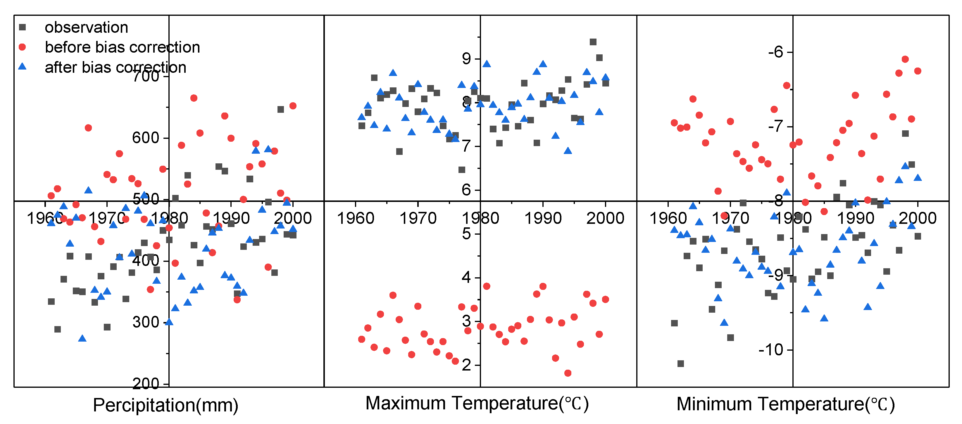
The meteorological data derived from the CSIRO-Mk3.6.0 model are compared with the corresponding observations from 1961 to 2000 to ensure the accuracy of the meteorological data predicted by the GCM. The results are shown in Figure 2 and Figure 3.
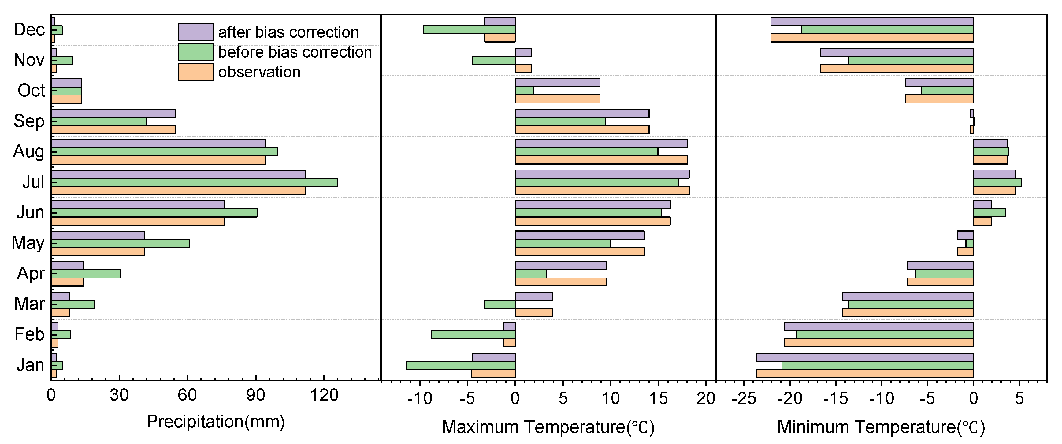
Many precipitation values are overestimated (Figure 2). The interannual distribution shows that the values are overestimated in ten out of twelve months (except for September and October), and only the data for September are underestimated (Figure 3). At the seasonal scale, the multi-year average spring precipitation is 110.31 mm, which is overestimated by nearly 73%, and the multi-year average summer precipitation is 316.07 mm, which is overestimated by 12%. The maximum temperature is underestimated (about 5 °C on average), and the minimum temperature is overestimated (about 1.5 °C on average) (Figure 2). At the inter-annual scale, only the maximum temperature in June and July exhibits a good fit with the observations, whereas the data in the other months are substantially underestimated. The minimum temperature shows a good fit with the observations only in July and August, whereas the data are overestimated in the other months.
As shown in Figure 2 and Figure 3, the bias-corrected data are much closer to the observations than the uncorrected data. The multi-year average relative errors of the maximum and minimum temperatures decrease substantially from 64% and 16% to less than 1% after bias correction. The bias-corrected precipitation data are also more consistent with the observations than the uncorrected data. The multi-year average relative error decreases from 23% to 3%, indicating the advantage of bias correction.
The performance of the bias-corrected GCM in reproducing the extreme precipitation at monthly scales (maximum monthly precipitation) is shown in Figure 4. Figure 4a indicates that the extreme precipitation data derived from the GCM is generally consistent with the observations, whereas the values are overestimated in some years (e.g., 1967, 1975, and 1985). The multi-year average value (denoted by “□” in the box plot) is overestimated by 13% (Figure 4b). After bias correction, the data are more consistent with the observations, and the errors of the mean, median, and 75% quantile decrease from 13%, 18%, and 10% to 0.5%, 1.7%, and 5.3%. This result demonstrates that the performance of the bias-corrected GCM in reproducing the extreme monthly precipitation was satisfactory.
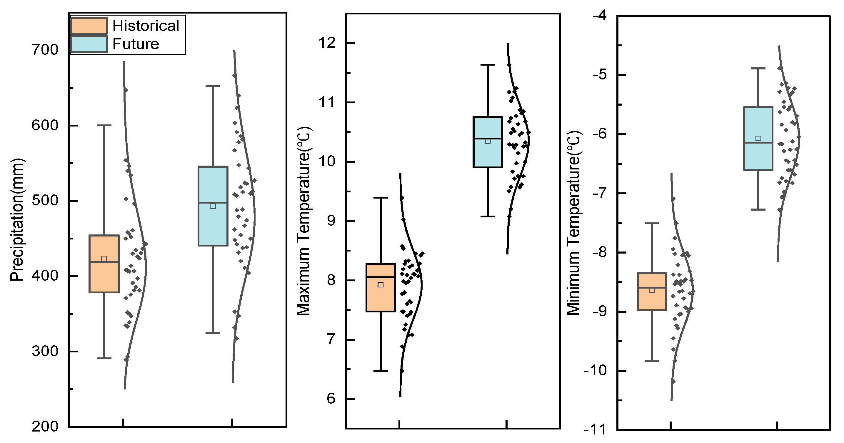
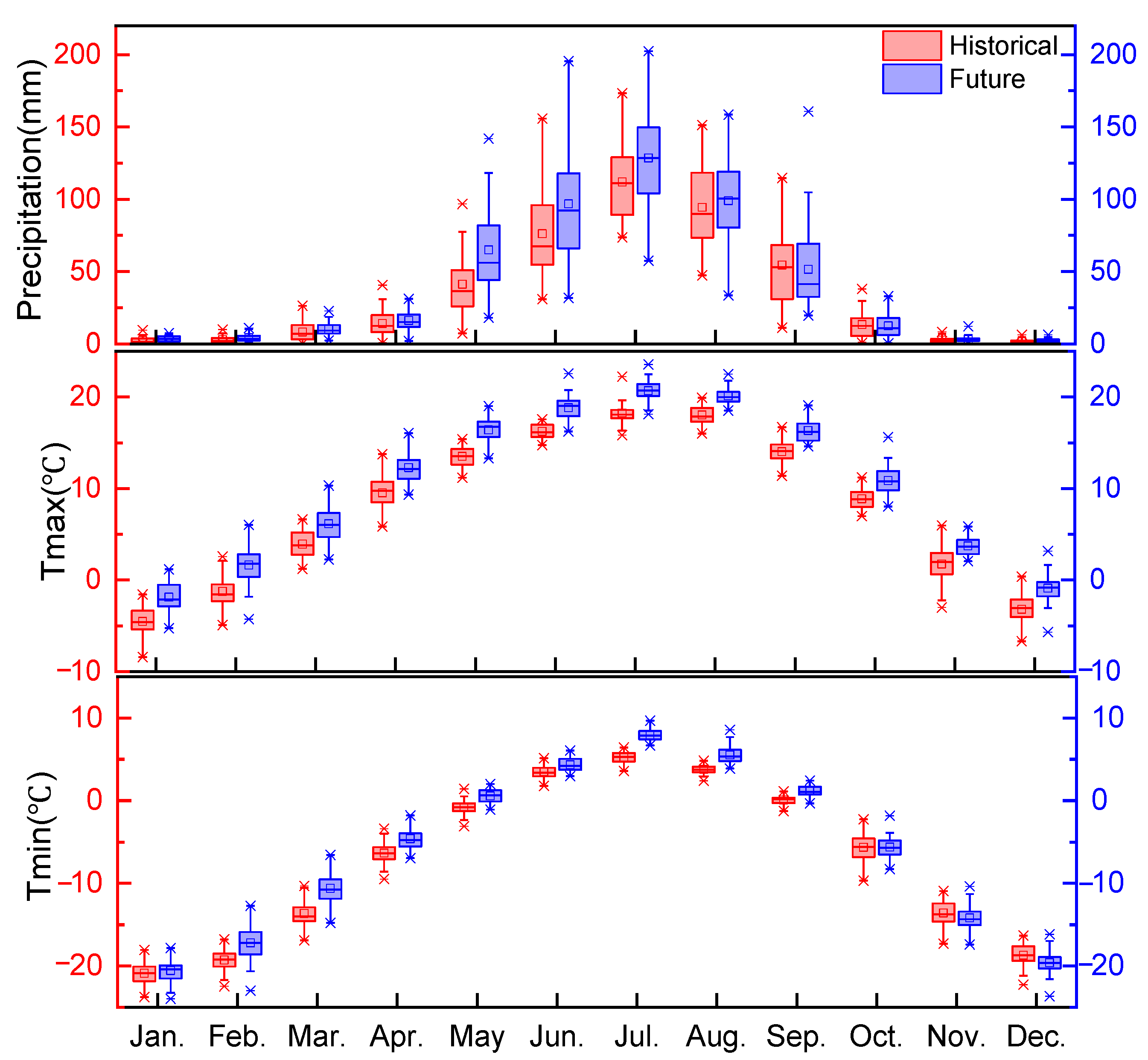
The historical and future temperature and precipitation values derived from the CSIRO-Mk3-6-0 model after bias correction are presented in the box plot in Figure 5, showing the mean, median, upper and lower quartiles, upper and lower limits, and point fitting results. The mean, maximum, and minimum temperatures and the upper and lower quartiles and limits are higher in the future than historically (1961–2000). The maximum and minimum temperatures are projected to increase by 2.4 °C and 2.6 °C, respectively, on average. At the inter-annual scale, both temperatures are projected to rise in nearly all months (Figure 6). The minimum temperature in March exhibits the largest increase (about 3.0 °C), followed by February, April, May, July, and August, with increases of more than 1.0 °C. The maximum temperature of each month is projected to rise steadily, with increases of more than 2 °C in ten out of twelve months and less than 2 °C in October and November. These results indicate that the temperature rise will continue in the coming decades, consistent with global climate warming.
The future precipitation is also projected to increase compared to 1961 to 2000, with an average increase of 16.5%. At the inter-annual scale, the largest increases occur in May, January, and December (more than 50%), and decreases are observed only in September and October (about 5%).
In summary, the future climate in the basin will likely be warmer and wetter than in the historical baseline period, increasing the probability of extreme hydrological events in the future.

4.2. SWAT Model Performance

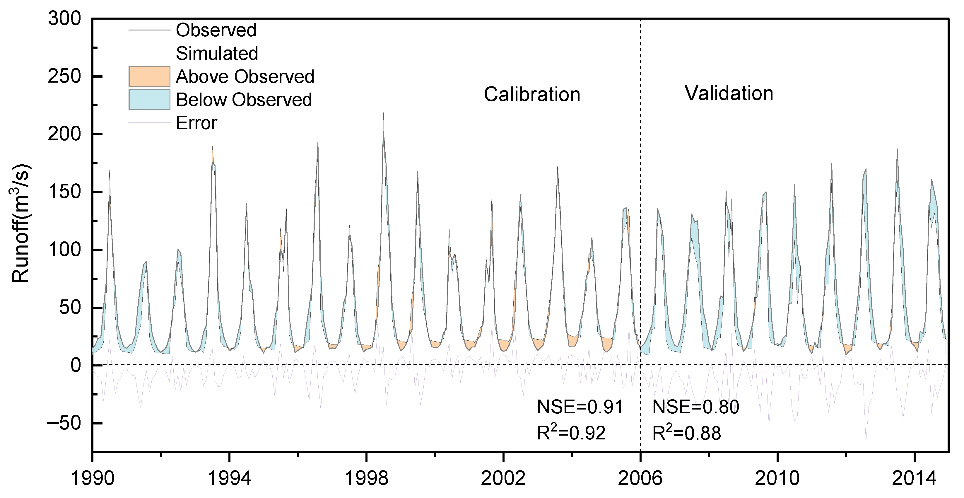
Figure 7 shows the hydrographs at the Yingluoxia station derived from AVSWAT2015 and SWAT-CUP, together with the errors of the simulated runoff. There is good consistency between the calibration and validation periods. The major patterns of the hydrograph are simulated accurately. The evaluation indicators are displayed in Figure 7. The NSE and R2 are greater than 0.80 in both periods. As shown in Table 3, the SWAT model shows a very good performance in simulating the runoff series in the study area. In contrast to other studies [5,6,7,12,13,14,15,16,17,18,19,20,21,22,23,24,25,26,27,28], a moderate performance is obtained in this study.
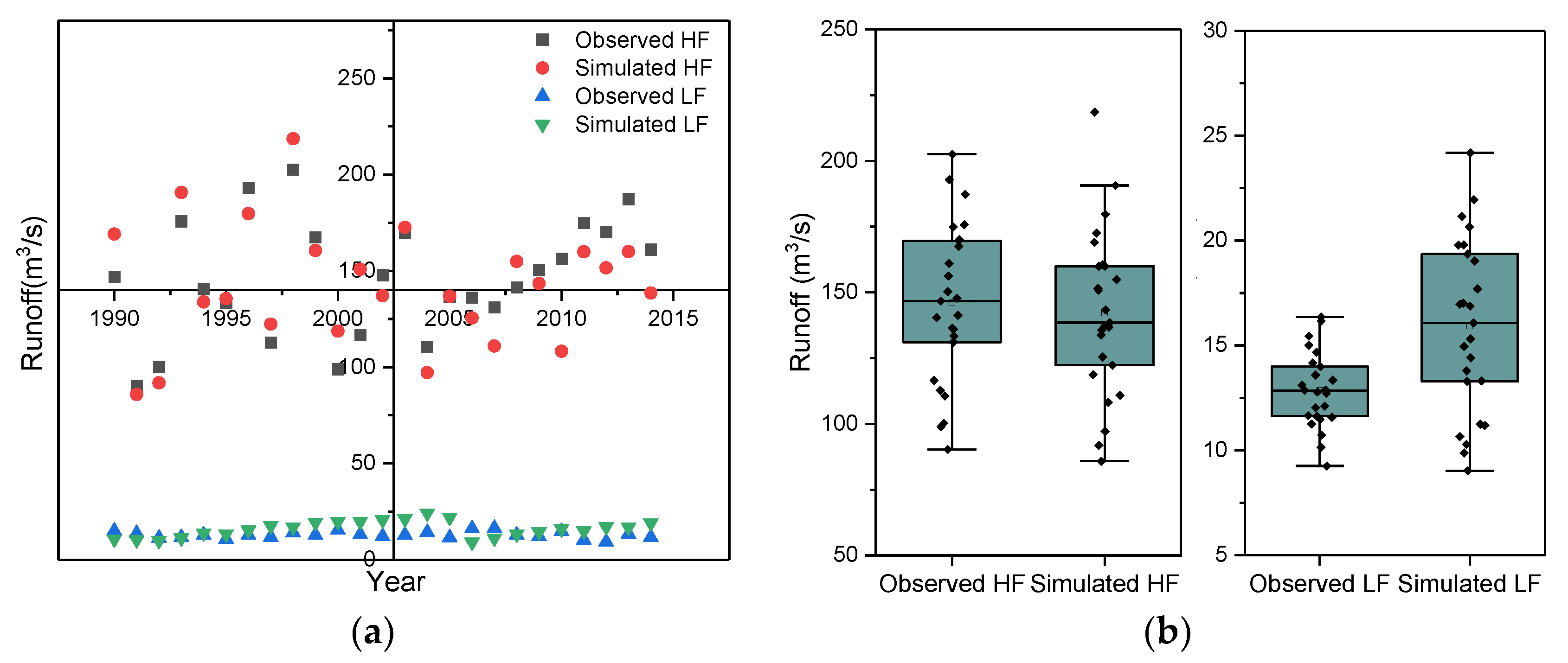
We extracted the high-flow and low-flow series (Figure 8). The relative errors range from −31% to 29% for the high flows and from −44% to 91% for the low flows. The performance of simulating the high flows and low flows is satisfactory. Figure 8b indicates that the mean, median, and 25% and 75% quantiles of the high flows were underestimated by 3%, 6%, 3%, and 6%, respectively; however, the percentages are acceptable. The simulation performance is inferior for the low flows; the mean, median, and 25% and 75% quantiles were overestimated by 24%, 25%, 6%, and 39%, respectively. The model performance is higher for high flows than for low flows.

4.3. Projected Runoff and Extremes

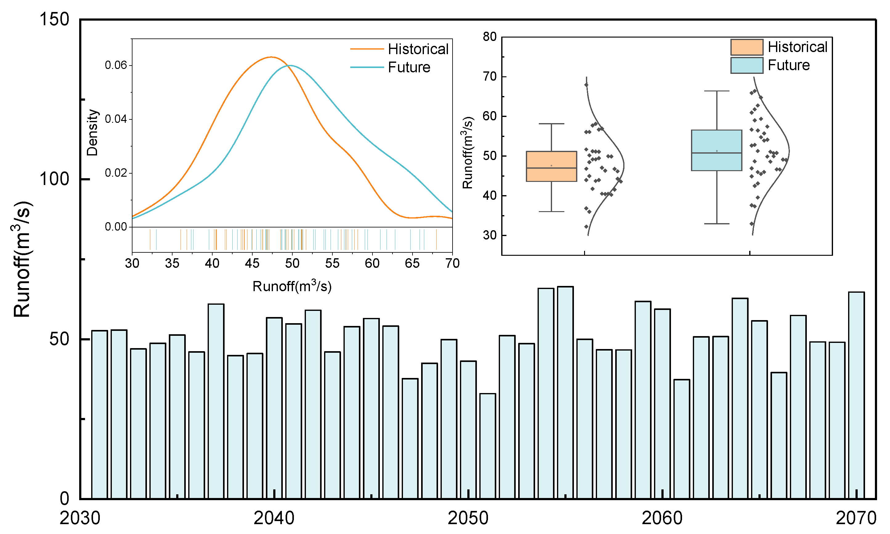
The future runoff predicted by the validated SWAT model with the corrected input data of future precipitation and temperature is shown in Figure 9. The annual mean runoff from 2031 to 2070 is projected at 51 m3/s, which is 8% higher than in the baseline period. The 25% and 75% quantiles are also projected to increase.
Figure 10 shows the inter-annual variability of the projected runoff. Similar to the baseline period, the largest projected runoff will occur in summer (49%), followed by autumn (20%), spring (18%), and winter (13%). The projected runoff differs in different seasons and months and is expected to increase or decrease compared to the baseline period. It is projected to increase the most in winter (88.5%), followed by spring (30.8%). However, the runoff is predicted to decrease in some months in summer and autumn (September, October, July, and August). The greatest decrease is projected to occur in September (18%), which may be caused by the lower precipitation in this month, as shown in Figure 6.
The projected runoff extremes are also considered since they are more sensitive to climate change at the regional scale. Figure 11 and Table 4 show the statistical results of the projected high- and low-flow series. The mean value of the high-flow series is projected to decrease slightly by 3%, the maximum value (229.3 m3/s) is predicted to increase by 13%, and the minimum value (67.15 m3/s) is predicted to decrease by 15%. The coefficient of variation is projected to increase by 27%, indicating an increase in the degree of variation of the high flows. The data suggest an increased flood risk during the wet season, resulting in challenges in water resource allocation and management.
The mean and extreme values of the low flows are projected to increase substantially compared to the baseline period, with percentages of 97%, 65%, and 120% for the mean, maximum, and minimum values, respectively. The degree of variation tends to decrease according to the coefficients of variation and standard deviation. This finding indicates a higher availability of water resources in the dry season, reducing the potential of water scarcity in the dry season in the future.

4.4. Results of Frequency Analysis of Projected Runoff and Extremes

The K-S test and A-D tests were used to evaluate the GEV distribution. The critical values are 0.19 and 2.50 for the two tests, respectively, at the 0.05 significance level. If the statistic value is lower than the critical value, the data set has a GEV distribution; otherwise, it does not. Table 5 shows that all the statistic values are lower than the critical values, indicating that the data series has a GEV distribution. The optimal parameter values of the series are presented in the table.
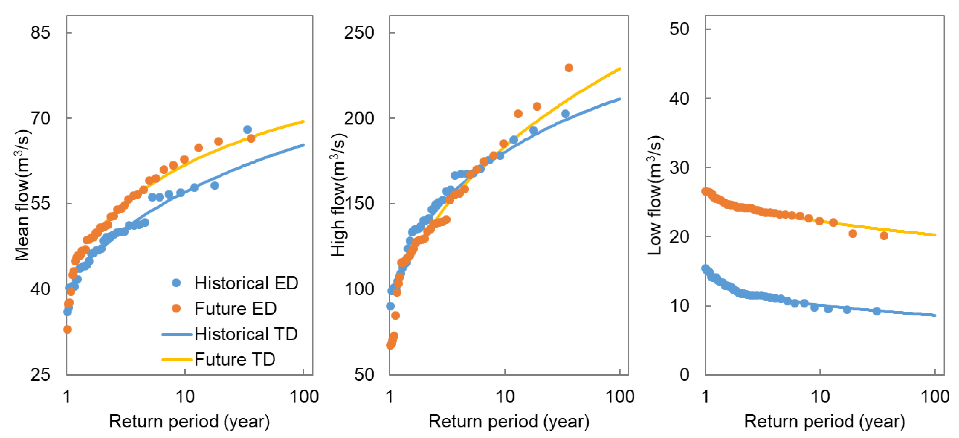
Figure 12 shows the estimated return levels of the annual mean flow and the extremes. The solid lines are for data with the theoretical GEV distribution, and the dots are from data with the empirical distribution, which is calculated from P = i 0.44 n + 0.12 , where i indicates the order, and n indicates the length of data (i = 1, 2, …, n). The blue and yellow lines represent the historical data and future estimations. It is notable that the annual mean flow is expected to increase in the future at different return periods, e.g., 8.7% increases for a 5-year return level, 8.4% increases for a 10-year return level, and 7.8% increases for a 20-year return level (Figure 13). These results suggest that water shortages will be alleviated in the future.
Compared to the baseline period, the return levels of the high flows are expected to increase over a 10-year return period, with 3.9%, 5.1%, 6.6%, and 8.4% increases in the 20-year, 30-year, 50-year, and 100-year return periods (Figure 13), respectively, suggesting that the high flows will be more extreme, i.e., for a given return level of high flows, the return period will become shorter. For instance, the return period for a 200 m3/s high flow was 37 years during the historical period and will be 21 years in the future. These results indicate that this area will experience more flooding in the future, resulting in increased challenges related to local flood control.
In addition, much more low flows are expected in the future. For instance, the low flow for the 20-year return period is 9.56 m3/s in the baseline period; it increases to 21.54 m3/s in the future, a more than two-fold increase. The low flow for the 100-year return period is expected to exceed 20 m3/s, much larger than the maximum low flow in the baseline period. An increase in the low flow means that spring droughts will be alleviated, which benefits agriculture in the middle reach and natural ecosystems in the lower reach.

4.5. Discussion

The total and extreme runoffs under future climate change were projected, and the frequency variations of these events were obtained. The future total runoff is expected to increase by 8% compared with the baseline period. This result is comparable with the findings of previous studies. For example, Wu et al. (2015) predicted a 9.8% increase in runoff during 2006–2030 compared to 1981–2005 due to climate change [6]. Zhang et al. (2016) observed an 11.4% increase in runoff from 2021 to 2050 compared to 1981–2010 [7]. Li et al. (2020) estimated a 5.6–6.7% increase in runoff due to increased precipitation [8]. However, it should be emphasized that not all studies predicted increased runoff in the future. Some predicted a decrease in the runoff. For instance, Wang et al. (2018) predicted a decrease in the runoff by approximately 5 mm/10 a by 2060 when considering the effects of global warming [47]. Zhang et al. (2015) projected that the runoff would decline regardless of which cases were considered, i.e., only the effects of climate change or the combined impacts of climate change and LUCC [23]. Wu et al. (2015) estimated that the land-use change would result in a 1.8% decrease in the runoff, whereas climate change would cause a runoff increase of 9.8% from 2006–2030 [6]. The inconsistencies of these results are related to many factors, such as the simplification of complex hydrological processes, the diversity of hydrological models, and the difference in the time span of historical and future scenarios.
Our study predicts that the annual mean and the high and low flows will increase in the future. The increases in the annual mean runoff and the high flows can be attributed to increased precipitation. As shown in Figure 5 and Figure 6, an average precipitation increase of 16.5% is predicted in the future compared to the baseline period, and 27%, 15%, and 5% increases will occur in June, July, and August, respectively; these are the periods with the highest probabilities of high flows. An increase in precipitation would cause runoff increases. In addition, temperature increases would also contribute to an increased runoff because more water would be released from glaciers, snow, and permafrost. It was estimated that 25% of the annual average runoff was attributed to snowmelt, and 4% resulted from glacier melt [48]. Wu et al. (2015) found that glacial melt increased runoff by about 2.3 mm, contributing 8.9% to runoff in 2010 [24].
Increased temperatures in the future would have a more significant effect on low flows, which generally occur in spring or winter, than on high flows. Wang et al. (2006) concluded that about 75% of the spring runoff was attributed to snowmelt and glacier melt [49]. Zhang et al. (2016) predicted that the mean snowmelt amount would increase by 4.3–5.8% if the mean temperature increased by 1.2–2.1 °C [7]. In this study, the minimum and maximum temperatures in spring are projected to rise by 2.8 °C and 2.6 °C, on average, in the future. If this occurred, glaciers, snow cover, and permafrost in the study area would contribute more to river runoff in the dry season. Although some studies have reported that approximately 90% of the glaciers in the HRB are expected to disappear by the 2040s or 2060s, glacier runoff will increase before this period and decrease after [47,48]. Therefore, the contributions of glacier melting to runoff in the dry season under warming scenarios cannot be ignored, especially in the near future. Although the projected increase in low flows in the future can be explained by increases in glaciers and snow melting due to increased temperatures, it should be noted that overestimations of historical low flows will result in overestimations of future low flows. As shown in Figure 7 and Figure 8, the baseflow simulation result was not as good as that of other flows; it was overestimated during the baseline period, which may lead to overestimations of the baseflow in the future.
Given the significant changes in future runoffs and extremes, the water resource availability and seasonality in the study area would vary. Thus, water use in the middle and lower reaches should be adjusted to adapt to these changes. This study can help local water resource managers and decision-makers develop adaptive strategies for effective water resource and ecological management under a changing climate.
In addition to climate change, human activities (e.g., land use/land cover change, the construction of water conservancy projects, and human water use) are major factors affecting runoff changes. The reasons for not considering the impacts of human activities in this study are as follows. First, many studies have shown that climate change impacts on runoff in our study area were more significant than other factors [2,3,19,20,23], and the contribution of climate change to runoff increased over time [5] and by 87% from 2004 to 2014 [1]. Second, more than 96% of the study area is covered by forest, grassland, and unused land, and only less than 0.5% is covered by buildings and cropland [8]. Human activities are limited in the study area due to the high altitude (1674 to 5108 m) and small population (less than 1.5 million). Furthermore, there are many glaciers and areas with snow cover, permafrost, and alpine meadows, with patches of shrubs and forests above 3600 m. These areas would be affected more by climate change. Thus, we focused on the effects of future climate change.
Two other issues were not considered in this study: non-stationarity and uncertainty. A time series is often assumed to be stationary in frequency analysis. Although non-stationary runoff caused by climate change or human activities has been reported in the literature [50], the identification of physical processes and other factors influencing non-stationarity is challenging and difficult to model, preventing reliable predictions [51]. No solid consensus has been reached on whether non-stationary hydrological frequency analysis is always superior to stationary hydrological frequency analysis [51]. Non-stationary frequency analysis is more complex and has higher uncertainty than stationary application frequency analysis due to a more complex model structure and more model parameters [52]. Therefore, we assumed that the runoff regimes were stationary in this study, resulting in model uncertainty. Additional uncertainty sources include the model type (including GCM, SWAT, GEV, and the bias correction method), model input data, and model parameters and their transferability. For example, we assumed that the parameters of the hydrological model were the same in the past and in the future, which may result in prediction uncertainties. In addition, only one GCM model was employed in this study. Although it was proven to be superior to other GCMs and applicable to the HRB [8,9], uncertainty cannot be avoided. Some researchers used the mean of multi-model ensembles (MMEs) [53] rather than choosing an optimal model. Other studies found that an MME was a potential solution to limitations of hydrological projections under a changing climate [54]. Climate signals are also highly uncertain, and using only one GCM does not adequately represent the uncertainty of future climate signals. Therefore, the uncertainty need to be investigated in subsequent studies.

5. Conclusions

This study used meteorological data from the CSIRO-M-K-3-6-0 model and the SWAT model to predict future runoff due to climate change in the upper reaches of the HRB in China. The probability distributions of future runoff and extreme values were calculated using the GEV model. The main conclusions are as follows:
(1)
The temperature and precipitation were projected to increase in the future. The minimum and maximum temperatures were predicted to increase by 2.4 °C and 2.6 °C compared with the baseline period (1961–2000). The precipitation was projected to increase by 16.5%, with the largest increases exceeding 50% in January, May, and December and decreases of 5% in September and October.
(2)
The multi-year average runoff in the basin was predicted to increase by 8%, and the highest increase would occur in winter (89%). In contrast, decreases in the average runoff were predicted in summer and autumn, with the largest decline in September (18%).
(3)
Higher annual mean runoffs with different return periods were predicted, with 6.3–7% increases in the 50–100 year return period, 7–8% increases in the 10–50 year return period, and more than 8% increases in the 10-year return period. High flows were projected to increase by 3.9%, 6.6%, and 8.4% in the 20-year, 50-year, and 100-year return periods, respectively. The low flows were predicted to increase two-fold compared to the baseline period, alleviating water shortages, especially in the dry season, but increasing the flood risk in the rainy season in the basin.

Author Contributions

Conceptualization, Z.L. (Zhanling Li) and W.L.; methodology, Z.L. (Zhanling Li) and W.L.; software, W.L.; validation, Z.L. (Zhanling Li) and W.L.; formal analysis, W.L. and Z.L. (Zhanling Li); resources, Z.L. (Zhanling Li) and Z.L. (Zhanjie Li); data curation, W.L. and X.L.; writing—original draft preparation, Z.L. (Zhanling Li) and W.L.; writing—review and editing, Z.L. (Zhanling Li), Z.L. (Zhanjie Li) and X.L.; visualization, Z.L. (Zhanling Li), Z.L. (Zhanjie Li); supervision, Z.L. (Zhanling Li); project administration, Z.L. (Zhanling Li); funding acquisition, Z.L. (Zhanling Li). All authors have read and agreed to the published version of the manuscript.

Funding

This study is supported by the Belt and Road Special Foundation of the State Key Laboratory of Hydrology-Water Resources and Hydraulic Engineering (2021nkms03).

Institutional Review Board Statement

Not applicable.

Informed Consent Statement

Not applicable.

Data Availability Statement

The GCM datasets used in this study can be downloaded from http://www.ceda.ac.uk (accessed on 3 January 2023). The runoff datasets in the study area are unavailable due to privacy.

Conflicts of Interest

The authors declare no conflict of interest.

References

  1. Shang, X.; Jiang, X.; Jia, R.; Wei, C. Land Use and Climate Change Effects on Surface Runoff Variations in the Upper Heihe River Basin. Water 2019, 11, 344. [Google Scholar] [CrossRef] [Green Version]
  2. Yin, Z.; Feng, Q.; Zou, S.; Yang, L. Assessing Variation in Water Balance Components in Mountainous Inland River Basin Experiencing Climate Change. Water 2016, 8, 472. [Google Scholar] [CrossRef] [Green Version]
  3. Yang, L.; Feng, Q.; Yin, Z.; Wen, X.; Si, J.; Li, C.; Deo, R.C. Identifying separate impacts of climate and land use/cover change on hydrological processes in upper stream of Heihe River, Northwest China. Hydrol. Process. 2017, 31, 1100–1112. [Google Scholar] [CrossRef]
  4. Cheng, W.; Xi, H.; Zhang, J. Response of runoff to extreme climate change in the upper reaches of the Heihe river. Plateau Meteorol. 2020, 39, 120–129. [Google Scholar]
  5. Luo, K.; Tao, F.; Moiwo, J.P.; Xiao, D. Attribution of hydrological change in Heihe River Basin to climate and land use change in the past three decades. Sci. Rep. 2016, 6, srep33704. [Google Scholar] [CrossRef] [PubMed] [Green Version]
  6. Wu, F.; Zhan, J.; Su, H.; Yan, H.; Ma, E. Scenario-Based Impact Assessment of Land Use/Cover and Climate Changes on Watershed Hydrology in Heihe River Basin of Northwest China. Adv. Meteorol. 2015, 2015, 1–11. [Google Scholar] [CrossRef] [Green Version]
  7. Zhang, A.; Liu, W.; Yin, Z.; Fu, G.; Zheng, C. How Will Climate Change Affect the Water Availability in the Heihe River Basin, Northwest China? J. Hydrometeorol. 2016, 17, 1517–1542. [Google Scholar] [CrossRef]
  8. Li, Z.; Li, Q.; Wang, J.; Feng, Y.; Shao, Q. Impacts of projected climate change on runoff in upper reach of Heihe River basin using climate elasticity method and GCMs. Sci. Total Environ. 2020, 716, 137072. [Google Scholar] [CrossRef]
  9. Wang, J.; Li, L. Application of entropy weighted TOPSIS method for selection of general circulation models. South North Water Transf. Water Sci. Technol. 2020, 18, 14–21. [Google Scholar]
  10. Yan, C.; Liu, L.; Huang, G. Multi-model projections of future climate change under different RCP scenarios in arid inland region of north China. J. Drain. Irrig. Mach. Eng. 2018, 36, 1193–1199. [Google Scholar]
  11. Wang, R.; Cheng, Q.; Liu, L.; Yan, C.; Huang, G. Multi-Model Projections of Climate Change in Different RCP Scenarios in an Arid Inland Region, Northwest China. Water 2019, 11, 347. [Google Scholar] [CrossRef] [Green Version]
  12. Zhang, L.; Jin, X.; He, C.; Zhang, B.; Zhang, X.; Li, J.; Zhao, C.; Tian, J.; DeMarchi, C. Comparison of SWAT and DLBRM for Hydrological Modeling of a Mountainous Watershed in Arid Northwest China. J. Hydrol. Eng. 2016, 21, 04016007. [Google Scholar] [CrossRef]
  13. Wang, J.; Huo, A.; Zhang, X.; Lu, Y. Prediction of the response of groundwater recharge to climate changes in Heihe River basin, China. Environ. Earth Sci. 2020, 79, 13. [Google Scholar] [CrossRef]
  14. Yang, L.; Feng, Q.; Yin, Z.; Deo, R.C.; Wen, X.; Si, J.; Liu, W. Regional hydrology heterogeneity and the response to climate and land surface changes in arid alpine basin, northwest China. Catena 2020, 187, 104345. [Google Scholar] [CrossRef]
  15. Niu, J.; Liu, Q.; Kang, S.; Zhang, X. The response of crop water productivity to climatic variation in the upper-middle reaches of the Heihe River basin, Northwest China. J. Hydrol. 2018, 563, 909–926. [Google Scholar] [CrossRef]
  16. Ruan, H.; Zou, S.; Yang, D.; Wang, Y.; Yin, Z.; Lu, Z.; Li, F.; Xu, B. Runoff Simulation by SWAT Model Using High-Resolution Gridded Precipitation in the Upper Heihe River Basin, Northeastern Tibetan Plateau. Water 2017, 9, 866. [Google Scholar] [CrossRef] [Green Version]
  17. Yin, Z.; Feng, Q.; Yang, L.; Wen, X.; Si, J.; Zou, S. Long Term Quantification of Climate and Land Cover Change Impacts on Streamflow in an Alpine River Catchment, Northwestern China. Sustainability 2017, 9, 1278. [Google Scholar] [CrossRef] [Green Version]
  18. Luo, K.; Tao, F.; Deng, X.; Moiwo, J.P. Changes in potential evapotranspiration and surface runoff in 1981–2010 and the driving factors in Upper Heihe River Basin in Northwest China. Hydrol. Process. 2017, 31, 90–103. [Google Scholar] [CrossRef]
  19. Zhang, L.; Nan, Z.; Xu, Y.; Li, S. Hydrological Impacts of Land Use Change and Climate Variability in the Headwater Region of the Heihe River Basin, Northwest China. PLoS ONE 2016, 11, e0158394. [Google Scholar] [CrossRef] [Green Version]
  20. Zhang, L.; Nan, Z.; Yu, W.; Ge, Y. Hydrological Responses to Land-Use Change Scenarios under Constant and Changed Climatic Conditions. Environ. Manag. 2016, 57, 412–431. [Google Scholar] [CrossRef] [PubMed]
  21. Zang, C.; Liu, J.; Gerten, D.; Jiang, L. Influence of human activities and climate variability on green and blue water provision in the Heihe River Basin, NW China. J. Water Clim. Chang. 2015, 6, 800–815. [Google Scholar] [CrossRef]
  22. Li, Z.; Deng, X.; Wu, F.; Hasan, S.S. Scenario Analysis for Water Resources in Response to Land Use Change in the Middle and Upper Reaches of the Heihe River Basin. Sustainability 2015, 7, 3086–3108. [Google Scholar] [CrossRef] [Green Version]
  23. Zhang, L.; Nan, Z.; Yu, W.; Ge, Y. Modeling Land-Use and Land-Cover Change and Hydrological Responses under Consistent Climate Change Scenarios in the Heihe River Basin, China. Water Resour. Manag. 2015, 29, 4701–4717. [Google Scholar] [CrossRef]
  24. Wu, F.; Zhan, J.; Wang, Z.; Zhang, Q. Streamflow variation due to glacier melting and climate change in upstream Heihe River Basin, Northwest China. Phys. Chem. Earth 2015, 79–82, 11–19. [Google Scholar] [CrossRef]
  25. Lai, Z.; Li, S.; Li, C.; Nan, Z.; Yu, W. Improvement and Applications of SWAT Model in the Upper-middle Heihe River Basin. J. Nat. Resour. 2013, 28, 1404–1413. [Google Scholar]
  26. Yin, Z.; Xiao, H.; Zou, S.; Zhu, R.; Lu, Z.; Lan, Y.; Shen, Y. Simulation of hydrological processes of mountainous watersheds in inland river basins: Taking the Heihe Mainstream River as an example. J. Arid. Land 2014, 6, 16–26. [Google Scholar] [CrossRef] [Green Version]
  27. Zou, S.; Ruan, H.; Lu, Z.; Yang, D.; Xiong, Z.; Yin, Z. Runoff Simulation in the Upper Reaches of Heihe River Basin Based on the RIEMS-SWAT Model. Water 2016, 8, 455. [Google Scholar] [CrossRef] [Green Version]
  28. Li, Z.; Xu, Z.; Li, Z. Performance of WASMOD and SWAT on hydrological simulation in Yingluoxia watershed in northwest of China. Hydrol. Process. 2011, 25, 2001–2008. [Google Scholar] [CrossRef]
  29. Teng, F.; Huang, W.; Cai, Y.; Zheng, C.; Zou, S. Application of Hydrological Model PRMS to Simulate Daily Rainfall Runoff in Zamask-Yingluoxia Subbasin of the Heihe River Basin. Water 2017, 9, 769. [Google Scholar] [CrossRef] [Green Version]
  30. He, R.; Pang, B. Sensitivity and uncertainty analysis of the Variable Infiltration Capacity model in the upstream of Heihe River basin. Proc. Int. Assoc. Hydrol. Sci. 2015, 368, 312–316. [Google Scholar] [CrossRef] [Green Version]
  31. Wang, C.; Zhao, C.; Feng, Z. Simulating snowmelt process by using SRM in different watersheds in the upper reaches of Heihe river basin. J. Lanzhou Univ. Nat. Sci. 2011, 47, 1–8. [Google Scholar]
  32. Yang, D.; Gao, B.; Jiao, Y.; Lei, H.; Zhang, Y.; Yang, H.; Cong, Z. A distributed scheme developed for eco-hydrological modeling in the upper Heihe River. Sci. China-Earth Sci. 2015, 58, 36–45. [Google Scholar] [CrossRef]
  33. Gao, B.; Qin, Y.; Wang, Y.; Yang, D.; Zheng, Y. Modeling Ecohydrological Processes and Spatial Patterns in the Upper Heihe Basin in China. Forests 2016, 7, 10. [Google Scholar] [CrossRef] [Green Version]
  34. Gao, B.; Yang, D.; Qin, Y.; Wang, Y.; Li, H.; Zhang, Y.; Zhang, T. Change in frozen soils and its effect on regional hydrology, upper Heihe basin, northeastern Qinghai-Tibetan Plateau. Cryosphere 2018, 12, 657–673. [Google Scholar] [CrossRef] [Green Version]
  35. Bezak, N.; Brilly, M.; Sraj, M. Comparison between the peaks-over-threshold method and the annual maximum method for flood frequency analysis. Hydrol. Sci. J.-J. Des. Sci. Hydrol. 2014, 59, 959–977. [Google Scholar] [CrossRef] [Green Version]
  36. Madsen, H.; Pearson, C.P.; Rosbjerg, D. Comparison of annual maximum series and partial duration series methods for modeling extreme hydrologic events 2. Regional modeling. Water Resour. Res. 1997, 33, 759–769. [Google Scholar] [CrossRef]
  37. Li, Z.; Wang, Y.; Zhao, W.; Xu, Z.; Li, Z. Frequency Analysis of High Flow Extremes in the Yingluoxia Watershed in Northwest China. Water 2016, 8, 215. [Google Scholar] [CrossRef] [Green Version]
  38. Rao, A.R.; Hamed, K.H. Flood Frequency Analysis; CRC Press LLC: New York, NY, USA, 1999. [Google Scholar]
  39. Rahman, A.S.; Rahman, A.; Zaman, M.A.; Haddad, K.; Ahsan, A.; Imteaz, M. A study on selection of probability distributions for at-site flood frequency analysis in Australia. Nat. Hazards 2013, 69, 1803–1813. [Google Scholar] [CrossRef]
  40. Abida, H.; Ellouze, M. Probability distribution of flood flows in Tunisia. Hydrol. Earth Syst. Sci. 2008, 12, 703–714. [Google Scholar] [CrossRef] [Green Version]
  41. Gubareva, T.S. Types of probability distributions in the evaluation of extreme floods. Water Resour. 2011, 38, 962–971. [Google Scholar] [CrossRef]
  42. Farooq, M.; Shafique, M.; Khattak, M.S. Flood frequency analysis of river swat using Log Pearson type 3, Generalized Extreme Value, Normal, and Gumbel Max distribution methods. Arab. J. Geosci. 2018, 11, 216. [Google Scholar] [CrossRef]
  43. Mehrotra, R.; Sharma, A. Correcting for systematic biases in multiple raw GCM variables across a range of timescales. J. Hydrol. 2015, 520, 214–223. [Google Scholar] [CrossRef]
  44. Miao, C.; Su, L.; Sun, Q.; Duan, Q. A nonstationary bias-correction technique to remove bias in GCM simulations. J. Geophys. Res.-Atmos. 2016, 121, 5718–5735. [Google Scholar] [CrossRef]
  45. Zhao, F.; Xu, Z. Comparative Analysis on Downscaled Climate Scenarios for Headwater Catchment of Yellow River Using Sds and Delta Methods. Acta Meteorol. Sin. 2007, 65, 653–662. [Google Scholar]
  46. Moriasi, D.N.; Arnold, J.G.; Van Liew, M.W.; Bingner, R.L.; Harmel, R.D.; Veith, T.L. Model evaluation guidelines for systematic quantification of accuracy in watershed simulations. Trans. ASABE 2007, 50, 885–900. [Google Scholar] [CrossRef]
  47. Wang, Y.; Yang, H.; Gao, B.; Wang, T.; Qin, Y.; Yang, D. Frozen ground degradation may reduce future runoff in the headwaters of an inland river on the northeastern Tibetan Plateau. J. Hydrol. 2018, 564, 1153–1164. [Google Scholar] [CrossRef]
  48. Li, X.; Cheng, G.; Ge, Y.; Li, H.; Han, F.; Hu, X.; Tian, W.; Tian, Y.; Pan, X.; Nian, Y.; et al. Hydrological Cycle in the Heihe River Basin and Its Implication for Water Resource Management in Endorheic Basins. J. Geophys. Res.-Atmos. 2018, 123, 890–914. [Google Scholar] [CrossRef]
  49. Wang, J.; Li, S. Effect of climatic change on snowmelt runoffs in mountainous regions of inland rivers in Northwestern China. Sci. China Ser. D-Earth Sci. 2006, 49, 881–888. [Google Scholar] [CrossRef]
  50. Li, M.; Zhang, T.; Feng, P. A nonstationary runoff frequency analysis for future climate change and its uncertainties. Hydrol. Process. 2019, 33, 2759–2771. [Google Scholar] [CrossRef]
  51. Vidrio-Sahagun, C.T.; He, J.; Kasiviswanathan, K.S.; Sen, S. Stationary hydrological frequency analysis coupled with uncertainty assessment under nonstationary scenarios. J. Hydrol. 2021, 598, 125725. [Google Scholar] [CrossRef]
  52. Meresa, H.K.; Romanowicz, R.J. The critical role of uncertainty in projections of hydrological extremes. Hydrol. Earth Syst. Sci. 2017, 21, 4245–4258. [Google Scholar] [CrossRef] [Green Version]
  53. Bisht, D.S.; Sridhar, V.; Mishra, A.; Chatterjee, C.; Raghuwanshi, N.S. Drought characterization over India under projected climate scenario. Int. J. Climatol. 2019, 39, 1889–1911. [Google Scholar] [CrossRef] [Green Version]
  54. Sung, J.H.; Park, J.; Jeon, J.J.; Seo, S.B. Assessment of Inter-Model Variability in Meteorological Drought Characteristics Using CMIP5 GCMs over South Korea. KSCE J. Civ. Eng. 2020, 24, 2824–2834. [Google Scholar] [CrossRef]
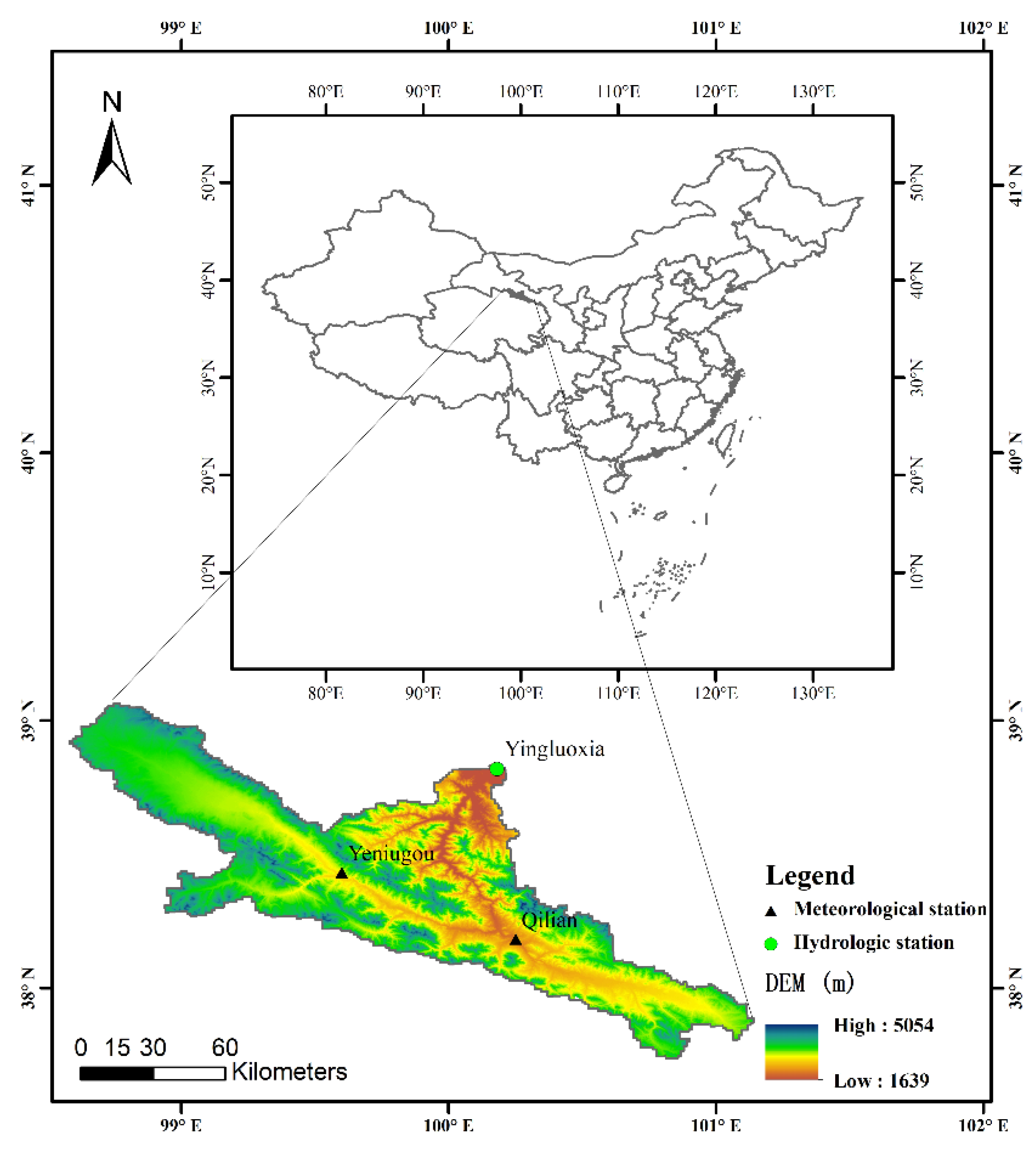
Figure 1. Location of the upper reach of the Heihe River basin in China.
Atmosphere 14 00539 g001
Figure 2. Meteorological data before and after bias correction and historical observations.
Atmosphere 14 00539 g002
Figure 3. Interannual distribution of meteorological data before and after bias correction and historical observations.
Atmosphere 14 00539 g003
Figure 4. Extreme precipitation events before and after bias correction and historical observations. (a) is a scatter plot, and (b) is a box plot.
Atmosphere 14 00539 g004
Figure 5. Box plot of historical and future temperatures and precipitation in the study area.
Atmosphere 14 00539 g005
Figure 6. Boxplot of inter-annual temperatures and precipitation in the historical and future periods in the study area.
Atmosphere 14 00539 g006
Figure 7. Comparison of observed and simulated monthly runoff during the calibration and validation periods.
Atmosphere 14 00539 g007
Figure 8. Comparisons of observed and simulated high flows and low flows. (a) is a scatter plot, and (b) is a box plot.
Atmosphere 14 00539 g008
Figure 9. Comparison of the projected runoff from 2031 to 2070 and the historical runoff from 1961 to 2000.
Atmosphere 14 00539 g009
Figure 10. The inter-annual projected and historical runoffs in the study area.
Atmosphere 14 00539 g010
Figure 11. Box plot of historical and future high flows and low flows.
Atmosphere 14 00539 g011
Figure 12. The estimated return levels of annual mean flows, high flows, and low flows.
Atmosphere 14 00539 g012
Figure 13. The projected mean flows, high flows, and low flows for different return periods.
Atmosphere 14 00539 g013
Table 1. Data used in the study and their sources and descriptions.
Data TypeData SourceSpatial/Temporal ResolutionDescription
DEMThe data set is provided by Geospatial Data Cloud site, Computer Network Information Center, Chinese Academy of Sciences. http://www.gscloud.cn/ (accessed on 26 March 2021).90 mElevation
Land usehttps://doi.org/10.12078/2018070201 (accessed on 19 April 2021).1 kmThe classification system contains 7 categories
Soil typehttps://www.fao.org/soils-portal/soil-survey/soil-maps-and-databases/harmonized-world-soil-database-v12/en/ (accessed on 19 April 2021).1 kmParameters in the soil attribute database were calculated using SPAW and HWSD
Meteorological datahttp://data.cma.cn/site/index.html (accessed on 19 April 2021).DailyGrid and gauge stations
Runoff dataHydrologic manualMonthlygauge station
GCMhttp://www.ceda.ac.uk (accessed on 25 June 2021).DailyCSIRO-MK-3.6.0
Table 2. Locations of meteorological and hydrological stations in the study area.
Station TypeStation NameLongitude (°)Latitude (°)
Hydrological stationYingluoxia38.82100.18
Meteorological stationYeniugou38.4299.58
Qilian38.18100.25
Table 3. Model performance evaluation criteria [46].
Performance Rating N S E R 2
Very Good0.75–1.000.75–1.00
Good0.65–0.750.65–0.75
Satisfactory0.50–0.650.50–0.65
Unsatisfactory<0.50<0.50
Table 4. Statistical values of runoff.
SeriesMean FlowHigh FlowLow Flow
PeriodsBaseline
1961–2000
Future
2031–2070
RC
(%)
Baseline
1961–2000
Future
2031–2070
RC
(%)
Baseline
1961–2000
Future
2031–2070
RC
(%)
Maximum68.0066.45−2202.60229.301316.0826.6065
Minimum32.2432.99279.3467.15−159.2020.20120
Mean47.6251.288138.88134.15−312.3524.2797
Std7.117.921130.6237.14211.761.50−15
Median46.9750.798138.60129.45−711.9624.25103
Range35.7633.46−6123.26162.15326.876.40−7
Cv0.150.1500.220.28270.140.06−57
Table 5. Fitting results from GEV distribution.
Time seriesK-SA-DParameter value
Annual flow (1961–2000)0.0880.269k = −0.18923 s = 6.66 m = 44.848
Annual flow (2030–2070)0.0690.180k = −0.2659 s = 7.9221 m = 48.402
High flow (1961–2000)0.0770.218k = −0.25261 s = 30.813 m = 127.4
High flow (2030–2070)0.1300.490k = −0.169 s = 34.249 m = 119.36
Low flow (1961–2000)0.0990.236k = −0.19532 s = 1.7079 m = 11.646
Low flow (2030–2070)0.0750.260k = −0.47249 s = 1.5974 m = 23.883
Disclaimer/Publisher’s Note: The statements, opinions and data contained in all publications are solely those of the individual author(s) and contributor(s) and not of MDPI and/or the editor(s). MDPI and/or the editor(s) disclaim responsibility for any injury to people or property resulting from any ideas, methods, instructions or products referred to in the content.