Abstract
Global warming is directly related to heavy-duty vehicle fuel consumption and greenhouse gas (CO2 mainly) emissions, which, in China, are certified on the vehicle chassis dynamometer. Currently, vast amounts of vehicle real-road data from the portable emission measurement system (PEMS) and remote monitoring are being collected worldwide. In this study, a binning-reconstruction calculation model is proposed, to predict the chassis dynamometer fuel consumption and CO2 emissions with real-road data, regardless of operating conditions. The model is validated against chassis dynamometer and PEMS test results, and remote monitoring data. Furthermore, based on the proposed model, the fuel consumption levels of 1408 heavy-duty vehicles in China are analyzed, to evaluate the challenge to meet the upcoming China fourth stage fuel consumption limits. For accumulated fuel consumption based on the on-board diagnostic (OBD) data stream, a predictive relative error less than 5% is expected for the present model. For bag sampling results, the proposed model’s accuracy is expected to be within 10%. The average relative errors between the average fuel consumption and the China fourth stage limits are about 3%, 8%, and 0.7%, for current trucks, tractors, and dump trucks, respectively. The urban operating condition, with lower vehicle speeds, is the main challenge for fuel consumption optimization.
1. Introduction
Global warming has become an increasing social concern, which is considered closely related to the greenhouse gases (GHG, e.g., CO2 emissions) generated by human activities, especially since the beginning of industrialization [1]. China has announced its ambition to achieve the ‘carbon peak’ by 2030, and become ‘carbon neutral’ by 2060. To accomplish this goal, CO2 emissions per gross domestic product (GDP) need to be reduced by 65%, and non-fossil energy needs to account for 25% of the primary energy consumption before 2030 [1]. In China, about 10% of the total energy is consumed in the transportation industry, and about half of the CO2 emissions from the transportation industry are generated by heavy-duty vehicles, which account for only 10% of the vehicle population [2]. Over 80% of NOx emissions, and over 90% of particulate matter (PM), come from heavy-duty vehicles in China [3].
In addition, the current European Union’s (EU) climate goal is to reduce net GHG emissions by at least 55% by 2030 (also known as ‘Fit for 55’) [4]. In the latest Euro seventh stage emission regulation proposal [5], a vehicle energy consumption calculation tool (VECTO) is adopted as the simulation tool for determining CO2 emissions and fuel consumption for heavy-duty vehicles. The VECTO was developed by the European Commission, and has been introduced in the European vehicle type-approval regulation since 2017 [6]. Multiple models (including driving cycle, driver, vehicle, wheels, brakes, axle gear, retarder, gearbox, clutch, engine, auxiliaries, etc.) are incorporated, and many input parameters (i.e., rolling resistance, air drag, masses, inertias, gearbox friction, auxiliary power, engine performance, etc.) are needed in the VECTO.
Furthermore, a greenhouse gas reporting program (GHGRP) [7] was launched in the U.S. to collect GHG data and other relevant information from large GHG emission sources, fuel and industrial gas suppliers, and CO2 injection sites. Based on the data from the GHGRP and other sources, the U.S. environmental protection agency (EPA) has prepared the inventory of U.S. GHG emissions and sinks [7] since the early 1990s. In the EPA’s 2027 heavy-duty engine and vehicle standard [8], a greenhouse gas emissions model (GEM) [9] is adopted as a means for determining compliance for emission and fuel efficiency standards. The GEM architecture consists of four systems, i.e., ambient, driver, powertrain, and vehicle. Three drive cycles, including a transient cycle and two cruise speed cycles, are incorporated in the phase two GEM. To accommodate a variety of vehicle-specific information, the input component description files can be modified or adjusted. Although many key parameters, which are either hard to quantify due to lack of certified testing procedures, or difficult to obtain due to propriety barriers, are predefined in the GEM, and a set of user-defined parameters are required for vehicle CO2 emission and fuel consumption calculations.
On the contrary, heavy-duty vehicle fuel consumption is certified using experimental methods in China. The current China third stage fuel limit standard was implemented in 2018 [10], and the corresponding test method standard was updated in 2021 [11]. Recently, a fourth stage fuel limit standard was proposed, with a 10–15% further reduction in fuel consumption for heavy-duty vehicles, and is expected to take effect in 2025. To obtain the vehicle fuel consumption value, the first step is to measure the resistance coefficients by a two-way coasting test in neutral, on a straight road at full vehicle load. Recommended resistance coefficients are also contained in the standard. The second step is to measure CO2 emissions on the chassis dynamometer with the measured or recommended resistance coefficients. In the current fuel consumption standard, an adapted world transient vehicle cycle (C-WTVC), which was developed based on the world harmonized vehicle cycle (WHVC), is utilized, while the test cycle is being updated to the new China heavy-duty commercial vehicle test cycle (CHTC) [12] fourth stage standard. However, only the results from the C-WTVC are to be discussed in this study, since the new test method standard is not implemented yet. The final step is to calculate the weighted type-approval fuel consumption level from CO2 emissions based on the carbon-balance law, using the weighting coefficients shown in Table 1. The C-WTVC comprises three parts: urban, suburb, and highway; heavy-duty vehicles are divided into five categories: trucks, tractors, dump trucks, buses, and urban buses. The weighting coefficients differ for different categories and gross vehicle weights (GVWs), to simulate their common usage scenarios. The fuel consumption limits are in a derated schedule for different GVWs in the individual categories. Details can be found in later sections of this study. Lourenco et al. [13] analyzed the effects of different variables (speed profiles, tire parameters, and rolling resistance coefficients) on the chassis dynamometer fuel consumption measurement, and found that the rolling coefficients were the most influential factors. Wang et al. [14] developed a polynomial model, a black box artificial neural net model, a polynomial neural network model, and a multivariate adaptive regression spline (MARS) model to predict heavy-duty fuel consumption. Among the four model approaches, the MARS model gave the best predictive performance, with an average error of −1.84% over the chassis dynamometer driving cycle.

Table 1.
Weighting coefficients in the China third stage fuel consumption standard.
In the sixth stage of heavy-duty vehicle emission standards across the EU, the U.S., and China, a portable emission measurement system (PEMS) is adopted as a means to obtain real-road emission results. The PEMS test is normally conducted with a specific vehicle load (10–100%) and a specific route (urban, suburb plus highway), and the sampling rate is usually 1Hz. Moreover, the current emission monitoring trend is conducted through wireless data transmission. In the China sixth emission standard [15], remote monitoring is adopted in order to acquire vehicle operating and emission data by 1Hz, over the entire useful life of the vehicle. The EU is considering continuous emissions monitoring in its seventh stage emission standard policy options [16]. The U.S. has already started to require manufacturers to report on-board diagnostic (OBD)-based vehicle operating, NOx, and GHG emission data in its real emission assessment logging (REAL) program [17]. Thus, the vehicle emission and fuel consumption characteristics can be analyzed with these real-road data, and the monitoring efficiency can be increased significantly. Zhang et al. [18] found a good agreement between the remote monitoring and PEMS results, with an average relative error of approximately −15%. Wang et al. [19] developed a platform to effectively monitor urea consumption rationality, injection system working state, exhaust temperature sensor rationality, and NOx emission levels. Yang et al. [20] compared CO2 emissions from conventional diesel and hybrid buses, and found that CO2 emissions were reduced by series-parallel hybrid technology, due to the benefits of the technology under the operating modes of low speed and low power demand.
The above-mentioned real-road data are obtained with different drivers, vehicle loads, road resistances (e.g., water or ice covered), wind speeds, slopes, and other possible conditions, while the vehicle fuel consumption is certified with a specific cycle on the chassis dynamometer, with full load resistance coefficients in China. Effectively evaluating fuel consumption levels, using real-road data, has become a challenge in terms of data analysis. In this work, a binning-reconstruction model is proposed to predict the chassis dynamometer fuel consumption test results with real-road data, regardless of operating conditions. The model is validated against chassis dynamometer and PEMS test results, and remote monitoring data. Additionally, the fuel consumption of 1408 heavy-duty vehicles in China is analyzed using the present model, to evaluate the challenge to meet the proposed China fourth stage fuel consumption limits.
2. Calculation Model
A binning-reconstruction model is proposed in this paper, to predict the heavy-duty vehicle chassis dynamometer fuel consumption or CO2 emissions using real-road data. The model is based on the engine fuel mapping method, which is commonly used in the engine industry, and adopted in the EPA 2027 heavy-duty vehicle and engine emission standard. The model structure is shown in Figure 1 and works as follows:
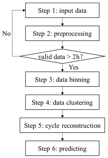
Figure 1.
The binning-reconstruction model.
Step 1: The input data are composed of two parts: the real-road data, and the chassis dynamometer test data (hereinafter referred to as “dynamometer data”). The necessary input data names, and the corresponding data sources, are listed in Table 2. The frequency of all input data should be 1 Hz, which is the same sampling rate of PEMS devices, remote monitoring, and the chassis dynamometer test, according to the China sixth emission standard. For real-road PEMS tests, a vehicle load of more than 30% is recommended in order to cover as much of the engine map as possible.
Table 2.
Input data.
Step 2: For the real-road data, exclude data during the engine shutdown, or when the engine coolant temperature is less than 70 °C. The valid real-road data after exclusion are recommended to be longer than 2 h, otherwise more real-road input data are needed. For the valid real-road data and dynamometer data, calculate the net torque and engine power using the following equations:
where: is the second indexing variable, is the engine net torque output (Nm), is the engine reference torque (Nm), is the engine actual torque (%), is the engine friction torque, is the engine power (kW), is the engine speed (r/min).
Step 3: (a) Torque binning: choose an appropriate torque bin interval () based on the engine reference torque, or use the following equation to calculate . A range of 20–200 Nm is recommended, which is close to the engine calibration interval.
Label each second of the valid real-road data and the dynamometer data with a number , which is calculated using:
(b) Engine speed binning: choose an appropriate engine speed bin interval () based on the maximum engine speed (), or use the following equation to calculate . A range of 50–200 Nm is recommended, which is close to the engine map calibration interval.
Label each second of the valid real-road data and the dynamometer data with a number , which is calculated using:
Step 4: All the fuel consumption data in the valid real-road data with a label of and , cluster as a set (. If the element number in is less than or equal to 5, exclude this in the following calculation. For with an element number larger than 5, calculate the set’s average value () and standard deviation (). Exclude the elements in which are less than or larger than assuming that obeys the normal distribution. Calculate the average value () of the rest of the elements in .
Step 5: After Step 3, each second of the dynamometer data is also labelled with . The chassis dynamometer fuel consumption rate () curve could be predicted with the real-road data as:
If the corresponding does not exist for a specific , a one-dimensional (1D) or a two-dimensional (2D) fitting method may be performed to predict the missing value, as discussed in Section 4.2 of this paper. The CO2 emission rate () could be predicted based on the carbon balance law:
where: is the diesel density (g/L).
Step 6: (a) CO2 aligning: Compared to the engine real-time data stream, the CO2 measurement could be delayed for up to 8 s due to the gas transmission in this study (see Section 4.4). Therefore, , which is predicted using the real-time OBD fuel consumption rate, needs to be aligned with the experimental CO2 emission rate () in order to accurately predict the bag sampling results. Calculate the correlation coefficients () of and from = 1 s to = 20 s with an increasing step of 1 s, where “” means the data starting () and ending time (), and is the data length of the dynamometer data. Find the maximum value of and the corresponding . Thus, the delay time equals and the aligned results for are where 1 ≤ ≤ ≤ .
(b) Predicting the chassis dynamometer test results: the experimental (, g/kWh) and predicted (, g/kWh) duty cycle CO2 emissions could be calculated by:
The bag sampling-based fuel consumption (, L/100km) for a specific cycle part (urban, suburb, or highway) could be predicted using:
where: and are the starting time and ending time of this cycle part, respectively. is the vehicle speed in dynamometer data (km/h).
To evaluate the predicted results, relative errors (, %) between the calculated results and experimental data are calculated by:
where: and are calculated and experimental results for fuel consumption or CO2, respectively.
3. Experimental Setup
The proposed binning-reconstruction model is validated against experimental and monitoring data from four China 6th stage emission heavy-duty vehicles. The vehicle specifications and data sources are listed in Table 3. Vehicles 1 and 2 cover the daily route (random traffic conditions), while vehicles 2 and 3 cover the PEMS test driving condition. As for vehicle 4, 1 Hz remote monitoring data, about 106.6 h, are used as real-road input data. Note that the input remote monitoring data does not need to be on this scale, as long as the valid input data are longer than 2 h, as previously mentioned.
Table 3.
Vehicle specifications and data sources.
The real-road tests were conducted with a HORIBA OBS-ONE PEMS device, which is able to record CO2, CO, NOx, and PN emissions, as well as engine data streams, through the OBD connector at 1Hz. The CO2 and CO measurements were performed by the non-dispersive infrared (NDIR) analyzer in the PEMS device.
The fuel consumption and CO2 emissions were tested on a MAHA CDM-72HDD-4WD heavy-duty chassis dynamometer, whose roller diameter is about 1.8 m. The emission measurement was conducted using a HORIBA MEXA-7200DTR constant volume sampler (CVS). The CO2 and CO measurements were also based on NDIR. The CVS is equipped with 4 sampling bags, the maximum volume of which is 120 L. As shown in Figure 2, the C-WTVC driving cycle, which was developed in the China 3rd stage fuel consumption standard, was utilized for all four vehicles. The C-WTVC lasts 1800 s in total, and consists of three parts, each representing urban, suburb, and highway roads. Note that the calculation model can also be applied for other driving cycles, such as CHTC, etc.
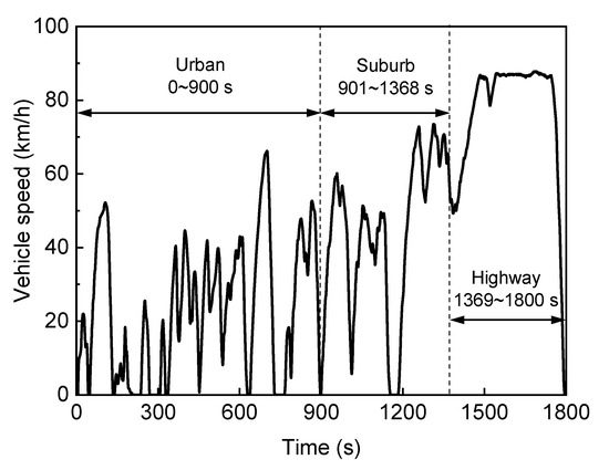
Figure 2.
The adapted world transient vehicle cycle (C-WTVC).
4. Results and Discussion
4.1. Feasibility of the Binning-Reconstruction Model
The simulation results of vehicle one are shown in this section, to prove the feasibility of the proposed binning-reconstruction model. Two cases are studied: case one, with a of 100 r/min and a of 25 Nm (hereinafter referred to as “n100T25”), and case two, with a of 50 r/min and a of 20 Nm (hereinafter referred to as “n50T20”). Figure 3 shows the average fuel rate and standard deviation for each valid bin in n100T25 and n50T20. A total of 172 bins are generated in n100T25, while 385 bins are generated in n50T20. As can be seen, a more comprehensive fuel consumption map can be obtained with smaller bin intervals. However, this does not necessarily mean that the simulation results are more accurate, since the element number in each bin decreases as well. The effects of bin interval are discussed in detail in Section 4.3. It can be seen that the bin distributions of the average fuel rate, of both cases, are able to capture the engine fuel consumption map; in other words, the fuel consumption rate increases as the engine speed and torque increase. As for the fuel rate standard deviation, most bins are found to be less than 0.5 L/h, indicating that the clustering extent of elements in these bins is satisfying, since this binning method is based on the engine mapping. The standard deviation in two specific areas, the medium engine speed and medium-high torque area, and the high engine speed and low torque area, are found to be higher than the rest of the areas in both cases. The highest fuel rate standard deviation, of 4.4 L/h, was located in the bottom right corner (engine speed = 2250–2300 r/min, torque = 0–20 Nm) in n50T20. High standard deviation is believed to be caused by unstable engine operation in these areas. To combat this adverse effect, bins with insufficient elements (≤five) are excluded from calculation, as described above, and a 2D fitting method is coupled (see the next section).
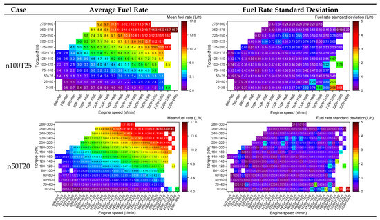
Figure 3.
Binning of the fuel rate (vehicle one).
To further understand the clustering level of this binning method, engine speed cross-sections and torque cross-sections of the bin distribution in Figure 3 are shown in Figure 4, intersecting at the medium engine speed and medium-high torque area, where the standard deviation is relatively higher. The number of elements in each bin is also illustrated. By decreasing the bin interval from n100T25 to n50T20, it can be seen that the data number curves are similar for both cross-sections, with a decrease of the data number in each bin. Note that the data number curve shape is mainly influenced by the input real-road data. Therefore, higher vehicle loads (>30%) and a minimum valid data length (>2 h) are recommended, in order to ensure that enough elements are included in each bin, as described in the model introduction. For the engine speed cross-sections in both cases, reasonable data clustering can be observed, with an interquartile range (IQR, the distance between the upper and lower quartiles) no more than 1 L/h for most bins. For the torque cross-sections in both cases, although a relatively large data range of about 4 L/h can be noted for the medium engine speed bins, resulting in the high standard deviations shown in Figure 3, the IQR is no more than 1.5 L/h for most bins. Furthermore, the little difference between the median line and average values supports the assumption that elements in each bin obey approximate normal distribution. To conclude, the average fuel consumption rate in each bin should be able to capture the real-world engine fuel consumption rate to some extent.
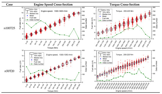
Figure 4.
Clustering of the fuel rate bins (vehicle 1).
After obtaining the average fuel consumption rate for each bin, the chassis dynamometer test process can be reproduced, or “reconstructed”, by matching the torque bin number and the engine speed bin number second by second, as presented in Figure 5. It is noteworthy that the predicted or “reconstructed” fuel rate curve yields good agreement with the experimental results. The relative errors between the predicted accumulated fuel consumption over the driving cycle and measurements are 1.42% and 1.70% for n100T25 and n50T20, respectively, validating the feasibility of the proposed binning-reconstruction model.
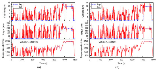
Figure 5.
Reconstruction of the chassis dynamometer cycle (vehicle one). (a) n100T25. (b) n50T20.
4.2. Predicting the Unknown Point
As described in Section 2, sometimes the input data binning fails to cover some operation points in the chassis dynamometer cycle. In that case, the unknown points need to be predicted based on the given data, using two following fitting methods:
- (a)
- 1D fitting. The so-called “1D fitting” is based on linear interpolation or extrapolation. Assume that the unknown point is labelled with . If the number of known bins labelled with the same is larger than two, the unknown point is calculated as the interpolated or extrapolated value at of the 1D function, fitted by all known bins labelled with . Otherwise, the unknown data is calculated as the interpolated or extrapolated value at of the 1D function, fitted by all known bins labelled with .
- (b)
- 2D fitting. The so-called “2D fitting” is based on 2D interpolation or extrapolation. A surface function can be fitted using all the known bins, as shown in Figure 6. Then, unknown points can be calculated as the interpolated or extrapolated value at of this surface function.
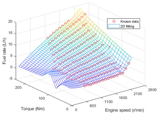 Figure 6. Two-dimensional fitting to predict unknown data (vehicle one, n100T25).
The predicted and experimental result relative error absolute values, using the 1D and 2D fitting method, for vehicles one to four, are compared in Figure 7. The relative error is calculated based on the accumulated fuel consumption over the driving cycle, and the test data from the engine OBD data stream. It can be observed that in most cases, the 2D fitting method produces lower or comparable relative errors with the 1D fitting method. Given that the 2D fitting method is not necessarily more computationally expensive, since the surface function only needs to be generated once, while the 1D fitting needs to be conducted every time when an unknown point is encountered, the 2D fitting method is recommended in this model, and is used in the following study.
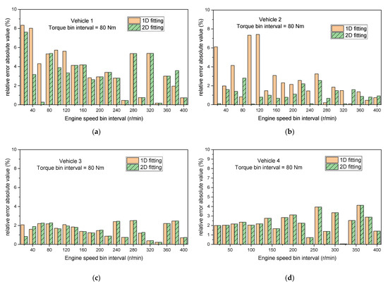
Figure 7.
Relative error absolute value differences between 1D and 2D fitting. (a) Vehicle one. (b) Vehicle two. (c) Vehicle three. (d) Vehicle four.
4.3. Effects of the Binning Interval
Another important factor influencing the model accuracy is the bin interval. The relative error matrices over a torque and engine speed bin interval sweep, for vehicles one to four, are presented in Figure 8. As could be noticed from the bottom left corners of Figure 8a,b, if the torque and engine speed bin intervals are simultaneously too small, so that insufficient elements are included in each bin, causing inaccurate fuel consumption mapping, the relative error seems to increase. As the torque bin interval (see the upper part) or the engine bin interval (see the right part) increases, the total bin number decreases, resulting in increasing accuracy loss and relative error. Generally speaking, a of 20–200 Nm, and a of 50–200 r/min, which is close to the engine mapping calibration interval, are recommended for this model, as mentioned above. Note that similar torque and engine speed setpoint intervals are used in the steady-state fuel-mapping test procedure in the EPA’s 2027 motor vehicle emission standard [8]. It is very interesting to note that in this area ( = 20–200 Nm and = 50–200 r/min), the relative error seems not to be sensitive to or . A relative error of less than 5% for the accumulated fuel consumption prediction over the driving cycle is expected to be achieved using the proposed model.
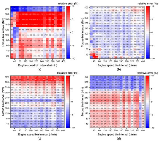
Figure 8.
Effects of the binning interval (2D fitting). (a) Vehicle one. (b) Vehicle two. (c) Vehicle three. (d) Vehicle four.
4.4. Predicting the Bag Sampling Results
As previously mentioned, in China the fuel consumption certification test is conducted on the chassis dynamometer using the CVS bag sampling method, and the present model aims at predicting these results.
Figure 9 shows the curve (see Section 2) over the delay time . It is noted that for vehicles two, three, and four, the emission analyzer delay time is = 8 s, which is nearly 2% of the highway part (431 s) and is, therefore, non-negligible compared to the accuracy of the present model.
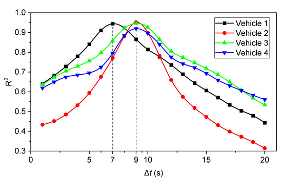
Figure 9.
The correlation coefficient vs. delay time.
For vehicle one, the experimental delay time is found to be = 6 s. The CO2 rates before and after aligning are shown in Figure 10. It is demonstrated that the current method, used to calculate the curves, works reasonably well to define the delay time.
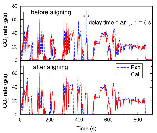
Figure 10.
Experimental and calculated CO2 rate, before and after aligning (vehicle one).
Table 4 shows the measured and predicted CO2 emissions and fuel consumptions for each cycle part, and their weighted (see Table 1 for the weighting coefficients) and accumulated results. It is indicated that the present model yields acceptable agreement for both CO2 and fuel consumption for each bag sampling measurement, and their weighted and accumulated results. The highest relative error (−8.2%) is found for the highway CO2 emission predicting, which is thought to be caused by the testing uncertainty, or the fuel consumption calibration error. Note that the CO2 emission and fuel consumption predicting is based on the engine OBD fuel consumption data stream, which is calculated from the engine look-up tables, that is to say, engine maps. The engine fuel consumption maps are calibrated in a laboratory and pre-written into the engine control unit. Therefore, some system errors may be generated during the engine map building process. It is safe to say that the present model’s accuracy is within 10% for bag sampling predicting. Furthermore, it is interesting to note that the present model is able to predict the chassis dynamometer results with different vehicle load resistance coefficients, as can be seen from the results of vehicle four.
Table 4.
Experimental and calculated results, and the relative error.
4.5. Heavy-Duty Vehicle Fuel Consumption
In the China third stage fuel consumption standard, heavy-duty vehicles are divided into five categories: trucks, tractors, dump trucks, buses, and urban buses, as indicated in Table 1. Derated limits for fuel consumption are adopted based on the vehicle’s GVW. Using the present calculation model, 1408 heavy-duty vehicles’ certification fuel consumption levels are predicted using real-road data, including PEMS tests and remote monitoring data. The number of investigated vehicles in different GVW bins for each category are presented in Figure 11. It is obvious that most vehicles are from the truck, tractor, and dump truck categories. On the contrary, the number of vehicles in the bus and urban bus categories is relatively small, due to fact that type-approval applications for these categories are rare in China. However, the authors decided to demonstrate these predicted results for the bus and urban categories, considering that it would be interesting to compare them with other categories.
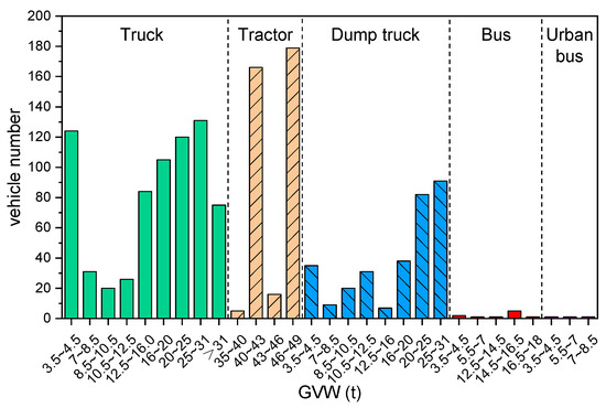
Figure 11.
The number of vehicles included in this investigation.
Figure 12 shows the calculated fuel consumption for each vehicle, and the corresponding derated limits in the China third and upcoming fourth stage heavy-duty fuel consumption standards. For all the investigated vehicles, the predicted fuel consumption is within the current China third stage limits, which is not surprising, since most vehicles are manufactured, provided, and kept in the type-approval level. Nevertheless, some vehicles fail to meet the fourth stage limits, suggesting that further efforts are needed to reduce fuel consumption levels. The average fuel consumption of small GVW vehicles is near the fourth stage limits, while large gaps (nearly 2.5 L/100 km) are identified for larger GVW (over 20 t) vehicles in the truck, tractor, and dump truck categories. It is also of interest to note that the fuel consumption limits are to be increased for buses over 12.5 t. These increasing limits are adopted taking into account that the type-approval test cycle is changing from C-WTVC to CHTC, which is found to be unfavorable for fuel consumption for specific vehicle types. By comparing fuel consumption limits for the same GVW, it is revealed that the dump truck limits are higher than the truck limits, while the urban bus limits are higher than those of buses. This is due to the fact that urban vehicles, such as dump trucks and urban buses, are usually operated at lower speeds, resulting in higher fuel consumption levels. This is the reason why these vehicles are treated as separate categories.
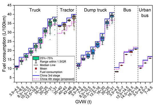
Figure 12.
Fuel consumption distributions, and the China third and fourth stage limits.
To further understand the fuel consumption reduction challenge, relative errors between average fuel consumption and the upcoming China fourth stage limits are shown in Figure 13. Note that the bus and urban bus categories are not included this time, because of the small sample size. It is observable that some negative values are found for small GVW vehicles. However, the situation is not optimistic, considering the challenge of the new test cycle (CHTC). The highest relative errors, up to 11.2%, are found for tractors between 35 t and 40 t, and the average relative error for tractors is around 8%. The average relative errors for trucks and dump trucks are around 3% and 0.7%, respectively. As previously discussed, the prediction accuracy of the present model is within 10%, which is comparable to the relative error level presented in Figure 13. However, this should be negligible, since the prediction uncertainties are believed to be somewhat normalized or remoted during the averaging process.
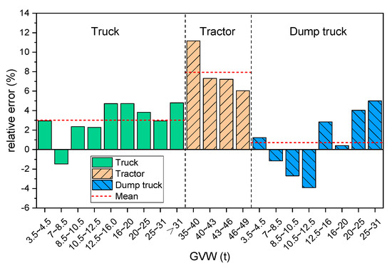
Figure 13.
Relative errors between average fuel consumption and the China fourth stage limits.
The fuel consumption levels of different cycle parts (urban, suburb, and highway), for trucks and tractors, are shown in Figure 14 and Figure 15, respectively. Note that the certified fuel consumption is calculated by weighting the three individual cycle parts with different weighting coefficients. Thus, dump trucks are not analyzed this time since their urban:suburb:highway ratio is 0:100%:0. As can be seen from Figure 14, the highway part ratio increases from 20% to 60%, while the urban part ratio declines from 40% to 10% as the GVW increases, which is consistent with the daily route of trucks with different GVWs. As expected, the fuel consumption of the urban part is about 20% higher than that of the suburb part, and about 50% higher (when GVW > 20 t) than that of the highway part. Therefore, the urban operating condition, with lower vehicle speeds, is the main challenge for fuel consumption optimization. It is interesting to note that the highway part fuel consumption is slightly higher than the suburb part for trucks with a GVW lower than 10.5 t. This is because the engine displacements for trucks with lower GVWs are normally small. Consequently, the engine has to operate with a richer fuel-air mixture, i.e., at the poor fuel economy region, when high power outputs are needed in the highway operating condition, with vehicle speeds higher than 80 km/h. For trucks with a GVW over 10.5 t, fuel consumption reduction for suburb roads becomes the second priority. The fuel consumption for all three parts experiences an upward trend as the GVW rises, leading to overall increasing fuel consumption, as shown in Figure 15.
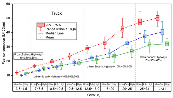
Figure 14.
Fuel consumption of different cycle parts (truck).
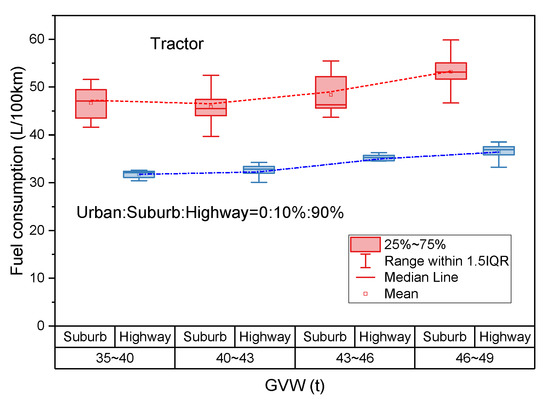
Figure 15.
Fuel consumption of different cycle parts (tractor).
For tractors, only the suburb and highway parts are included in the weighted fuel consumption calculation. The GVWs of the investigated tractors without trailers are no less than 35 t. Although the fuel consumption of the highway part is about 50% lower than that of the suburb part for all GVW bins, it still needs to be kept in mind because the ratio for this part is up to 90%. Generally speaking, tractors are facing a great challenge in meeting the future China fourth fuel consumption standard, with an average relative error of 8%, as discussed previously.
5. Conclusions
To predict the heavy-duty chassis dynamometer fuel consumption and CO2 emissions with real-road data, a binning-reconstruction model is described in this study. The feasibility of the proposed model, the fitting methods to predict unknown points, the effects of the binning interval, and the prediction of bag sampling results are further investigated. Finally, the fuel consumption performances of 1408 heavy-duty vehicles in China are analyzed to evaluate the challenge to meet the upcoming China fourth stage fuel consumption standard. The conclusions can be summarized as follows:
The binning of real-road fuel consumption, based on torque and engine speed, is good enough to capture the engine fuel consumption mapping. The 2D fitting method is recommended to predict the unknown data. A torque bin interval of 20–200 Nm and an engine speed bin interval of 50–200 r/min are recommended for this model, since a bin interval too large or too small would cause an increase in the predicting error. For cycle accumulated fuel consumption based on the OBD data stream, a relative error less than 5% for prediction is expected to be achieved, using the proposed model. For bag sampling results, the present model accuracy is expected to be within 10%.
For dump trucks and urban buses, which are mainly operated at lower speeds, the average fuel consumption levels are found to be higher than those of trucks and buses with the same GVWs. The average relative errors between the average fuel consumption and the China fourth stage limits are about 3%, 8%, and 0.7%, for trucks, tractors, and dump trucks, respectively. The urban part fuel consumption is about 20% higher than the suburb part, and about 50% higher than the highway part for trucks with a GVW > 20t. Thus, the urban operating condition with lower vehicle speeds is the main challenge for fuel consumption optimization for trucks.
Author Contributions
Conceptualization, G.L. and S.R.; methodology, S.R.; software, S.R.; validation, Z.L., X.W. and D.G.; formal analysis, S.R.; investigation, S.R.; resources, X.L.; data curation, Z.L.; writing—original draft preparation, S.R.; writing—review and editing, S.R.; visualization, S.R.; supervision, T.L.; project administration, H.L.; funding acquisition, X.L. All authors have read and agreed to the published version of the manuscript.
Funding
This research received no external funding.
Institutional Review Board Statement
Not applicable.
Informed Consent Statement
Not applicable.
Data Availability Statement
Not applicable.
Conflicts of Interest
The authors declare no conflict of interest.
References
- Shijin, S.; Zhi, W.; Xiao, M.; Hongming, X.; Xin, H.; Jianxin, W. Low carbon and zero carbon technology paths and key technologies of ICEs under the background of carbon neutrality. J. Automot. Saf. Energy 2021, 12, 417–439. [Google Scholar] [CrossRef]
- He, J. Research on China’s long-term low-carbon development strategy and transformation path. China Popul. Resour. Environ. 2020, 30, 1–25. [Google Scholar] [CrossRef]
- Ministry of Ecology and Environment of the P.R.C. China Mobile Source Environmental Management Annual Report; Ministry of Ecology and Environment of the P.R.C.: Beijing, China, 2022. Available online: https://www.mee.gov.cn/ywdt/xwfb/202212/t20221207_1007157.shtml (accessed on 10 February 2023).
- Fit for 55. Available online: https://www.consilium.europa.eu/en/policies/green-deal/fit-for-55-the-eu-plan-for-a-green-transition (accessed on 10 February 2023).
- Euro 7; Proposal for a Regulation of the European Parliament and of the Council on Type-Approval of Motor Vehicles and Engines and of Systems, Components and Separate Technical Units Intended for such Vehicles, with Respect to their Emissions and Battery Durability (Euro 7) and Repealing Regulations (EC) No 715/2007 and (EC) No 595/2009. The European Commission: Brussels, Belgium; The European Union: Brussels, Belgium, 2022.
- Vehicle Energy Consumption Calculation Tool—VECTO. Available online: https://climate.ec.europa.eu/eu-action/transport-emissions/road-transport-reducing-co2-emissions-vehicles/vehicle-energy-consumption-calculation-tool-vecto_en (accessed on 10 February 2023).
- The United States Environment Protection Agency (EPA). 2021 GHGRP Overview Report; The United States Environment Protection Agency (EPA): Washington, DC, USA, 2022. Available online: https://www.epa.gov/ghgreporting/ghgrp-yearly-overview (accessed on 10 February 2023).
- 40 CFR; Control of Air Pollution from New Motor Vehicles: Heavy-Duty Engine and Vehicle Standards. The United States Environment Protection Agency (EPA): Washington, DC, USA, 2022.
- Greenhouse Gas Emissions Model (GEM) v4.0 User Guide. Available online: https://www.epa.gov/regulations-emissions-vehicles-and-engines/greenhouse-gas-emissions-model-gem-medium-and-heavy-duty#overview (accessed on 10 February 2023).
- GB 30510-2018; Fuel Consumption Limits for Heavy-Duty Commercial Vehicles. Standards Press of China: Beijing, China, 2018.
- GB/T 27840-2021; Fuel Consumption Test Methods for Heavy-Duty Commercial Vehicles. Standards Press of China: Beijing, China, 2021.
- Yu, H.; Liu, Y.; Li, J.; Ma, K.; Liang, Y.; Xu, H. Investigations on fuel consumption characteristics of heavy-duty commercial vehicles under different test cycle. Energy Rep. 2022, 8, 102–111. [Google Scholar] [CrossRef]
- Lourenço, M.A.D.M.; Eckert, J.J.; Silva, F.L.; Miranda, M.H.R.; de Alkmin e Silva, L.C. Uncertainty analysis of vehicle fuel consumption in twin-roller chassis dynamometer experiments and simulation models. Mech. Mach. Theory 2023, 180, 105126. [Google Scholar] [CrossRef]
- Wang, L.; Duran, A.; Gonder, J.; Kelly, K. Modeling heavy/medium-duty fuel consumption based on drive cycle properties. In Proceedings of the SAE 2015 Commercial Vehicle Engineering Congress (COMVEC), Rosemont, IL, USA, 6–8 October 2015. [Google Scholar]
- GB 17691-2018; Limits and Measurement Methods for Emissions from Diesel Fuelled Heavy-Duty Vehicle (China VI). Standards Press of China: Beijing, China, 2018.
- The European Commission. Commission Staff Working Document: Impact Assessment Report Accompanying the Document Proposal for a Regulation of the European Parliament and of the Council (Euro 7) Part1/3; The European Commission: Brussels, Belgium, 2022; Available online: https://single-market-economy.ec.europa.eu/publications/euro-7-standard-proposal_en (accessed on 1 February 2023).
- The California Air Resources Board. California Code of Regulations; The California Air Resources Board: Sacramento, CA, USA, 2019; Section 1971.1, Title 13.
- Zhang, S.; Zhao, P.; He, L.; Yang, Y.; Liu, B.; He, W.; Cheng, Y.; Liu, Y.; Liu, S.; Hu, Q.; et al. On-board monitoring (OBM) for heavy-duty vehicle emissions in China: Regulations, Early-stage Evaluation and Policy recommendations. Sci. Total Environ. 2020, 731, 139045. [Google Scholar] [CrossRef] [PubMed]
- Wang, T.; Liu, J.; Wan, C.; Wang, Z. Remote supervision strategy based on in-use vehicle OBD data flow. E3S Web Conf. 2021, 268, 01007. [Google Scholar] [CrossRef]
- Yang, L.; Zhang, S.; Wu, Y.; Chen, Q.; Niu, T.; Huang, X.; Zhang, S.; Zhang, L.; Zhou, Y.; Hao, J. Evaluating real-world CO2 and NOx emissions for public transit buses using a remote wireless on-board diagnostic (OBD) approach. Env. Pollut. 2016, 218, 453–462. [Google Scholar] [CrossRef] [PubMed]
Disclaimer/Publisher’s Note: The statements, opinions and data contained in all publications are solely those of the individual author(s) and contributor(s) and not of MDPI and/or the editor(s). MDPI and/or the editor(s) disclaim responsibility for any injury to people or property resulting from any ideas, methods, instructions or products referred to in the content. |
© 2023 by the authors. Licensee MDPI, Basel, Switzerland. This article is an open access article distributed under the terms and conditions of the Creative Commons Attribution (CC BY) license (https://creativecommons.org/licenses/by/4.0/).