Synoptic and Mesoscale Analysis of a Severe Weather Event in Southern Brazil at the End of June 2020

Abstract

At the end of June 2020, an explosive extratropical cyclone was responsible for an environment in which a squall line developed and caused life and economic losses in Santa Catarina state, southern Brazil. The aims of this case study are the following: (a) to describe the drivers of the cyclogenesis; (b) to investigate through numerical simulations the contribution of sea–air interaction to the development of the cyclone as an explosive system; and (c) to present the physical properties of the clouds associated with the squall line. The cyclogenesis started at 1200 UTC on 30 June 2020 on the border of southern Brazil and Uruguay, having a trough at middle-upper levels as a forcing, which is a common driver of cyclogenesis in the studied region. In addition, the cyclone’s lifecycle followed Bjerknes and Solberg’s conceptual model of cyclone development. A special feature of this cyclone was its fast deepening, reaching the explosive status 12 h after its genesis. A comparison between numerical experiments with sensible and latent turbulent heat fluxes switched on and off showed that the sea–air interaction (turbulent heat fluxes) contributed to the cyclone’s deepening leading it to the explosive status. The cold front, which is a component of the cyclone, favored the development of a pre-frontal squall line, responsible for the rough weather conditions in Santa Catarina state. While satellite images do not clearly show the squall line located ahead of the cold front in the cyclone wave due to their coarse resolution, radar reflectivity data represent the propagation of the squall line over southern Brazil. On 30 June 2020, the clouds in the squall line had more than 10 km of vertical extension and a reflectivity higher than 40 dBZ in some parts of the storm; this is an indicator of hail and, consequently, is a required condition for storm electrification. In fact, electrical activity was registered on this day.

1. Introduction

At 1200 UTC on 30 June 2020, a cyclogenesis developed on the border of southern Brazil and Uruguay near the southwestern South Atlantic Ocean and in 12 h evolved into an explosive extratropical cyclone, over the ocean, following the methodology of Sanders and Gyakum (1980) [1] and Zhang et al. (2017) [2]. While the center of the cyclone was over the ocean during its entire lifecycle (except during the genesis), the cold front associated with the cyclone displaced to the northeast over the continent, crossing extreme southern Brazil and affecting the state of Santa Catarina (SC; Figure 1). The cold front created a favorable environment for the development of mesoscale convective systems, which were directly responsible for a severe weather episode (strong winds and heavy rain) in SC causing a lot of damage such as unroofing, falling trees, and eleven deaths [3,4]. According to the Civil Defense of SC, this event caused the strongest winds and the worst disaster registered so far in the state [5]. The reports of this system by the local Civil Defense and the media to society suggested that the center of the cyclone was over SC, which was a misinterpretation. Due to this fact, the population of SC has developed a strong negative reaction to the word cyclone. In addition, given that the southern Brazilian coast is one of the three cyclogenetic areas on the east coast of South America [6,7,8,9,10], the cyclone word is frequently mentioned by the media during weather forecasts, and it can lead to psychological stress in the population. Hence, we highlight the importance of correct communication of atmospheric systems to society by the media and local authorities.

The previous paragraph introduced the terms extratropical cyclones, explosive extratropical cyclones, mesoscale convective systems, and severe weather, but what are their meanings and how are they connected? Extratropical cyclones are synoptic-scale systems since they have a dimension of ~10³ km and a mean lifetime of three days [9,11,12]. These systems are characterized by a low-pressure center connected to a cold and warm front. In the southeast coast of South America (Uruguay and southern Brazil), the main dynamic driver of extratropical cyclones is a middle-upper level trough traveling from the Pacific to the Atlantic Ocean [7,13,14,15,16,17,18,19,20,21]. Other factors contributing to cyclogenesis in southeastern South America are the jet stream over this region, especially during the winter [20], and the presence of the Andes Mountains, which promote a semi-stationary wave with its trough located near Uruguay [14,22,23]. Hence, when there is a coupling of the semi-stationary trough with the transient disturbances, it strengthens the development of low-level cyclones.

When an extratropical cyclone registers a fast deepening, i.e., a drop in mean sea level pressure equal to or more than 24 hPa (geostrophically adjusted to latitude 60°) within 24 h, it can be considered an explosive cyclone. This definition was firstly introduced by Bergeron and, posteriorly, adapted by Sanders and Gyakum [1]. More recently, Zhang et al. [2] adjusted the definition considering a latitude of 45° and set the threshold to 12 hPa within 12 h. Explosive extratropical cyclones are more frequent over mid-latitude oceans and in the cold season [18,23]. In addition, cyclogenesis density ranges from 40° to 50° S in autumn and winter, and from 50° to 60° S in spring and summer [11,13]. Near the east coast of South America, explosive cyclones occur south of 27° S [23,24].

There is more than one explanation for the fast deepening of the central pressure in some extratropical cyclones. It has been suggested that the baroclinic instability in these systems can be strengthened by different processes such as latent heat release by cloud condensation processes [24,25,26] and the ocean–atmosphere interaction through turbulent heat fluxes [27,28,29]. Latent heat release by condensation processes is important for increasing air instability and decreasing pressure on the surface. Ocean–atmosphere coupling can also intensify the air moisture and, consequently, the heat release by condensation. Neiman and Shapiro [28], for instance, describe that latent and sensible heat fluxes from warm currents may exceed 1000 W m⁻² near the center of the cyclones during their development stage. Kouroutzoglou et al. [30] in a case study of an explosive cyclone over the Mediterranean Sea showed that the system occurred as a result of the downward intrusion of high-potential vorticity cold stratospheric air into the upper troposphere combined with a low-level warm. This warm was a response of positive surface sensible and latent heat fluxes propitiated by the displacement of a cold air mass over the warmer sea. The role of thermodynamic processes in explosive cyclone development has been documented in several ocean basins [30,31,32,33]. However, near the eastern coast of South America, there are few studies about the explosive cyclone’s physics. For instance, through numerical experiments, Dal Piva et al. [31] and Seluchi and Saulo [33] showed that surface heat fluxes and latent heat release by convectionare the main mechanisms acting in cyclone deepening.

Different studies [26,30,34,35,36,37,38,39,40] indicate that explosive cyclones, in general, acquire this feature when their development follows the Shapiro and Keyser [34] conceptual model of cyclone development instead of the classical model of Bjerknes and Solberg [41]. The upper-level flow can be used to estimate the type of frontal structure associated with a mid-latitude cyclone [35]. In Shapiro and Keyser’s model, a cyclone develops in an upper-level confluent background, which contributes to a zonally oriented cyclone (strong warm front, bent-back warm front, and warm seclusion), since the confluent flow stretches the cyclone in the zonal direction. In the case of Bjerknes and Solberg’s model, baroclinic perturbations occur in an upper-level diffluent background, which contributes to a meridionally oriented cyclone (strong cold front, and occlusion) since the diffluent flow stretches the cyclone in the meridional direction. As the warm seclusion in Shapiro–Keyser cyclones is a response to a large latent heat release, the diabatic processes provide an appropriate environment to help the rapid deepening of the cyclones leading to the explosive status [26,37,38,39,40].

Synoptic scale systems provide adequate environmental conditions (supply of moist and warm air, and a lifting mechanism) for the development of mesoscale convective systems [42,43,44,45,46], which are systems with horizontal dimensions from a few to several hundred kilometers and duration from hours to one day [12,45,47]. Mesoscale convective systems can be a single convective cell or a cluster of clouds organized in lines (squall lines) or a near-circular format (mesoscale convective systems). They are responsible for severe weather, which can produce heavy rain, severe winds, hail, lightning, and tornadoes [12,48,49].

In the presence of thermodynamic instability, a source of additional lifting by a favorable synoptic-scale environment may trigger deep convection (e.g., McNulty [50]). The deep convection, which is thermally driven by turbulent mixing that displaces air parcels from the lower atmosphere to the troposphere above 500 hPa, leads to the development of convective storms [46]. Then, a combination of moist air, a lifting mechanism, and atmospheric instability are the main ingredients for the development of mesoscale convective systems. Moreover, the severity of deep convection is modulated by the relationship between instability and the vertical wind shear [51,52]. Many of the mesoscale convective systems in southeastern South America develop in association with a synoptic environment [19,53,54,55].

For a mesoscale convective system to produce severe weather, it is necessary to develop severe thunderstorms. Although all thunderstorms need the same mentioned ingredients for development, only a small fraction of them becomes severe. It is associated to the fact that the atmosphere needs to have an optimal relationship between instability, which can be measured by the convective available potential energy (CAPE), and vertical wind shear at 0–6 km [56,57,58]. CAPE is an estimate of the vertically integrated buoyancy of adiabatically lifted air, embracing requirements for moisture and instability. Vertical wind shear guides the circulation inside the clouds avoiding the cancellation between downdraft and updraft air. In the case of weak vertical wind shear, there is a cancellation of the vertical circulations inside the clouds and, when there is a very strong vertical wind shear, the clouds do not organize because the droplets are transported far away by wind. Hence, it prevents the cloud development.

Mesoscale convective systems exhibit a variety of cloud and precipitation structures [59], which, in general, are related to the synoptic-scale environment in which they are embedded. Considering the mid-latitude squall lines, this kind of system develops in the warm sector of an extratropical cyclone, often 200–300 km ahead of the surface cold front [60]. There is warm (and moisture) conveyor-belt air (low-level jet) that flows almost parallel to the cold front in the direction of the warm front [61]. As this air flows at lower levels, aloft, in the middle troposphere, there is a westerly dry flow. The described situation is a trigger for potential instability which is associated with convection, and, consequently, with the squall line formation [60]. These two flows also provide the necessary vertical shear of the horizontal wind for squall-line maintenance [62].

Explosive extratropical cyclones and squall lines have long been a focus of several studies but not the association to each other, and mainly over South America and the South Atlantic Ocean. Moreover, the evolution of an extratropical cyclone to the status of explosive continues to be a challenge for weather forecasting since the physical mechanisms are not totally clear and, generally, atmospheric models failing in forecasting these systems. In addition, the physical properties of mid-latitude squall lines in Brazil deserve more attention since these systems have a great potential for destruction. Another point is that the threat of explosive cyclones to maritime traffic safety [63,64,65,66,67,68,69] and coastal areas [23,69,70] does not receive much attention. Therefore, the main goals of this study are (a) to describe the drivers of the cyclogenesis; (b) to investigate the contribution of the sea-air interaction to the development of the cyclone as an explosive system through numerical experiments; and (c) to present the physical properties of the clouds associated with the mesoscale system responsible for the severe weather in SC at the end of June 2020.

2. Materials and Methods

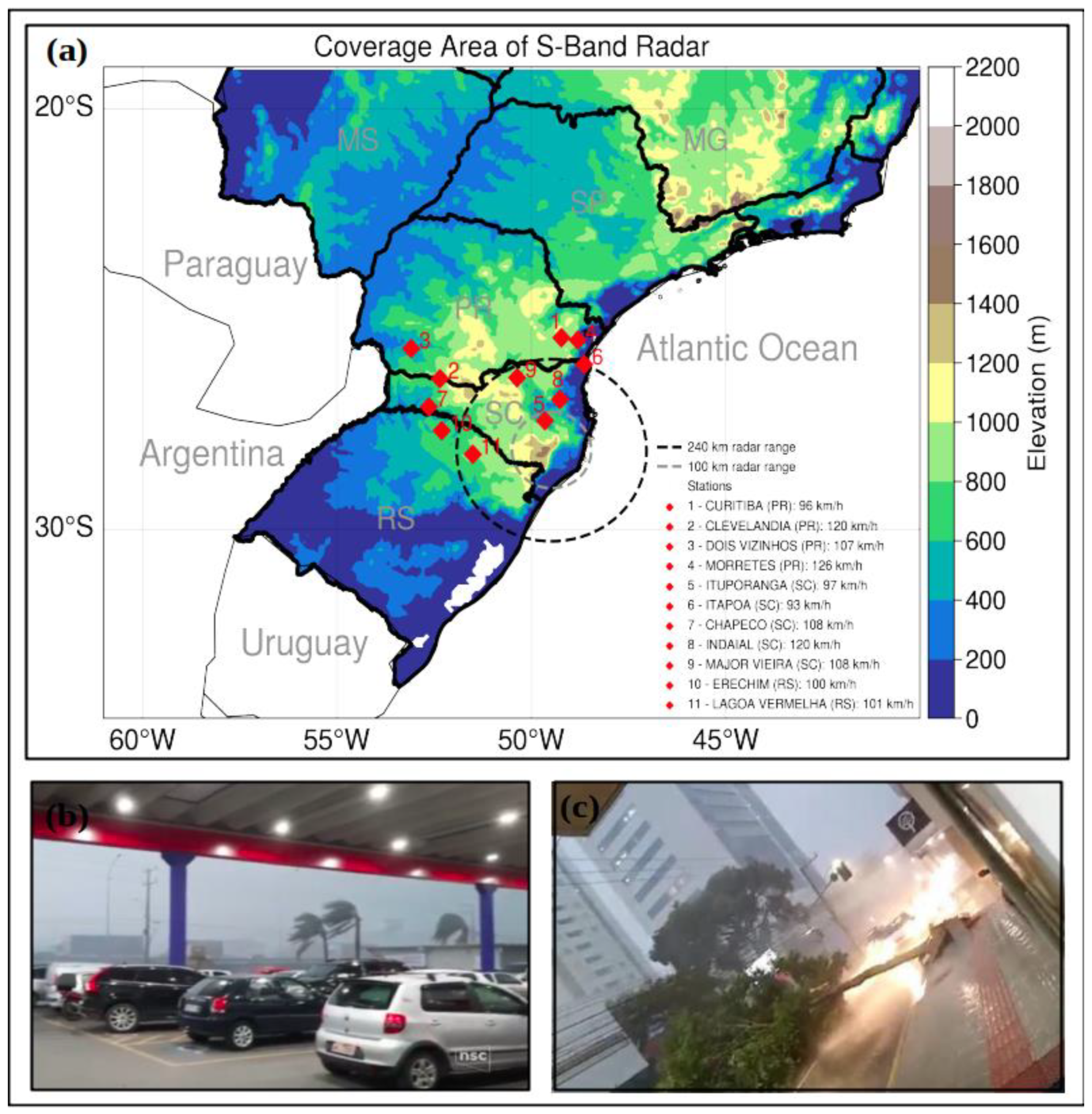
2.1. Region of Study

The studied region is composed of southern Brazil, mainly Santa Catarina (SC) state, and the southwestern South Atlantic Ocean (Figure 1a). Figure 1a also shows the Brazilian topography, the radar covered radius which is centered in Morro da Igreja (MI) in SC, and the meteorological stations from the Brazilian National Meteorological Institute (INMET), [71], with their wind intensity observation recording when the maximum wind associated to the squall line occurred.

2.2. Data

This study uses data from different sources as summarized in Table 1 and described below.

(a)

To describe the impacts of the squall line on the surface variables, hourly data of wind intensity and precipitation from INMET [71] automatic meteorological stations (Figure 1) were used;

(b)

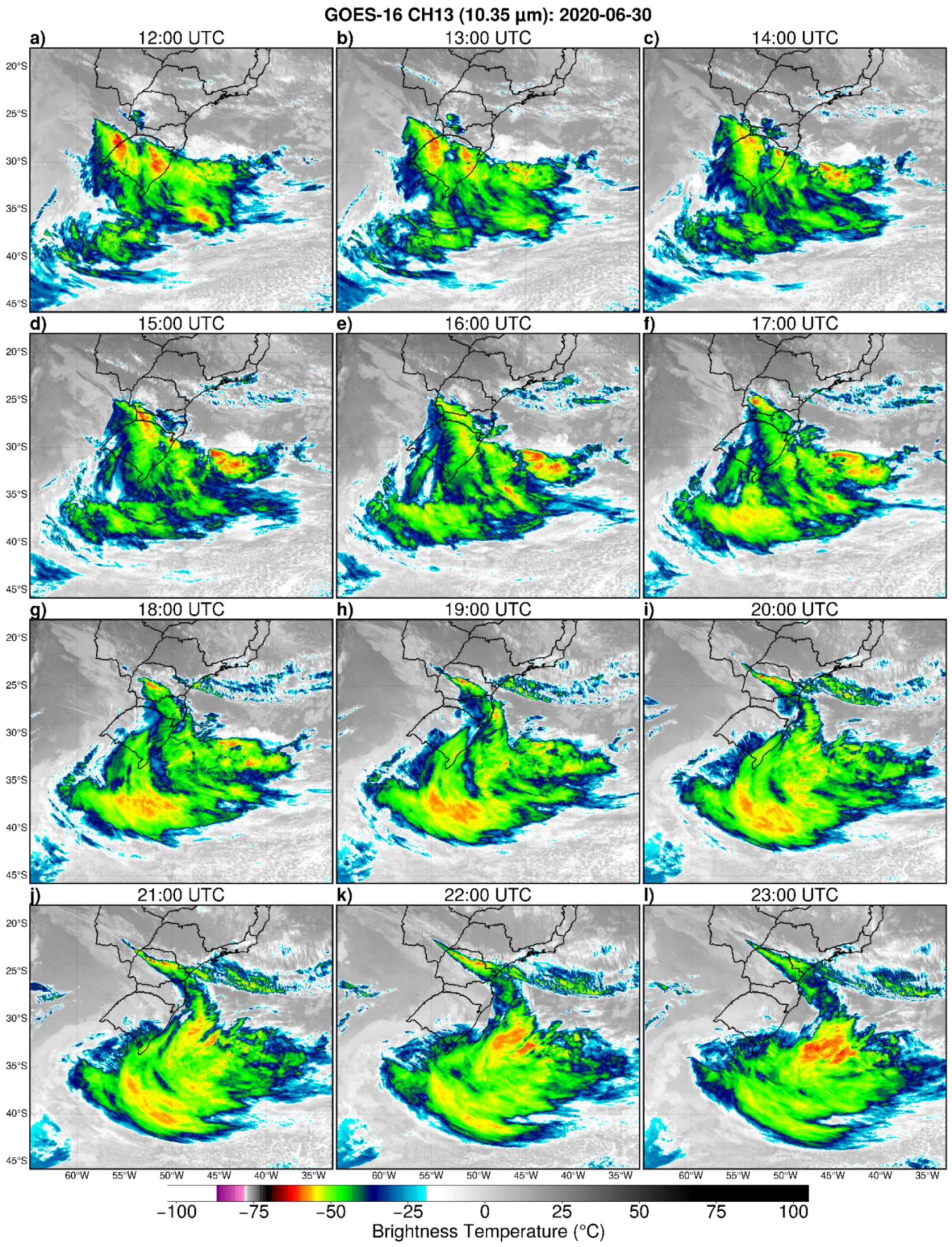
For the synoptic analysis, standard time data (0000, 0006, 1200, and 1800 UTC) of geopotential height, zonal and meridional wind components, temperature, relative humidity, mean sea level pressure, sea surface temperature, and latent and sensible heat fluxes from ERA5 reanalysis [72], provided by the European Center for Medium-Range Weather Forecasts were obtained. ERA5 was downloaded with 0.25° × 0.25° horizontal resolution for the period from 28 June to 3 July of 2020. For the generation of satellite images, brightness temperature data from the infrared channel 13 (IR, 10.30 µm) of the Geostationary Operational Environmental Satellite-16 (GOES-16) were used. These data belong to the National Oceanic and Atmospheric Administration (NOAA) with a spatial resolution of 2 km and a temporal resolution of 10 min [73]. The data are reprocessed by the Center for Climate Studies and Weather Forecasting (CPTEC) from National Institute for Space Research (INPE) and freely available (http://ftp.cptec.inpe.br/goes/goes16/retangular/ (accessed on 25 November 2022). Satellite data are applied in both the synoptic and mesoscale analyses of this study;

(c)

For the numerical experiments with Weather Research Model (WRF), initial and boundary conditions were obtained from the analysis of the Global Forecast System (GFS) of the National Center for Environmental Forecasting [74] and of ERA5 reanalysis [72];

(d)

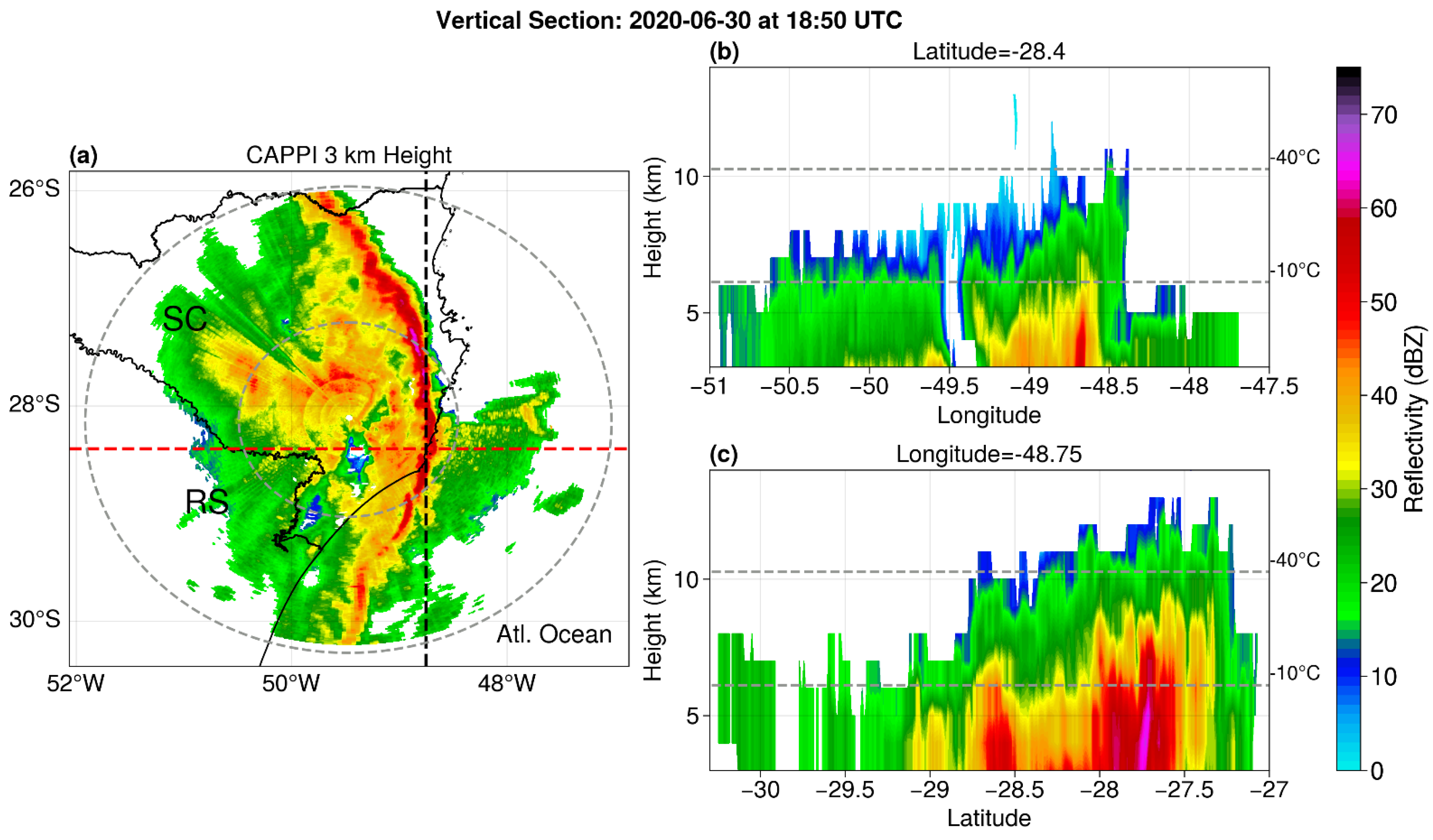
To estimate the physical properties of the squall line, reflectivity data from the Morro da Igreja radar were used. This weather radar operates in S-band radar (10 cm) frequency with temporal resolution of 10 min and 240 km distance range, and is located in the state of SC. The radar belongs to the Department of Airspace Control (DCEA) and is operated by the Aeronautics Command Meteorology Network [75]. A Constant Altitude Plan Position Indicator (CAPPI) with 1 km of vertical and horizontal resolution, from 3 to 15 km heights was produced;

(e)

The electrical activity of the squall line was evaluated using return stroke occurrence provided by the Brazilian Electrical Discharge Detection System—BrasilDAT [76,77] for 30 June 2020. This network is based on the technology of the Earth Network sensors and covers the south, southeast, midwest, and northeast regions of Brazil. It also employs the time-of-arrival method (TOA) and detects return flash emissions between 1 Hz and 12 MHz. The technology used by BrasilDAT allows discrimination between intracloud (IC) and cloud-to-ground (CG) return stroke, and the data are composed of the latitude, longitude, peak current, and other information of IC and CG return strokes. The total lightning was determined, which represents the sum of IC and CG lightning. This information was interpolated for a grid with 4 km spatial resolution. In addition, hourly accumulation of total lightning close to the region of the squall line was produced.

Table 1. Summary of the dataset used in the study.

Dataset	Horizontal Resolution	Frequency	Reference	Link to Access
ERA5	0.25° × 0.25°	Hourly	Herbach et al. (2020) [72]	https://cds.climate.copernicus.eu (accessed on 12 February 2022)
GFS	0.25° × 0.25°	Hourly	GFS [74]	https://www.nco.ncep.noaa.gov/ (accessed on 12 February 2022)
REDEMET	500 km (radius)	10 min	REDEMET [75]	https://www.redemet.aer.mil.br/ (accessed on 12 February 2022)
GOES-16	2 km	10 min	Minghelli et al. (2021) [73]	https://www.ngdc.noaa.gov/ (accessed on 22 November 2022)
BrasilDAT	Grid Point	nanoseconds	Naccarato and Machado (2019) [76]	http://www.inpe.br/webelat/ (accessed on 22 November 2022)
INMET	local	Hourly	INMET [71]	https://portal.inmet.gov.br/ (accessed on 12 February 2022)

Table 1. Summary of the dataset used in the study.

Dataset	Horizontal Resolution	Frequency	Reference	Link to Access
ERA5	0.25° × 0.25°	Hourly	Herbach et al. (2020) [72]	https://cds.climate.copernicus.eu (accessed on 12 February 2022)
GFS	0.25° × 0.25°	Hourly	GFS [74]	https://www.nco.ncep.noaa.gov/ (accessed on 12 February 2022)
REDEMET	500 km (radius)	10 min	REDEMET [75]	https://www.redemet.aer.mil.br/ (accessed on 12 February 2022)
GOES-16	2 km	10 min	Minghelli et al. (2021) [73]	https://www.ngdc.noaa.gov/ (accessed on 22 November 2022)
BrasilDAT	Grid Point	nanoseconds	Naccarato and Machado (2019) [76]	http://www.inpe.br/webelat/ (accessed on 22 November 2022)
INMET	local	Hourly	INMET [71]	https://portal.inmet.gov.br/ (accessed on 12 February 2022)

2.3. Synoptic Analysis

2.3.1. Cyclone Lifecycle

Cyclogenesis, the development of a near-surface cyclone, is defined when the first closed isobar (lines of the equal pressure values) appears in the mean sea level pressure (MSLP) field considering isobars displayed at 3 hPa. Cyclolysis is the decay of the system and it begins after the phase of maximum cyclone intensification or occlusion (maturity). In the occlusion phase, the near-surface cyclone is coupled with a wave at mid/high atmospheric levels and, if drawn, its relative vorticity will appear as a vertically extended tube connecting the near-surface cyclone with the center of the wave at mid-upper levels [78]. In this case study, the synoptic analysis will be performed from 24 h before the genesis (what will be called pre-cyclogenesis) until the initial phase of decay. For each time step of the cyclone (in this study, every 6 h), the lowest value of MSLP and its geographic coordinates (latitude, longitude) are registered. It allows the representation of the system’s trajectory and the MSLP time evolution.

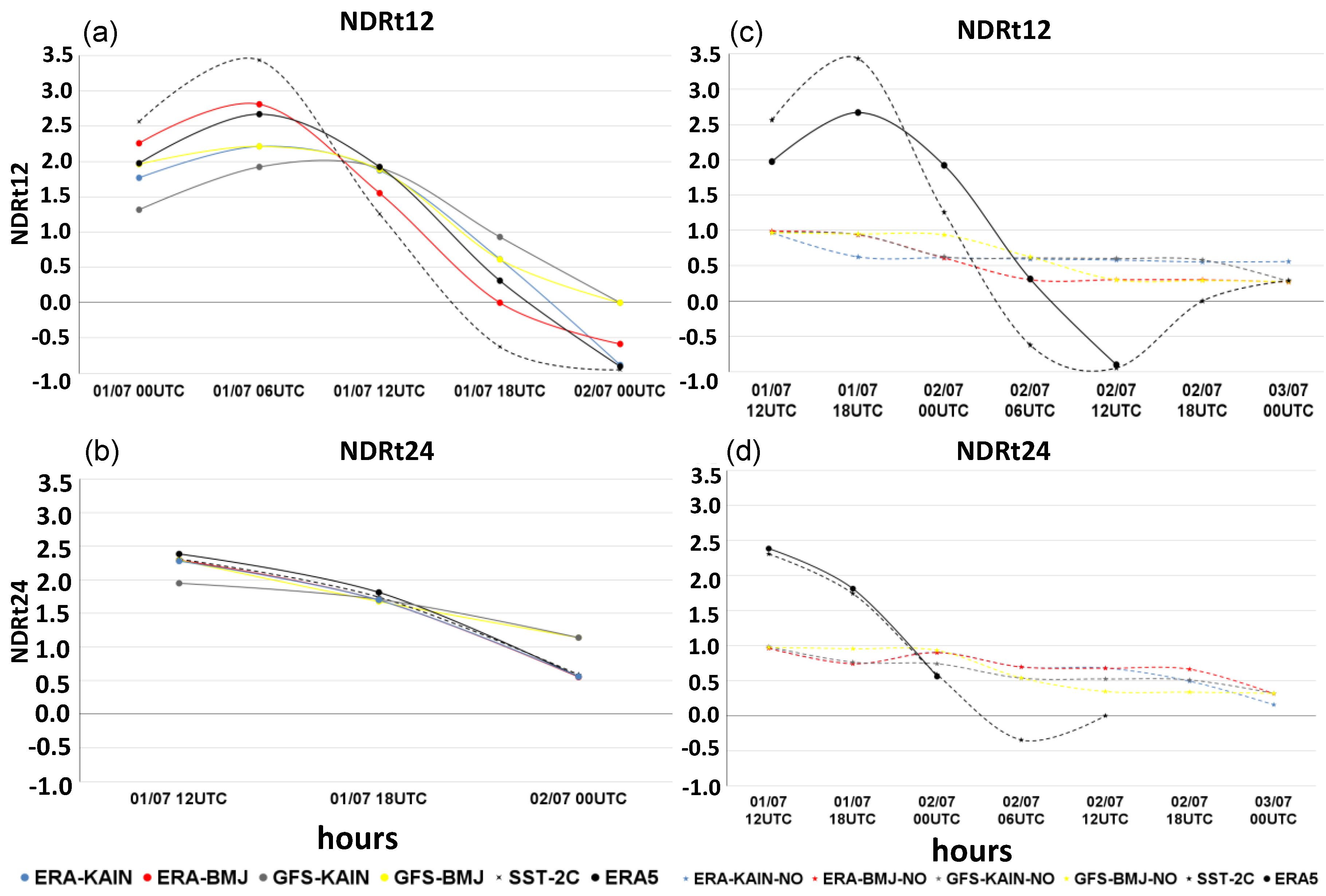
2.3.2. Explosive Cyclone

To classify the cyclone as an explosive system, two approaches can be applied: Sanders and Gyakum [1], hereafter SG, and Zhang et al. [2]. The difference between both is that SG [1] consider a period of 24 h to compute the Normalized Central Pressure Deepening Rate (NDR) and a latitude of 60° as the adjusted latitude in geostrophically equivalent rate for defining an explosive cyclone (Equation (1)). In contrast, Zhang et al. [2] use 12 h and a latitude of 45° (Equation (2)). The changes carried out by Zhang et al. [2] are justified because nowadays there is data with higher frequency than in the 1980s, and explosive cyclones are more frequently located at a latitude of 45°.

Here we exemplify the calculus of NDR considering the method by SG [1]. The first period of 24 h within the cyclone’s lifetime, i.e., fifth time step in the tracking, is considered. The change in pressure during this period is computed by subtracting the MSLP in the fifth time step (t₂₄) of the cyclone from the first cyclone time step (t₀). In the next iteration, the sixth and second time steps are subtracted, and so on. In both equations, we kept the sine factor with positive values and multiplied the NDR by −1 to obtain NDR > 1 for an explosive cyclone. Explosive cyclones can also be classified as weak (1.0 ≤ NDR < 1.3), moderate (1.3 ≤ NDR < 1.8), and strong (NDR ≥ 1.8) following Sanders [79] when NDR is calculated by Equation (1), and as weak (1.0 ≤ NDR < 1.3), moderate (1.3 ≤ NDR < 1.7), strong (1.7 ≤ NDR < 2.3), and super (NDR ≥ 2.3) when it is calculated by Equation (2). Note that Zhang et al.’s (2017) classification includes a class “super” because systems have been observed overtaking SG’s thresholds.

$$\mathrm{NDR}{\mathrm{t}}_{24}=-1 \frac{\left(MSLP t_{24}-MSLP t_0\right)}{24} \frac{sin 60°}{sin \left(\left|lat t_{24}\left|+\right|lat t_0\right|\right)/2} ,$$

(1)

$$\mathrm{NDR}{\mathrm{t}}_{12}=-1 \frac{\left(MSLP t_{12}-MSLP t_0\right)}{12} \frac{sin 45°}{sin \left(\left|lat t_{12}\left|+\right|lat t_0\right|\right)/2} ,$$

(2)

where NDR indicates the Normalized Central Pressure Deepening Rate and lat is the latitude of the cyclone center. The data used to calculate these equations were obtained with the cyclone’s tracking (Section 2.3.1).

2.3.3. Frontogenetic Function

To identify the regions with an intense horizontal gradient of temperature (𝛁T), the frontogenetic function (F) derived originally by Petterssen [80] and presented by Schultz et al. [35] was used. F is computed as

$$F =\frac{1}{2} |𝛁T|(E cos2\beta - D),$$

(3)

where 𝛽 is the local angle between the temperature and the axis of dilatation, D is the divergence of the horizontal wind component $\left(D=\frac{\delta u}{\delta x}+\frac{\delta v}{\delta y}\right),$ and E is deformation given by

$$E=(E_{\mathit{st}}^2 + E_{\mathit{sh}}^2) \frac{1}{2}.$$

(4)

E_st = $\frac{\delta u}{\delta x}-\frac{\delta v}{\delta y}$ is the stretching deformation and E_sh = $\frac{\delta v}{\delta x}+\frac{\delta u}{\delta y}$ is the shearing deformation. F is computed at 850 and 700 hPa and the average of these levels is calculated. Positive (negative) values of F indicate frontogenesis (frontolysis).

2.3.4. Atmospheric Fields

Based on the variables presented in Section 2.2, different atmospheric fields are drawn to describe the development of the cyclone: (a) MSLP (hPa), thickness between 500–1000 hPa and wind intensity higher than 30 m s⁻¹ at 250 hPa (which is indicative of jet streams); (b) geopotential height (mgp) at 250 hPa and vertical wind shear of the horizontal wind (250–850 hPa); (c) streamlines at 850 hPa and 250 hPa; (d) frontogenetic function at 850 hPa and equivalent potential temperature at 850 hPa. These fields are plotted for the main synoptic hours (0000, 0006, 1200, and 1800 UTC) between 0600 UTC on 30 June and 0000 UTC on 2 July 2020.

2.4. Physical Processes and Numerical Simulations

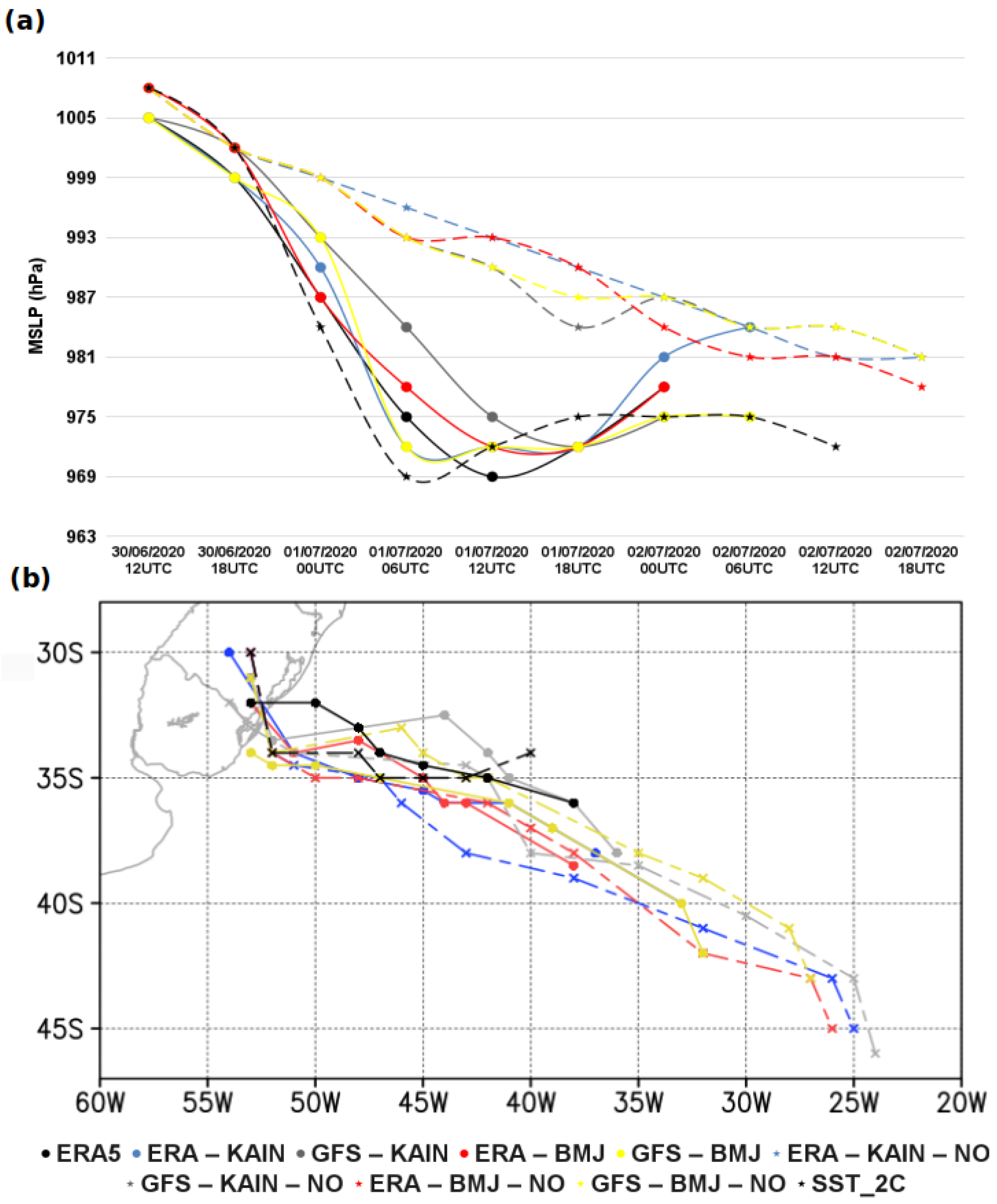
2.4.1. Model and Experiment Description

The Weather Research Forecast (WRF) model version 4.2.2 [81] is used for evaluating the influence of turbulent heat fluxes on the explosive characteristic of our case study. Nine experiments were carried out (

Table 2. Configuration of the experiments: nomenclature, boundary conditions, SST condition, cumulus parameterization scheme, and turbulent heat fluxes turn on or turn off.

Experiment	Boundary Conditions	SST	Cumulus Convection	Fluxes
ERA_KAIN	ERA	Normal	KF	ON
ERA_BMJ	ERA	Normal	BMJ	ON
GFS_KAIN	GFS	Normal	KF	ON
GFS_BMJ	GFS	Normal	BMJ	ON
ERA_KAIN_NO	ERA	Normal	KF	OFF
ERA_BMJ_NO	GFS	Normal	BMJ	OFF
GFS_KAIN_NO	GFS	Normal	KF	OFF
GFS_BMJ_NO	GFS	Normal	BMJ	OFF
SST_2C	ERA	+2 °C	BMJ	ON

) and the common features among them are that simulations were integrated with a horizontal resolution of 12 km and with 38 vertical levels in the region from 10° to 50° S and from 20° to 90° W; the physical parameterization schemes used are New Thompson microphysics for the microphysical processes [82], YSU for surface layer processes [83], Eta Similarity Scheme for land–surface interactions [84], Dudhia for shortwave radiation [85], and RRTM for longwave radiation [86]. As shown in Table 2, the sensitivity experiments include two cumulus convection schemes: Kain and Fritsch [87] and Betts Miller Janjic [88,89], and turbulent heat fluxes parameterization turned on or off in the model. For the experiments, we also evaluate two initial and boundary conditions: ERA5 reanalysis [72] and the analysis of GFS [74], both with a horizontal resolution of 0.25° and frequency of 6 h. Moreover, all experiments used the SST provided by these datasets. The simulations were performed for 96 h starting at 0000 UTC on 29 June 2020.

The first 24 h of the simulations were discarded to avoid numerical spin-up errors [82]. An additional experiment to study the impact of the sea–air interaction, where SST is warmed at 2 °C using the same configuration of the ERA_BMJ experiment (Table 2), was also carried out.

2.4.2. Sea–Air Interaction

One way to analyze the sea–air interaction is through the turbulent sensible (SH) and latent (LH) heat fluxes. Equations (5) and (6) show that the energy transfer in the interface sea–air occurs associated with vertical gradients of temperature (T_s − T_2m in Equation (5)), specific humidity (q_sst − q_2m in Equation (6)), and wind intensity near the surface (10 m height).

$$SH={\mathsf{\rho }}_{\mathrm{a}} {\mathrm{c}}_{\mathrm{p}} {\mathrm{C}}_{\mathrm{h}} {\mathrm{U}}_{10} ({\mathrm{T}}_{\mathrm{s}}-\mathrm{T}{2}_{\mathrm{m}}),$$

(5)

$$LH={\mathsf{\rho }}_{\mathrm{a}} {\mathrm{L}}_{\mathrm{e}} {\mathrm{C}}_{\mathrm{e}} {\mathrm{U}}_{10} ({\mathrm{q}}_{\mathrm{sst}}-\mathrm{q}{2}_{\mathrm{2m}}),$$

(6)

where ⍴_a is the air density (~1.2 kg m⁻³), c_p is the specific heat of dry air at constant pressure (1004 J K⁻¹ kg⁻¹), C_e and C_h are the turbulent exchange coefficients for latent and sensible heat, respectively, and their values are dependent of the stability conditions [90,91]; U₁₀ is the height at 10 m for the wind velocity, Le is the latent heat of vaporization (~2.26 × 10⁶ J kg⁻¹), T_s and T_2m are, respectively, sea surface temperature and air temperature at 2 m height, and q_sst and q_2m are, respectively, the saturation specific humidity at sea level and the specific humidity at 2 m height.

To obtain q_sst, it is necessary to calculate the saturation vapor pressure ($e$*) and for q_2m, the partial vapor pressure (e). According to [92], the equations are:

$$e* =6.112\exp \left(\frac{17.62 Tsst}{243.12+Tsst}\right),$$

(7)

$$e =6.112\exp \left(\frac{17.62 T2m}{243.12+T2m}\right),$$

(8)

where T_sst and T_2m are given in °C and $e$* and e in hPa.

From Equations (5) and (6), it is possible to obtain q_sst and q_2m [92,93]:

$${\mathrm{q}}_{\mathrm{sst}}=0.622\left(\frac{e*}{P}\right),$$

(9)

$$\mathrm{q}{2}_{\mathrm{m}}=0.622\left(\frac{e}{P}\right),$$

(10)

where $e$* is the saturation vapor pressure in g kg⁻¹ and P is the surface pressure (hPa).

Over the ocean, in general, turbulent heat fluxes add energy to the atmosphere. This energy is important to convection and latent heat release by condensation, which is a diabatic process. Hence, we analyze the total turbulent heat fluxes (latent heat + sensible heat) and 10 m wind intensity along the simulated cyclone. It is important to highlight that precipitation is a proxy for diabatic processes (the greater the volume of rain, the greater the latent heat released by condensation in clouds must be), then, this variable is also analyzed.

2.5. Severe Weather/Mesoscale Convective Systems

Satellite and radar images were analyzed to describe the mesoscale convective systems embedded in the cold front structure. From the satellite, the brightness temperature was displayed. This variable indicates the temperature at the top of the clouds, and white colors are an indication of deep convection. From the radar, the reflectivity (CAPPI 3 km) was shown to represent, in higher resolution, the growth/evolution and displacement of the squall line. Based on CAPPI, we show that the squall line is most intense at 1850 UTC on 30 June, hence, a vertical cross section was taken to analyze the depth and intensity of the clouds. Finally, the time with a higher frequency of total lightning (sum of IC and CG return stroke) was shown.

The scientific questions, methodology, and data of this study are summarized in Figure 2.

3. Results

3.1. Synoptic Analysis

3.1.1. Physical Processes of Cyclogenesis

Initially, MSLP, wind intensity at 250 hPa, and 500–1000 hPa thickness from ERA5 were plotted every 6 h from 0600 UTC 30 June 2020 to 0000 UTC 2 July 2020. The complete set of figures was analyzed, and those which were more representative of the cyclone lifecycle are presented in Figure 3. Cyclogenesis, indicated by an isobar of 1006 hPa, occurs at 1200 UTC on 30 June 2020 between southern Brazil, Uruguay, and the South Atlantic Ocean (Figure 3b). After its genesis, the cyclone moves to the southeast and reaches its maximum intensity (occlusion phase), with a central pressure of 969 hPa, at 1200 UTC on 1 July 2020 (Figure 3f). During the occlusion, the near-surface cyclone center is located southward of the polar jet at 250 hPa (Figure 3g). The period from 0000 UTC on 2 July 2020 will be considered as the decaying phase of the cyclone since the system tends to split into two low-pressure centers (Figure 3h).

The main physical process responsible for the cyclogenesis is a middle-upper trough traveling from the Pacific to the Atlantic Ocean, as indicated by the configuration of the upper-level winds and 500–1000 hPa thickness in Figure 3a,b, and by the geopotential height at 300 hPa in Figure 4a,b. The region downstream of the trough is characterized by wind divergence (Figure 4b,c), which helps to organize upward movements in the atmosphere and, consequently, to decrease MSLP. This physical process is the most common for cyclogenesis in the studied region [7,18,19,40,94,95].

3.1.2. Explosive Phase

Through the NDR_t12 (Zhang et al. [2]) and NDR_t24 (SG [1]) methodologies (Section 2.3.2), it is possible to verify that the cyclone reaches the explosive phase 12 h and 24 h, respectively, after cyclogenesis (

Table 3. Cyclone lifecycle: latitude, longitude, MSLP (hPa) at the cyclone center, and NDR every 6 h (UTC). NDR_t24 and NDR_t12 follow SG [1] and Zhang et al. [2], respectively. The dates of genesis, explosive phase, maturity, and decay are also indicated.

Date	Hour	Lat	Lon	MSLP	NDRt24	NDRt12
30/06 Genesis	1200	−32	−56	1006	-	-
30/06	1800	−30	−50	1000	-	-
01/07 Explosive	0000	−33	−47	988	-	1.9474 (strong)
01/07	0600	−34	−47	976	-	2.5966 (super)
01/07 Maturity	1200	−34	−45	969	2.3851 (strong)	1.9474 (strong)
01/07	1800	−35	−42	973	1.7888 (moderate)	0.3245
02/07 Decay	0000	−38	−35	979	0.5962	−0.9737

) since NDR_t12 = 1.9474 (strong) and NDR_t24 = 2.3851 (strong). Following Zhang et al.’s [2] methodology, the studied cyclone reaches the explosive phase before its 24 h. The same result is obtained when the SG methodology is adapted to 12 h (calculus not shown), which confirms fast pressure deepening. Figure 3d shows that the cyclone is over the ocean at the beginning of the explosive phase, and its central isobar is 988 hPa.

As the studied cyclone has explosive status, we also analyzed the background flow in order to classify it in one of the two conceptual models of cyclone development: Bjerknes and Solberg [41] or Shapiro and Keyser [34].

Figure 5 shows three time slices (cyclogenesis, beginning of the explosive phase, and maturity of the cyclone) considering different atmospheric variables: circulation at 250 and 850 hPa in order to identify diffluent and confluent flows; frontogenetic function and streamlines at 850 hPa, which allow the localization of the horizontal temperature gradients and possible frontal fracture; and equivalent potential temperature to help identify the frontal structures and compare them with extratropical cyclone conceptual models.

Considering the upper-level circulation, the cyclone develops under a region of diffluent flow at 250 hPa (bifurcation of the black lines in Figure 5a,b). At 850 hPa, the cyclone’s circulation is representative of the low-pressure system (Figure 5a,b). In the three snapshots (Figure 5d–f), the horizontal temperature gradients associated with the cold and warm fronts are well represented by the frontogenetic function, and the cold front is more extended (in the meridional direction) than the warm front (in the zonal direction). Moreover, there is no frontal fracture (which would be shown by blue colors in the frontogenetic function), and the cyclone is less zonally elongated than meridionally (Figure 5d–f). The spatial pattern of the equivalent potential temperature resembles the conceptual model of Bjerknes and Solberg with a sharp region of temperature gradient in the region of the occluded front (Figure 5g–i). Hence, it is different from Shapiro and Keyser’s model, which is characterized by an increase in the space between the isotherms and evolves to warm seclusion and a T-bone pattern (see Figure 5c,d from Reboita et al. [40], where the reader finds a case of Shapiro–Keyser cyclone for comparison with the present study). Due to the mentioned features, the studied cyclone follows the Bjerknes and Solberg model. Even not showing a warming seclusion, the cyclone acquires the status of explosive, which requires additional investigation. To address this issue, sensitivity experiments with the WRF model were performed and described in the next section.

3.2. Sensitivity Experiments

We begin this section by describing the time evolution of the central pressure of the cyclone and its trajectory in ERA5 and in the numerical experiments (Figure 6). All experiments simulated the cyclogenesis at the same time (1200 UTC 30 June 2020) and with similar MSLP patterns as shown in ERA5 (Figure 6a). This result is due to the fact that the cyclogenesis has a dynamic forcing (middle-upper level trough), as shown in Section 3.1.1, which is better simulated by models rather than thermodynamic forcing. In terms of the trajectory (Figure 6b), most of the experiments simulate the cyclone displacing southward when compared to ERA5. ERA_BMJ is the experiment in which the MSLP and the trajectory of the cyclone are closer to ERA5 during the first 36 h (

Table 4. Cyclone lifetime in the numerical experiments. In cyclolysis date, * indicates if the cyclone has association with another cyclone center, such as in ERA5.

Experiment	Cyclogenesis Date	Cyclolysis Date	Cyclogenesis Pressure (hPa)	Lifetime (Hours)	Traveled Distance (km)
ERA5	30/06 1200 UTC	02/07 0000 UTC	1005	36	1666
ERA_KAIN	30/06 1200 UTC	02/07 0600 UTC *	1005	40	1888
ERA_BMJ	30/06 1200 UTC	02/07 0000 UTC *	1005	36	1666
GFS_KAIN	30/06 1200 UTC	02/07 1200 UTC *	1005	36	2111
GFS_BMJ	30/06 1200 UTC	02/07 0600 UTC *	1005	40	2333
ERA_KAIN_NO	30/06 1200 UTC	02/07 1800 UTC	1008	52	3111
ERA_BMJ_NO	30/06 1200 UTC	02/07 1800 UTC	1008	52	2999
GFS_KAIN_NO	30/06 1200 UTC	02/07 1800 UTC	1008	52	3222
GFS_BMJ_NO	30/06 1200 UTC	02/07 1800 UTC	1008	52	2888
SST_2C	30/06 1200 UTC	02/07 1200 UTC	1008	46	1444

).

Although, in the experiments with the turbulent heat fluxes turned on, the use of different boundary conditions and cumulus convection schemes produces some differences in the central MSLP and trajectory of the cyclone when compared to ERA5, these differences can be considered not expressive. But it is not the case of the experiments with the turbulent heat fluxes turned off. The four experiments (ERA_KAIN_NO, ERA_BMJ_NO, GFS_KAIN_NO, and GFS_BMJ_NO) simulated a weaker cyclone six hours after the genesis, indicating that the turbulent heat fluxes and the associated diabatic processes are important to the deepening of the cyclone registered in ERA5. However, in these experiments, the simulated cyclone shows a longer lifetime because the cyclone tracking was not interrupted as in ERA5 when the cyclone splitted in two low-pressure centers. It is an additional evidence that the experiments without turbulent heat fluxes produce weaker near-surface systems.

As the turbulent heat fluxes are important for the development of the cyclone, we performed an additional experiment to verify the hypothesis if the cyclone becomes stronger considering a warmer SST of 2 °C. The main difference between this experiment and the others (Figure 6a) is the simulation of a deepening cyclone from 0000 to 1200 UTC on 1 July. In this experiment, the main cyclone is also spllited in two low-pressure centers, as seen in ERA5, and at this moment, we assume that cyclolysis occurred.

The NDR (SG and Zhang et al. [1,2]) for each numerical experiment is shown in Figure 7. NDR_t12 for all experiments with the turbulent heat fluxes on (ERA_KAIN, ERA_BMJ, GFS_KAIN, and GFS_BMJ) presents an explosive cyclone 12 h after the genesis (Figure 7a) and the NDR_t12 is higher in the numerical experiment with warmer SST (NDR_t12 = 3). Indeed, Figure 5a showed a more intense cyclone on 01 July in this experiment when compared with the others and ERA5. On the other hand, the experiments with the turbulent heat fluxes turned off do not simulate an explosive cyclone (Figure 7c), although the NDR_t12 is closer to one unit and keeps this feature throughout time. Considering NDR_t24 and the fluxes turned off, the values are also close to one unit. Even in the no flux experiments, the NDR is high (~1.0) because of the dynamical forcing (middle-upper trough; example in Figure 8a,b). However, the turbulent heat fluxes have an additional contribution to the pressure deepening of the studied cyclone pushing it to explosive status, and it is in line with others that documented a rapid cyclone deepening when comparing experiments with and without turbulent heat fluxes. One reason for this is that the turbulent heat fluxes provide heat and moisture to the atmosphere and it, consequently, contributes to the release of latent heat by condensation [40,96,97,98,99,100]. In other words, the turbulent heat fluxes warms the middle levels of the atmosphere, facilitating upward movement and leading to pressure deepening on the surface.

To discuss some differences between the experiments with the turbulent heat fluxes turned on and off, we selected a set of atmospheric fields of the experiments ERA_BMJ and ERA_BMJ_NO and present them in Figure 8. As previously mentioned, the middle-upper level forcing of the near-surface cyclone is similar in both experiments, which is shown through the jet streams, geopotential height, and mass divergence downstream of the trough at 250 hPa (Figure 8a–d). Although the geopotential height is similar between both experiments, differences appear when we compute ERA_BMJ_NO minus ERA_BMJ. Figure 8d shows the differences at the level of 250 hPa and indicates a predominance of negative values reaching −30 mgp mainly in the eastern sector of the trough. It means that the geopotential height is lower in the ERA_BMJ_NO, which is physically consistent. Since this experiment does not supply heat and moisture to the atmosphere, less diabatic heating occurs in the atmosphere column and, consequently, weaker warming and convection (upward movements) when compared to ERA_BMJ. Weaker vertical movements disturb less the upper levels leading to lower geopotential heigh.This result is supported by Figure 8g,h since in ERA_BMJ_NO weaker upward movements (variable W) occur in the warm sector of the cyclone (right side) in relation to ERA_BMJ.

All the mentioned features indicate that ERA_BMJ_NO simulates a weaker near-surface cyclone; another piece of evidence for this fact is the negative wind shear in the occluded region of the cyclone (Figure 8c,d). The southwestern sector of the cyclone in both experiments is characterized by negative vertical wind shear, indicating that the low-level circulation is more intense than at upper levels (Figure 8c,d). However, greater negative values in ERA_BMJ indicate more intense winds at low levels in this experiment.

The biggest difference between the experiments is in the 𝜃_e, a variable that compiles information on temperature and moisture (Figure 8e,f). ERA_BMJ simulates 𝜃_e with higher values indicating a warmer and wetter environment. In addition, there is a more intense horizontal gradient of 𝜃_e in the region of the cold front and from the cyclone center to its right side (Figure 8e,f). It is an important piece of evidence to the contribution of thermodynamic processes in the fast deepening of the cyclone. The cyclone warm sector is well evident in the cross section of 𝜃_e and the vertical velocity performed in the central latitude of the cyclone (Figure 8g,h). The more intense warming from the cyclone center to eastward in ERA_BMJ, as shown by the 𝜃_e vertical profile, is an indicator of the influence of the turbulent heat fluxes. These fluxes represent the sea–air interaction being responsible by an effective warming of the adjacent atmosphere, convection, and, consequently, latent heat release by condensation. A good proxy of this process chain is precipitation.

To evaluate the previous statement, Figure 9 shows the accumulated precipitation following the cyclone’s trajectory in three experiments: ERA_BMJ, ERA_BMJ_NO, and SST_2C. Comparing the first 12 h of the cyclone in the three experiments, the accumulated precipitation is greater in SST_2C followed by the ERA_BMJ and ERA_BMJ_NO. Therefore, it confirms the role of turbulent heat fluxes in the deepening of the cyclone. Figure 10 provides additional information about the physical processes associated with turbulent heat fluxes.

To finish this section, we also present some variables from Equations (5) and (6), i.e., total heat fluxes (latent plus sensible heat flux) and wind intensity at 10 m. In addition, accumulated precipitation is also shown. In the first 24 h of the cyclone’s lifecycle, near-surface winds are more intense in SST_2C followed by ERA_BMJ and ERA_BMJ_NO (Figure 10a). Intense winds are important to increase the vertical gradients of temperature and humidity, as described by Equations (5) and (6), and favor more intense exchanges in total heat fluxes (Figure 10b) from the sea to the air. We do not show this variable for ERA_BMJ_NO because it was turned off in the simulation. At the same time, when the total heat fluxes are higher, precipitation also reaches its peak (Figure 10c), highlighting the role of the diabatic processes and, consequently, the cyclone deepening. If we compare ERA_BMJ and SST_2C, the latter has more intense sea–air energy transfer (Figure 10b). It supports the idea that in the studied case warmer SST contributes to increase the sea–air exchanges and strengthens the near-surface cyclone via diabatic processes.

3.3. Mesoscale Analysis and Physical Properties of the Squall Line

Brightness temperature (T_b) measured by satellites means cloud top temperature. Lower values of T_b are one indicative of deeper clouds [101], which is a consequence of intense convection (but it needs to be evaluated with caution since this variable can also indicate high clouds such as cirrus). Hence, T_b can be used to identify precipitating systems such as cold and warm fronts associated with cyclones and, in some cases, pre-frontal squall lines. This later appears as a sharp border ahead of a cold front but, in general, its identification is not easy in satellite images [102].

To know the convective cloud cover distribution on the day of the registered damages in SC state (30 June 2020), T_b is shown in Figure 11. Clouds with T_b < −25 °C appear over the SC state at 1400 UTC. From this time, there is a northeast displacement of the clouds and, between 1500 and 1900 UTC, the state is covered by cold top clouds. From 1900 UTC, the continental area covered by clouds with T_b < −25 °C decreases since the cloud system displaces towards the ocean. The sequence of frames in Figure 11 does not allow us to distinguish the narrow cumulonimbus cloud band which is indicative of a squall line.

One way to obtain more details about the mesoscale convective systems and their cloud vertical structure is by using reflectivity from meteorological radar [103,104,105]. Figure 12 presents the radar reflectivity on 30 June 2020 and highlights a well-defined squall line moving from west to east over southern Brazil. This system has a better configuration between 1800 and 1900 UTC, and around 1820 and 1830 UTC the squall line meridionally extends crossing all SC states in its eastern sector (Figure 12f,g). Some studies suggest applying reflectivity thresholds to define convective precipitation occurrence [103,104,105]. For example, Zhang et al. [106] used two reflectivity criteria for convective precipitation: where the reflectivity had to be greater than 50 dBZ at any height and greater than 30 dBZ at −10 °C height or above. Rain intensity can be also classified through dBZ values. NOAA, in their website (https://www.weather.gov/jetstream/refl (accessed on 11 September 2022)), presents a table for this purpose. In addition, it is indicated that values from 60 to 65 dBZ are about the level where 2.5 cm diameter hail can occur. In all frames shown in Figure 12, the narrow line with red color presents values higher than 45 dBZ, which is indicative of convective rainfall and hail [101,107,108,109,110] and is a proxy to characterize a squall line. Hail occurrence is important to storm electrification [105,111,112,113].

Although a detailed description of the squall line genesis is beyond the scope of this study, we present some physical considerations about the development of pre-frontal squall lines based on the literature. According to Browning [60], pre-frontal squall lines occur in association with lines of deep convective cells that break out within warm sectors, often 200–300 km ahead of the surface cold front, in a cyclone wave. In other words, there is a northward flow (such as a low-level jet), which is ahead and parallel to the cold front, being forced to lift as it meets relatively cold air near the warm front. At the same time, in middle-upper levels, there is a dry flow from west to east (westerlies) over the warm flow that helps the air at low levels to become more unstable and to develop the squall line (for example, [114,115,116,117]). The low-level jet and the westerlies in our case study can be seen in Figure 4a,b and Figure 5a. In addition, the westerlies over SC are also shown in Figure 3b,c. However, this pattern is common in cyclones that develop near the southern Brazilian coast [7,19,94] and most of them do not appear associated with squall lines. Thus, a question that deserves attention in another study is the description of the additional physical drivers that lead to squall line organization. We have an initial hypothesis that the vertical wind shear is mainly responsible for squall line development [118], which is supported by the literature [119,120,121,122,123,124,125].

Squall lines are responsible for severe weather, such as intense rainfall and strong winds [126,127,128,129,130]. Figure 13 shows hourly precipitation and wind gusts registered in some meteorological stations indicated in Figure 1. In the three states (Paraná, Santa Catarina, and Rio Grande do Sul), precipitation and winds were more intense between 1600 and 2000 UTC on 30 June 2020. Wind gusts overtake 93 km h⁻¹ (a threshold for severe thunderstorms) in Ituporanga, Indaial, and Major Vieira weather stations in SC (Figure 13e). At 1850 UTC, the squall line showed great values of reflectivity and crossed the SC state. Hence, we performed an analysis of the internal structure of the squall line using radar imagery. Analyzing two vertical cross sections of the squall line (Figure 14), we can see that the depth of the storm overtakes 10 km in height while the reflectivity above 50 dBZ occurs below this altitude and near 28.0–27.5° S. Storms with great vertical extension and reflectivity higher than 40–45 dBZ are associated with graupel and hail formation [108,109]; these hydrometeors are important for storm electrification and, consequently, electrical discharges [131]. The lightning is formed through the collision of ice crystals, graupel, and hail in the ascendent currents inside the storm clouds. During the collision of these hydrometeors, the separation of electrical charges and an increase in the electric field in the clouds occur, which lead to the potential to break the dielectric strength of the air and, consequently, to the electrical discharge.

Total lightning occurrences are shown in Figure 15, which is the sum of all lightning strokes that occurred on 30 June, totaling 418,145 occurrences on that day (Figure 15a). The evolution of the total lightning in one hour is presented in Figure 15b, where it is possible to observe the local and time of the lightning in SC (from 4:30 p.m. to 7:30 p.m. local time), after the formation of a squall line in the east of the state of SC (Figure 14).

4. Conclusions

On 30 June 2020, SC state in southern Brazil was greatly affected by precipitation and strong winds that led to structural damages and the death of at least eleven people. The media attributed the damage to an explosive cyclone. Meteorologically speaking, it is wrong since the cyclone kept over the ocean and the cold front associated to this system that was the precursor of the favorable environment for the squall line development, which, consequently, was responsible for the severe weather. Since this event in 2020, people have become afraid of the word cyclone. Then, in this study, we provided a synoptic and numerical analysis of the extratropical cyclone and a discussion of some cloud physical properties of the squall line.

The studied cyclone had its genesis following the classical mechanism of development in the southern Brazil and Uruguay regions, which is the influence of a trough at mid-upper levels of the atmosphere that displaces from the South Pacific to the South Atlantic Ocean. The cyclone’s lifecycle followed the conceptual model of cyclone development of Bjerknes and Solberg, which is an indicative that the cyclone cannot develop a well-defined region of warm seclusion. The literature shows, in general, that warm seclusion is important to the rapid deepening of extratropical cyclones. However, in the studied case, even without a well-defined area of warm seclusion, the system evolved into an explosive system 12 h after the cyclogenesis.

A comparison between the sensitivity numerical experiments, considering the sensible and latent turbulent heat fluxes turned on and off in the WRF model, showed that the sea–air interaction (turbulent heat fluxes) contributed to the deepening of the cyclone leading it to the status of explosive since the no flux experiments simulated a weaker cyclone. Turbulent heat fluxes represent the transfer of heat and humidity from the sea to the atmosphere and, during the condensation processes at the middle levels, there is latent heat release, which warms the atmosphere and helps to decrease near-surface pressure. Therefore, these processes linked to the influence of the migratory trough at mid-upper levels of the atmosphere are responsible for the explosive feature of the studied cyclone.

The cyclonic wave with its cold front was responsible for creating an adequate environment for the development of a pre-frontal squall line. Our study did not have the intention of describing squall line genesis, but we suggest a detailed investigation of the vertical wind shear ahead of the cold front to understand the genesis of this system.

While satellite images do not clearly show the squall line ahead of the cold front, radar reflectivity data indicate the propagation of the squall line that reached the SC state. On 30 June 2020, the clouds in the squall line had more than 10 km of vertical extension and reflectivity higher than 40 dBZ in some parts of the storm, which is an indicator of hail and, consequently, is a required condition for storm electrification.

The analyses presented are important to add knowledge to explosive cyclone development near southern Brazil and to help weather forecasters in operational analysis. Even though the study is subject to limitations such as the physical parameterizations used in the model, it was able to describe the characteristics associated with the genesis and development of the cyclone. Finally, we would like to highlight that the present study enables further analysis to be completed, for instance, focusing on the frontal structure and squall line.

References

1. Sanders, F.; Gyakum, J.R. Synoptic-dynamic climatology of the “bomb”. Mon. Weather Rev. 1980, 108, 1589–1606. [Google Scholar] [CrossRef]
2. Zhang, S.; Fu, G.; Lu, C.; Liu, J. Characteristics of explosive cyclones over the Northern Pacific. J. Appl. Meteorol. Climatol. 2017, 56, 3187–3210. [Google Scholar] [CrossRef]
3. NDMAIS. Ventos Durante o Cyclone Bomba em Santa Catarina Chegaram a 168 km/h Aponta Epagri. 2020. Available online: https://ndmais.com.br/tempo/velocidade-durante-o-ciclone-bomba-em-santa-catarina-chegou-a-168-km-h-aponta-epagri/ (accessed on 14 January 2022).
4. Faria, L.F.; Reboita, M.S. Eventos Meteorológicos Associados ao Ciclone Explosivo Ocorrido em Junho de 2020 e Impactos Socioambientais no Estado de Santa Catarina. Geografia 2023, 48, 1–27. Available online: https://www.periodicos.rc.biblioteca.unesp.br/index.php/ageteo/article/view/16661/12645 (accessed on 24 February 2023).
5. GZH. Jornal Digital Gaúcho. 2020. Available online: https://gauchazh.clicrbs.com.br/ambiente/noticia/2020/07/ (accessed on 23 February 2022).
6. Gan, M.A.; Rao, V.B. Surface cyclogenesis over South America. Mon. Weather Rev. 1991, 119, 1293–1302. [Google Scholar] [CrossRef]
7. Seluchi, M.E. Diagnóstico y pronóstico de situaciones sinópticas conducentes a ciclogénesis sobre el este de Sudamérica. Geofísica Int. 1995, 34, 171–186. Available online: http://132.248.182.214/index.php/RGI/article/view/737 (accessed on 23 February 2022).
8. Hoskins, B.J.; Hodges, K.I. A new perspective on Southern Hemisphere storm tracks. J. Clim. 2005, 18, 4108–4129. [Google Scholar] [CrossRef]
9. Reboita, M.S.; Da Rocha, R.P.; Ambrizzi, T.; Sugahara, S. South Atlantic Ocean cyclogenesis climatology simulated by regional climate model (RegCM3). Clim. Dyn. 2010, 35, 1331–1347. [Google Scholar] [CrossRef]
10. De Jesus, E.M.; da Rocha, R.P.; Crespo, N.M.; Reboita, M.S.; Gozzo, L.F. Multi-model climate projections of the main cyclogenesis hot-spots and associated winds over the eastern coast of South America. Clim. Dyn. 2021, 56, 537–557. [Google Scholar] [CrossRef]
11. Lim, E.P.; Simmonds, I. Explosive cyclone development in the Southern Hemisphere and a comparison with Northern Hemisphere events. Mon. Weather Rev. 2002, 130, 2188–2209. [Google Scholar] [CrossRef]
12. Bluestein, H.B. Synoptic-Dynamic Meteorology in Midlatitudes: Observations and Theory of Weather Systems; Oxford University Press: New York, NY, USA, 1992; Volume 2. [Google Scholar]
13. Andrade, H.N.; Nunes, A.B.; Teixeira, M.S. South Atlantic explosive cyclones in 2014–2015: Study employing NCEP2 and MERRA-2 reanalyses. An. Acad. Bras. Ciências. 2022, 94. [Google Scholar] [CrossRef]
14. Avila, V.D.; Nunes, A.B.; Alves, R.C.M. Análise de um Caso de Ciclogênese Explosiva Ocorrido em 03/01/2014 no Sul do Oceano Atlântico. Rev. Bras. Geogr. Fís. 2016, 9, 1088–1099. [Google Scholar] [CrossRef]
15. Necco, G.V. Comportamiento de Vortices Ciclonicos En El Area Sudamerica Durante El FGGE: Ciclogenegis. Meteorologica 1982, 13, 7–19. [Google Scholar]
16. Necco, G.V. Comportamiento de Vortices Ciclonicos En El Area Sudamerica Durante El FGGE: Trayectorias y Desarrollos. Meteorologica 1982, 13, 21–34. [Google Scholar]
17. Sinclair, M.R. Objective identification of cyclones and their circulation intensity, and climatology. Weather Forecast. 1997, 12, 595–612. [Google Scholar] [CrossRef]
18. Vera, C.S.; Vigliarolo, P.K.; Berebery, E. Cold Season Synoptic-Scale Waves over Subtropical South America. Mon. Weather Rev. 2002, 130, 684–699. [Google Scholar] [CrossRef]
19. Reboita, M.S.; Da Rocha, R.P.; Ambrizzi, T. Dynamic and Climatological Features of Cyclonic Developments over Southwestern South Atlantic Ocean; Veress, B., Szigethy, P., Eds.; Horizons in Earth Science Research; Nova Science Publishers: Hauppauge, Germany, 2012; pp. 135–160. [Google Scholar]
20. Crespo, N.M.; da Rocha, R.P.; Sprenger, M.; Wernli, H. A potential vorticity perspective on cyclogenesis over centre-eastern South America. Int. J. Climatol. 2021, 41, 663–678. [Google Scholar] [CrossRef]
21. Crespo, N.M.; Reboita, M.S.; Gozzo, L.F.; de Jesus, E.M.; Torres-Alavez, J.A.; Lagos-Zúñiga, M.Á.; da Rocha, R.P. Assessment of the RegCM4-CORDEX-CORE performance in simulating cyclones affecting the western coast of South America. Clim. Dyn. 2022, 1–19. [Google Scholar] [CrossRef]
22. Reboita, M.S.; Reale, M.; da Rocha, R.P.; Giorgi, F. Future changes in the wintertime cyclonic activity over the CORDEX-CORE southern hemisphere domains in a multi-model approach. Clim. Dyn. 2021, 57, 1533–1549. [Google Scholar] [CrossRef]
23. Reboita, M.S.; Crespo, N.M.; Torres, J.A.; Reale, M.; Porfírio da Rocha, R.; Giorgi, F.; Coppola, E. Future changes in winter explosive cyclones over the Southern Hemisphere domains from the CORDEX-CORE ensemble. Clim. Dyn. 2021, 57, 3303–3322. [Google Scholar] [CrossRef]
24. Bitencourt, D.P.; Fuentes, M.V.; Cardoso, C.D.S. Climatology of explosive cyclones over cyclogenetic area of South America. Rev. Bras. Meteorol. 2013, 28, 43–56. [Google Scholar] [CrossRef]
25. Fink, A.H.; Pohle, S.; Pinto, J.G.; Knippertz, P. Diagnosing the influence of diabatic processes on the explosive deepening of extratropical cyclones. Geophys. Res. Lett. 2012, 39. [Google Scholar] [CrossRef]
26. Gozzo, L.F.; Rocha, R.P.D. Air–sea interaction processes influencing the development of a Shapiro–Keyser type cyclone over the subtropical South Atlantic Ocean. Pure Appl. Geophys. 2013, 170, 917–934. [Google Scholar] [CrossRef]
27. Willison, J.; Robinson, W.A.; Lackmann, G.M. The importance of resolving mesoscale latent heating in the North Atlantic storm track. J. Atmos. Sci. 2013, 70, 2234–2250. [Google Scholar] [CrossRef]
28. Neiman, P.J.; Shapiro, M.A. The life cycle of an extratropical marine cyclone. Part I: Frontal-cyclone evolution and thermodynamic air-sea interaction. Mon. Weather Rev. 1993, 121, 2153–2176. [Google Scholar] [CrossRef]
29. Zhang, Y.; Held, I.M. A linear stochastic model of a GCM’s midlatitude storm tracks. J. Atmos. Sci. 1999, 56, 3416–3435. [Google Scholar] [CrossRef]
30. Kouroutzoglou, J.; Flocas, H.A.; Hatzaki, M.; Keay, K.; Simmonds, I.; Mavroudis, A. On the dynamics of a case study of explosive cyclogenesis in the Mediterranean. Meteorol. Atmos. Phys. 2015, 127, 49–73. [Google Scholar] [CrossRef]
31. Piva, E.; Gan, M.A.; Moscati, M.C.L. The role of latent and sensible heat fluxes in an explosive cyclogenesis over South America. J. Meteorol. Soc. Jpn. 2011, 89, 637–663. [Google Scholar] [CrossRef]
32. Kang, J.M.; Son, S.W. Development Processes of the Explosive Cyclones over the Northwest Pacific: Potential Vorticity Tendency Inversion. J. Atmos. Sci. 2021, 78, 1913–1930. [Google Scholar] [CrossRef]
33. Seluchi, M.E.; Saulo, A.C. Possible mechanisms yielding an explosive coastal cyclogenesis over South America: Experiments using a limited area model. Aust. Meteorol. Mag. 1998, 47, 309–320. [Google Scholar]
34. Shapiro, M.A.; Keyser, D. Fronts, jet streams and the tropopause. In Extratropical Cyclones; American Meteorological Society: Boston, MA, USA, 1990; pp. 167–191. [Google Scholar] [CrossRef]
35. Schultz, D.M.; Keyser, D.; Bosart, L.F. The effect of large-scale flow on low-level frontal structure and evolution in midlatitude cyclones. Mon. Weather Rev. 1998, 126, 1767–1791. [Google Scholar] [CrossRef]
36. Reboita, M.S.; Gan, M.A.; Rocha RP, D.; Custódio, I.S. Ciclones em superfície nas latitudes austrais: Parte I-revisão bibliográfica. Rev. Bras. Meteorol. 2017, 32, 171–186. [Google Scholar] [CrossRef]
37. Grønås, S. The seclusion intensification of the New Year’s day storm 1992. Tellus A 1995, 47, 733–746. [Google Scholar] [CrossRef]
38. Brâncuş, M.; Schultz, D.M.; Antonescu, B.; Dearden, C.; Ştefan, S. Origin of strong winds in an explosive mediterranean extratropical cyclone. Mon. Weather Rev. 2019, 147, 3649–3671. [Google Scholar] [CrossRef]
39. Cordeira, J.M.; Bosart, L.F. Cyclone interactions and evolutions during the “Perfect Storms” of late October and early November 1991. Mon. Weather Rev. 2011, 139, 1683–1707. [Google Scholar] [CrossRef]
40. Reboita, M.S.; Gozzo, L.F.; Crespo, N.M.; Custodio, M.D.S.; Lucyrio, V.; de Jesus, E.M.; da Rocha, R.P. From a Shapiro–Keyser extratropical cyclone to the subtropical cyclone Raoni: An unusual winter synoptic situation over the South Atlantic Ocean. Q. J. R. Meteorol. Soc. 2022, 148, 2991–3009. [Google Scholar] [CrossRef]
41. Bjerknes, J.; Solberg, H. Life cycle of cyclones and the polar front theory of atmospheric circulation. Geofys. Publ. 1922, 3, 3–18. [Google Scholar]
42. Salio, P.; Nicolini, M.; Zipser, E.J. Mesoscale convective systems over southeastern South America and their relationship with the South American low-level jet. Mon. Weather Rev. 2007, 135, 1290–1309. [Google Scholar] [CrossRef]
43. Yang, Q.; Houze, R.A., Jr.; Leung, L.R.; Feng, Z. Environments of long-lived mesoscale convective systems over the central United States in convection permitting climate simulations. J. Geophys. Res. Atmos. 2017, 122, 13–288. [Google Scholar] [CrossRef]
44. Feng, Z.; Houze, R.A., Jr.; Leung, L.R.; Song, F.; Hardin, J.C.; Wang, J.; Homeyer, C.R. Spatiotemporal characteristics and large-scale environments of mesoscale convective systems east of the Rocky Mountains. J. Clim. 2019, 32, 7303–7328. [Google Scholar] [CrossRef]
45. Schumacher, R.S.; Rasmussen, K.L. The formation, character and changing nature of mesoscale convective systems. Nat. Rev. Earth Environ. 2020, 1, 300–314. Available online: https://www.nature.com/articles/s43017-020-0057-7 (accessed on 23 February 2023). [CrossRef]
46. Li, J.; Feng, Z.; Qian, Y.; Leung, L.R. A high-resolution unified observational data product of mesoscale convective systems and isolated deep convection in the United States for 2004–2017. Earth Syst. Sci. Data 2021, 13, 827–856. [Google Scholar] [CrossRef]
47. Lin, Y.L. Mesoscale Instabilities. In Mesoscale Dynamics Cambridge; Cambridge University Press: Cambridge, UK, 2007; pp. 229–271. [Google Scholar] [CrossRef]
48. Lima, K.B.; Aquino, F.E.; Moraes, D.S.; Palhoça, S.C. Impactos gerados por dois Complexos Convectivos de Mesoescala de diferentes extensões no sul do Brasil. Rev. Gestão Sustentabilidade Ambient. 2018, 7, 186–205. Available online: http://hdl.handle.net/10183/223089 (accessed on 23 February 2023). [CrossRef]
49. Moraes, F.D.; Aquino, F.E.; Mote, T.L.; Durkee, J.D.; Mattingly, K.S. Atmospheric characteristics favorable for the development of mesoscale convective complexes in southern Brazil. Clim. Res. 2020, 80, 43–58. [Google Scholar] [CrossRef]
50. McNulty, R.P. Severe and Convective Weather: A Central Region Forecasting Challenge. Weather Forecast. 1995, 10, 187–202. [Google Scholar] [CrossRef]
51. Bluestein, H.B.; Jain, M.H. Formation of mesoscale lines of precipitation: Severe squall lines in Oklahoma during the spring. J. Atmos. Sci. 1985, 42, 1711–1732. [Google Scholar] [CrossRef]
52. Lemon, L.R.; Doswell, I.I.I. CA Severe thunderstorm evolution and mesocyclone structure as related to tornadogenesis. Mon. Weather Rev. 1979, 107, 1184–1197. [Google Scholar] [CrossRef]
53. Silva Dias, M.A.F. Mesoscale systems and short-term weather forecasting. Rev. Bras. Meteorol. 1987, 2, 133–150. [Google Scholar]
54. Ribeiro, B.Z.; Seluchi, M.E. A climatology of quasi-linear convective systems and associated synoptic-scale environments in southern Brazil. Int. J. Climatol. 2019, 39, 857–877. [Google Scholar] [CrossRef]
55. Dorneles, V.R.; Riquetti, N.B.; Nunes, A. Forçantes dinâmicas e térmicas associadas a um caso de precipitação intensa sobre o Rio Grande do Sul, Brasil. Rev. Bras. Climatol. 2020, 26. [Google Scholar] [CrossRef]
56. Thompson, R.L.; Edwards, R.; Hart, J.A.; Elmore, K.L.; Markowski, P. Close proximity soundings within supercell environments obtained from the Rapid Update Cycle. Weather Forecast. 2003, 18, 1243–1261. [Google Scholar] [CrossRef]
57. Dupilka, M.L.; Reuter, G.W. Forecasting tornadic thunderstorm potential in Alberta using environmental sounding data. Part I: Wind shear and buoyancy. Weather Forecast. 2006, 21, 325–335. [Google Scholar] [CrossRef]
58. Kolendowicz, L.; Taszarek, M.; Czernecki, B. Atmospheric circulation and sounding-derived parameters associated with thunderstorm occurrence in Central Europe. Atmos. Res. 2017, 191, 101–114. [Google Scholar] [CrossRef]
59. Houze, R.A.; Smull, B.F.; Dodge, P. Mesoscale organization of springtime rainstorms in Oklahoma. Mon. Weather Rev. 1990, 118, 613–654. [Google Scholar] [CrossRef]
60. Browning, K.A. Conceptual models of precipitation systems. Weather Forecast. 1986, 1, 23–41. [Google Scholar] [CrossRef]
61. Schemm, S.; Wernli, H. The linkage between the warm and the cold conveyor belts in an idealized extratropical cyclone. J. Atmos. Sci. 2014, 71, 1443–1459. [Google Scholar] [CrossRef]
62. Cotton, W.R.; Anthes, R.A. Storm and Cloud Dynamics; Elsevier: Amsterdam, The Netherlands, 2013; Volume 44. [Google Scholar]
63. Neu, U.; Akperov, M.G.; Bellenbaum, N.; Benestad, R.; Blender, R.; Caballero, R.; Wernli, H. IMILAST: A community effort to intercompare extratropical cyclone detection and tracking algorithms. Bull. Am. Meteorol. Soc. 2013, 94, 529–547. [Google Scholar] [CrossRef]
64. Liberato, M.L.R.; Pinto, J.G.; Trigo, R.M.; Ludwig, P.; Ordóñez, P.; Yuen, D.; Trigo, I.F. Explosive development of winter storm Xynthia over the subtropical North Atlantic Ocean. Nat. Hazards Earth Syst. Sci. 2013, 13, 2239–2251. [Google Scholar] [CrossRef]
65. Pinto, R.; Martins, F.C. The Portuguese national strategy for integrated coastal zone management as a spatial planning instrument to climate change adaptation in the Minho River Estuary (Portugal NW-Coastal Zone). Environ. Sci. Policy 2013, 33, 76–96. [Google Scholar] [CrossRef]
66. Gaztelumendi, S.; Egaña, J.; Gelpi, I.R.; Carreño, S.; Gonzalez, M.; Liria, P.; Aranda, J.A. Characterization of coastal-maritime severe events in Basque Country. In Proceedings of the 7th EuroGOOS Conference, Lisboa, Portugal, 28–30 October 2014; Volume 2830. [Google Scholar]
67. Gaztelumendi, S.; Egaña, J.; Gelpi, I.R.; Carreño, S.; González, M.; Liria, P.; Esnaola, G.; Rubio, A.; Aranda, J.A. Analysis of Coastal-Maritime Adverse Events in Basque Country. In Proceedings of the 14th EMS 10th ECAC, Prague, Czech Republic, 6–10 October 2014; Available online: https://presentations.copernicus.org/EMS2014-450_presentation.pdf (accessed on 23 February 2023).
68. Reale, M.; Liberato, M.L.; Lionello, P.; Pinto, J.G.; Salon, S.; Ulbrich, S. A global climatology of explosive cyclones using a multi-tracking approach. Tellus A Dyn. Meteorol. Oceanogr. 2019, 71, 1611340. [Google Scholar] [CrossRef]
69. Allen, J.T.; Pezza, A.B.; Black, M.T. Explosive cyclogenesis: A global climatology comparing multiple reanalyses. J. Clim. 2010, 23, 6468–6484. [Google Scholar] [CrossRef]
70. Kuwano-Yoshida, A.; Enomoto, T. Predictability of explosive cyclogenesis over the northwestern Pacific region using ensemble reanalysis. Mon. Weather Rev. 2013, 141, 3769–3785. [Google Scholar] [CrossRef]
71. Instituto Nacional De Meteorologia (INMET). Dados Meteorológicos. Banco de Dados Meteorológicos. 2022. Available online: https://bdmep.inmet.gov.br/ (accessed on 2 March 2022).
72. Hersbach, H.; Bell, B.; Berrisford, P.; Biavati, G.; Dee, D.; Horányi, A.; Nicolas, J.; Peubey, C.; Radu, R.; Rozum, I.; et al. The ERA5 Global Atmospheric Reanalysis at ECMWF as a comprehensive dataset for climate data homogenization, climate variability, trends and extremes. Geophys. Res. Abstr. 2019, 21. Available online: https://ui.adsabs.harvard.edu/abs/2019EGUGA..2110826H/abstract (accessed on 23 February 2023).
73. Minghelli, A.; Chevalier, C.; Descloitres, J.; Berline, L.; Blanc, P.; Chami, M. Synergy between Low Earth Orbit (LEO)—MODIS and Geostationary Earth Orbit (GEO)—GOES Sensors for Sargassum Monitoring in the Atlantic Ocean. Remote Sens. 2021, 13, 1444. [Google Scholar] [CrossRef]
74. Global Forecast System—GFS. Available online: https://www.ncei.noaa.gov/products/weather-climate-models/global-forecast (accessed on 10 January 2022).
75. Redemet. Brazilian Air Force. Brazil. Available online: https://www.redemet.aer.mil.br/ (accessed on 3 July 2020).
76. Naccarato, K.; Machado, L. Brazil BrasilDAT Lightning Network Data. Version 1.0. UCAR/NCAR—Earth Observing Laboratory. 2019. Available online: https://doi.org/10.26023/N9QW-SAKN-R311 (accessed on 23 December 2022).
77. Mattos, E.V.; Reboita, M.S.; Llopart, M.P.; Enoré, D.P. Análise Sinótica e Caracterização Física de uma Tempestade Intensa Ocorrida na Região de Bauru-SP. Anuário Inst. Geociências 2020, 43, 85–106. [Google Scholar] [CrossRef]
78. Dacre, H.F.; Hawcroft, M.K.; Stringer, M.A.; Hodges, K.I. An extratropical cyclone atlas: A tool for illustrating cyclone structure and evolution characteristics. Bull. Am. Meteorol. Soc. 2012, 93, 1497–1502. [Google Scholar] [CrossRef]
79. Sanders, F. Explosive cyclogenesis in the west-central North Atlantic Ocean, 1981–1984. Part I: Composite structure and mean behavior. Mon. Weather Rev. 1986, 114, 1781–1794. [Google Scholar] [CrossRef]
80. Petterssen, S. Contribution to the Theory of Frontogenesis. In Cammermeyer in Komm; 1936; Volume 11, Available online: http://www.ngfweb.no/docs/NGF_GP_Vol11_no6.pdf (accessed on 11 September 2022).
81. Skamarock, W.C.; Klemp, J.B.; Dudhia, J.; Gill, D.O.; Liu, Z.; Berner, J.; Huang, X.Y. A Description of the Advanced Research WRF Model Version 4; National Center for Atmospheric Research: Boulder, CO, USA, 2019; p. 145. Available online: https://www.ucar.edu/ (accessed on 30 June 2021).
82. Thompson, G.; Field, P.R.; Rasmussen, R.M.; Hall, W.D. Explicit forecasts of winter precipitation using an improved bulk microphysics scheme. Part II: Implementation of a new snow parameterization. Mon. Weather Rev. 2008, 136, 5095–5115. [Google Scholar] [CrossRef]
83. Hong, S.Y.; Noh, Y.; Dudhia, J. A new vertical diffusion package with an explicit treatment of entertainment processes. Mon. Weather Rev. 2006, 134, 2318–2341. [Google Scholar] [CrossRef]
84. Janjić, Z.I. Comments on “Development and evaluation of a convection scheme for use in climate models. J. Atmos. Sci. 2000, 57, 3686. [Google Scholar] [CrossRef]
85. Dudhia, J. Numerical study of convection observed during the winter monsoon experiment using a mesoscale two-dimensional model. J. Atmos. Sci. 1989, 46, 3077–3107. [Google Scholar] [CrossRef]
86. Mlawer, E.J.; Taubman, S.J.; Brown, P.D.; Iacono, M.J.; Clough, S.A. Radiative transfer for inhomogeneous atmospheres: RRTM, a validated correlated-k model for the longwave. J. Geophys. Res. Atmos. 1997, 102, 16663–16682. [Google Scholar] [CrossRef]
87. Kain, J.S.; Fritsch, J.M. Convective parameterization for mesoscale models: The Kain-Fritsch scheme. In The representation of cumulus convection in numerical models. Am. Meteorol. Soc. 1993, 165–170. [Google Scholar] [CrossRef]
88. Betts, A.K.; Miller, M.J. The Betts-Miller scheme. In The Representation of Cumulus Convection in Numerical Models; Springer: Boston, MA, USA, 1993; pp. 107–121. [Google Scholar] [CrossRef]
89. Janić, Z.I. Nonsingular Implementation of the Mellor-Yamada Level 2.5 Scheme in the NCEP Meso Model. 2001. Available online: https://repository.library.noaa.gov/view/noaa/11409 (accessed on 10 July 2022).
90. Large, W.G.; Pond, S. Sensible and latent heat flux measurements over the ocean. J. Phys. Oceanogr. 1982, 12, 464–482. [Google Scholar] [CrossRef]
91. Buttar, N.A.; Hu, Y.; Tanny, J.; Raza, A.; Niaz, Y.; Khan, M.I.; Bilal Idrees, M. Estimation of Sensible and Latent Heat Fluxes Using Flux Variance Method under Unstable Conditions: A Case Study of Tea Plants. Atmosphere 2022, 13, 1545. [Google Scholar] [CrossRef]
92. World Meteorological Organization. 2021: Guide to Instruments and Methods of Observation–Measurement of Meteorological Variables. World Meteorological Organization (WMO): Geneva, Switzerland, 2021; Volume 1. [Google Scholar]
93. Wallace, J.M.; Hobbs, P.V. Atmospheric Science: An Introductory Survey; Elsevier: Amsterdam, The Netherlands, 2006; Volume 92. [Google Scholar]
94. Gan, M.A.; Reboita, M.S. Cyclogenesis and Extra-Tropical Cyclones Over Southeastern South America. 2016. Available online: https://resources.eumetrain.org/satmanu/CM4SH/BrCg/index.htm (accessed on 23 June 2022).
95. Gramcianinov, C.B.; Hodges, K.I.; Camargo, R.D. The properties and genesis environments of South Atlantic cyclones. Clim. Dyn. 2019, 53, 4115–4140. [Google Scholar] [CrossRef]
96. Kuo, Y.H.; Shapiro, M.A.; Donall, E.G. The interaction between baroclinic and diabatic processes in a numerical simulation of a rapidly intensifying extratropical marine cyclone. Mon. Weather Rev. 1991, 119, 368–384. [Google Scholar] [CrossRef]
97. Miller, D.K.; Katsaros, K.B. Satellite-derived surface latent heat fluxes in a rapidly intensifying marine cyclone. Mon. Weather Rev. 1992, 120, 1093–1107. [Google Scholar] [CrossRef]
98. Reed, R.J.; Albright, M.D.; Sammons, A.J.; Undén, P. The role of latent heat release in explosive cyclogenesis: Three examples based on ECMWF operational forecasts. Weather. Forecast 1988, 3, 217–229. [Google Scholar] [CrossRef]
99. Ren, X.; Perrie, W.; Long, Z.; Gyakum, J. Atmosphere–ocean coupled dynamics of cyclones in the midlatitudes. Mon. Weather Rev. 2004, 132, 2432–2451. [Google Scholar] [CrossRef]
100. Heo, K.Y.; Seo, Y.W.; Ha, K.J.; Park, K. Development mechanisms of an explosive cyclone over East Sea on 3–4 April 2012. Dyn. Atmos. Ocean. 2015, 70, 30–46. [Google Scholar] [CrossRef]
101. Schmetz, J.; Tjemkes, S.A.; Gube, M.; Van de Berg, L. Monitoring deep convection and convective overshooting with METEOSAT. Adv. Space Res. 1997, 19, 433–441. [Google Scholar] [CrossRef]
102. Hidayat, A.M.; Efendi, U.; Rahmadini, H.N.; Nugraheni, I.R. The Characteristics of squall line over Indonesia and its vicinity based on Himawari-8 satellite imagery and radar data interpretation. IOP Conf. Ser. Earth Environ. Sci. 2019, 303, 012059. [Google Scholar] [CrossRef]
103. Greene, D.R.; Clark, R.A. Vertically integrated liquid water—A new analysis tool. Mon. Weather Rev. 1972, 100, 548–552. [Google Scholar] [CrossRef]
104. Mattos, E.V.; Machado, L.A.; Williams, E.R.; Goodman, S.J.; Blakeslee, R.J.; Bailey, J.C. Electrification life cycle of incipient thunderstorms. J. Geophys. Res. Atmos. 2017, 122, 4670–4697. [Google Scholar] [CrossRef]
105. Abreu, E.X.; Vieira Mattos, E.; Banda Sperling, V. Caracterização das Assinaturas de Radar e da Atividade Elétrica de Relâmpagos de Tempestades com Granizo no Estado de São Paulo. Anuário Inst. Geociências 2020, 43, 173–188. [Google Scholar]
106. Zhang, J.; Langston, C.; Howard, K. Brightband identification based on vertical profiles of reflectivity from the WSR-88D. J. Atmos. Ocean. Technol. 2008, 25, 1859–1872. [Google Scholar] [CrossRef]
107. Waldvogel, A.; Federer, B.; Grimm, P. Criteria for the detection of hail cells. J. Appl. Meteorol. Climatol. 1979, 18, 1521–1525. [Google Scholar] [CrossRef]
108. Rinehart, R.E. Radar for Meteorologist Fifth Edition; Rinehart Publications: Nevada, Missouri, 2010. [Google Scholar]
109. Straka, J.M.; Zrnić, D.S.; Ryzhkov, A.V. Bulk hydrometeor classification and quantification using polarimetric radar data: Synthesis of relations. J. Appl. Meteorol. 2000, 39, 1341–1372. [Google Scholar] [CrossRef]
110. Medina, B.L.; Machado, L.A. Dual polarization radar Lagrangian parameters: A statistics-based probabilistic nowcasting model. Nat. Hazards 2017, 89, 705–721. [Google Scholar] [CrossRef]
111. Chronis, T.; Carey, L.D.; Schultz, C.J.; Schultz, E.V.; Calhoun, K.M.; Goodman, S.J. Exploring lightning jump characteristics. Weather Forecast. 2015, 30, 23–37. [Google Scholar] [CrossRef]
112. Williams, N.J.; Jaramillo, P.; Taneja, J. An investment risk assessment of microgrid utilities for rural electrification using the stochastic techno-economic microgrid model: A case study in Rwanda. Energy Sustain. Dev. 2018, 42, 87–96. [Google Scholar] [CrossRef]
113. Lopes, C.D.C. Microfísica, Cinemática e Eletrificação em Tempestades Tropicais que Geraram granizo Durante o Projeto SOS-CHUVA. Doctoral Dissertation, Universidade de São Paulo, São Paulo, Brazil, 2019. Available online: https://doi.org/10.11606/D.14.2019.tde-06052019-155657 (accessed on 23 August 2022). [CrossRef]
114. Fujita, T. Precipitation and cold air production in mesoscale thunderstorm systems. J. Atmos. Sci. 1959, 16, 454–466. [Google Scholar] [CrossRef]
115. Zipser, E.J. Mesoscale and convective–scale downdrafts as distinct components of squall-line structure. Mon. Weather Rev. 1977, 105, 1568–1589. [Google Scholar] [CrossRef]
116. Varble, A.; Morrison, H.; Zipser, E. Effects of under-resolved convective dynamics on the evolution of a squall line. Mon. Weather Rev. 2020, 148, 289–311. [Google Scholar] [CrossRef]
117. Zhang, M. An Analytical Model of Two-Dimensional Mesoscale Circulation and Associated Properties Across Squall Lines. AGU Adv. 2022, 3, e2022AV000726. [Google Scholar] [CrossRef]
118. Coniglio, M.C.; Stensrud, D.J.; Wicker, L.J. Effects of upper-level shear on the structure and maintenance of strong quasi-linear mesoscale convective systems. J. Atmos. Sci. 2006, 63, 1231–1252. [Google Scholar] [CrossRef]
119. Richardson, Y.P. The Influence of Horizontal Variations in Vertical Shear and Low-Level Moisture on Numerically Simulated Convective Storms; The University of Oklahoma: Norman, OK, USA, 1999. [Google Scholar]
120. Alfaro, D.A.; Khairoutdinov, M. Thermodynamic constraints on the morphology of simulated midlatitude squall lines. J. Atmos. Sci. 2015, 72, 3116–3137. [Google Scholar] [CrossRef]
121. Alfaro, D.A. Low-tropospheric shear in the structure of squall lines: Impacts on latent heating under layer-lifting ascent. J. Atmos. Sci. 2017, 74, 229–248. [Google Scholar] [CrossRef]
122. Taylor, C.M.; Belušić, D.; Guichard, F.; Parker, D.J.; Vischel, T.; Bock, O.; Harris, P.P.; Janicot, S.; Klein, C.; Panthou, G. Frequency of extreme Sahelian storms tripled since 1982 in satellite observations. Nature 2017, 544, 475–478. [Google Scholar] [CrossRef] [PubMed]
123. Taylor, C.M.; Fink, A.H.; Klein, C.; Parker, D.J.; Guichard, F.; Harris, P.P.; Knapp, K.R. Earlier seasonal onset of intense mesoscale convective systems in the Congo Basin since 1999. Geophys. Res. Lett. 2018, 45, 13–458. [Google Scholar] [CrossRef]
124. Klein, C.; Nkrumah, F.; Taylor, C.M.; Adefisan, E.A. Seasonality and trends of drivers of mesoscale convective systems in southern West Africa. J. Clim. 2021, 34, 71–87. [Google Scholar] [CrossRef]
125. Mulholland, J.P.; Peters, J.M.; Morrison, H. How does vertical wind shear influence entrainment in squall lines? J. Atmos. Sci. 2021, 78, 1931–1946. [Google Scholar] [CrossRef]
126. Held, G.; van den Berg, H.J.C. A pre-frontal squall line on 14 November 1975. Arch. Meteorol. Geophys. Bioklimatol. 1977, 26, 361–379. [Google Scholar] [CrossRef]
127. Zhang, D.L.; Fritsch, J.M. Numerical simulation of the meso-β scale structure and evolution of the 1977 Johnstown flood. Part I: Model description and verification. J. Atmos. Sci. 1986, 43, 1913–1944. [Google Scholar] [CrossRef]
128. Johns, R.H.; Hirt, W.D. Derechos: Widespread convectively induced windstorms. Weather Forecast. 1987, 2, 32–49. [Google Scholar] [CrossRef]
129. Van Delden, A. The synoptic setting of a thundery low and associated prefrontal squall line in western Europe. Meteorol. Atmos. Phys. 1988, 65, 113–131. [Google Scholar] [CrossRef]
130. Ahrens, C.D.; Henson, R. Essentials of Meteorology: An Invitation to the Atmosphere; Cengage Learning: Boston, MA, USA, 2016. [Google Scholar]
131. Williams, E.R. The Electrification of Severe Storms. In Severe Convective Storms; Doswell, C.A., Ed.; Meteorological Monographs; American Meteorological Society: Boston, MA, USA, 2001. [Google Scholar] [CrossRef]
Figure 1. (a) Location of Rio Grande do Sul (RS), Santa Catarina (SC) and Paraná (PR) states in Brazil, and of the maxima winds recorded at the meteorological stations on 30 June 2020, which were mostly observed between 1600 and 2000 UTC; (b,c) Examples of damage caused by the squall line associated with the cold front on 30 June, between 1800 and 2000 UTC, in SC. In (b), the photograph was taken in the city of Indaial, east of SC; and in (c), the photograph was taken in Ituporanga, central–eastern zone of SC. Photos available at https://g1.globo.com/sc/santa-catarina/noticia/2020/ (accessed on 20 February 2022).
Atmosphere 14 00486 g001
Figure 2. Flowchart summarizing scientific questions, methodology, and data applied in the present study.
Atmosphere 14 00486 g002
Figure 3. Synoptic chart from 0600 UTC 30 June 2020 to 0000 UTC 02 July 2020 (ah). PNMM is represented in black lines with intervals of 3 hPa, 500–1000 hPa thickness (mgp, dashed red lines), and wind intensity at 250 hPa greater than 30 m s−1 (color). The letter L indicates the position of the center of the cyclone.
Atmosphere 14 00486 g003
Figure 4. Vertical wind shear between 850–250 hPa (m s−1; shaded), geopotential height (m; black lines) at 250 hPa, and mass divergence at 250 hPa greater than (2 × 10⁻⁵ s−1, shades of green) from ERA5 (ah). The letter L indicates the low position based on MSLP, the bold dashed line indicates the trough location, and the yellow boxes indicate regions of mass divergence.
Atmosphere 14 00486 g004
Figure 5. (ac) Streamlines at 850 hPa (red) and at 250 hPa (black); blue box indicates the region with diffluent flow, (df) frontogenetic function at 850 hPa (×10−10 K m−1 s−1; shaded) and streamlines at 850 hPa (black), and (gi) equivalent potential temperature (K, shaded) and air temperature (°C, white lines) at 850 hPa. In (gi), (i–iii) shows a snapshot of the extratropical cyclone stages following the Bjerknes and Solberg conceptual model. The low position based on MSLP is indicated by L; the colored lines indicate the cold (dark blue) and warm (dark red) fronts.
Atmosphere 14 00486 g005
Figure 6. (a) Time evolution of the MSLP (hPa) at the center of the cyclone and (b) the trajectory between 1200 UTC 30 June to 0000 UTC 02 July 2020 for ERA5 and all experiments described in Table 2. The markers indicate the cyclone position every 6 h. The cyclogenesis occurs over the continent.
Atmosphere 14 00486 g006
Figure 7. NDRt12 (b) NDRt24 computed for each experiment following Zhang et al. [2] and SG, respectively. (a,b) for the experiments with the turbulent heat fluxes turned on and (c,d) turned off. The horizontal axis indicates the final value of each interval used in the calculus. For example, in NDRt12, the first calculus is between 1200 UTC 30 June to 0000 UTC 1 July 2020. Hence, in the horizontal axis 0000 UTC 1 July 2020 is shown.
Atmosphere 14 00486 g007
Figure 8. Synoptic environment in ERA_BMJ (left column) and in ERA_BMJ_NO (right column) at 1200 UTC on 1 July 2020 (time at which the cyclone reaches explosive status in ERA5 and in the ERA_BMJ simulation). (a,b) PNMM in black lines with intervals of 3 hPa, 500–1000 hPa thickness (mgp, dashed red lines), and wind intensity at 250 hPa greater than 30 m s−1 (shaded); (c,d) vertical wind shear between 850–250 hPa (m s−1; shaded), geopotential height (mgp; black lines) at 250 hPa, and mass divergence at 250 hPa greater than 1 × 10⁻⁵ s−1 (purple lines); in (d), in the dashed red line, the geopotential height difference between ERA_BMJ_NO and ERA_BMJ is also shown; (e,f) equivalent potential temperature at 850 hPa (K, shaded) and MSLP (hPa, black lines); and (g,h) vertical cross section at 36° S, of 𝜃e (K; black lines), and vertical velocity W (m s−1, shaded, where positive values indicate upward movement). The letter L indicates the cyclone center based on the MSLP.
Atmosphere 14 00486 g008
Figure 9. Accumulated precipitation (mm) every 6 h following the cyclone center (box of 10° × 10°) and track for (a) ERA_BMJ, (b) ERA_BMJ_NO, and in (c) SST_2C experiments.
Atmosphere 14 00486 g009
Figure 10. Time evolution of (a) 10 m wind intensity (m s−1), (b) total heat fluxes (W m−2), and (c) accumulated precipitation (mm 6 h−1) in the experiments ERA_BMJ (solid red line), ERA_BMJ_NO (dashed red line), and SST_2C (dashed black line). All variables were computed in a box of 10° × 10° with cyclone in its center.
Atmosphere 14 00486 g010
Figure 11. (al) Brightness temperature (°C) images from the infrared channel (CH13, 10.35 μm) provided by GOES–16 satellite from 1200 to 2300 UTC on 30 June 2020.
Atmosphere 14 00486 g011
Figure 12. (al) Constant Altitude Plan Position Indicator (CAPPI) at 3 km height of reflectivity from Morro da Igreja radar from 1600 to 2000 UTC on 30 June 2020.
Atmosphere 14 00486 g012
Figure 13. (a,c,e) Hourly precipitation (mm h−1) and (b,d,f) wind gusts (km h−1) at 10 m registered on 30 June 2020. In (b,d,f) is also shown the threshold of wind intensity (93 km h−1) for severe thunderstorms. Top panels correspond to the data of four meteorological stations of Paraná state, (b) middle panels to five stations of Santa Catarina state, and (c) bottom panels to two stations of Rio Grande do Sul state.
Atmosphere 14 00486 g013
Figure 14. (a) Constant Altitude Plan Position Indicator (CAPPI) at 3 km height of reflectivity from Morro da Igreja radar at 1850 UTC and (b,c) vertical transversal section of the thunderstorm. The dashed red (black) line in figure (a) represents the latitude (longitude) section.
Atmosphere 14 00486 g014
Figure 15. (a) Daily total lightning strokes (intracloud plus cloud-to-ground lightning) at a grid spatial resolution of 4 km and (b) point lightning strokes for 1 h for 30 June 2020. In Figure (b) the light gray color represents the lightning occurrences accumulated between 1230 and 1330 h.
Atmosphere 14 00486 g015