Article

Machine Learning Model-Based Estimation of XCO2 with High Spatiotemporal Resolution in China

1
School of Resources and Environment Engineering, Wuhan University of Technology, Wuhan 430070, China
2
Zhejiang Key Laboratory of Ecological and Environmental Big Data (2022P10005), Zhejiang Ecological and Environmental Monitoring Center, Hangzhou 310012, China
3
Ecological Environment Monitoring Center of Zhejiang, Hangzhou 310012, China
4
Zhejiang Key Laboratory of Ecological Environment Monitoring, Early Warning and Quality Control Research, Hangzhou 310012, China
5
Zhejiang Spatiotemporal Sophon Bigdata Co., Ltd., Ningbo 315101, China
6
School of Civil Engineering, Wuhan Huaxia University of Technology, Wuhan 430223, China
*
Author to whom correspondence should be addressed.
Atmosphere 2023, 14(3), 436; https://doi.org/10.3390/atmos14030436
Submission received: 11 January 2023 / Revised: 9 February 2023 / Accepted: 16 February 2023 / Published: 22 February 2023
(This article belongs to the Special Issue Frontiers in Atmospheric Remote Sensing and Modelling)

Abstract

:
As the most abundant greenhouse gas in the atmosphere, CO2 has a significant impact on climate change. Therefore, the determination of the temporal and spatial distribution of CO2 is of great significance in climate research. However, existing CO2 monitoring methods have great limitations, and it is difficult to obtain large-scale monitoring data with high spatial resolution, thus limiting the effective monitoring of carbon sources and sinks. To obtain complete Chinese daily-scale CO2 information, we used OCO-2 XCO2 data, Carbon Tracker XCO2 data, and multivariate geographic data to build a model training data set, which was then combined with various machine learning models including Random Forest, Extreme Random Forest, XGBoost, LightGBM, and CatBoost. The results indicated that the Random Forest model presented the best performance, with a cross-validation R2 of 0.878 and RMSE of 1.123 ppm. According to the final estimation results, in terms of spatial distribution, the highest multi-year average RF XCO2 value was in East China (406.94 ± 0.65 ppm), while the lowest was in Northwest China (405.56 ± 1.43 ppm). In terms of time, from 2016 to 2018, the annual XCO2 in China continued to increase, but the growth rate showed a downward trend. In terms of seasonal effects, the multi-year average XCO2 was highest in spring (407.76 ± 1.72 ppm) and lowest in summer (403.15 ± 3.36ppm). Compared with the Carbon-Tracker data, the XCO2 data set constructed in this study showed more detailed spatial changes, thus, can be effectively used to identify potentially important carbon sources and sinks.

1. Introduction

Atmospheric carbon dioxide (CO2) is the most important greenhouse gas. Due to the disturbance of human activities, its concentration has increased from about 280 ppmv before the industrial revolution to 414 ppmv. At the same time, due to the emission of greenhouse gases, the average global temperature has risen by about 1.09 °C over the past 100 years, which has caused irreversible damage and impacted the global ecological environment [1,2]. The knock-on effects between ecosystems are huge and often inestimable. The international community has attached great importance to the issue of climate change. Many countries have successively signed the United Nations Framework Convention on Climate Change (UNFCCC) and the Paris Agreement. China has also proposed carbon peaking and carbon neutrality goals. How to accurately monitor carbon sources and sinks, reduce global CO2 emissions, and consequently reduce the greenhouse effect are currently major concerns worldwide.
Traditional CO2 observation methods rely on ground-based observations at ground stations, which have high precision and are continuous on the time scale. However, due to the low number and uneven regional distribution of monitoring stations, in addition to the fact that most of them are distributed in developed countries and densely populated areas [3], it is often difficult to obtain effective large-scale monitoring data, especially in regions, such as the oceans, polar regions, and deserts [4]. This leads to greater uncertainty in research on the temporal and spatial distribution and size of carbon sources and sinks. In 2002, the first global CO2 concentration observation map based on the Scanning Imaging Absorption Spectrometer for Atmospheric Mapping (SCIAMACHY) was successfully constructed [5]. Technology using passive satellite remote sensing to detect CO2 by receiving information in the near-infrared band of the sun has developed rapidly, providing some of the most potent methods for monitoring the global distribution of greenhouse gases with high temporal and spatial resolution. Through remote sensing, some defects of the “bottom-up” model simulation method can be avoided, especially the huge uncertainty in CO2 estimation due to the differences in ground emission inventory surveys [6,7,8]. The originally designed satellites were not dedicated to atmospheric CO2 monitoring tasks. Although they can achieve continuous observation in time and space, they only have low observation resolution; for example, the ENVISAT and METOP-A satellites have observation footprints of 30 × 60 km and 50 × 50 km, respectively. With the emergence of dedicated carbon satellites, the CO2 observation footprint and accuracy have been greatly improved, and satellite observations have shown good consistency with the ground-based Total Carbon Column Observation Network (TCCON) [9]. However, the scanning pattern of carbon satellites results in the sparse distribution of observation records, such as those obtained by China’s TANSAT, Japan’s GOSAT, and the United States OCO-2 satellites [10,11], all of which face the problem of discontinuous observations in time and space. As such, the current high temporal-spatial resolution continuous CO2 concentration monitoring capability is still insufficient at both regional and global scales. Rough observation spatial resolution or more significant data missing problems limit the application of relevant CO2 observation products in some aspects, such as terrestrial ecosystem carbon cycle monitoring, “carbon pollution from the same source” pollution traceability, assimilation of model output results, and accurate estimation of carbon sources and sinks.
Fortunately, the rich information obtained by multi-source remote sensing enables a series of feasible methods for producing CO2 data with fine spatial resolution and continuity in time and space. On the one hand, from the perspective of multi-source CO2 observation satellites, CO2 reconstruction methods based on data fusion have been developed. For example, Hai Nguyen [12] has used the data fusion method of dimensionality reduction Kalman smoothing and the Spatial Random Effects model to realize CO2 observation data fusion between GOSAT, AIRS, and OCO-2. Although the data fusion method can reduce the differences in CO2 observations by different satellites to a certain extent, it is still unable to reconstruct the continuous spatial distribution of CO2, largely due to the insufficient information on CO2 observed by satellites. On the other hand, geostatistical technology, as a common method for completing spatial information, has also been applied to the spatial completion and refinement of CO2 information. A large number of studies have shown that using CO2 footprints from satellite observations, combined with ordinary Kriging interpolation [13], space-time Kriging interpolation [14], sliding window Kriging interpolation [15], and other methods, allows for the production of a fine CO2 spatial distribution. However, as geostatistical methods require a large number of temporally and spatially similar input samples, the spatial resolution of the output results must be increased at the expense of temporal resolution. At the same time, spatial interpolation is likely to smooth the spatial features of CO2. These smoothed features can not be ignored in some applications, such as pollution source research.
In recent years, based on multi-source big data such as human activity information, atmospheric condition information, and geospatial information, regression technology has been widely used for the reconstruction of CO2 data with high temporal and spatial resolution. With the assistance of multi-source data, even a simple multiple linear regression model (ML) can obtain a good fitting effect, with a multi-region verification coefficient of determination (R2) typically ranging between 0.57 and 0.75 [16]. However, due to the complexity of the transport process of CO2 between terrestrial ecosystems, marine ecosystems, and the atmospheric environment, linear models face the problem of insufficient fitting ability. In order to overcome this bottleneck, many nonlinear models have been used for the reconstruction of CO2 remote sensing data, which have been richly developed in recent years. Siabi [17] has used the multi-layer perceptron (MLP) model to construct the nonlinear correspondence between the XCO2 of the OCO-2 satellite and multi-source data, successfully filling the gaps in satellite observations. Furthermore, the XGBoost model constructed by I. A. Girach [18] and the CO2 reconstruction model based on LightGBM constructed by He [19] has achieved good objective fitting accuracy. Based on the Extreme Random Forest and the Random Forest models, Li [20] and Wang [21] have generated continuous spatiotemporal atmospheric CO2 concentration data at global moderate and regional scales. Compared with the direct CO2 satellite observation data, the reconstructed CO2 data can achieve daily global coverage, thus having has richer application value. In a recent study, Zhang [22] combined a neural network model and the GWR model to develop a new geographically weighted neural network (GWNN) model, which can effectively capture the spatial heterogeneity of CO2, and the model accuracy has been further improved. It can be seen that machine learning algorithms have strong applicability for CO2 reconstruction.
Some recent studies have successfully captured the nonlinear correspondence between the XCO2 of GOSAT and OCO-2 and multi-source data using machine learning algorithms, such as multi-layer perceptron (MLP) [17], LightGBM (LGBM) [18], and Extreme Random Forest (ERT) [19], successfully filling the gaps in the satellite observations.
To produce CO2 data with high precision and high spatiotemporal resolution using the coarse resolution CO2 data output by Carbon Tracker, supplemented by multi-source data (e.g., temperature, air pressure, vegetation indices, and elevation), we compared mainstream machine learning models, including random forest, extreme random forest, XGBoost, LGBM, and Catboost, in terms of reconstructing the CO2 data observed by OCO-2, and evaluated the different characteristics of various machine learning models. At the same time, the daily value of XCO2 in China was estimated, and the temporal and spatial distribution of CO2 in China from 2016 to 2018 and its reasons for formation were analyzed. Our reconstructed data set is expected to facilitate applications in many regional studies of carbon sources and sinks.

2. Materials and Methods

2.1. Satellite Data

The CO2 column concentration data used in this study were derived from the OCO-2 satellite product (OCO2_L2_Lite_FP), the first dedicated carbon observation satellite launched by the National Aeronautics and Space Administration (NASA) in July 2014 to measure the CO2 column concentration (XCO2), monitoring near-surface carbon sources and carbon sinks. The satellite at a local overpass time of approximately 13:30, the spatial resolution is 2.25 km × 1.29 km and its revisit period is 16 days [23]. Compared with other CO2 observation satellites, the OCO-2 satellite data has a better spatial resolution, and its monitoring accuracy is higher [10]. The XCO2 data used in this study were from 1 January 2016 to 31 December 2018, and, through quality screening, XCO2 data with a quality fraction of 0 were selected and resampled to a 0.1° grid. Consequently, 108,665 records were generated and used for model training.

2.2. Supplementary Data

We used the Carbon-Tracker model CO2 column concentration data (CT XCO2) and multiple geographic variables to model the true XCO2 (Table 1). Geographic variables included elevation, population density, landuse, normalized difference vegetation index (NDVI), and meteorological data. In addition, latitude and longitude were also used as model predictors.

2.2.1. Carbon-Tracker

Carbon Tracker (CT) is a CO+ measurement and modeling system developed by the National Oceanic and Atmospheric Administration (NOAA) to track CO+ sources and sinks around the world. We used daily CT2019B XCO2_1330LST data from 1 January 2016 to 31 December 2018, which provides the global XCO2 distribution at 13:30 local time with a spatial resolution of 3° × 2° [24].

2.2.2. Elevation

The Shuttle Radar Topography Mission (SRTM) is an 11-day international project initiated by the National Geospatial Intelligence Agency (NGA) and the National Aeronautics and Space Administration (NASA) to acquire and generate near-global high-resolution land elevation products [25]. The data set used in this study was SRTM3, with a spatial resolution of 90 m.

2.2.3. Population Density

WorldPop is a global population data assessment project initiated by the University of Southampton in October 2013. This data covers population density, comprehensive population, age and gender structure, birth rate, population flow, flight connections, and so on [26]. The population density data used in this study were obtained from the WorldPop population density data set, with a spatial resolution of 1 km.

2.2.4. Land-Use and NDVI

Land-use data (MCD12Q1) and NDVI data (MOD13C1 and MYD13C1) were retrieved from the Moderate Resolution Imaging Spectroradiometer (MODIS) satellite [27,28]. The spatial resolutions of the land-use and NDVI data were 500 m and 0.05°, respectively. Among them, the land-use data followed the IGBP classification standard.

2.2.5. Meteorological Data

The meteorological data were obtained from the ECMWF Fifth Generation Reanalysis (ERA5) dataset with a spatial resolution of 0.25° × 0.25°, including temperature, dew point temperature, wind speed, and atmospheric pressure [29]. The above meteorological data all comprise the data between 13:00 and 14:00, corresponding to the satellite transit time.
For data with a spatial resolution less than 0.1°, such as elevation, population density, landuse, and NDVI, we resampled it to 0.1° using the nearest neighbor method. On the other hand, the inverse distance weight interpolation method was used to interpolate coarser data to the 0.1° grid, such as ERA5 weather analysis data and CT2019B XCO2 data.

2.3. Model Description

Compared with previous studies [16,17,18,19], we utilized a variety of machine-learning methods to model and estimate XCO2. The machine learning methods used in this research can be divided into Bagging and Boosting algorithms, according to the integration method.

2.3.1. Models Based on Bagging Ensemble Methods

Random Forest (RF)
A Random Forest (RF) model [30] is a machine-learning algorithm that can be used for both classification and regression. In the random forest model, the decision tree is the basic unit of the model. By using the bootstrap sampling method to randomly extract samples of the same size from the total data sample multiple times, a large number of decision trees are established without any pruning. Finally, an ensemble of these decision trees is trained to compute classification or regression results. The random forest model is not sensitive to multicollinearity in the data and has the advantages of high precision, fast calculation speed, robust calculation results, and strong generalization ability.
Extreme Random Forest (ERT)
Compared with Random Forest, Extreme Random Forest [31] uses the entire data set to train a single decision tree, which ensures the utilization of training samples and can reduce the final prediction bias (Bias) to a certain extent. To ensure the structural difference between each decision tree, the extreme random tree introduces greater randomness in node division: the division threshold of each feature from the sub-data set is randomly selected, and the best division according to the specified threshold feature is chosen as the optimal partition attribute.

2.3.2. Models Based on Boosting Ensemble Methods

eXtreme Gradient Boosting (XGBoost)
eXtreme Gradient Boosting [32] is an optimized distributed gradient boosting algorithm with a faster running speed than current mainstream machine learning models. This model introduces a regularization term to control the complexity of the model in the loss function, and the modified loss function is interpreted using the two-dimensional Taylor formula. This not only overcomes the shortcoming of over-fitting in traditional gradient boosting models but also improves the accuracy and generalization ability of the model.
Light Gradient Boosting Machine (LightGBM)
Light Gradient Boosting Machine [33] is a variant of the tree-based gradient boosting algorithm, which uses a histogram algorithm to ensure that the model achieves the expected effect with less memory. In addition, LightGBM does not use the decision tree growth strategy of layer-by-layer growth but, instead, introduces a leaf-by-leaf growth strategy. In comparison, this strategy uses less memory and allows the model to converge faster.
Categorical + Boosting (CatBoost)
The Categorical + Boosting [34] model is a gradient boosting algorithm framework based on a symmetric decision tree-based learner, which consists of Categorical and Boosting models. In addition, CatBoost also solves the problems of gradient deviation and prediction offset, thereby reducing the occurrence of over-fitting and improving the accuracy and generalization ability of the algorithm.
We used the above five machine learning models, based on CT XCO2 data and multivariate geographic data, to train different models and optimize their hyperparameters to obtain better prediction performance, followed by their comparison. Then, the optimal model was used to predict XCO2 and generate daily full-coverage XCO2 data.

2.4. Model Evaluation

In this study, CT XCO2 and multiple geographical variables were used as the influencing factors of OCO2 XCO2, and a CO2 column concentration regression model was constructed. We evaluated the predictive performance of different models using 10-fold sample cross-validation. For the sample-based cross-validation process, we randomly divided all the data into 10 groups of equal size. In each of the 10 rounds, 9 sets were used as training data to construct the model and the remaining set was used for predictive model evaluation.
We evaluated the model performance using the square of the correlation coefficient (R2) to determine the extent to which the model explained the variation in the observations. In addition, the Root Mean Square Error (RMSE) was used to indicate the standard deviation of residuals (prediction error), while mean bias (Bias) was used to quantify the difference between simulated and observed values.
In addition, we also utilized ground station CO2 monitoring data to evaluate the predictive performance of the Random Forest model, including those from Waliguan (WLG) station (36.28° N, 100.90° E) and Lulin (LLN) station (23.47° N, 120.87° E). We obtained discontinuous daily CO2 data from WLG and LLN stations and filtered out invalid data that had obvious problems in the collection or analysis process and did not meet the specific survey purpose, according to qcflag. The predicted data were evaluated by comparing ground-based observations with RF-CO2 data at a spatial resolution of 0.1° × 0.1°.

3. Results and Discussion

3.1. Predictive Performance Evaluation and Important Factors

For XCO2 modeling, machine learning models with different integration methods were selected. Among the models based on the bagging integration method, the random forest model performed best (Table 2), with an R2 of 0.878, a mean square error (RMSE) of 1.123 ppm, and a mean absolute error (MAE) of 0.867 ppm. Among the models based on the boosting ensemble method, the CatBoost model performed the best (see Table 2), with an R2 of 0.845, a Root Mean Square Error (RMSE) of 1.261 ppm, and a mean absolute error (MAE) of 0.935 ppm. Therefore, we chose a random forest as the optimal model for the prediction of XCO2.
The random forest model performed well in predicting XCO2 on a diurnal scale, with an R2 of 0.878 and an RMSE of 1.123 ppm in cross-validation (Figure 1). Compared with CT XCO2, its R2 and root mean square error (RMSE) performance were better, and the average deviation (bias) was slightly improved; meanwhile, compared with the XCO2 average, the difference was not large.
There was a certain difference between RF-CO2 and the observations at Waliguan Station (WLG) and Lulin Station (LLN); see Figure 2. This is because surface stations such as Waliguan mainly measure near-surface CO2 concentrations, while the RF-CO2 data represent the total column average concentration of CO2 (i.e., XCO2) [35]. Moreover, there are obvious changes in atmospheric CO2 over the day, and the low correlation may also be attributed to the mismatch between the observation time of ground stations and that of the satellites. However, RF-CO2 showed similar seasonal and interannual trends to those observed at the ground stations (see Figure 2). Seasonally, both were higher in spring and winter and lower in summer and autumn. Both of the interannual changes showed an increasing trend year by year, but the increase in RF-CO2 was not as obvious as that for the station monitoring data; again, mainly because RF-CO2 is a vertically integrated concentration, and its change was lower than that of the near-surface concentration.
The feature importance results indicated that CT XCO2 was the most important predictor (Table 3), with a relative importance value of 83.08%, indicating that the predicted XCO2 increased almost linearly with the increase in CT XCO2; this was due to CT XCO2 and OCO-2 XCO2 having a relatively high correlation, with R2 0.795 (Figure 1a). Meteorological predictors, with a total importance value of 9.23%, can affect the spatiotemporal distribution of XCO2 by affecting carbon emissions and diffusion [30,31]. The dew point temperature and air temperature were found to have a greater impact on XCO2 at 2.72% and 3.12%, respectively which was consistent with the previous research results; that is, XCO2 is related to temperature and dry/wet conditions [36]. Wind speed had a small effect on XCO2, with an importance of 1.4%; however, when the wind speed is high, it can disperse CO2 closer to the background level [37]. The total importance of latitude, longitude, and elevation was 5.77%, indicating that terrain has a certain influence on CO2. The total importance of the remaining variables in XCO2 modeling was 1.92%, explaining the influence of population density, vegetation, and land-use type.

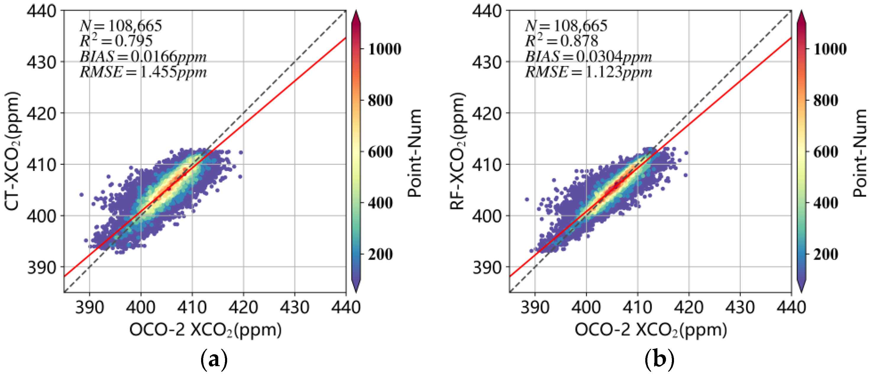
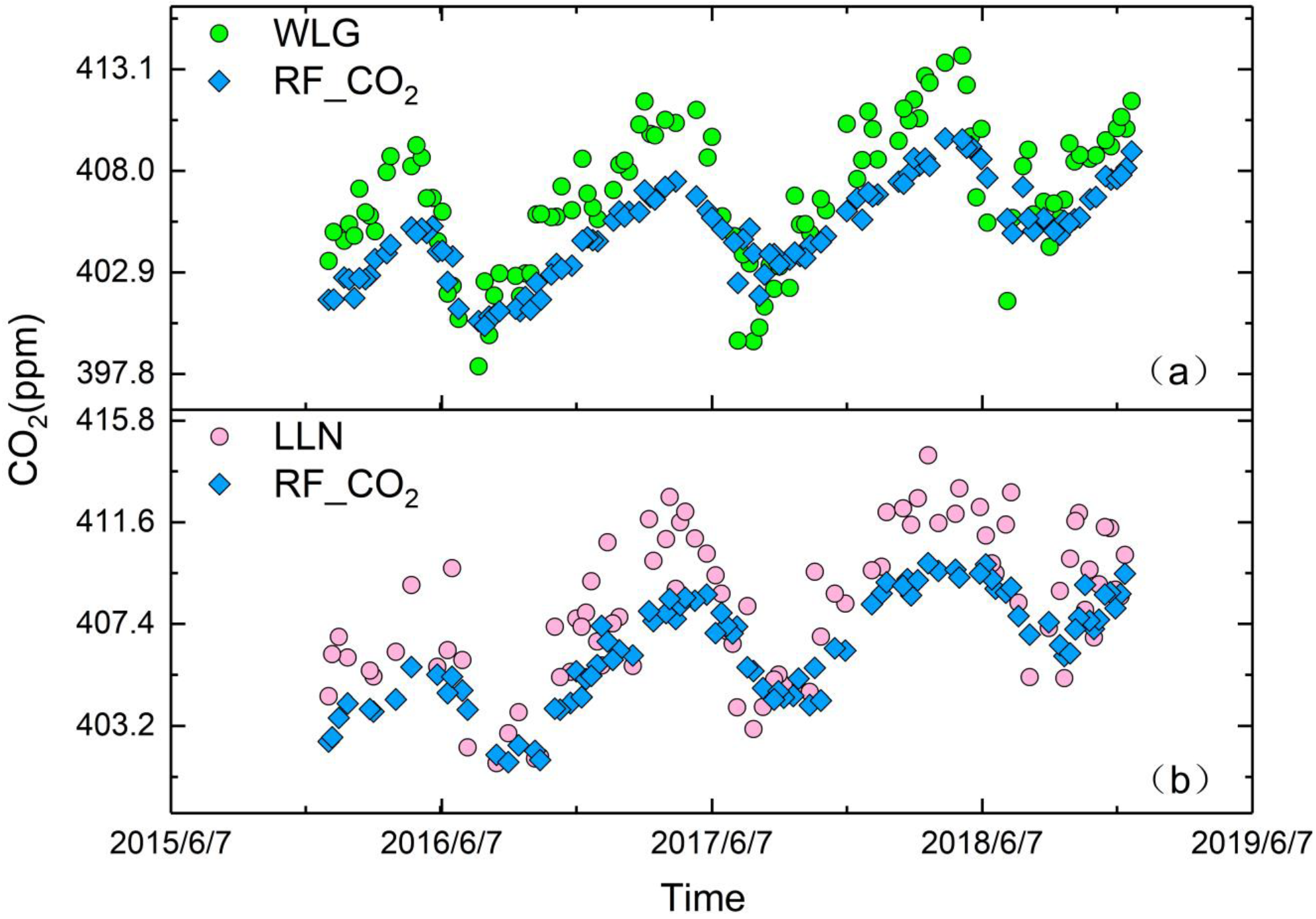
3.2. Comparison of RF XCO2 and CT XCO2

From 2016 to 2018, the national average of RF XCO2 was 0.237 ppm lower than CT XCO2 (Figure 3d), but the national annual mean difference showed an increasing trend, from −0.108 ppm in 2016 to 0.239 ppm in 2018 (Figure 3a–c). In terms of spatial distribution, ∆XCO2 (∆XCO2 = CT XCO2 − RF XCO2) was relatively high in East China, Central China, South China, and Northeast China. The CT XCO2 value was higher than the RF XCO2 value. ∆XCO2 was significantly lower in southern Xinjiang, indicating that CT XCO2 was significantly underestimated in this region. However, ∆XCO2 was relatively small in North China, Southwest China, and most parts of Northwest China, indicating that the CT XCO2 value was relatively accurate and presented little difference from the RF XCO2 value. The main reason for the above phenomenon is that CT XCO2 relies heavily on ground data; however, China currently has few ground monitoring stations with uneven distribution. China is preparing to install more ground monitoring stations, which will help to conduct better monitoring in the future, allowing for further Validation and improvement of Carbon Tracker models.
The RF XCO2 fit the OCO-2 XCO2 well, and thus the spatiotemporal distribution of ∆XCO2 may serve to represent the difference between OCO-2 XCO2 and CT XCO2 visually. In contrast, the differences between CT XCO2 and OCO-2 XCO2 n East China, Central China, South China, Northeast China, and southern Xinjiang were significantly larger, while those in North China, Southwest China, and Northwest China were relatively small. The comparison results indicated that there are still high uncertainties in CT XCO2, which may be mainly due to the errors in the emission inventory and the small number of ground observation stations. This result may also be due to the high uncertainty and coarse spatial resolution (3° × 2°) of CT XCO2, making it insufficient to display the detailed spatial distribution of XCO2, especially in small areas. Therefore, the XCO2 data set, with full coverage and high spatial resolution, is of great value for monitoring the distribution of carbon sources and sinks in China.

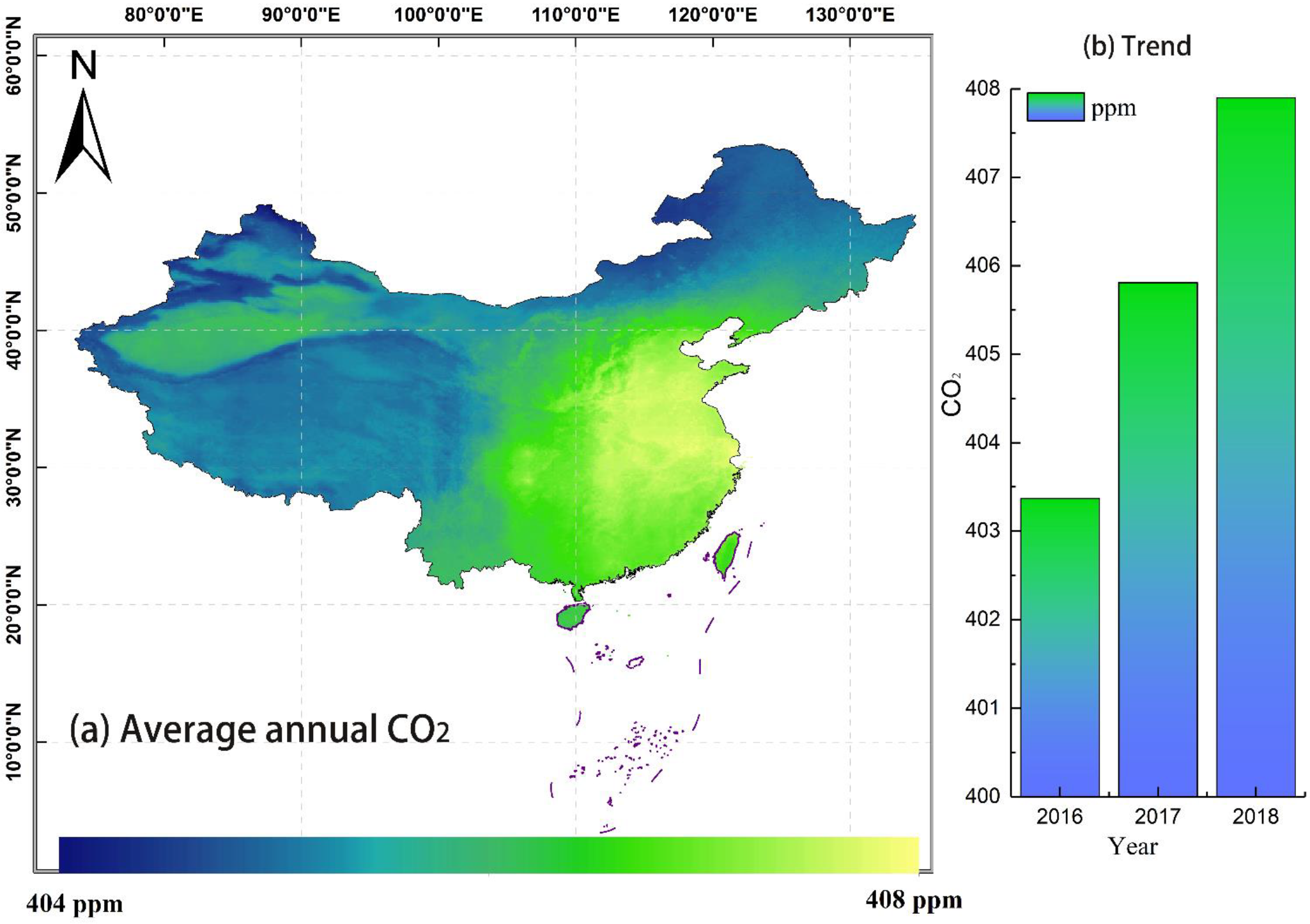
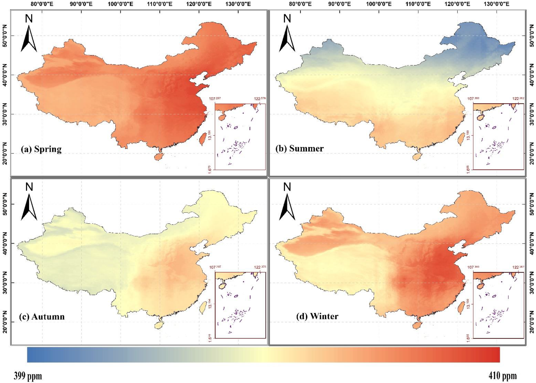
3.3. Spatial Distribution of RF XCO2

From 2016 to 2018, the multi-year average of RF XCO2 in China was 405.86 ± 1.73 ppm (Figure 4a), with the highest level in East China (406.94 ± 0.65 ppm) and the lowest level in Northwest China (405.56 ± 1.43 ppm). CO2 emissions are often related to intensive human activities. East China and Central China not only possess large populations but also have developed economies and intensive human activities. This is also the main reason for the high XCO2 observed in East and Central China. XCO2 was also relatively high in parts of North China, mainly due to the intensive human activities in the Beijing—Tianjin—Hebei region, the use of centralized heating for a long period of time in winter, high CO2 emissions, and cold and dry winters, resulting in the low photosynthetic efficiency of vegetation. Inner Mongolia has low population density and lush vegetation, so XCO2 is relatively low in this region [37]. In South China, the economy is relatively developed and there are many human activities; however, due to the warm and humid climate, the vegetation coverage rate is relatively high, and its photosynthetic carbon fixation rate is relatively high, causing the level of XCO2 to be moderate [35]. For Northeast and Northwest China, the population density is low, and carbon emissions from fossil fuel combustion and biomass combustion are relatively low, causing the XCO2 to be low. The southwest region has a moderate population, but the vegetation is lush, the climate is humid, and the photosynthetic efficiency of the vegetation is high, such that the XCO2 is low. Compared with CT XCO2, RF XCO2 presented a more detailed and accurate spatiotemporal distribution. Compared with OCO-2 satellite data, due to clouds or other reasons, there are a lot of missing data, making it difficult to directly apply to carbon source and carbon sink monitoring, while RF XCO2 can achieve full coverage of XCO2 data, allowing for more effective monitoring of carbon sources and sinks.
From 2016 to 2018, the national RF XCO2 increased from 403.37 to 407.90 ppm (see Figure 4b), with an average rate of 2.265 ppm/year. The XCO2 growth rates in North China, Southwest China, and East China were all higher than the national average rate (2.315 ppm/year, 2.303 ppm/year, and 2.267 ppm/year, respectively), while the XCO2 growth rates in Northwest, Northeast, Central, and South China were lower than the national average rate (2.263 ppm/year, 2.222 ppm/year, 2.195 ppm/year and 2.178 ppm/year, respectively). Although XCO2 was still increasing, its growth rate gradually slowed down, from 2.44 ppm/year in 2016–2017 to 2.09 ppm/year in 2017–2018, which may be due to the promotion of low-carbon life and the use of clean energy.
From 2016 to 2018, the national averages of RF XCO2 in spring (Figure 5a), summer (Figure 5b), autumn (Figure 5c), and winter (Figure 5d) were 407.76 ± 1.72, 403.15 ± 3.36, 404.86 ± 1.71 and 406.90 ± 2.50 ppm, respectively. From the perspective of seasonal distribution, in most regions of China, XCO2 in spring was higher than that in summer, consistent with the results of previous studies [35,38]. In spring, the average seasonal value of XCO2 in Northeast China, East China, North China, Central China, South China, and Northwest China was higher than 407 ppm; meanwhile, in summer, the average seasonal value of XCO2 in Northeast China, North China, Northwest China, and parts of Central China was lower than 405 ppm. The reason may be that the summer was warm and humid, vegetation photosynthesis was strong, and a large amount of CO2 was absorbed by plants, resulting in a decrease of 4.61 ppm in the national average in summer compared with spring. In winter, due to the cold and dry climate, plant respiration is stronger than photosynthesis, resulting in a large amount of CO2 being accumulated in the atmosphere, leading to generally higher XCO2 than that in autumn and summer. In addition, most areas in northern China use fossil fuels or biomass for heating in winter, producing a large amount of CO2. This is why the seasonal variations in North China, Northeast China, and Northwest China are greater than those in the South. In summary, the main reasons for the seasonal variation of XCO2 may be plant photosynthesis and human activities (mainly including fossil fuel consumption and agricultural production) [35,39].

4. Conclusions

Based on OCO2 XCO2, CT XCO2, and multivariate geographic data, the full-coverage spatiotemporal distribution of daytime XCO2 in China from 2016 to 2018 was obtained using a Random Forest machine learning model. Compared with CT XCO2, having a coarse spatial resolution (3° × 2°), RF XCO2 with a high spatial resolution (0.1° × 0.1°) showed more detailed spatial variation, indicating that it may be used to identify potentially important carbon sources and sinks in further research. The RF-XCO2 data set constructed in this study better revealed the distribution of XCO2 in China. In terms of spatial distribution, the highest multi-year average RF XCO2 value was in East China (406.94 ± 0.65 ppm), while the lowest was in Northwest China (405.56 ± 1.43 ppm). In view of the different levels of CO2 emissions in different geographical regions, it is necessary to reduce CO2 emissions in East China, Central China and parts of North China or to establish an effective carbon trading market to achieve a dynamic carbon emission balance in different regions. In terms of time, from 2016 to 2018, the annual XCO2 in China continued to increase, but the growth rate showed a downward trend. In terms of seasonal trends, the multi-year average XCO2 in spring was the highest (407.76 ± 1.72 ppm), while that in summer was the lowest (403.15 ± 3.36 ppm). In view of these inter-annual and seasonal changes, it is necessary to fully promote clean energy, replace fossil fuels and biomass fuels, and reduce seasonal changes within the year while maintaining a low growth rate. With the continuous launch of carbon monitoring satellites (e.g., GOSAT, OCO-2, and OCO-3), future multi-satellite combinations can better achieve data assimilation, which is expected to not only improve the quality of data but also extend the timeframe for XCO2 prediction.

Author Contributions

Conceptualization, S.H.; methodology, S.H., Y.Y. and Z.W.; investigation, Y.Y., Z.W., L.L. and Z.Z.; writing—original draft preparation, S.H., Z.W. and H.D.; writing—review and editing, S.H. and C.Z. All authors have read and agreed to the published version of the manuscript.

Funding

This research was funded by Open Funding of Zhejiang Key Laboratory of Ecological and Environmental Big Data (No.EED-2022-07), Fenghua Science and Technology Plan Project (202209204), and National Natural Science Foundation of China (52079101).

Institutional Review Board Statement

Not applicable.

Informed Consent Statement

Not applicable.

Data Availability Statement

All data used in this study, including satellite and ground data, are from sources providing the data freely available through the internet.

Conflicts of Interest

The authors declare no conflict of interest.

References

  1. IPCC. Climate Change 2021: The Physical Science Basis; Contribution of Working Group I to the Sixth Assessment Report of the Intergovernmental Panel on Climate Change; Cambridge Press: Cambridge, UK, 2021. [Google Scholar]
  2. Edenhofer, O.; Seyboth, K. Intergovernmental panel on climate change (IPCC). Encycl. Energy Nat. Resour. Environ. Econ. 2013, 26, 48–56. [Google Scholar]
  3. Hungershoefer, K.; Breon, F.M.; Peylin, P.; Chevallier, F.; Rayner, P.; Klonecki, A.; Houweling, A.; Marshall, J. Evaluation of various observing systems for the global monitoring of CO2 surface fluxes. Atmos. Chem. Phys. 2010, 10, 10503–10520. [Google Scholar] [CrossRef] [Green Version]
  4. Butz, A.; Hasekamp, O.P.; Frankenberg, C.; Aben, I. Retrievals of atmospheric CO2 from simulated space-borne measurements of backscattered near-infrared sunlight: Accounting for aerosol effects. Appl. Opt. 2009, 48, 3322–3336. [Google Scholar] [CrossRef] [Green Version]
  5. Bovensmann, H.; Burrows, J.P.; Buchwitz, M.; Frerick, J.; Noël, S.; Rozanov, V.V.; Chance, K.V.; Goede, A.P.H. SCIAMACHY—Mission objectives and measurement modes. J. Atmos. Sci. 1999, 56, 127–150. [Google Scholar] [CrossRef]
  6. Zhao, M.; Yue, T.; Zhang, X.; Sun, J.; Jiang, L.; Wang, C. Fusion of multi-source near-surface CO2 concentration data based on high accuracy surface modeling. Atmos. Pollut. Res. 2017, 8, 1170–1178. [Google Scholar]
  7. Ballav, S.; Naja, M.; Patra, P.K.; Machida, T.; Mukai, H. Assessment of spatio-temporal distribution of CO2 over greater Asia using the WRF–CO2 model. J. Earth Syst. Sci. 2020, 129, 80. [Google Scholar] [CrossRef]
  8. Andres, R.J.; Boden, T.A.; Bréon, F.M.; Ciais, P.; Davis, S.; Erickson, D.; Gregg, J.S.; Jacobson, A.; Marland, G.; Miller, J.; et al. A synthesis of carbon dioxide emissions from fossil-fuel combustion. Biogeosciences 2012, 9, 1845–1871. [Google Scholar] [CrossRef] [Green Version]
  9. Wunch, D.; Wennberg, P.O.; Osterman, G.; Fisher, B.; Naylor, B.; Roehl, C.M.; O’Dell, C.; Mandrake, L.; Viatte, C.; Griffith, D.W.; et al. Comparisons of the Orbiting Carbon Observatory-2 (OCO-2) XCO2measurements with TCCON. Atmos. Meas. Tech. Discuss. 2017, 10, 2209–2238. [Google Scholar] [CrossRef] [Green Version]
  10. Liang, A.; Gong, W.; Han, G.; Xiang, C. Comparison of Satellite-Observed XCO2 from GOSAT, OCO-2, and Ground-Based TCCON. Remote Sens. 2017, 9, 1033. [Google Scholar] [CrossRef] [Green Version]
  11. Wu, L.; Meijer, Y.; Sierk, B.; Hasekamp, O.; Butz, A.; Landgraf, J. XCO2 observations using satellite measurements with moderate spectral resolution: Investigation using GOSAT and OCO-2 measurements. Atmos. Meas. Tech. 2020, 13, 713–729. [Google Scholar] [CrossRef] [Green Version]
  12. Nguyen, H.; Katzfuss, M.; Cressie, N.; Braverman, A. Spatio-temporal data fusion for very large remote sensing datasets. Technometrics 2014, 56, 174–185. [Google Scholar] [CrossRef]
  13. Tomosada, M.; Kanefuji, K.; Matsumoto, Y.; Tsubaki, H. A Prediction Method of the Global Distribution Map of CO2 Column Abundance Retrieved from GOSAT Observation Derived from Ordinary Kriging. In Proceedings of the ICROS-SICE International Joint Conference 2009, Fukuoka International Congress Center, Fukuoka, Japan, 18–21 August 2009. [Google Scholar]
  14. Zeng, Z.; Lei, L.; Guo, L.; Zhang, L.; Zhang, B. Incorporating temporal variability to improve geostatistical analysis of satellite-observed CO2 in China. Chin. Sci. Bull. 2013, 58, 1948–1954. [Google Scholar] [CrossRef] [Green Version]
  15. Hammerling, D.M.; Michalak, A.M.; Kawa, S.R. Mapping of CO2 at high spatiotemporal resolution using satellite observations: Global distributions from OCO-2. J. Geophys. Res. Atmos. 2012, 117, D06306. [Google Scholar] [CrossRef]
  16. Guo, M.; Wang, X.; Li, J.; Yi, K.; Zhong, G.; Tani, H. Assessment of global carbon dioxide concentration using MODIS and GOSAT data. Sensors 2012, 12, 16368–16389. [Google Scholar] [CrossRef] [Green Version]
  17. Siabi, Z.; Falahatkar, S.; Alavi, S.J. Spatial distribution of XCO2 using OCO-2 data in growing seasons. J. Environ. Manag. 2019, 244, 110–118. [Google Scholar] [CrossRef]
  18. Girach, I.A.; Ponmalar, M.; Murugan, S.; Rahman, P.A.; Babu, S.S.; Ramachandran, R. Ramachandran. Applicability of Machine Learning Model to Simulate Atmospheric CO₂ Variability. IEEE Trans. Geosci. Remote Sens. 2022, 60, 4107306. [Google Scholar] [CrossRef]
  19. He, C.; Ji, M.; Li, T. Deriving Full-Coverage and Fine-Scale XCO2 Across China Based on OCO-2 Satellite Retrievals and CarbonTracker Output. Geophys. Res. Lett. 2022, 49, e2022GL098435. [Google Scholar] [CrossRef]
  20. Li, J.; Jia, K.; Wei, X.; Xia, M.; Chen, Z.; Yao, Y.; Zhang, X.; Jiang, H.; Yuan, B.; Tao, G.; et al. High-spatiotemporal resolution mapping of spatiotemporally continuous atmospheric CO2 concentrations over the global continent. Int. J. Appl. Earth Obs. Geoinf. 2022, 108, 102743. [Google Scholar] [CrossRef]
  21. Wang, W.; He, J.; Feng, H.; Jin, Z. High-Coverage Reconstruction of XCO2 Using Multisource Satellite Remote Sensing Data in Beijing–Tianjin–Hebei Region. Int. J. Environ. Res. Public Health 2022, 19, 10853. [Google Scholar] [CrossRef]
  22. Zhang, L.; Li, T.; Wu, J. Deriving gapless CO2 concentrations using a geographically weighted neural network: China, 2014–2020. Int. J. Appl. Earth Obs. Geoinf. 2022, 114, 103063. [Google Scholar] [CrossRef]
  23. Nassar, R.; Hill, T.G.; McLinden, C.A.; Wunch, D.; Jones, D.B.A.; Crisp, D. Quantifying CO2 emissions from individual power plants from space. Geophys. Res. Lett. 2017, 44, 10045–10053. [Google Scholar] [CrossRef] [Green Version]
  24. Jacobson, A.R.; Schuldt, K.N.; Miller, J.B.; Oda, T.; Tans, P.; Andrews, A.; Mund, J.; Ott, L.; Collatz, G.J.; Aalto, T.; et al. CarbonTracker CT2019B; NOAA Global Monitoring Laboratory: Boulder, CO, USA, 2020. [Google Scholar]
  25. Yang, L.; Meng, X.; Zhang, X. SRTM DEM and its application advances. Int. J. Remote Sens. 2011, 32, 3875–3896. [Google Scholar] [CrossRef]
  26. Tatem, A.J. WorldPop, open data for spatial demography. Sci. Data 2017, 4, 170004. [Google Scholar] [CrossRef]
  27. Friedl, M.A.; Sulla-Menashe, D. MODIS/Terra+Aqua Land Cover Type Yearly L3 Global 500m SIN Grid V006; NASA EOSDIS Land Processes DAAC: Sioux Falls, SD, USA, 2018. [Google Scholar]
  28. Didan, K. MOD13C1 MODIS/Terra Vegetation Indices 16-Day L3 Global 0.05Deg CMG V006; NASA EOSDIS Land Processes DAAC: Sioux Falls, SD, USA, 2015. [Google Scholar]
  29. Muñoz Sabater, J. ERA5-Land Hourly Data from 1981 to Present; Copernicus Climate Change Service (C3S) Climate Data Store (CDS): Brussels, Belgium, 2019. [Google Scholar]
  30. Breiman, L. Random forests. Mach. Learn. 2001, 45, 5–32. [Google Scholar] [CrossRef] [Green Version]
  31. Geurts, P.; Ernst, D.; Wehenkel, L. Extremely randomized trees. Mach. Learn. 2006, 63, 3–42. [Google Scholar] [CrossRef] [Green Version]
  32. Chen, T.; Guestrin, C. XGBoost: A scalable tree boosting system. In Proceedings of the ACM SIGKDD International Conference on Knowledge Discovery and Data Mining, Association for Computing Machinery, New York, NY, USA, 13–17 August 2016; pp. 785–794. [Google Scholar]
  33. Ke, G.; Meng, Q.; Finley, T.; Wang, T.; Chen, W.; Ma, W.; Ye, Q.; Liu, T.Y. Lightgbm: A highly efficient gradient boosting decision tree. Adv. Neural Inf. Process. Syst. 2017, 30, 569–577. [Google Scholar]
  34. Dorogush, A.V.; Ershov, V.; Gulin, A. CatBoost: Gradient boosting with categorical features support. arXiv 2018, arXiv:1810.11363. [Google Scholar]
  35. Lv, Z.; Shi, Y.; Zang, S.; Sun, L. Spatial and Temporal Variations of Atmospheric CO2 Concentration in China and Its Influencing Factors. Atmosphere 2020, 11, 231. [Google Scholar] [CrossRef] [Green Version]
  36. Falahatkar, S.; Mousavi, S.M.; Farajzadeh, M. Spatial and temporal distribution of carbon dioxide gas using GOSAT data over IRAN. Environ. Monit. Assess. 2017, 189, 627. [Google Scholar] [CrossRef]
  37. Britter, R.E. Atmospheric Dispersion of Dense Gases. Annu. Rev. Fluid Mech. 1989, 21, 317–344. [Google Scholar] [CrossRef]
  38. Bie, N.; Lei, L.; He, Z.; Zeng, Z.; Liu, L.; Zhang, B.; Cai, B. Specific patterns of XCO2 observed by GOSAT during 2009–2016 and assessed with model simulations over China. Sci. China Earth Sci. 2020, 63, 384–394. [Google Scholar] [CrossRef]
  39. Xu, Y.; Ke, C.; Zhan, W.; Li, H.; Yao, L. Variations in satellite-derived carbon dioxide over different regions of China from 2003 to 2011. Atmos. Environ. 2017, 150, 379–388. [Google Scholar] [CrossRef]
Figure 1. Relationship between OCO-2 XCO2 and CT XCO2 (a) resampled to 0.1° × 0.1° by inverse distance-weighted interpolation, and RF XCO2 (b) predicted by the Random Forest model in sample-based cross-validation. The red dotted line represents the fitted line, while the dashed black line indicates a 1:1 relationship.
Atmosphere 14 00436 g001
Figure 2. Comparison of RF-CO2 observation data with WLG (a) and LLN (b) station observations.
Atmosphere 14 00436 g002
Figure 3. Spatial distribution of the annual mean difference between CT XCO2 and RF XCO2 from 2016 to 2018 (ac) and the multi-year mean difference between CT XCO2 and RF XCO2 (d).
Atmosphere 14 00436 g003
Figure 4. Spatial distribution of multi-year averages RF XCO2 (a) and 2016—2018 annual averages RF XCO2 (b).
Atmosphere 14 00436 g004
Figure 5. Spatial distribution of multi-year Spring (a), Summer (b), Autumn (c), and Winter (d) averages of RF XCO2 from 2016 to 2018.
Atmosphere 14 00436 g005
Table 1. Auxiliary data and related information.
Data SourceTypeSpatial ResolutionTime Resolution
Carbon TrackerXCO23° × 2°3 h
MODISNDVI0.05° × 0.05°8 d
Land-Use (LU)500 m × 500 m1 y
ERA-52 m temperature (t2m)0.25° × 0.25°1 h
2 m dewpoint temperature (d2m)
Surface pressure (sp)
10 m v-component of wind (v10)
10 m u-component of wind (u10)
World PopPopulation density (pop)1 km × 1 km1 y
SRTMDEM90 m × 90 m-
Table 2. Comparison of prediction performance of different machine learning models.
ModelCross-Validation R2RMSE (ppm)MAE (ppm)
RF0.8781.1230.867
ERT0.8451.2610.931
XGB0.8411.2790.952
LGB0.8321.3120.981
CatBoost0.8451.2610.935
Table 3. XCO2 prediction model variable importance distribution.
VariableImportanceVariableImportance
Longitude2.03%u100.68%
Latitude2.23%v100.72%
CT XCO283.08%DEM1.51%
d2m2.72%pop0.81%
t2m3.12%LU0.2%
sp1.99%NDVI0.91%
Disclaimer/Publisher’s Note: The statements, opinions and data contained in all publications are solely those of the individual author(s) and contributor(s) and not of MDPI and/or the editor(s). MDPI and/or the editor(s) disclaim responsibility for any injury to people or property resulting from any ideas, methods, instructions or products referred to in the content.

