


Uncertainty Analysis of Remote Sensing Underlying Surface in Land–Atmosphere Interaction Simulated Using Land Surface Models


Abstract
1. Introduction
2. Data and Methods
2.1. Community Land Model (CLM4.5) and Its Underlying Surface Dataset
2.2. ESACCI Underlying Surface Dataset
2.3. Processing of ESACCI Underlying Dataset
2.4. Experimental Design
3. Results and Discussion
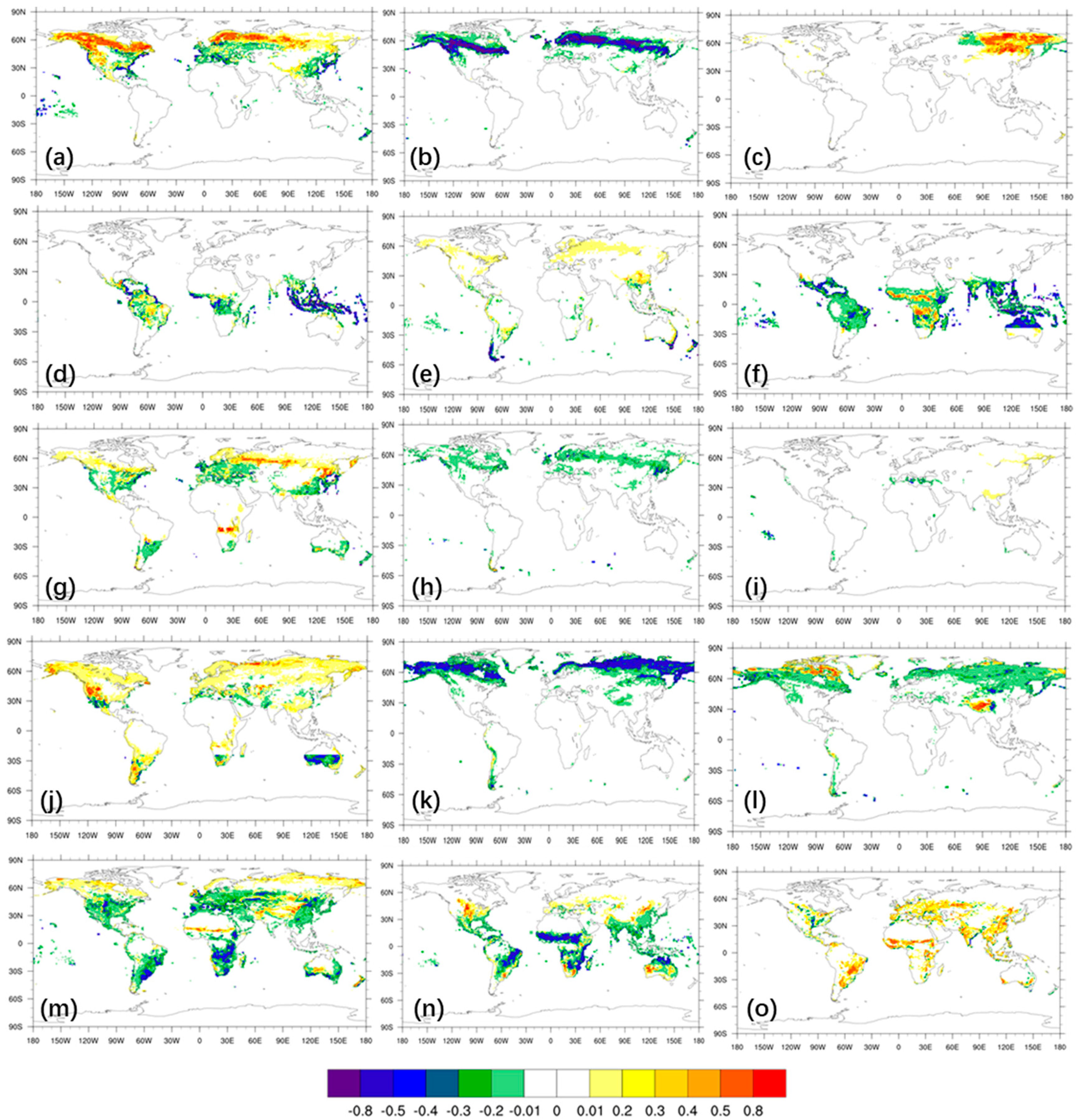
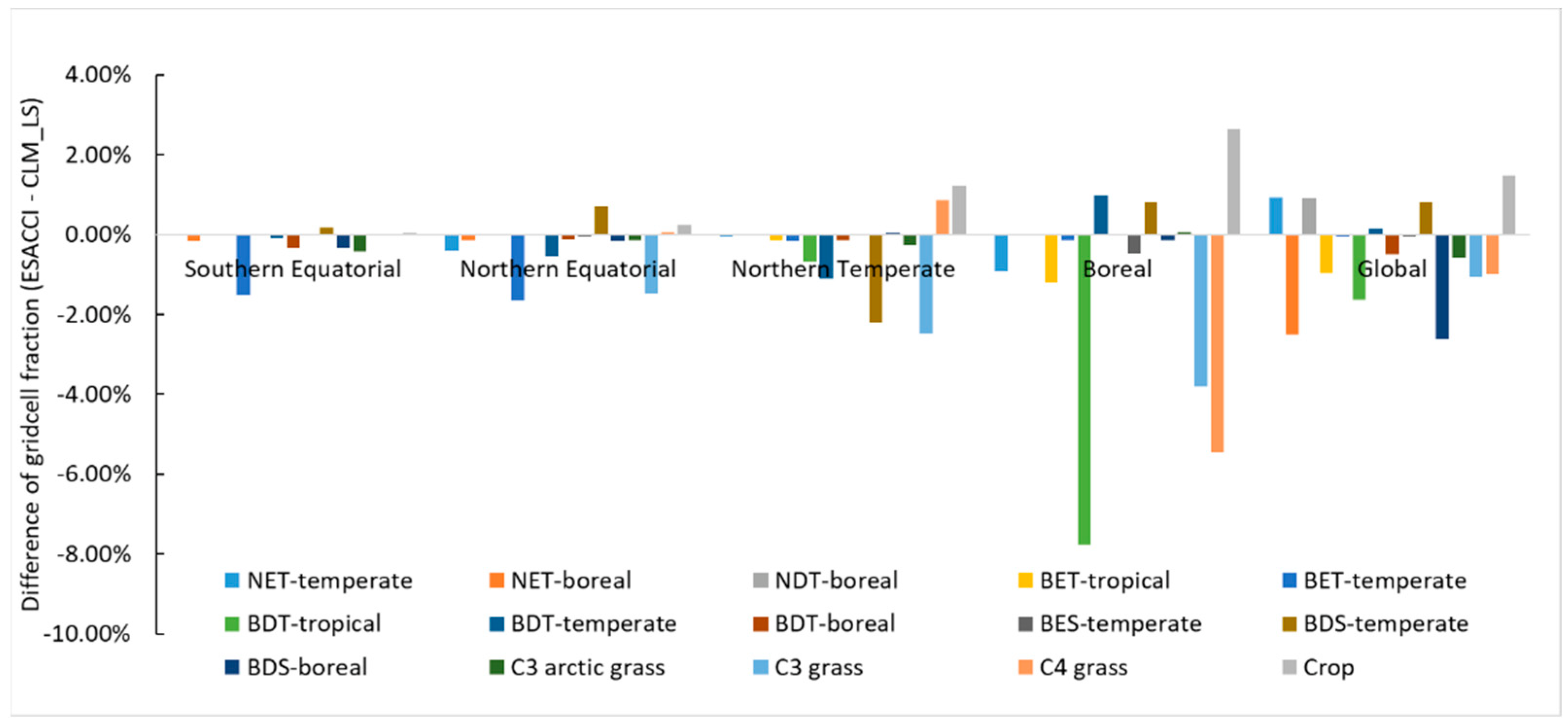
3.1. Differences in Underlying Surfaces
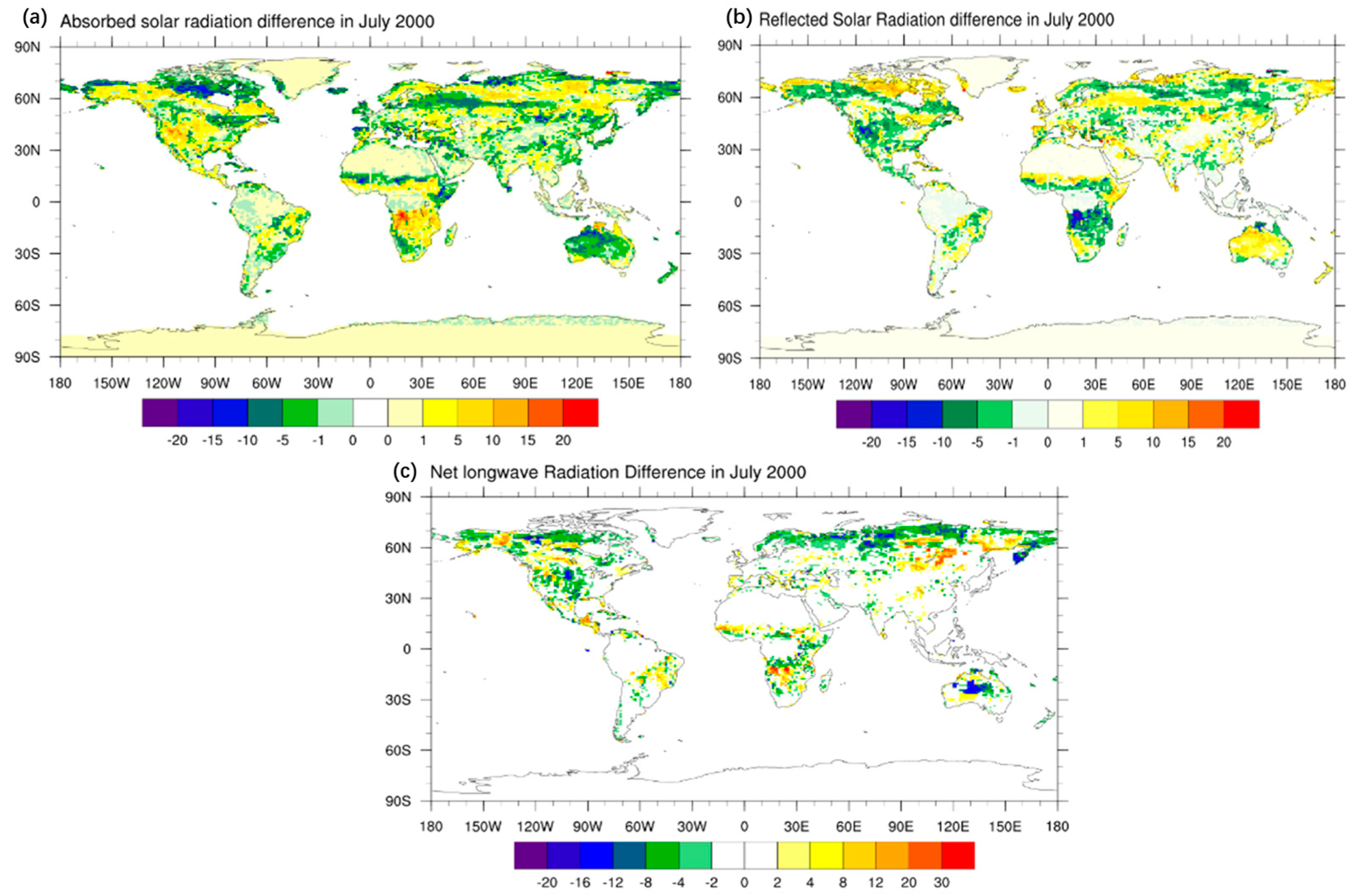
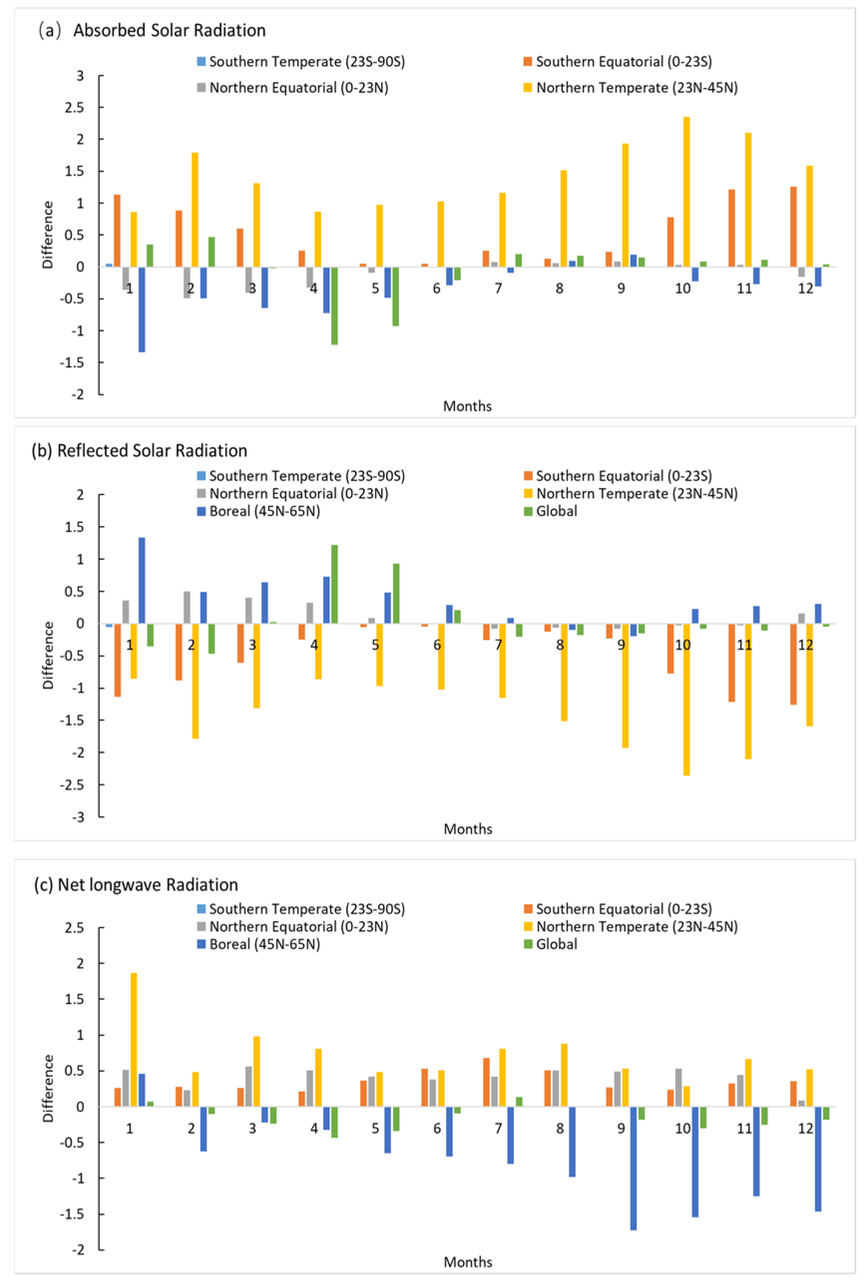
3.2. Radiation
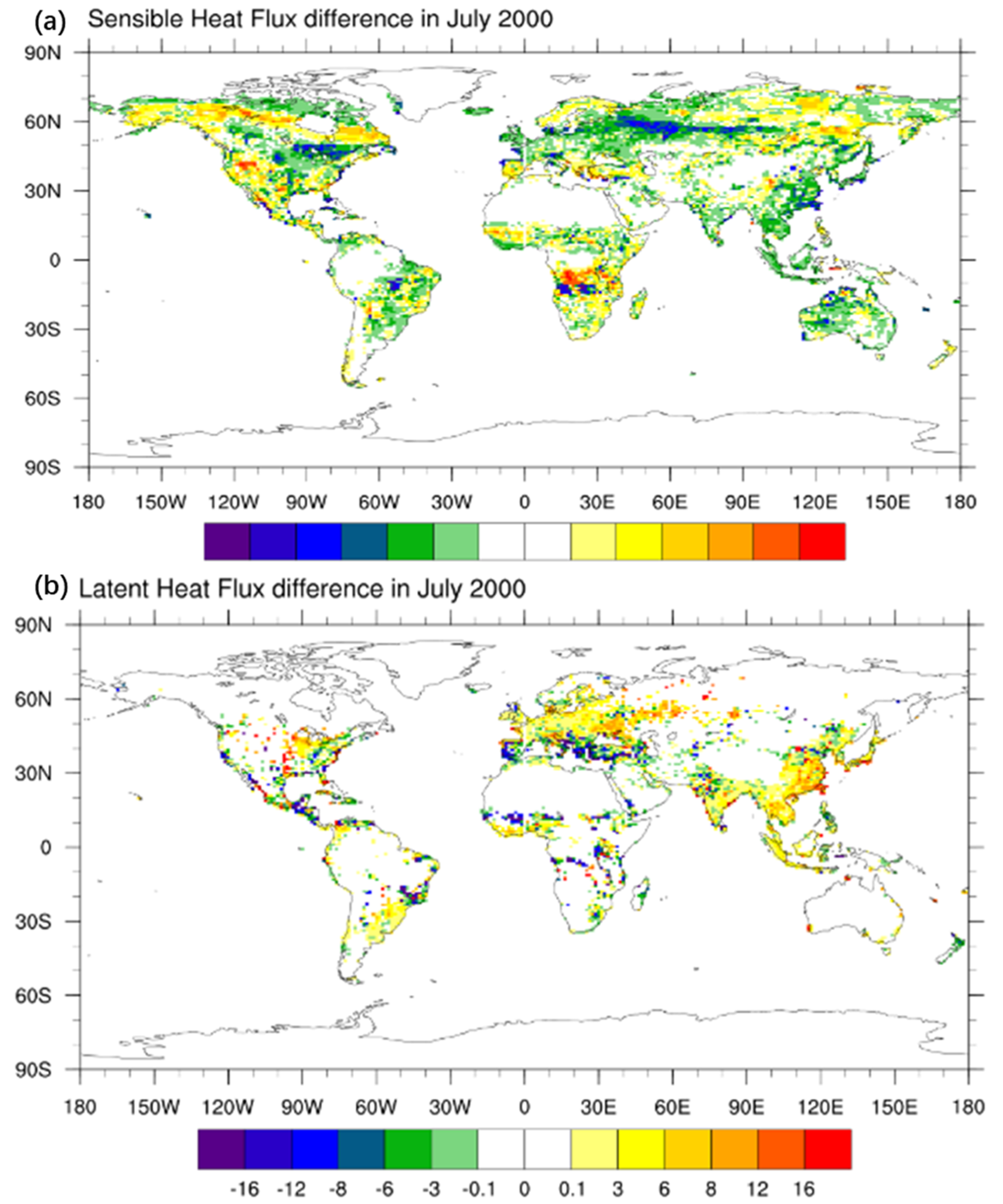
3.3. Heat Fluxes
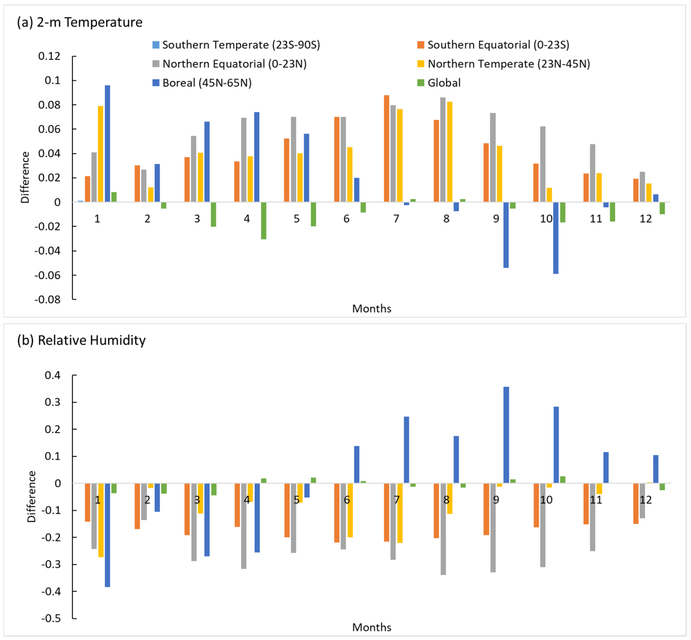
3.4. Response of Micro-Meteorological Elements
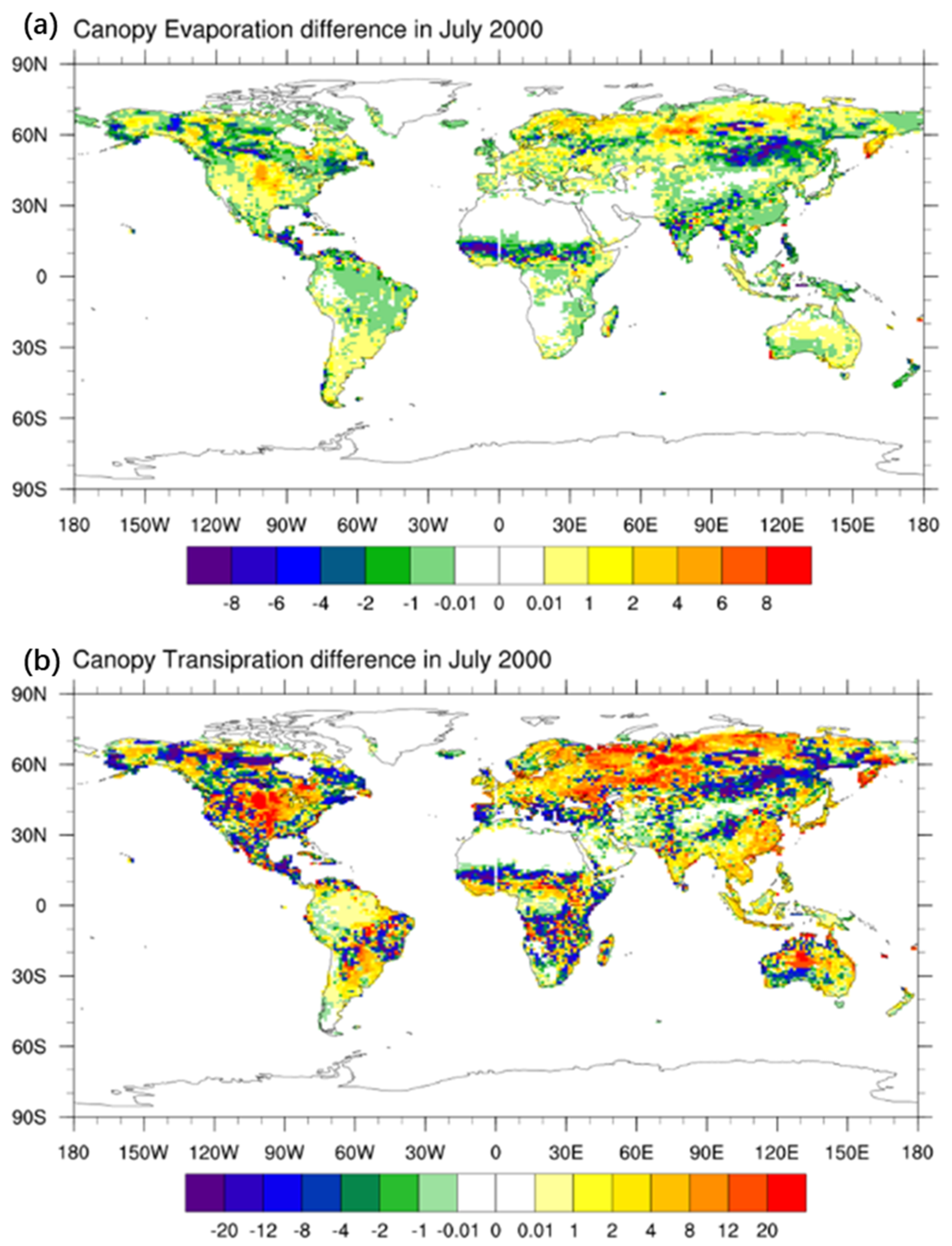
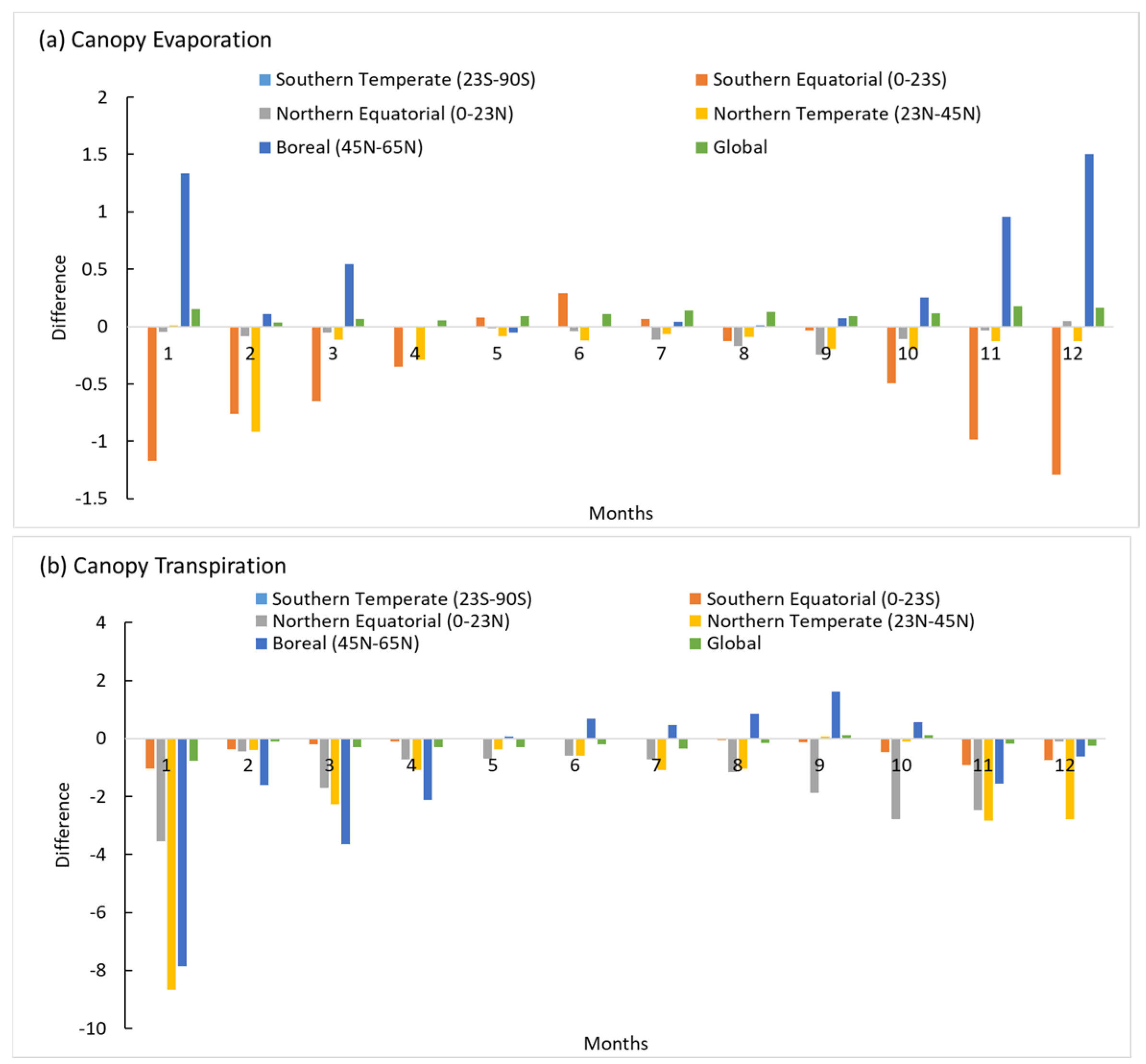
3.5. Response of Hydrological Variables
4. Discussion and Conclusions
- The proportion of cropland distribution in ESACCI data is essentially larger than that in CLM_LS data globally, and it can reach more than 50% locally.
- The model concluded that the difference in parameters is related to the difference in cropland distribution, and the difference in absorbed solar radiation and sensible heat flux has an obvious response to the difference in cropland distribution.
- Differences in the distribution of cropland bring about different degrees of changes in climate parameters. The uncertainty of the data can be transmitted to the model operation process through the data themselves, which brings uncertainty to the model results and affects the climate simulation.
Author Contributions
Funding
Institutional Review Board Statement
Informed Consent Statement
Data Availability Statement
Acknowledgments
Conflicts of Interest
References
- Desai, A.R.; Paleri, S.; Mineau, J.; Kadum, H.; Wanner, L.; Mauder, M.; Butterworth, B.J.; Durden, D.J.; Metzger, S. Scaling land-atmosphere interactions: Special or fundamental? J. Geophys. Res. Biogeosci. 2022, 127, e2022JG007097. [Google Scholar] [CrossRef]
- Bonan, G.B. Sensitivity of a GCM simulation to inclusion of inland water surfaces. J. Clim. 1995, 8, 14. [Google Scholar] [CrossRef]
- Berg, A.; Findell, K.; Lintner, B.; Giannini, A.; Seneviratne, S.I.; van den Hurk, B.; Lorenz, R.; Pitman, A.; Hagemann, S.; Meier, A.; et al. Land-atmosphere feedbacks amplify aridity increase over land under global warming. Nat. Clim. Change 2016, 6, 869–874. [Google Scholar] [CrossRef]
- Santanello, J.A., Jr.; Dirmeyer, P.A.; Ferguson, C.R.; Findell, K.L.; Tawfik, A.B.; Berg, A.; Ek, M.; Gentine, P.; Guillod, B.P.; van Heerwaarden, C.; et al. Land-atmosphere interactions: The LoCo perspective. Bull. Am. Meteorol. Soc. 2018, 99, 1253–1272. [Google Scholar] [CrossRef]
- Green, J.K.; Seneviratne, S.I.; Berg, A.M.; Findell, K.L.; Hagemann, S.; Lawrence, D.M.; Gentine, P. Large influence of soil moisture on long-term terrestrial carbon uptake. Nature 2019, 565, 476–479. [Google Scholar] [CrossRef] [PubMed]
- Warrach-Sagi, K.; Ilgwersen, J.; Schwitalla, T.; Troost, C.; Aurbacher, J.; Jach, L.; Berger, T.; Streck, T.; Wulfmeyerl, V. Noah-MP With the generic crop growth model gecros in the WRF model: Effects of dynamic crop growth on land-atmosphere interaction. J. Geophys. Res. Atmos. 2022, 127, e2022JD036518. [Google Scholar] [CrossRef]
- Maruyama, A.; Kuwagata, T. Coupling land surface and crop growth models to estimate the effects of changes in the growing season on energy balance and water use of rice paddies. Agric. For. Meteorol. 2010, 150, 919–930, Erratum in Agric. For. Meteorol. 2021, 308–309, 108585. [Google Scholar] [CrossRef]
- Majumder, A.; Kingra, P.K.; Setia, R.; Singh, S.P.; Pateriya, B. Influence of land use/land cover changes on surface temperature and its effect on crop yield in different agro-climatic regions of Indian Punjab. Geocarto Int. 2020, 35, 663–686. [Google Scholar] [CrossRef]
- Liu, F.S.; Chen, Y.; Xiao, D.P.; Bai, H.Z.; Tao, F.L.; Ge, Q.S. Modeling crop growth and land surface energy fluxes in wheat-maize double cropping system in the North China Plain. Theor. Appl. Climatol. 2020, 142, 959–970. [Google Scholar] [CrossRef]
- Baker, J.C.A.; de Souza, D.C.; Kubota, P.Y.; Buermann, W.; Coelho, C.A.S.; Andrews, M.B.; Gloor, M.; Garcia-Carreras, L.; Figueroa, S.N.; Spracklen, D.V. An assessment of land-atmosphere interactions over South America using satellites, reanalysis, and two global climate models. J. Hydrometeorol. 2021, 22, 905–922. [Google Scholar] [CrossRef]
- Song, Y.Y.; Wei, J.F. Diurnal cycle of summer precipitation over the North China Plain and associated land-atmosphere interactions: Evaluation of ERA5 and MERRA-2. Int. J. Climatol. 2021, 41, 6031–6046. [Google Scholar] [CrossRef]
- Ma, Y.M.; Hu, Z.Y.; Xie, Z.P.; Ma, W.Q.; Wang, B.B.; Chen, X.L.; Li, M.S.; Zhong, L.; Sun, F.L.; Gu, L.L.; et al. A long-term (2005–2016) dataset of hourly integrated land-atmosphere interaction observations on the Tibetan Plateau. Earth Syst. Sci. Data 2020, 12, 2937–2957. [Google Scholar] [CrossRef]
- Dare-Idowu, O.; Jarlan, L.; Le-Dantec, V.; Rivalland, V.; Ceschia, E.; Boone, A.; Brut, A. Hydrological Functioning of maize crops in Southwest France using eddy covariance measurements and a land surface model. Water 2021, 13, 1481. [Google Scholar] [CrossRef]
- Zhang, Z.; Chen, F.; Barlage, M.; Bortolotti, L.E.; Famiglietti, J.; Li, Z.; Ma, X.; Li, Y. Cooling effects revealed by modeling of wetlands and land-atmosphere interactions. Water Resour. Res. 2022, 58, e2021WR030573. [Google Scholar] [CrossRef]
- Imran, H.M.; Hossain, A.; Shammas, M.I.; Das, M.K.; Islam, M.R.; Rahman, K.; Almazroui, M. Land surface temperature and human thermal comfort responses to land use dynamics in Chittagong city of Bangladesh. Geomat. Nat. Haz. Risk 2022, 13, 2283–2312. [Google Scholar] [CrossRef]
- Mahmood, R.; Pielke, R.A.; Hubbard, K.G.; Niyogi, D.; Bonan, G.; Lawrence, P.; McNider, R.; McAlpine, C.; Etter, A.; Gameda, S.; et al. Impacts of land use/land cover change on climate and future research priorities. Bull. Am. Meteorol. Soc. 2010, 91, 37–46. [Google Scholar] [CrossRef]
- Zhai, J.; Liu, R.G.; Liu, J.Y.; Huang, L.; Qin, Y.W. Human-induced landcover changes drive a diminution of land surface albedo in the Loess Plateau (China). Remote Sens. 2015, 7, 2926–2941. [Google Scholar] [CrossRef]
- Fu, T.M.; Zhang, L.; Chen, B.W.; Yan, M. Human disturbance on the land surface environment in tropical islands: A remote sensing perspective. Remote Sens. 2022, 14, 2100. [Google Scholar] [CrossRef]
- Hu, S.L.; Yu, B.; Luo, S.; Zhuo, R.R. Spatial pattern of the effects of human activities on the land surface of China and their spatial relationship with the natural environment (s10668-021-01871-6, 2021). Environ. Dev. Sustain. 2022, 24, 14421. [Google Scholar] [CrossRef]
- Yamada, T.J.; Pokhrel, Y. Effect of Human-induced land disturbance on subseasonal predictability of near-surface variables using an atmospheric general circulation model. Atmosphere 2019, 10, 725. [Google Scholar] [CrossRef]
- Xu, Z.; Mahmood, R.; Yang, Z.-L.; Fu, C.; Su, H. Investigating diurnal and seasonal climatic response to land use and land cover change over monsoon Asia with the Community Earth System Model. J. Geophys. Res. Atmos. 2015, 120, 1137–1152. [Google Scholar] [CrossRef]
- Okkan, U.; Kirdemir, U. Investigation of the behavior of an agricultural-operated dam reservoir under RCP scenarios of AR5-IPCC. Water Resour. Manag. 2018, 32, 2847–2866. [Google Scholar] [CrossRef]
- Pachauri, R.K.; Allen, M.R.; Barros, V.R.; Broome, J.; Cramer, W.; Christ, R.; Church, J.A.; Clarke, L.; Dahe, Q.; Dasgupta, P.; et al. Climate Change 2014: Synthesis Report. Contribution of Working Groups I, II and III to the Fifth Assessment Report of the Intergovernmental Panel on Climate Change; IPCC: Geneva, Switzerland, 2014; p. 151. [Google Scholar]
- Birch, E.L. Climate change 2014: Impacts, adaptation, and vulnerability. J. Am. Plann. Assoc. 2014, 80, 184–185. [Google Scholar] [CrossRef]
- Foley, J.A.; DeFries, R.; Asner, G.P.; Barford, C.; Bonan, G.; Carpenter, S.R.; Chapin, F.S.; Coe, M.T.; Daily, G.C.; Gibbs, H.K.; et al. Global consequences of land use. Science 2005, 309, 570–574. [Google Scholar] [CrossRef] [PubMed]
- Zhang, X.Z.; Wang, W.C.; Fang, X.Q.; Ye, Y.; Zheng, J.Y. Agriculture development-induced surface albedo changes and climatic implications across Northeastern China. Chin. Geogr. Sci. 2012, 22, 264–277. [Google Scholar] [CrossRef]
- Goldewijk, K.K. Estimating global land use change over the past 300 years: The HYDE database. Glob. Biogeochem. Cycles 2001, 15, 417–433. [Google Scholar] [CrossRef]
- Cao, F.Q.; Dan, L.; Ma, Z.G. Simulative study of the impact of the cropland change on the regional climate over China. Acta Meteorol. Sin. 2015, 73, 14. [Google Scholar]
- Ahmad, M.J.; Cho, G.H.; Kim, S.H.; Lee, S.; Adelodun, B.; Choi, K.S. Influence mechanism of climate change over crop growth and water demands for wheat-rice system of Punjab, Pakistan. J. Water Clim. Change 2021, 12, 1184–1202. [Google Scholar] [CrossRef]
- Aurbacher, J.; Parker, P.S.; Sanchez, G.A.C.; Steinbach, J.; Reinmuth, E.; Ingwersen, J.; Dabbert, S. Influence of climate change on short term management of field crops—A modelling approach. Agric. Syst. 2013, 119, 44–57. [Google Scholar] [CrossRef]
- Cheng, J.Q.; Yin, S.Y. Quantitative assessment of climate change impact and anthropogenic influence on crop production and food security in Shandong, Eastern China. Atmosphere 2022, 13, 1160. [Google Scholar] [CrossRef]
- Wu, G.X.; Lin, H.; Zou, X.L.; Liu, B.Q.; He, B. Research on global climate change and scientific data. Adv. Earth Sci. 2014, 29, 8. [Google Scholar]
- Fathololoumi, S.; Firozjaei, M.K.; Li, H.J.; Biswas, A. Surface biophysical features fusion in remote sensing for improving land crop/cover classification accuracy. Sci. Total Environ. 2022, 838, 156520. [Google Scholar] [CrossRef]
- Quaife, T.; Cripps, E. Bayesian analysis of uncertainty in the GlobCover 2009 land cover product at climate model grid scale. Remote Sens. 2016, 8, 314. [Google Scholar] [CrossRef]
- Meiyappan, P.; Jain, A.K. Three distinct global estimates of historical land-cover change and land-use conversions for over 200 years. Front. Earth Sci. 2012, 6, 122–139. [Google Scholar] [CrossRef]
- Lawrence, P.J.; Chase, T.N. Investigating the climate impacts of global land cover change in the community climate system model. Int. J. Climatol. 2010, 30, 2066–2087. [Google Scholar] [CrossRef]
- Madhusoodhanan, C.G.; Sreeja, K.G.; Eldho, T.I. Assessment of uncertainties in global land cover products for hydro-climate modeling in India. Water Resour. Res. 2017, 53, 1713–1734. [Google Scholar] [CrossRef]
- Lawrence, P.J.; Chase, T.N. Representing a new MODIS consistent land surface in the Community Land Model (CLM 3.0). J. Geophys. Res. Biogeosci. 2007, 112. [Google Scholar] [CrossRef]
- Ramankutty, N.; Foley, J.A. Estimating historical changes in land cover: North American croplands from 1850 to 1992. Glob. Ecol. Biogeogr. 1999, 8, 381–396. [Google Scholar] [CrossRef]
- Li, H.; Zhang, H.; Mamtimin, A.; Fan, S.; Ju, C. A new land-use dataset for the weather research and forecasting (WRF) model. Atmosphere 2020, 11, 350. [Google Scholar] [CrossRef]


| CLM_LS | ESACCI | ||
|---|---|---|---|
| 1 | Needleleaf evergreen tree–temperate (NET–temperate) | 10 | Cropland, rainfed |
| 2 | Needleleaf evergreen tree–boreal (NET–boreal) | 20 | Cropland, irrigated or post-flooding |
| 3 | Needleleaf deciduous tree–boreal (NDT–boreal) | 30 | Mosaic cropland/natural vegetation |
| 4 | Broadleaf evergreen tree–tropical (BET–tropical) | 40 | Mosaic natural vegetation/cropland |
| 5 | Broadleaf evergreen tree–temperate (BET–temperate) | 50 | Tree cover, broadleaved, evergreen, closed to open |
| 6 | Broadleaf deciduous tree–tropical (BDT–tropical) | 60 | Tree cover, broadleaved, deciduous, closed to open |
| 7 | Broadleaf deciduous tree–temperate (BDT–temperate) | 70 | Tree cover, Needleleaved, evergreen, closed to open |
| 8 | Broadleaf deciduous tree–boreal (BDT–boreal) | 80 | Tree cover, needleleaved, deciduous, closed to open |
| 9 | Broadleaf evergreen shrub–temperate (BES–temperate) | 90 | Tree cover, mixed leaf type |
| 10 | Broadleaf deciduous shrub–temperate (BDS–temperate) | 100 | Mosaic tree and shrub/herbaceous cover |
| 11 | Broadleaf deciduous shrub–boreal (BDS–boreal) | 110 | Mosaic herbaceous cover/tree and shrub |
| 12 | C3 arctic grass | 120 | Shrubland |
| 13 | C3 grass | 130 | Grassland |
| 14 | C4 grass | 140 | Lichens and mosses |
| 15 | Crop | 150 | Sparse vegetation |
| 0 | Bare soil | 160 | Tree cover, flooded, fresh or brackish water |
| 170 | Tree cover, flooded, Saline water | ||
| 180 | Shrub or herbaceous cover, flooded, fresh/saline/brackish water | ||
| 190 | Urban areas | ||
| 200 | Bare areas | ||
| 210 | Water bodies | ||
| 220 | Permanent snow and ice | ||
| 0 | No Data | ||
| No. | PFTs | ESACCI | Climate Rules |
|---|---|---|---|
| 1 | NET–temperate | 70 | Tc1 > −19 °C, and GDD2 > 1200 |
| 2 | NET–boreal | 70 | Tc ≤ −19 °C, or GDD ≤ 1200 |
| 3 | NDT–boreal | 80, 81, 82 | none |
| 4 | BET–tropical | 50 | Tc > 15.5 °C |
| 5 | BET–temperate | 50 | Tc ≤ 15.5 °C |
| 6 | BDT–tropical | 60, 61 | Tc > 15.5 °C |
| 7 | BDT–temperate | 60, 61 | −15 °C < Tc ≤ 15.5 °C, and GDD > 1200 |
| 8 | BDT–boreal | 60, 61 | Tc ≤ −15 °C, or GDD ≤ 1200 |
| 9 | BES–temperate | 11, 120, 121, 122 | Tc > −19 °C and GDD > 1200 and Pann3 > 520 nm and Pwin4 > 2/3 Pann |
| 10 | BDS–temperate | 11, 120, 121,122 | Tc > −19 °C and GDD > 1200 and (Pann ≤ 520 nm or Pwin ≤ 2/3 Pann) |
| 11 | BDS–boreal | 11, 120, 121, 122 | Tc ≤ −19 °C, or GDD ≤ 1200 |
| 12 | C3 arctic grass | 110, 130 | GDD < 1000 |
| 13 | C3 grass | 110, 130 | GDD > 1000 and (Tw5 ≤ 22 °C or Pmon6 ≤ 25 mm and for months with T > 22 °C) |
| 14 | C4 grass | 110, 130 | GDD > 1000 and (Tw > 22 °C and driest month Pmon > 25 mm) |
| 15 | Crop | 10, 20, 30 | None |
| Name | Model | Land Surface Types | Initial Condition | Spatial Resolution | Simulation PERIODS |
|---|---|---|---|---|---|
| CTL | CLM4.5CN | CLM_LS | CLM | 0.9 × 1.25 | 2000 |
| ESACCI | CLM4.5CN | ESACCI | CLM | 0.9 × 1.25 | 2000 |
Disclaimer/Publisher’s Note: The statements, opinions and data contained in all publications are solely those of the individual author(s) and contributor(s) and not of MDPI and/or the editor(s). MDPI and/or the editor(s) disclaim responsibility for any injury to people or property resulting from any ideas, methods, instructions or products referred to in the content. |
© 2023 by the authors. Licensee MDPI, Basel, Switzerland. This article is an open access article distributed under the terms and conditions of the Creative Commons Attribution (CC BY) license (https://creativecommons.org/licenses/by/4.0/).
Share and Cite
Ling, X.; Gao, H.; Gao, J.; Liu, W.; Tang, Z. Uncertainty Analysis of Remote Sensing Underlying Surface in Land–Atmosphere Interaction Simulated Using Land Surface Models. Atmosphere 2023, 14, 370. https://doi.org/10.3390/atmos14020370
Ling X, Gao H, Gao J, Liu W, Tang Z. Uncertainty Analysis of Remote Sensing Underlying Surface in Land–Atmosphere Interaction Simulated Using Land Surface Models. Atmosphere. 2023; 14(2):370. https://doi.org/10.3390/atmos14020370
Chicago/Turabian StyleLing, Xiaolu, Hao Gao, Jian Gao, Wenhao Liu, and Zeyu Tang. 2023. "Uncertainty Analysis of Remote Sensing Underlying Surface in Land–Atmosphere Interaction Simulated Using Land Surface Models" Atmosphere 14, no. 2: 370. https://doi.org/10.3390/atmos14020370
APA StyleLing, X., Gao, H., Gao, J., Liu, W., & Tang, Z. (2023). Uncertainty Analysis of Remote Sensing Underlying Surface in Land–Atmosphere Interaction Simulated Using Land Surface Models. Atmosphere, 14(2), 370. https://doi.org/10.3390/atmos14020370