Article

Bivariate Hazard Assessment of Combinations of Dry and Wet Conditions between Adjacent Seasons in a Climatic Transition Zone

1
College of Desert Control Science and Engineering, Inner Mongolia Agricultural University, Hohhot 010018, China
2
Institute of Water Resources for Pastoral Areas, Ministry of Water Resources, Hohhot 010020, China
3
Inner Mongolia Agricultural and Animal Husbandry Technology Extension Center, Hohhot 010018, China
4
State Key Laboratory of Eco-Hydraulics in Northwest Arid Region of China, Xi’an University of Technology, Xi’an 710048, China
*
Author to whom correspondence should be addressed.
Atmosphere 2023, 14(3), 437; https://doi.org/10.3390/atmos14030437
Submission received: 15 January 2023 / Revised: 8 February 2023 / Accepted: 20 February 2023 / Published: 22 February 2023
(This article belongs to the Topic Hydrology and Water Resources Management)

Abstract

:

Highlights

What are the main findings?
  • The HRB most frequently suffers from continued dryness followed by transition from dry-ness to wetness.
  • Dryness–wetness combinations generally occur more frequent under climate change.
  • Frequency of prolonged dryness/wetness escalates more rapidly than abrupt transition events.
What is the implication of the main finding?
  • The spatial and temporal preference of inter-seasonal dryness–wetness combinations are elucidated.
  • Bivariate hazard assessment of dryness–wetness combinations enriches water-related hazard atlas and facilitates more integrated mitigation planning.

Abstract

Accumulated evidence reminds one that abrupt transitions between dry and wet spells, though attracting less attention, have harmful influences upon global continents as extensively investigated droughts and floods. This study attempts to incorporate dryness–wetness transitions into the current hazard assessment framework through bivariate frequency analysis and causal attribution from a teleconnection perspective. In the study, regional dry and wet conditions are monitored using the multivariate standardized drought index (MSDI) which facilitates the integrated evaluation of water deficits/surplus from a combined viewpoint of precipitation (largely denoting the received atmospheric water) and runoff (representing an important source of surface water). On such a basis, a copula-based method is subsequently utilized to calculate joint return periods of dryness–wetness combinations in three (i.e., moderate, severe and extreme) severity scenarios. The changing frequency of diverse dryness–wetness combinations is also estimated under a changing climate using a 25-year time window. Furthermore, the cross-wavelet transform is applied to attribute variations in dry and wet conditions to large-scale climate indices, which benefits the early warning of dryness–wetness combinations by providing predictive information. A case study conducted during 1952–2010 in the Huai River basin (HRB)—a typical climatic transition zone in China—shows that the HRB is subject to prolonged dryness with the highest frequency, followed by the abrupt transition from dryness to wetness. Spatially, abrupt dryness–wetness transitions are more likely to occur in the southern and central parts of the HRB than in the rest of the proportion. The past half-century has witnessed the dominantly higher frequency of occurrence of dryness–wetness combinations under three severity scenarios. In particular, the occurrence of the continued dry/wetness escalates more rapidly than transition events under climate change. Moreover, a preliminary attribution analysis discloses the link of the dry and wet conditions in the HRB with climate indices, such as the El Niño southern oscillation, the Pacific decadal oscillation and the Arctic oscillation, as well as sunspot activities. The results of the study enrich the current atlas of water-related hazards, which may benefit more effective hazard mitigation and adaptation.

1. Introduction

Droughts and floods are the most common types of natural hazards, which result in disastrous consequences in many parts of the world. Statistics from the World Meteorological Organization indicate that over the period 2000–2019, droughts and floods, jointly accounting for 49% of the total number of disasters worldwide, triggered over 721,000 deaths and economic losses as high as USD 779 billion. Extensive studies on water-related hazard assessment, thereby, mainly focus on the monitoring of regional dry and wet spells, the risk assessment of droughts and floods and the quantification of their adverse influence upon human communities [1,2,3,4]. However, less attention has been paid to abrupt transitions between dry and wet spells. The occurrence of abrupt dryness–wetness transitions with high severity tends to cost more relief efforts than either individual drought or flood. The influential dryness–wetness transition events are noted to prevail in climatic transition zones, such as the middle-lower reach of the Yangtze River basin and the Huai River basin in China [5,6,7], as well as Texas transitioning from the arid southwest United States to the humid southeast United States [8,9]. Additionally, increasing evidence provides a reminder that the accelerated water cycle largely due to climate warming has resulted in a more frequent emergence of precipitation and streamflow extremes in many parts of the globe [10,11,12,13]. It is still unclear whether the increasing number of hydro-meteorological extremes has intensified risks of abrupt transitions between dryness and wetness in regions of concern. Therefore, there exists the growing need for the hazard assessment of abrupt dryness–wetness transitions, with the purpose of enriching the current water-related hazard atlas and facilitating the development of more integrated mitigation planning.
This study more generally takes into account combinations of dryness and wetness between adjacent seasons, which encompass four elements, namely mutual transitions between dryness and wetness, the prolonged dryness and the prolonged wetness. Diverse dryness–wetness combinations have been recently reported to happen with an ascending frequency over the Asian and American continents. In 2011, the middle-lower reach of the Yangtze River basin suffered from an abrupt transition from spring dryness to early summer wetness [14]. The precipitation anomalies were observed to vary from 60% below the long-term mean in May to 100% above the long-term mean in June. When the focus shifts to Texas of the U.S., a historic four-year dry spell ended up with a flood persisting for several weeks in May 2015. A more recent transition event was present in 2017 when one of the top ten driest autumns emerged in the wake of the Hurricane Harvey flood inundating Texas in August, which resulted in at least USD 125 billion in damage. The year 2017—following 1919, 1957 and 2015—subsequently became the fourth time when Texas was subject to the sudden shifting between dry and wet spells in the latest century. Cases of the continued dryness and wetness are reported as well. An inter-seasonal dry spell persisted from spring to autumn over the Huai River basin (HRB) in 1994, ultimately triggering economic losses up to RMB 16 billion, crop failure estimated to be 5.6 million metric tons and the drinking water shortage affecting 9 million people and 1.5 million livestock. In contrast, the Meiyu front together with the typhoon influence often brings intense rainfall to the HRB, which makes it historically vulnerable to prolonged wetness in summer and early autumn [15]. Therefore, listed cases with severe socio-economic influence remind one that diverse combinations of dryness and wetness between adjacent seasons ought to catch our sufficient attention.
Hazard assessment of dryness–wetness combinations primarily benefits from the accurate characterization of water anomalies. Univariate indices are widely used by existing studies to monitor water deficits and surplus, which include the standardized precipitation index (SPI), the standardized runoff index (SRI) and the standardized groundwater index [16]. Dry and wet spells identified by different types of univariate indices, however, often differ in their timing of onset, persistence and termination [17]. Water anomalies, in fact, represent the abnormal status of usable water resources from multiple sources, such as precipitation, runoff and groundwater [18]. A current consensus subsequently reached among researchers [18,19,20,21,22] highlights that dryness/wetness characterization exclusively based on a single hydro-meteorological variable is likely insufficient to support reliable hazard assessment and rational decision making. Nowadays, the monitoring of water anomalies is increasingly believed to be more appropriately conducted with consideration for changes in multiple water sources. Following the prevailing trend in water variability monitoring from a multivariate perspective, the present study utilizes a multivariate standardized drought index (MSDI) which integrates both precipitation (representing the received atmospheric water) and runoff (denoting an important source of surface water usable for human communities) information under a nonparametric framework proposed by Hao and AghaKouchak [23], in an attempt to distinguish between dry and wet spells in an integrated way.
Hazard assessment of dryness–wetness combinations between adjacent seasons subsequently requires the estimation of their joint return periods, which is accomplished using bivariate frequency analysis. The reliability of the derived return periods of dryness–wetness combinations is closely associated with how exactly the connections between dry and wet spells are modeled in the form of a bivariate probability distribution. A bivariate probability distribution joining dry and wet spells can be derived using either the parametric method (i.e., multivariate distribution models connecting specified marginals) or nonparametric approaches (including the kernel density estimation and copula functions) [24,25,26,27]. The use of well-defined multivariate distribution models is limited to combining random variables of interest with the same marginals [28]. Amongst three approaches for deriving multivariate distribution, copula functions are increasingly applied in the field of hydrology predominantly due to their superiority in connecting correlated variables drawn from arbitrary marginal distribution and the availability of robust parameter estimation methods (such as the maximum likelihood estimation and moment estimation) [29,30,31]. Therefore, the return periods of diverse dryness–wetness combinations are estimated with the aid of copula functions in the present study.
Meanwhile, the other major motivation of the study is to preliminarily investigate the linkage between diverse dryness–wetness combinations and large-scale circulation patterns, aiming at benefiting the hazard early warning by providing predictive signals. Zong et al. [32] noted that abrupt transitions from dryness to wetness in the middle-lower reach of the Yangtze River basin (MLRYRB) were strongly linked to the anomalous circulation pattern featuring the late retreat of winter circulations and the early build-up of summer circulations bringing abundant rainfall. Wu et al. [33] described, in detail, the large-scale atmospheric anomalies in advance of the occurrence of dryness–wetness and wetness–dryness transitions. Their key findings were that the Southern Hemisphere annular mode in conjunction with the Northern Hemisphere annual mode in the preceding February had a significant relationship with transitions between dry and wet spells in the MLRYRB [34]. Additionally, Dai [35] summarized from an ensemble of studies that prolonged dryness/wetness presented a strong association with changes in tropical sea surface temperatures (SSTs). In East China neighboring the western Pacific, the El Niño-like SST warming tends to be responsible for persistent water deficits and the La Niña-like SST cooling for the long-term water surplus. In comparison, the reverse relationship was noted in North America situated in the eastern edge of the Pacific Ocean. Najibi et al. [36] linked the high-severity wetness persisting for a long period of time in the Missouri River basin to the geopotential height anomalies which were modulated by the large-scale oceanic teleconnections. Typically, the aforementioned various climate indices can be forecasted with the lead time of a few months [37]. Consequently, the identification of teleconnections of dry and wet spells with climate indices may benefit the early warning of dryness–wetness combination by offering some predictive signals.
The current study shifts the particular focus to the hazard assessment and preliminary attribution analysis of the inter-seasonal combination of dry and wet spells, which, although catching less of our attention previously, are sufficient to cause severe damage as heavily investigated droughts and floods. Detailed objectives include (1) the evaluation of the joint return period of inter-seasonal dryness–wetness combinations, (2) the assessment of how the frequency of diverse dryness–wetness combinations evolves in response to a changing climate and (3) the identification of the associated driving forces from the teleconnection perspective. The results of the study serve as the supplement for the current atlas of water-related hazards and further benefit the development of elaborated relief planning.

2. Study Area and Data

A hazard assessment of inter-seasonal combinations of dry and wet spells was performed in the HRB, which is a typical climate transition zone located in East China.

2.1. An Overview of the HRB

The Huai River, which flows 1100 km from west to east, is the seventh-longest river in China. The HRB drains an area of approximately 270,000 km2 extending from 111°55′ E to 121°25′ E and from 30°55′ N to 36°36′ N. The basin, as shown in Figure 1, has a mountainous landscape in the western edge and northeastern parts, and plains dominate the rest of the proportion. Climates of the HRB broadly transition from the subtropical to the temperate types. Annually, the basin receives precipitation with a mean value of 888 mm, whereby most (60–80%) of which occurs during June–September as a result of the influence of the East Asian summer monsoon and typhoons. The annual runoff yielded from the HRB is estimated to be 62.1 billion m3. The spatial patterns of precipitation and streamflow are observed to irregularly vary on an annual scale [15], giving rise to the frequent occurrence of extreme hydro-meteorological events, such as droughts and floods. Official statistics indicate the occurrence of drought with a short time interval of 1.7 years over the past 500 years. The first half of the twentieth century witnessed 42 instances of flood inundation, thereby evidencing the high frequency of floods in the basin. Additionally noted is that abrupt dryness–wetness transitions have occurred 13 times over the past half-century, serving as a reminder of the prevalence of the sudden shift in usable water resources in the HRB as well.
For the ease of presenting a more elaborated hazard pattern, the HRB was divided into four sub-regions according to the Water Resources Regionalization published by the Ministry of Water Resources of the People’s Republic of China. Four sub-regions shown in Figure 1 are comprised of the upper, middle and lower reaches as well as the Yishusi River basin located in the northeastern proportion.

2.2. Data Description

Hazard assessment of inter-seasonal dryness–wetness combinations in the HRB was conducted via the analysis of the monthly precipitation and surface runoff over the period of 1952–2010. In situ precipitation observations were retrieved from the Resource and Environment Science and Data Center, Chinese Academy of Sciences (https://www.resdc.cn/data.aspx?DATAID=230, accessed on 8 February 2023). Data quality was strictly controlled before release. Surface runoff utilized was the output of the variable infiltration capacity (VIC) model at the spatial resolution of 0.25° × 0.25°. The VIC model, a grid-based macro-scale hydrological model, has the advantage of dynamically simulating the infiltration-excess and saturation-excess runoff processes [38,39]. The gridded runoff data were subsequently aggregated to yield the corresponding areal values to pair the HRB regionalization as depicted in Figure 1.
Climate indices including the Niño 3.4 SST index, the Pacific decadal oscillation (PDO) index and the Arctic oscillation (AO) index, as well as sunspot numbers, were analyzed to detect their linkage with changes in dry and wet conditions. Their monthly values are freely available from the NOAA Earth System Research Laboratory at https://psl.noaa.gov/data/climateindices/list/ (accessed on 8 February 2023) and from the World Data Center for the production, preservation and dissemination of the international sunspot number at https://www.sidc.be/silso/dayssnplot/ (accessed on 8 February 2023).

3. Method Description

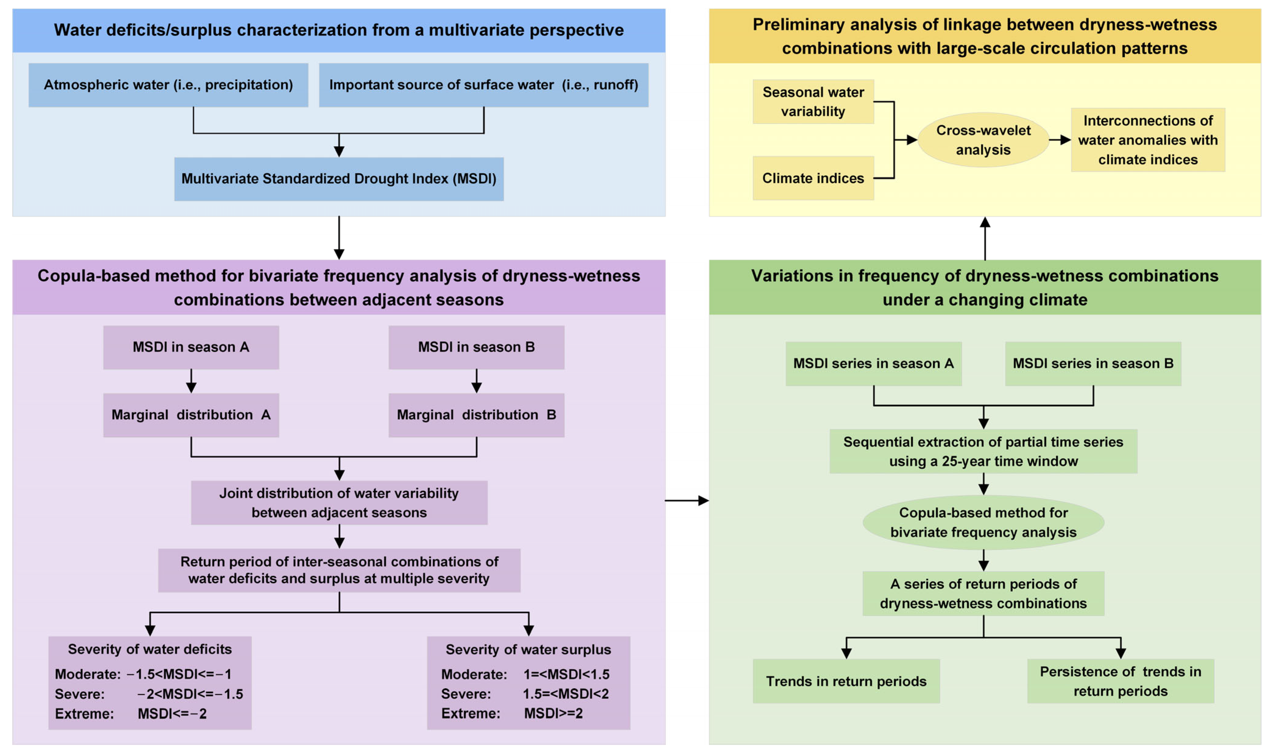
A flowchart as depicted in Figure 2 illustrates how to perform hazard assessment of dryness–wetness combinations between adjacent seasons. Methods utilized are also outlined as follows.

3.1. Multivariate Standardized Drought Index (MSDI)

The reliable hazard assessment of dryness–wetness combinations firstly stresses the necessity of the accurate identification of dry and wet spells. Dry and wet conditions actually represent the shortage and surplus of water resources in a generalized sense, which means that water availability from multiple sources ought to be evaluated jointly. It is, therefore, more reasonable to monitor water variations with the consideration of multiple hydro-meteorological variables. To this end, this study utilizes an MSDI incorporating information of atmospheric water (i.e., precipitation) and an important source of surface water (namely, runoff) under a nonparametric framework proposed by Hao and AghaKouchak [23]. Via analogy with the widely used standardized precipitation index (SPI), the developed MSDI can be computed on a variable time scale. The formulation of the nonparametric MSDI is presented as follows.
Initially, precipitation and runoff observations were aggregated on the pre-specified time scale (also termed the accumulative period) of interest to yield their composites to be analyzed. Afterward, the joint non-exceedance probability of pairwise precipitation and runoff composites was used as a metric of water variability in a statistical sense, with the probability being close to zero indicating water deficits and the probability approaching one representing water surplus. If one assumes random variables P and R to be the precipitation and runoff composites, the joint non-exceedance probability of concern can be described as Equation (1).
Pr P p k , R r k = F p k , r k
To decrease the computational burden, herein the nonparametric Gringorten plotting position formula is adopted for the calculation of the empirical joint non-exceedance probability. The Gringorten formula is expressed as
Pr P p k , R r k m k 0.44 n + 0.12
where n is the total number of pairwise precipitation–runoff composites and m k denotes the number of paired composites concurrently satisfying conditions of p i p k and r i r k . Finally, the MSDI, as shown in Equation (3), can be derived with the aid of the inverse function of the standard normal distribution. This standardization procedure, in essence, conducts an equiprobability transformation that gives rise to the resultant MSDI value having the same non-exceedance probability as the precipitation–runoff observation under investigation [40].
MSDI k = Φ 1 p k
in which Φ 1 x is the symbol denoting the inverse function of the standard normal distribution.
The MSDI is an integrated index that comprehensively reflects water variability from the perspectives of atmospheric and surface water. Similar to the SPI, positive and negative values inform users of the presence of water surplus and deficits, respectively [41]. Table 1 further elaborates a detailed categorization of dry and wet conditions on the basis of a set of MSDI thresholds.

3.2. Mann–Kendall (MK) Trend Analysis

The MK analysis was conducted to examine the trend against randomness in the MSDI series. The regression coefficient test, Sen’s T test, the MK test, Spearman’s Rho test and covariance analysis [42,43] represent distribution-dependent and distribution-free statistic methods available for trend identification. Distribution-dependent trend detection methods typically with the assumption of the data being normally distributed can be hardly applied to the hydrological time series which are skewed and contain outliers, when any modification is not made. However, the rank-based distribution-free MK analysis has been recommended by the World Meteorological Organization due to its insensitivity to outliers and the robustness against nonlinear trends. A major disadvantage of the MK trend analysis is that the trend may be misinterpreted as a result of the negative influence of autocorrelation in the time series. Correlation analysis revealed that the derived MSDI series were free of autocorrelation, thereby motivating the use of the original MK method for trend detection in this study.
The MK analysis yields a standardized statistic Z for trend identification. The sign of Z signifies the direction of the trend in time series [44]. A positive sign represents an ascending trend and vice versa. In addition, Z is often compared against a standard normal variable Z 1 α / 2 to determine whether the detected trend is significant at the specified significance level α . When the absolute value Z is greater than Z 1 α / 2 , the trend can be classified as being statistically significant. In the study, the 5% significance level was utilized and the corresponding critical value Z 1 α / 2 used for evaluation equaled 1.96. For a more detailed description of the MK method, interested readers can refer to Hamed [45] and Sagarika et al. [44].

3.3. Copula-Based Method for Hazard Assessment of Dryness–Wetness Combinations

Hazard assessment of dryness–wetness combinations mainly followed the sequence of fitting the marginal distribution to seasonal water variability (quantified by the MSDI), modeling the joint distribution of water changes between adjacent seasons and estimating the frequency of diverse dryness–wetness combinations.

3.3.1. Marginal Distribution

The marginal distribution is the projection of a multivariate joint distribution onto one of its constituent variables. According to the definition in Section 3.1, the MSDI values can theoretically vary from negative to positive infinity. In the study, the normal, logistic, generalized extreme value (GEV) and stable distributions, which are valid for both positive and negative values, were fitted to the derived MSDI series. Parameters of candidate marginals were estimated using the maximum likelihood method. In the further selection of the optimal marginal, the Kolmogorov–Smirnov (K-S) test was initially used to check whether MSDI values could be drawn from candidate marginals. Metrics of the goodness-of-fit including the root mean square error (RMSE) and the Akaike information criterion (AIC) were subsequently calculated through the comparison between theoretical non-exceedance probabilities derived from candidate marginals and empirical non-exceedance probabilities acquired via the Gringorten plotting-position formula as shown in Equation (2). A candidate marginal yielding the smallest values of the RMSE and AIC ultimately qualifies as the optimal one.

3.3.2. Copula Functions for Deriving the Joint Distribution

As water variability within a season is of concern, marginal distributions of the MSDI on a three-month scale were specifically derived for each season by following the procedures proposed in Section 3.3.1. Afterward, marginal distributions of the MDSI between adjacent seasons (spring and summer, for instance) were combined using the copula function to derive joint distribution.
A copula function with its independent variables being uniformly distributed in the interval of [ 0 ,   1 ] is increasingly popular in hydrology, finance [46] and medicine [47] for diverse applications. The use of copulas simplifies the modeling of joint distributions into two steps (i.e., the estimation of marginals and the determination of an appropriate copula function to describe the dependence structure of variables of interest). Sklar’s theorem [48] states that an arbitrary n -dimensional distribution function can be derived by means of the copula function C x as follows:
F x 1 ,   x 2 ,   ,   x n = C F X 1 x 1 , F X 2 x 2 ,   ,   F X n x n
in which F X i x i denotes the cumulative distribution function of a random variable X i .
As shown in Table 2, Gaussian, Clayton, Gumbel and Frank copulas were applied to modeling joint distributions of the MSDI series between adjacent seasons, among which Gumbel and Clayton copulas were favored in describing the upper and lower tail dependence, respectively. The goodness-of-fit of candidate copulas was evaluated using the Cramér–von Mises statistic and the AIC [49], which could be computed using the ‘VineCopula’ package for R environment. Smaller values of the employed metrics indicate higher fitness. Herein presented is merely a brief introduction to the copula theory and more details can be found in Nelsen [50] and Genest and Favre [51].

3.3.3. Joint Return Period

Joint return periods of dryness–wetness combinations between adjacent seasons can be estimated conditioned on the derived joint distribution. Let X and Y denote the MSDI series of two successive seasons. F X x and F Y y are their marginal distributions and the corresponding joint distribution is F X Y x , y . Joint return periods of four types of combinations of dry and wet spells (namely, the continued dryness, the continued wetness, The transition from dryness to wetness and The transition from wetness to dryness) are given by Equations (5)–(8), respectively.
T X < x Y < y = 1 P X < x , Y < y = 1 F X Y x , y
T X > x Y > y = 1 P X > x , Y > y = 1 1 F X x F Y y + F X Y x , y
T X < x Y > y = 1 P X < x , Y > y = 1 F X x F X Y x , y
T X > x Y < y = 1 P X > x , Y < y = 1 F Y y F X Y x , y
In order to present the results of hazard assessment in an elaborated way, return periods were jointly computed for dryness–wetness combinations with three severity levels. The severity of dry and wet conditions was differentiated using a set of the MSDI thresholds (see Table 1). The corresponding formulas are displayed in Table 3.

3.4. Rescaled Range (R/S) Analysis

The Hurst coefficient (also referred to as the Hurst exponent) was used as a metric to quantify the persistence or long-term memory in natural time series. The Hurst coefficient can be estimated through classic R/S analysis, detrended fluctuation analysis, the aggregated variances, wavelet analysis or the semi-variogram [52,53]. Among the diverse approaches available, R/S analysis, first proposed by Hurst [54] in the design of the Aswan Dam, is extensively utilized in fields of hydrology and geophysics due to its robustness and the ease of calculation. Hence, R/S analysis was adopted to assess the persistence of frequency of various dryness–wetness combinations, which possibly arises from a changing climate.
Assume a time series X = x 1 ,   x 2 ,   ,   x n to be analyzed. The mean of the partial time series over the time span τ is calculated as
x τ = 1 τ i = 1 τ x i , τ = 1 ,   2 ,  
Then, the accumulative deviation from the mean is expressed below
X t , τ = i = 1 t x i x τ , 1 t τ
The adjusted range R τ over the time span τ (Equation (11)) is defined, which is the difference between the maximum and the minimum of the accumulative deviation series.
R τ = max X t , τ min X t , τ , 1 t τ
The adjusted range R τ is subsequently standardized by the standard deviation S τ of the partial time series X τ = x 1 ,   x 2 ,   ,   x τ given by Equation (12) to derive the rescaled adjusted range statistic formulated as R τ / S τ . The main finding by Hurst is that for many natural phenomena, R τ / S τ follows the asymptotic law as shown in Equation (13).
S τ = 1 τ i = 1 τ x i x τ 2
R τ / S τ = c τ H
in which H denotes the Hurst coefficient, and c is a constant. To estimate the Hurst coefficient H , Equation (13) is rewritten to yield Equation (14) [55]. Given that the value of R τ / S τ over the contrasting time spans τ is already known, a log–log plot of R τ / S τ against τ can be depicted, in which the slope of the straight line denotes the estimate of H eventually.
log R τ / S τ = H log τ + H log c
The Hurst coefficient with a value greater than 0.5 notifies one that statistical characteristics of time series in the past are likely to persist in the near future. The Hurst coefficient closer to one denotes the increasingly stronger persistence. H = 0.5 means that observations in time series are the result of the Brownian movement and thereby are independent. For a Hurst coefficient smaller than 0.5, statistical characteristics of time series in the near future are opposite to those in the past. The Hurst coefficient increasingly approaching zero indicates the higher probability of the existence of anti-persistence [17].

3.5. Wavelet Analysis

The cross-wavelet transform is applied to investigating linkages between climate signals and variations in dry and wet conditions. The cross-wavelet transform is the extension of the univariate continuous wavelet transform (CWT) in a two-dimensional space. The CWT decomposes a time series in time and frequency domains jointly, dependent on the selected wavelet function. The CWT of a time series ( x t , t = 1 , , n ), in a mathematical sense, is the convolution of x t with a dilated and translated wavelet function, which is expressed as follows:
W t X a , τ = 1 a + x t ψ t τ a d t
in which the asterisk represents the complex conjugate. ψ t τ a is a wavelet function dilated and translated by a and τ , respectively.
Given that complex nonlinear associations tend to extensively exist among hydro-meteorological variables especially in the context of climate change, the classic correlation analysis based on the Pearson or Spearman correlation coefficients, however, is unlikely to capture the potential nonlinearity. To this end, the cross-wavelet transform is brought in towards the proper identification of nonlinear correlation by revealing the common power and relative phase of two series in time–frequency space [56]. Equation (16) provides the mathematical expression of the cross-wavelet transform ( W t X Y a , τ ).
W t X Y a , τ = W t X a , τ W t Y a , τ
where W t X a , τ and W t Y a , τ are separately the CWTs of time series x t and y t , and W t Y a , τ represents the complex conjugate of W t Y a , τ . The argument of the cross-wavelet coefficient W t X Y a , τ indicates the time delay between two series at the time point τ on the scale a . Via analogy to the CWT, the power spectrum of the cross-wavelet transform is calculated as W t X Y a , τ and further represents the strength of dependence. Interested readers are directed to Torrence and Compo [57] for more details.

4. Results

4.1. An Overview of Water Variability in the HRB

The use of the MSDI benefits the reliable monitoring of water deficits and surplus from a multivariate perspective (i.e., the joint consideration of precipitation and runoff anomalies). Trend detection of the MDSI series in an individual month via the MK test further allows one to reveal when the HRB has a trend towards dryness and wetness. A negative value of the MK test statistic Z represents a decreasing trend of the MSDI which is further interpreted as a drying trend, and vice versa. Figure 3 shows the MK test results of the monthly MSDI series in four sub-regions of the HRB over the analysis period 1952–2010.
None of the absolute values of Z being greater than 1.96 reminds one that there exists no ascending or descending trend of the monthly MSDI being statistically significant at the 5% significance level. In detail, it is shown by the negative Z that the MSDI values dominantly exhibit downward trends in March, April, September, October and November, which implies that the HRB has an insignificant trend towards dryness in early and middle spring as well as in the whole of autumn over the past half-century. Statistics indicate that grain yields from the HRB account for over one sixth of the national total. Seed sprouts and crop growth in spring largely determine annual yields in agricultural sectors. The drying trend in early and middle spring, therefore, ought to catch the sufficient attention of decision-makers in order to cope with the increasing water deficits. In contrast, the MSDI values in February, May, June, July and August are generally dominated by upward trends, suggesting the existence of wetting trends in late winter and the flood season. Given that the most precipitation (60–80%) occurs between June and September in the HRB, the wetter flood season stresses the requirement of more efforts to mitigate the adverse influence of possibly intensified floods. It is noted that the dryness and wetness trends detected above are in line with findings by He et al. [58] that there has been a prevailing trend of drying in spring and autumn and wetting in summer during 1961–2013.

4.2. Frequency Analysis of Inter-Seasonal Combinations of Dry and Wet Conditions in the HRB

The MSDI series on a three-month scale was computed to monitor dry and wet conditions in each season. The time spans of spring, summer, autumn and winter are March–May, June–August, September–November and December–the next February, respectively. The return periods of four kinds of inter-seasonal combinations of dry and wet conditions were calculated for hazard assessment using the copula-based method presented in Section 3.3.

4.2.1. The Selection of Suitable Marginal Distributions

Normal, logistic, GEV and stable distributions were fitted to seasonal MSDI series from 1952 to 2010. The determination of suitable marginals relies on the comparison of the fitness regarding four candidate marginals. The results of the goodness-of-fit test are given in Table 4.
In Table 4, the logical variable H being equivalent to zero suggests that the four candidate marginals jointly pass the K-S test, and the null hypothesis that observations are drawn from the hypothesized distribution is accepted. Afterward, supportive evidence was provided by the AIC and RMSE for screening out the optimal marginals. Candidates with the smallest values of AIC and RMSE were identified as the appropriate ones and are highlighted in bold. The results in Table 4 indicate that none of the four marginal distributions can variably outperform their counterparts in terms of goodness-of-fit metrics used in the present study, revealing the potential risk of exclusively applying a designated marginal for fitting the seasonal MSDI series. Therefore, the joint use of multiple candidate marginals and a goodness-of-fit test is considered as a crucial step towards the accurate characterization of the seasonal MSDI series.

4.2.2. The Determination of Appropriate Copulas

After the derivation of univariate probability distributions of the MSDI series in each season, they were joint together using copulas to yield joint distributions of dryness–wetness combinations between adjacent seasons.
Before constructing the joint distribution, it was necessary to analyze the correlation of the MSDI to be combined between two adjacent seasons. The paired adjacent seasons included S–S, S–A, A–W and W–S, illustrated in Table 5 The mean value of the Kendall correlation coefficient of the MSDI between adjacent seasons is 0.2627, −0.0054, −0.4059 and 0.4164, respectively. It can be seen from the table that the MSDI correlation between winter and spring is the strongest, which is followed by autumn and winter.
The determination of appropriate copulas relies on a statistical test based on Rosenblatt’s transform and the AIC estimate. The statistical test gives rise to two goodness-of-fit metrics. One is the Cramér–von Mises statistic ( S n ) measuring the distance between empirical probabilities and theoretical probabilities. The other is the p-value. For the computation of p-values, the parametric bootstrap described by Genest et al. [59] was used. It is observed in Table 6 that p-values of four candidates (Gaussian, Frank, Clayton and Gumbel copulas) are all greater than 0.05, suggesting that these candidate copulas are applicable to modeling joint distributions of dryness–wetness combinations of concern. The AIC is further employed to screen out the appropriate copulas capable of yielding the smallest bias. To this end, copulas with the smallest AIC values are highlighted in bold in Table 6 and are ultimately determined as the most preferred ones. Note that there are some null values in the table. This is because MSDI series between adjacent seasons sometimes exhibit a negative correlation. However, the use of Clayton and Gumbel copulas is limited to exclusively modeling the dependence structure of two random variables which are positively correlated.

4.2.3. Return Periods of Dryness–Wetness Combinations between Adjacent Seasons in the HRB

According to Equations (5)–(8), return periods of dryness–wetness combinations between adjacent seasons can be estimated. Meanwhile, to systematically support the hazard assessment, diverse combinations at moderate, severe and extreme severity levels (see Table 3) were separately considered. The corresponding results are presented in Figure 4. For each pairwise adjacent season, bolded values highlight dryness–wetness combinations with the shortest return period. Additionally, joint return periods were calculated for four sub-basins to notify water managers of the spatial variability across the HRB. It is noticed that under the moderate scenario, nine out of sixteen combinations with the shortest joint return periods are classified as being the continuously dry conditions (represented by the yellow rectangle in the figure). The transition from dryness to wetness (denoted by the green rectangle) emerges as a combination with the shortest joint return periods five times, finally ranking in the second position. Under the severe scenario, out of sixteen combinations having the shortest joint return periods, eight and five come from the continued dryness and the transition from dryness to wetness. Similarly, at the extreme level, these two kinds of combinations make up the half and a quarter of sixteen shortest-return-period combinations, respectively. Therefore, frequency analysis of dryness–wetness combinations under three severity scenarios achieves an agreement that the HRB is subject to the continuously dry conditions with the highest frequency throughout the year. Meanwhile, the transition from the dry condition to the wet condition—the second-ranked frequent combinations—should catch the sufficient attention of decision-makers as well.
When the specific focus shifts to each season pair, it is found that in spring–summer, four sub-basins (i.e., the whole HRB) are jointly characterized by the shortest joint return periods of the continuous dryness. In the subsequent summer–autumn, the upper reaches of the HRB and the Yishusi River basin, which is situated in the western and northern parts of the HRB, are still the most frequently subject to the continuously dry condition (i.e., the yellow rectangle), whereas the most frequent combinations turn into the transition from dryness to wetness (i.e., the green rectangle) in the middle and lower reaches of the HRB, which dominantly cover the central and eastern parts of the HRB. When it comes to autumn–winter, abrupt transitions between dry and wet conditions have shorter joint return periods than continuously dry (wet) conditions in all sub-basins. As for winter–spring, the continued dryness has the shortest return period against other combinations, which is observed in three out of four sub-regions. The exception is that the lower reach of the HRB features the most frequent occurrence of the continuously wet conditions in winter–spring. The identification of frequent dryness–wetness combinations for each season pair may enrich the current water-related hazard atlas and contribute to the development of more integrated mitigation strategies.
The calculation of joint return periods also favors revealing the pathway along which the frequent dryness–wetness combinations evolve within a year. The western and northern portions of the HRB (i.e., the upper reach and the Yishusi River basin) are sequentially characterized, under three severity scenarios, by the frequent occurrence of the continued dryness (in spring–summer and summer–autumn), transitions between the dryness and wetness (in autumn–winter) and the continued dryness/wetness (in winter–spring). In comparison, the intra-annual evolution of frequent dryness–wetness combinations in the southern and central parts of the HRB (namely, the middle and lower reaches) follows the pathway of the continuously dry conditions (in spring–summer), transitions between dry and wet conditions (in summer–autumn and autumn–winter) and the continuously dry/wet conditions (in winter–spring). It is noted that compared with the western and northern proportions, the southern and central HRB is subject to the higher frequency of abrupt transitions in advance (i.e., starting from summer–autumn). This spatial difference can be interpreted by the earlier influence of the Meiyu front upon southern and central parts during the East Asian summer monsoon. The Meiyu front moves forward from south to north and brings heavy precipitation in zonal bands with a southwest–northeast tilt, thus resulting in the early reception of abundant rainfall in the southern and central parts during the monsoon active period [60,61]. As a consequence, the southern and central parts of the HRB are more likely to suffer from the abrupt transition events than the northern and western parts.

4.3. Temporal Evolution of Frequency of Dryness–Wetness Combinations under Climate Change

In order to analyze how the frequency of dryness–wetness combinations varies in a changing climate, temporal trends of joint return periods, as well as their persistence in the near future, were examined by means of the MK test and R/S analysis. Using a 25-year time window to slide from the beginning to the end of the 3-month MSDI series for each season, 34 sets of sub-series can be generated in sequence over the period 1952–2010. For an individual set of MSDI sub-series, a collection of joint return periods, as displayed in Figure 4, was calculated using the copula-based method described in Section 3.3. Hence, the joint return period of each kind of dryness–wetness combination will have 34 values on the time axis, which correspond to different time periods. Trend detection of the joint return period series eventually benefits understanding the changing pattern of the frequency of various dryness–wetness combinations in the context of global warming.
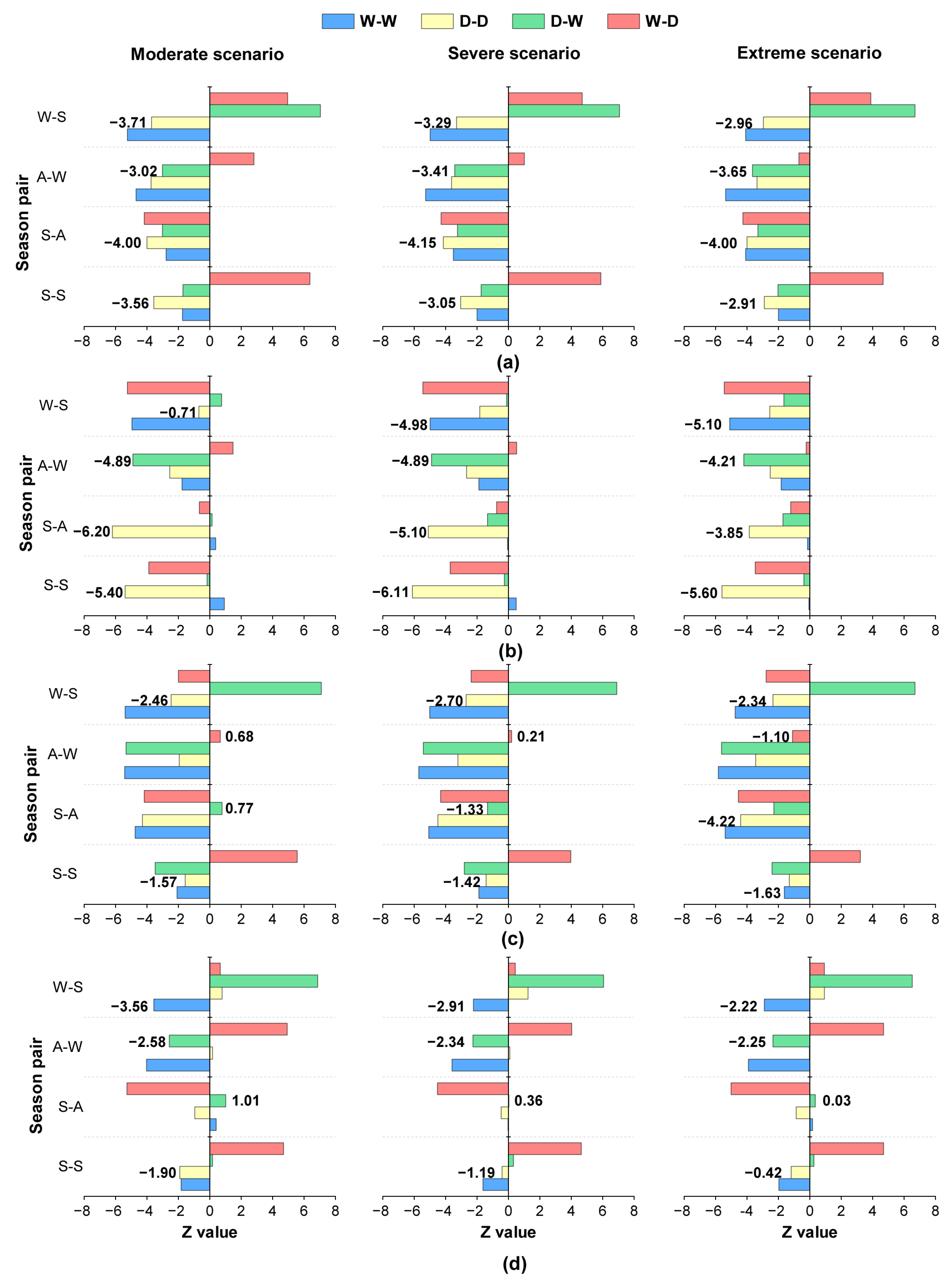
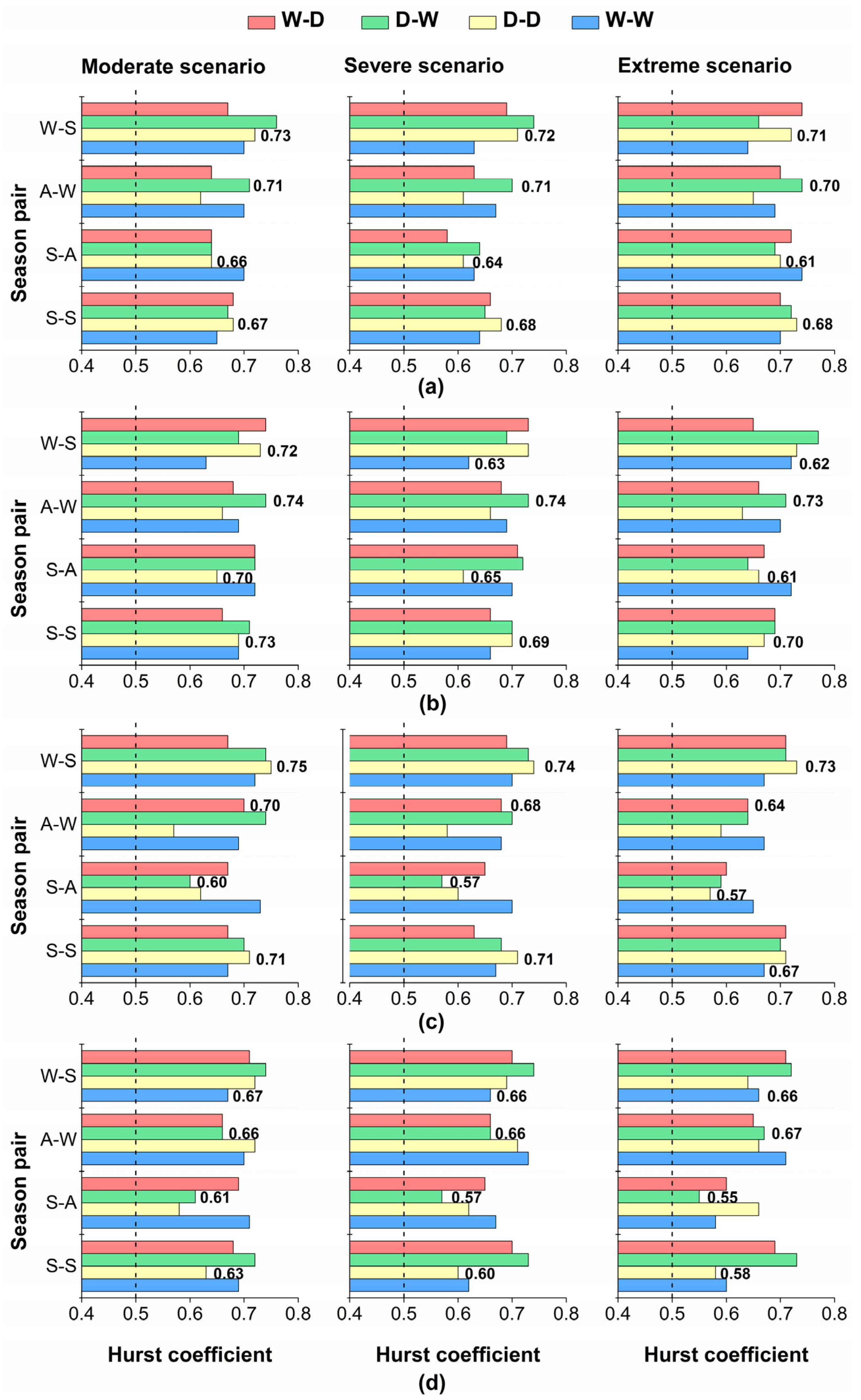
Results regarding trend detection and persistence analysis are presented in Figure 5 and Figure 6 in the form of the MK test statistic Z and the Hurst coefficient, respectively. A negative value of Z means the existence of a decreasing trend in the joint return period of concern, and vice versa. When the Hurst coefficient is greater than 0.5, the detected trend is believed to be persistent in the near future. In Figure 5, 140 out of 192 Z values are negative, indicating that a majority (72.9%) of dryness–wetness combinations had descending return periods during 1952–2010. Moreover, a total of 99 Z values are smaller than −1.96, which corresponds to the critical value at the 5% significance level. This means that more than half (51.5%) of the dryness–wetness combinations have shown significantly downward trends in their return periods. Therefore, the past half-century has generally witnessed the increasingly frequent occurrence of dryness–wetness combinations under three severity scenarios across the entire HRB. In Figure 6, all values of Hurst coefficients exceeding 0.5 further provide supporting evidence that the increasing frequency is likely to persist in the near future. With respect to individual kinds of combinations, 43 out of 48 continuously dry conditions have negative values of Z . The same number is presented by the continuously wet condition. However, a much smaller number of negative Z values is observed in the transition from dryness to wetness or the transition from wetness to dryness, which amounts to being 30 and 24, respectively. As a result, the HRB is more characterized by the widespread intensification of frequency of the continuous dryness/wetness, as compared with the condition in abrupt transitions between dryness and wetness.
As a striking characteristic of the hazard map of the inter-seasonal combinations of dry and wet conditions, the intra-annual evolution pathway of the most frequent combinations invariably catches the attention of decision-makers. In spring–summer, the upper reach of the HRB and the Yishusi River basin are subject to the continuously dry condition with the highest frequency. Z values under three severity scenarios all smaller than −1.96 indicate significant downward trends in the joint return periods of the continuously dry condition, further suggesting the more frequent occurrence of the spring–summer dry condition at the upper reach of the HRB and the Yishusi River basin. Similarly, at the upper reach and the Yishusi River basin, the most frequent dryness–wetness combinations in the following three season pairs (i.e., summer–autumn, autumn–winter and winter–spring) have jointly shown decreasing trends in their joint return periods over the analysis period of 1952–2010. Thereby, the enhanced frequency of the most frequent combinations in each season pair over the past half-century gives rise to a higher possibility of intra-annual evolution of dryness–wetness combinations following the pathway of the prolonged dryness (in spring–summer and summer–autumn), the shift from dryness to wetness (in autumn–winter) and the prolonged dryness/wetness (in winter–spring). When it comes to the middle and lower reaches of the HRB, the return periods of the most frequent dryness–wetness combinations in spring–summer and winter–spring declined during 1952–2010. An earlier analysis of the intra-annual evolution pathway of the frequent combinations confirms that in the remaining season pairs (namely, summer–autumn and autumn–winter), the middle and lower reaches are most frequently hit by transitions between dryness and wetness. However, marked divergence is noted in the changing rates of two types of transition events. In summer–autumn, the transition from wetness to dryness has a trend test statistic (i.e., Z value) towards more negative values than the transition from dryness to wetness, indicating that the frequency of the former transition event escalates much faster than that of the latter. In autumn-winter, the reverse pattern is noticed, whereby the frequency of the transition from dryness to wetness grows at a faster rate. Meanwhile, Hurst exponents greater than 0.5 predict that ascending trends in the frequent dryness–wetness combinations are expected to be persistent in the near future. Therefore, trend detection of joint return periods assists in deducing that the intra-annual evolution of the most frequent dryness–wetness combinations at the middle and lower reaches will be likely to follow an explicit pathway of the continued dryness (in spring–summer), the transition from wetness to dryness (in summer–autumn), the transition from wetness to dryness (in autumn–winter) and the continuous dryness/wetness (in winter–spring) in the future.
Observable ascending or descending trends in joint return periods of other less frequent combinations of interest can be identified as well. The efforts above may lead to a knowledge gain in the dynamic evolution of dryness–wetness combinations in a changing climate.

4.4. Linkages of Climate Indices with Dry and Wet Conditions in the HRB

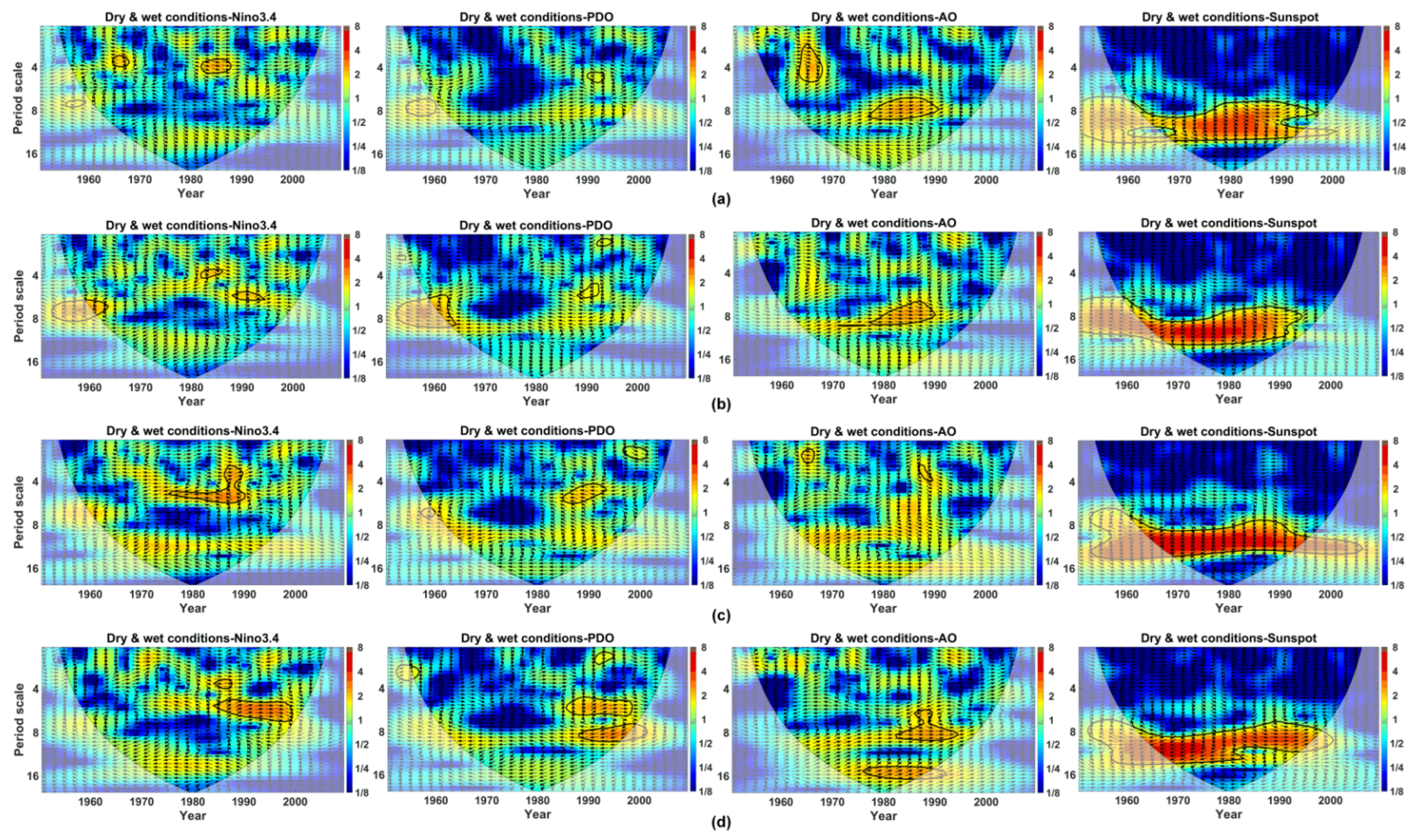
In order to reveal the possible driving forces of water variability in the HRB, its correlations with signals of climate variability are investigated using the cross-wavelet transform in this subsection. The cross-wavelet analysis was conducted based on the annual MSDI series as well as the sunspot number, Nino 3.4 SST, PDO and AO indices during 1952–2010.
The following exclusively exemplifies the results of the cross-wavelet transform at the upper reach of the HRB. It is observed in Figure 7a that the 1964–1968 and 1982–1988 dry and wet conditions are in a significant anti-phase and in-phase relationship with the Nino 3.4 index in the 3–4 years band, respectively. The PDO index is found to be negatively correlated with the 1954–1960 dry and wet conditions on the scale of 7–8 years. Meanwhile, on two scales of 2–5 years and 7–9 years, the AO index shows significantly positive correlations with the regional dryness and wetness. Hence, the intra-decadal oscillation in dry and wet conditions is associated with the PDO, AO and ENSO events. Figure 7a also exhibits the marked linkage between the sunspot number and the 1960–2002 dry and wet conditions in the 8–13 years band. The sunspot number has been widely known to vary with an 11-year solar cycle and exerts influence upon diverse hydro-meteorological processes. As a result, it is reasonable to deduce that sunspot activities have a significant correlation with the near decadal variation in dry and wet conditions at the upper reach of the HRB.
Similar results are also presented in other sub-regions, further providing a reminder that the intra-decadal variation in dry and wet conditions across the HRB is correlated with the PDO, AO and ENSO events. Amongst four types of climate indices investigated here, sunspot activities exert the strongest influences on dry and wet conditions and are likely to be significant forces driving the near decadal oscillation in dry and wet conditions. The findings above may benefit the early warning of dryness–wetness combinations by offering some predictive signals. Merely a preliminary attribution analysis is provided from the perspective of large-scale circulation influence. The physical mechanism underlying the identified linkage, in conjunction with additional factors that may affect water variability in an interactive way, deserves our further investigation.

5. Conclusions

Abrupt transitions from dryness (wetness) to wetness (dryness), though catching less attention, prevail in regions transitioning between humid and arid climates. In comparison with independent water deficits/surplus, the occurrence of abrupt transition events with high severity tends to cost more relief efforts. In order to supplement the current hazard atlas of the water-related hazards, this study, more generally, assesses inter-seasonal combinations of dry and wet conditions (including mutual transitions between dryness and wetness and the prolonged dryness and the prolonged wetness) in the HRB, which is a typical climate transition zone in China. Hazard assessment was performed based on the MSDI over the period 1952–2010. The MSDI joins atmospheric water (i.e., precipitation) and an important source of surface water (namely, runoff), the use of which affords an opportunity to reliably monitor water availability from a multivariate perspective. First, trends in MSDI series were detected by means of the MK test to investigate intra-annual water variability over the past half-century. Afterward, a copula-based method was proposed to estimate the bivariate return periods of dryness–wetness combinations between adjacent seasons under three severity (i.e., moderate, severe and extreme) scenarios. Given that climate warming has resulted in notable tempo-spatial changes in water availability across the globe, the trends and persistence of derived return periods were investigated using a 25-year time window, in order to gain knowledge about the changing pattern of dryness–wetness combinations under a changing climate during 1952–2010. In addition, the cross-wavelet transform was employed to identify the linkage of climate indices with dry and wet conditions in the HRB, which can provide predictive signals for dryness–wetness combinations from the perspective of teleconnection.
Results indicate that the majority of spring and the entirety of autumn have had insignificant trends toward dryness over the past half-century, whilst there is an unremarkably wetting trend in the flood season (June–August). Such changes can possibly intensify flood volume and impose adverse influence on agricultural activities in spring when water is essential to seed sprouts and crop growth. The hazard assessment of dryness–wetness combination under three severity scenarios reveals that, within a year, the HRB is subject to the continued dryness with the highest frequency, which is followed by the abrupt transition from dryness to wetness. Spatially, the southern and central parts of the HRB (also the middle and lower reaches) are more likely to suffer from abrupt transition events than northern and western proportions (also the upper and Yishusi River basin), probably due to the more persistent influence of the Meiyu front on the former parts during the summer monsoon active period. Meanwhile, trend analysis of return periods of dryness–wetness combinations reminds one that under a changing climate, the occurrence of diverse combination events dominantly presents an upward trend across the whole HRB over the past half-century. In particular, the frequency of the continued dryness (wetness) is noted to escalate at a higher rate than that of transition events. Furthermore, preliminary attribution analysis indicates that intra-decadal variations in dry and wet conditions across the HRB are linked to the PDO, AO and ENSO events, and decadal oscillations have a close association with sunspot activities. Hazard assessment in the study improves our understanding of the spatial and temporal preference of dryness–wetness combinations between adjacent seasons, in favor of the enhanced preparedness for water-related hazards.
The increased frequency of dryness–wetness combinations has been widely noted under three severity scenarios in the context of climate change. As the expansion of the current work, our future study will be directed toward the evaluation of their possible implications for agricultural production and water supply, and the development of the relevant adaptation strategies.

Author Contributions

Conceptualization, T.L.; Data curation, L.B.; Formal analysis, G.C.; Funding acquisition, G.C., T.L. and W.F.; Investigation, S.W. and W.F.; Methodology, J.S; Resources, S.W.; Supervision, T.L.; Visualization, J.S.; Writing-original draft, G.C. and W.F. All authors have read and agreed to the published version of the manuscript.

Funding

This research was funded by the Natural Science Foundation of Inner Mongolia (grant number 2021ZD12), Ecological Investigation and Detection of the Second Phase Protection Project in Inner Mongolia Section of Yellow River (grant number RH2000000941), the National Natural Science Foundation of China (grant number 52009100), China Postdoctoral Science Foundation (grant number 2021M692602) and Yinshanbeilu Grassland Eco-hydrology National Observation and Research Station, China Institute of Water Resources and Hydropower Research (grant number YSS2022006).

Institutional Review Board Statement

Not applicable.

Informed Consent Statement

Not applicable.

Data Availability Statement

The data are available from the corresponding author upon request.

Acknowledgments

We want to thank the editor and anonymous reviewers for their valuable comments and suggestions to this paper.

Conflicts of Interest

The authors declare no conflict of interest.

References

  1. Eini, M.; Kaboli, H.S.; Rashidian, M.; Hedayat, H. Hazard and vulnerability in urban flood risk mapping: Machine learning techniques and considering the role of urban districts. Int. J. Disaster Risk Reduct. 2020, 50, 101687. [Google Scholar] [CrossRef]
  2. Lesk, C.; Rowhani, P.; Ramankutty, N. Influence of extreme weather disasters on global crop production. Nature 2016, 529, 84–87. [Google Scholar] [CrossRef] [Green Version]
  3. Nauditt, A.; Stahl, K.; Rodríguez, E.; Birkel, C.; Formiga-Johnsson, R.M.; Kallio, M.; Ribbe, L.; Baez-Villanueva, O.M.; Thurner, J.; Hann, H. Evaluating tropical drought risk by combining open access gridded vulnerability and hazard data products. Sci. Total Environ. 2022, 822, 153493. [Google Scholar] [CrossRef] [PubMed]
  4. Niu, J.; Kang, S.; Zhang, X.; Fu, J. Vulnerability analysis based on drought and vegetation dynamics. Ecol. Indic. 2019, 105, 329–336. [Google Scholar] [CrossRef]
  5. Hu, W.; She, D.; Xia, J.; He, B.; Hu, C. Dominant patterns of dryness/wetness variability in the Huang-Huai-Hai River Basin and its relationship with multiscale climate oscillations. Atmos. Res. 2021, 247, 105148. [Google Scholar] [CrossRef]
  6. Li, X.; Zhang, Q.; Zhang, D.; Ye, X. Investigation of the drought–flood abrupt alternation of streamflow in Poyang Lake catchment during the last 50 years. Hydrol. Res. 2017, 48, 1402–1417. [Google Scholar] [CrossRef]
  7. Yan, D.-H.; Han, D.-M.; Wang, G.; Yuan, Y.; Hu, Y.; Fang, H.-Y. The evolution analysis of flood and drought in Huai River Basin of China based on monthly precipitation characteristics. Nat. Hazards 2014, 73, 849–858. [Google Scholar] [CrossRef]
  8. Banner, J.L.; Jackson, C.S.; Yang, Z.L.; Hayhoe, K.; Woodhouse, C.; Gulden, L.; Jacobs, K.; North, G.; Leung, R.; Washington, W.; et al. Climate change impacts on Texas water a white paper assessment of the past, present and future and recommendations for action. Tex. Water J. 2015, 1, 1–19. [Google Scholar]
  9. Moorhead, J.E.; Gowda, P.H.; Singh, V.P.; Porter, D.O.; Marek, T.H.; Howell, T.A.; Stewart, B. Identifying and Evaluating a Suitable Index for Agricultural Drought Monitoring in the Texas High Plains. JAWRA J. Am. Water Resour. Assoc. 2015, 51, 807–820. [Google Scholar] [CrossRef] [Green Version]
  10. Gu, H.; Yu, Z.; Wang, G.; Wang, J.; Ju, Q.; Yang, C.; Fan, C. Impact of climate change on hydrological extremes in the Yangtze River Basin, China. Stoch. Environ. Res. Risk Assess. 2015, 29, 693–707. [Google Scholar] [CrossRef]
  11. Najafi, M.R.; Moradkhani, H. Multi-model ensemble analysis of runoff extremes for climate change impact assessments. J. Hydrol. 2015, 525, 352–361. [Google Scholar] [CrossRef] [Green Version]
  12. Trenberth, K.E. Changes in precipitation with climate change. Clim. Res. 2011, 47, 123–138. [Google Scholar] [CrossRef] [Green Version]
  13. Wang, S.; Fu, B.J.; Piao, S.L.; Lü, Y.H.; Ciais, P.; Feng, X.M.; Wang, Y.F. Reduced sediment transport in the Yellow River due to anthropogenic changes. Nat. Geosci. 2015, 9, 38–41. [Google Scholar] [CrossRef]
  14. Yang, S.; Wu, B.; Zhang, R.; Zhou, S. Relationship between an abrupt drought-flood transition over mid-low reaches of the Yangtze River in 2011 and the intraseasonal oscillation over mid-high latitudes of East Asia. J. Meteorol. Res. 2013, 27, 129–143. [Google Scholar] [CrossRef]
  15. Ye, J.; He, Y.; Pappenberger, F.; Cloke, H.L.; Manful, D.Y.; Li, Z. Evaluation of ECMWF medium-range ensemble forecasts of precipitation for river basins. Q. J. R. Meteorol. Soc. 2014, 140, 1615–1628. [Google Scholar] [CrossRef] [Green Version]
  16. Lorenzo-Lacruz, J.; Garcia, C.; Morán-Tejeda, E. Groundwater level responses to precipitation variability in Mediterranean insular aquifers. J. Hydrol. 2017, 552, 516–531. [Google Scholar] [CrossRef]
  17. Huang, S.; Huang, Q.; Leng, G.; Chang, J. A Hybrid Index for Characterizing Drought Based on a Nonparametric Kernel Estimator. J. Appl. Meteorol. Clim. 2016, 55, 1377–1389. [Google Scholar] [CrossRef]
  18. Hao, Z.; Singh, V.P. Drought characterization from a multivariate perspective: A review. J. Hydrol. 2015, 527, 668–678. [Google Scholar] [CrossRef]
  19. Fan, J.; Xu, F.; Sun, X.; Dong, W.; Ma, X.; Liu, G.; Cheng, Y.; Wang, H. Construction and Application of Hydrometeorological Comprehensive Drought Index in Weihe River. Atmosphere 2022, 13, 610. [Google Scholar] [CrossRef]
  20. Farahmand, A.; AghaKouchak, A. A generalized framework for deriving nonparametric standardized drought indicators. Adv. Water Resour. 2015, 76, 140–145. [Google Scholar] [CrossRef]
  21. Liu, Y.; Zhu, Y.; Ren, L.; Yong, B.; Singh, V.P.; Yuan, F.; Jiang, S.; Yang, X. On the mechanisms of two composite methods for construction of multivariate drought indices. Sci. Total. Environ. 2019, 647, 981–991. [Google Scholar] [CrossRef]
  22. Rajsekhar, D.; Singh, V.P.; Mishra, A.K. Multivariate drought index: An information theory based approach for integrated drought assessment. J. Hydrol. 2015, 526, 164–182. [Google Scholar] [CrossRef]
  23. Hao, Z.; AghaKouchak, A. A Nonparametric Multivariate Multi-Index Drought Monitoring Framework. J. Hydrometeorol. 2014, 15, 89–101. [Google Scholar] [CrossRef]
  24. Fan, Y.; Huang, G.; Baetz, B.; Li, Y.; Huang, K. Development of a Copula-based Particle Filter (CopPF) Approach for Hydrologic Data Assimilation under Consideration of Parameter Interdependence. Water Resour. Res. 2007, 53, 4850–4875. [Google Scholar] [CrossRef] [Green Version]
  25. Prairie, J.; Rajagopalan, B.; Lall, U.; Fulp, T. A stochastic nonparametric technique for space-time disaggregation of streamflows. Water Resour. Res. 2007, 43, W03432. [Google Scholar] [CrossRef] [Green Version]
  26. Scott, D.W. Multivariate Density Estimation: Theory, Practice, and Visualization; John Wiley & Sons: Hoboken, NJ, USA, 2015. [Google Scholar]
  27. Zhou, X.; Huang, G.; Wang, X.; Fan, Y.; Cheng, G. A coupled dynamical-copula downscaling approach for temperature projections over the Canadian Prairies. Clim. Dyn. 2017, 51, 2413–2431. [Google Scholar] [CrossRef]
  28. Lai, C.D.; Balakrishnan, N. Continuous Bivariate Distributions; Springer: New York, NY, USA, 2009. [Google Scholar] [CrossRef]
  29. Huang, S.; Li, P.; Huang, Q.; Leng, G. Copula-based identification of the non-stationarity of the relation between runoff and sediment load. Int. J. Sediment Res. 2017, 32, 221–230. [Google Scholar] [CrossRef]
  30. Li, J.; Lei, Y.; Tan, S.; Bell, C.D.; Engel, B.A.; Wang, Y. Nonstationary Flood Frequency Analysis for Annual Flood Peak and Volume Series in Both Univariate and Bivariate Domain. Water Resour. Manag. 2018, 32, 4239–4252. [Google Scholar] [CrossRef]
  31. Sraj, M.; Bezak, N.; Brilly, M. Bivariate flood frequency analysis using the copula function: A case study of the Litija station on the Sava River. Hydrol. Process. 2015, 29, 225–238. [Google Scholar] [CrossRef]
  32. Zong, H.; Bueh, C.; Chen, L.; Ji, L.; Wei, J. A Typical Mode of Seasonal Circulation Transition: A Climatic View of the Abrupt Transition from Drought to Flood over the Middle and Lower Reaches of the Yangtze River Valley in the Late Spring and Early Summer of 2011. Atmos. Ocean. Sci. Lett. 2012, 5, 349–354. [Google Scholar]
  33. Wu, Z.; Li, J.; He, J.; Jiang, Z. Large-scale atmospheric singularities and summer long-cycle droughts-floods abrupt alternation in the middle and lower reaches of the Yangtze River. Chin. Sci. Bull. 2006, 51, 2027–2034. [Google Scholar] [CrossRef]
  34. Nan, S.; Li, J. The relationship between the summer precipitation in the Yangtze River valley and the boreal spring Southern Hemisphere annular mode. Geophys. Res. Lett. 2003, 30, 2262. [Google Scholar] [CrossRef]
  35. Dai, A. Drought under global warming: A review. Wiley Interdiscip. Rev. Clim. Chang. 2011, 2, 45–65. [Google Scholar] [CrossRef] [Green Version]
  36. Najibi, N.; Devineni, N.; Lu, M. Hydroclimate drivers and atmospheric teleconnections of long duration floods: An application to large reservoirs in the Missouri River Basin. Adv. Water Resour. 2017, 100, 153–167. [Google Scholar] [CrossRef] [Green Version]
  37. Li, J.Z.; Wang, Y.X.; Li, S.F.; Hu, R. A Nonstationary Standardized Precipitation Index incorporating climate indices as covariates. J. Geophys. Res. Atmos. 2015, 120, 12–082. [Google Scholar] [CrossRef] [Green Version]
  38. Chen, Y.; Niu, J.; Kang, S.; Zhang, X. Effects of irrigation on water and energy balances in the Heihe River basin using VIC model under different irrigation scenarios. Sci. Total Environ. 2018, 645, 1183–1193. [Google Scholar] [CrossRef]
  39. Liang, X.; Lettenmaier, D.P.; Wood, E.F.; Burges, S.J. A simple hydrologically based model of land surface water and energy fluxes for general circulation models. J. Geophys. Res. Atmos. 1994, 99, 14415–14428. [Google Scholar] [CrossRef]
  40. Liu, Y.; Ren, L.; Hong, Y.; Zhu, Y.; Yang, X.; Yuan, F.; Jiang, S. Sensitivity analysis of standardization procedures in drought indices to varied input data selections. J. Hydrol. 2016, 538, 817–830. [Google Scholar] [CrossRef]
  41. Rad, A.M.; Ghahraman, B.; Khalili, D.; Ghahremani, Z.; Ardakani, S.A. Integrated meteorological and hydrological drought model: A management tool for proactive water resources planning of semi-arid regions. Adv. Water Resour. 2017, 107, 336–353. [Google Scholar] [CrossRef]
  42. Hamed, K.H.; Rao, A.R. A modified Mann-Kendall trend test for autocorrelated data. J. Hydrol. 1998, 204, 182–196. [Google Scholar] [CrossRef]
  43. Kisi, O.; Ay, M. Comparison of Mann–Kendall and innovative trend method for water quality parameters of the Kizilirmak River, Turkey. J. Hydrol. 2014, 513, 362–375. [Google Scholar] [CrossRef]
  44. Sagarika, S.; Kalra, A.; Ahmad, S. Evaluating the effect of persistence on long-term trends and analyzing step changes in streamflows of the continental United States. J. Hydrol. 2014, 517, 36–53. [Google Scholar] [CrossRef]
  45. Hamed, K.H. Trend detection in hydrologic data: The Mann–Kendall trend test under the scaling hypothesis. J. Hydrol. 2008, 349, 350–363. [Google Scholar] [CrossRef]
  46. Cherubini, U.; Gobbi, F.; Mulinacci, S.; Romagnoli, S. Dynamic Copula Methods in Finance; John Wiley & Sons: Hoboken, NJ, USA, 2011. [Google Scholar] [CrossRef]
  47. Emura, T.; Matsui, S.; Rondeau, V. Survival Analysis with Correlated Endpoints: Joint Frailty-Copula Models; Springer: Singapore, 2019. [Google Scholar]
  48. Durante, F.; Fernández-Sánchez, J.; Sempi, C. Sklar’s theorem obtained via regularization techniques. Nonlinear Anal. Theory Methods Appl. 2012, 75, 769–774. [Google Scholar] [CrossRef]
  49. Genest, C.; Rémillard, B.; Beaudoin, D. Goodness-of-fit tests for copulas: A review and a power study. Insur. Math. Econ. 2009, 44, 199–213. [Google Scholar] [CrossRef]
  50. Nelsen, R.B. An Introduction to Copulas; Springer Science & Business Media: Berlin/Heidelberg, Germany, 2007. [Google Scholar]
  51. Genest, C.; Favre, A.-C. Everything You Always Wanted to Know about Copula Modeling but Were Afraid to Ask. J. Hydrol. Eng. 2007, 12, 347–368. [Google Scholar] [CrossRef]
  52. Chamoli, A.; Bansal, A.R.; Dimri, V. Wavelet and rescaled range approach for the Hurst coefficient for short and long time series. Comput. Geosci. 2007, 33, 83–93. [Google Scholar] [CrossRef]
  53. Robinson, P.M. Gaussian Semiparametric Estimation of Long Range Dependence. Ann. Stat. 1995, 23, 1630–1661. [Google Scholar] [CrossRef]
  54. Hurst, H.E. Long-Term Storage Capacity of Reservoirs. Trans. Am. Soc. Civ. Eng. 1951, 116, 770–808. [Google Scholar] [CrossRef]
  55. Matos, J.O.; de Moura, E.P.; Krüger, S.E.; Rebello, J.A. Rescaled range analysis and detrended fluctuation analysis study of cast irons ultrasonic backscattered signals. Chaos Solitons Fractals 2004, 19, 55–60. [Google Scholar] [CrossRef]
  56. Grinsted, A.; Moore, J.C.; Jevrejeva, S. Application of the cross wavelet transform and wavelet coherence to geophysical time series. Nonlinear Process. Geophys. 2004, 11, 561–566. [Google Scholar] [CrossRef]
  57. Torrence, C.; Compo, G.P. A practical guide to wavelet analysis. Bull. Am. Meteorol. Soc. 1998, 79, 61–78. [Google Scholar] [CrossRef]
  58. He, Y.; Ye, J.; Yang, X. Analysis of the spatio-temporal patterns of dry and wet conditions in the Huai River Basin using the standardized precipitation index. Atmos. Res. 2015, 166, 120–128. [Google Scholar] [CrossRef] [Green Version]
  59. Genest, C.; Quessy, J.-F.; Remillard, B. Goodness-of-fit Procedures for Copula Models Based on the Probability Integral Transformation. Scand. J. Stat. 2006, 33, 337–366. [Google Scholar] [CrossRef]
  60. Day, J.A.; Fung, I.; Liu, W. Changing character of rainfall in eastern China, 1951–2007. Proc. Natl. Acad. Sci. USA 2018, 115, 2016–2021. [Google Scholar] [CrossRef] [Green Version]
  61. Luo, Y.; Wang, H.; Zhang, R.; Qian, W.; Luo, Z. Comparison of Rainfall Characteristics and Convective Properties of Monsoon Precipitation Systems over South China and the Yangtze and Huai River Basin. J. Clim. 2013, 26, 110–132. [Google Scholar] [CrossRef] [Green Version]
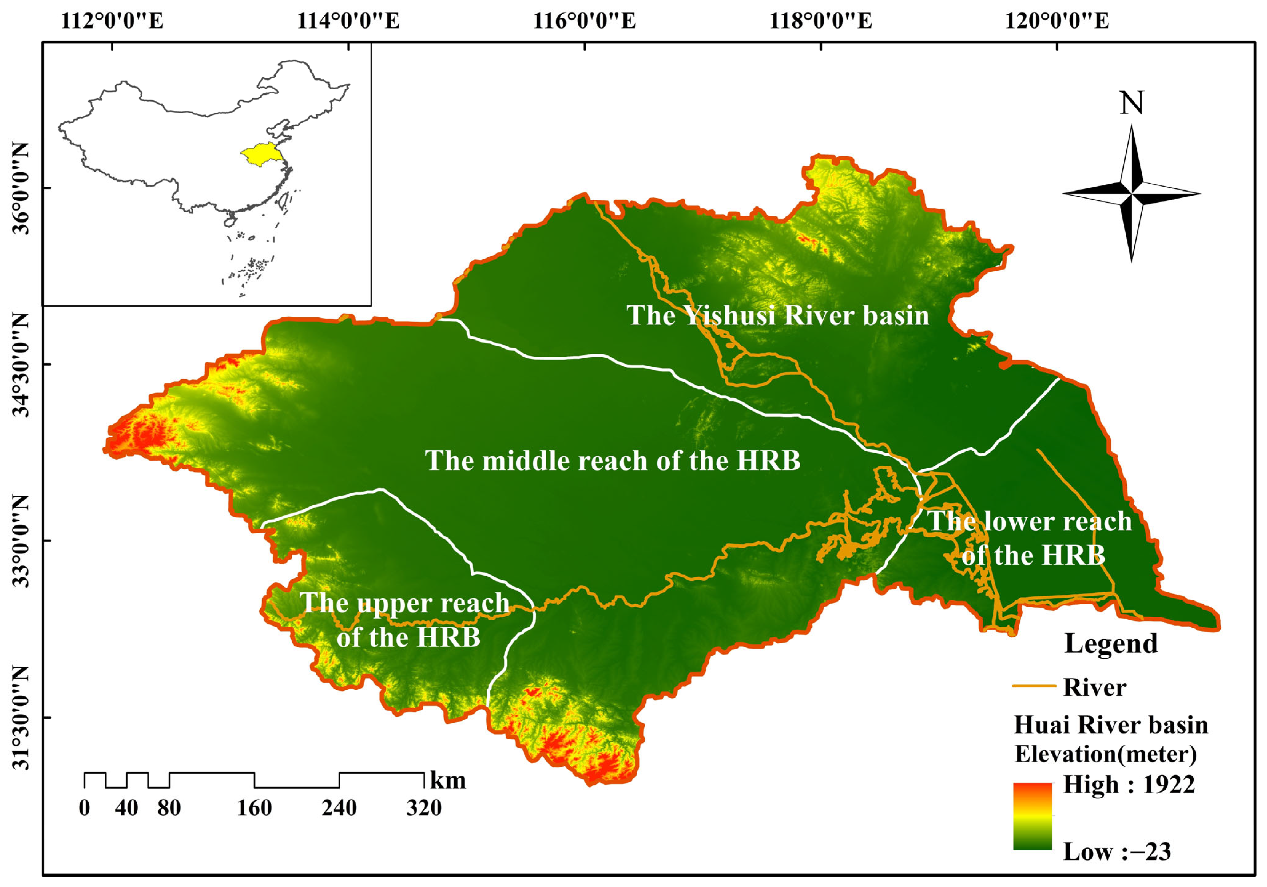
Figure 1. The location and elevation map of the Huai River basin.
Atmosphere 14 00437 g001
Figure 2. A flowchart illustrating procedures for hazard assessment of dryness–wetness combinations between adjacent seasons.
Atmosphere 14 00437 g002
Figure 3. MK test results of monthly MSDI series in four sub-regions of the HRB.
Atmosphere 14 00437 g003
Figure 4. Joint return periods of dryness–wetness combinations between adjacent seasons under three severity scenarios at (a) the upper reach, (b) the Yishusi River basin, (c) the middle reach and (d) the lower reach of the HRB. D–D (W–W) represents a continuously dry (wet) condition between adjacent seasons. D–W (W–D) denotes an abrupt transition from dryness (wetness) to wetness (dryness). Pairwise adjacent seasons include S–S, S–A, A–W and W–S, which are abbreviations for spring–summer, summer–autumn, autumn–winter and winter–spring, respectively.
Atmosphere 14 00437 g004
Figure 5. Trend detection of joint return periods of dryness–wetness combinations under three severity scenarios over the past half-century at (a) the upper reach, (b) the Yishusi River basin, (c) the middle reach and (d) the lower reach of the HRB. Results are presented in the form of the MK test statistic Z . Z values in bold correspond to the most frequent combinations identified for each season pair.
Atmosphere 14 00437 g005
Figure 6. Persistence of trends in return periods of dryness–wetness combinations under three severity level scenarios over the past half-century at (a) the upper reach, (b) the Yishusi River basin, (c) the middle reach and (d) the lower reach of the HRB. Results of persistence analysis are presented in the form of the Hurst coefficient. Values in bold correspond to the most frequent combinations identified for each season pair.
Atmosphere 14 00437 g006
Figure 7. Cross-wavelet transforms between climate indices and the MSDI series at (a) the upper reach of the HRB, (b) the Yishusi River basin, (c) the middle reach of the HRB and (d) the lower reach of the HRB. Thick contours enclose the power spectra of the cross-wavelet transform which are significant against the red noise at the 5% significance level. The lighter shade indicates the cone of the influence where the boundary effect cannot be neglected.
Atmosphere 14 00437 g007
Table 1. The categorization of dry and wet conditions based on the MSDI thresholds.
CategorizationMSDI ThresholdsOccurrence Probability
Extremely wetMSDI ≥ 22.3%
Severely wet1.5 ≤ MSDI < 24.4%
Moderately wet1 ≤ MSDI < 1.59.2%
Nearly normal−1 < MSDI < 168.2%
Moderately dry−1.5 < MSDI ≤ −19.2%
Severely dry−2 < MSDI ≤ −1.54.4%
Extremely dryMSDI ≤ −22.3%
Table 2. The description of candidate copulas.
NameExpressionParameter RangeGeneratorKendall’s Tau
Gaussian Φ ρ Φ 1 u , Φ 1 v ρ 1 ,   1 / 2 arcsin ρ π
Frank 1 θ ln 1 + exp θ u 1 exp θ v 1 exp θ 1 θ ,   \ 0 ln exp θ t 1 exp θ 1 1 + 4 D 1 θ 1 θ
Gumbel exp ln u θ + ln v θ 1 / θ θ 1 ,   ln t θ 1 1 θ
Clayton max u θ + v θ 1 1 / θ , 0 θ 1 ,   \ 0 1 θ t θ 1 θ 2 + θ
Table 3. Joint return periods of dryness–wetness combinations under three severity scenarios.
Type of Dryness–Wetness CombinationsModerate ScenarioSevere ScenarioExtreme Scenario
The continued dryness T M D M D = T x < 1 ,   y < 1 T S D S D = T x < 1.5 ,   y < 1.5 T E D E D = T x < 2 ,   y < 2
The continued wetness T M W M W = T x > 1 ,   y > 1 T S W S W = T x > 1.5 ,   y > 1.5 T E W E W = T x > 2 ,   y > 2
The transition from dryness to wetness T M D M W = T x < 1 ,   y > 1 T S D S W = T x < 1.5 ,   y > 1.5 T E D E W = T x < 2 ,   y > 2
The transition from wetness to dryness T M W M D = T x > 1 ,   y < 1 T S W S D = T x > 1.5 ,   y < 1.5 T E W E D = T x > 2 ,   y < 2
Table 4. The goodness-of-fit of four candidate marginals.
Sub-BasinSeasonNormalLogisticGEVStable
HPRMSEAICHPRMSEAICHPRMSEAICHPRMSEAIC
The upper reach
of the HRB
Sp00.990.01−484.2900.960.02−450.4801.000.01−492.9800.990.01−480.31
Su00.980.02−462.8200.990.02−464.6401.000.02−470.0900.980.02−458.77
A00.920.02−464.8800.990.02−458.2500.820.02−450.8100.920.02−460.86
W01.000.02−475.5100.980.02−456.8401.000.02−472.5701.000.02−471.51
The Yishusi
River basin
Sp00.870.02−437.0000.810.03−414.8800.950.02−450.4300.870.02−433.02
Su01.000.02−466.3800.990.02−438.3501.000.02−476.9001.000.02−462.39
A01.000.02−465.8000.990.02−453.8600.990.02−457.2601.000.02−461.81
W01.000.02−457.5700.990.02−436.6901.000.02−460.5101.000.02−453.57
The middle reach
of the HRB
Sp00.940.02−448.9200.980.02−451.6600.960.02−448.6800.940.02−444.92
Su01.000.02−454.7201.000.02−456.9601.000.02−448.9501.000.02−450.73
A01.000.01−499.7501.000.01−487.9801.000.02−475.4201.000.01−495.76
W01.000.01−490.2601.000.02−477.5401.000.01−499.1201.000.01−486.28
The lower reach
of the HRB
Sp01.000.02−479.2100.990.02−452.7101.000.02−480.5301.000.02−475.19
Su01.000.02−477.1100.980.02−448.4900.990.02−466.8901.000.02−473.11
A01.000.01−494.1600.990.02−457.4601.000.01−496.5601.000.01−490.15
W01.000.01−529.3101.000.01−488.3301.000.01−518.0501.000.01−525.32
Note: Sp, Su, A and W are abbreviations for spring, summer, autumn and winter, respectively. Results of the K-S test are presented in the form of H and P . H = 0 indicates the failure to reject the null hypothesis. H = 1 suggests rejecting the null hypothesis. P is a scalar variable in the range of 0 ,   1 , with a smaller value (usually P 0.05 ) indicating the strong evidence against the null hypothesis. Bolded values of goodness-of-fit metrics highlight the optimal marginal distributions.
Table 5. Kendall’s tau correlation coefficient of the MSDI in adjacent seasons.
Sub-BasinS–SS–AA–WW–S
The upper reach of HRB0.310.24−0.350.46
The Yishusi River basin0.260.27−0.390.49
The middle reach of HRB0.22−0.23−0.500.37
The lower reach of HRB0.26−0.30−0.380.35
Note: pairwise adjacent seasons include S–S, S–A, A–W and W–S, which are abbreviations for spring–summer, summer–autumn, autumn–winter and winter–spring, respectively.
Table 6. The goodness-of-fit of four candidate copulas.
Sub-BasinAdjacent
Seasons
GaussianClaytonGumbelFrank
Snp-ValueAICSnp-ValueAICSnp-ValueAICSnp-ValueAIC
The upper reach
of the HRB
S–S0.080.741.440.080.671.540.080.701.840.080.611.67
S–A0.080.721.960.090.481.990.090.702.000.090.602.00
A–W0.100.551.42//////0.090.651.12
W–S0.190.150.850.220.031.670.180.171.360.090.48−1.77
The Yishusi
River basin
S–S0.120.361.90//////0.090.632.00
S–A0.090.641.830.090.721.900.110.572.000.100.491.96
A–W0.210.25−1.33//////0.250.08−3.23
W–S0.090.591.630.080.641.770.060.86−0.340.060.810.79
The middle reach
of the HRB
S–S0.090.621.580.090.501.890.100.581.200.100.491.88
S–A0.150.251.97//////0.140.311.78
A–W0.150.430.44//////0.150.290.06
W–S0.090.61−0.600.130.240.830.090.54−0.230.060.80−3.22
The lower reach
of the HRB
S–S0.130.361.280.100.441.360.120.341.360.130.291.96
S–A0.110.521.72//////0.120.411.62
A–W0.080.78−0.96//////0.060.930.36
W–S0.080.720.970.060.880.150.080.64−1.420.090.561.02
Note: Pairwise adjacent seasons include S–S, S–A, A–W and W–S, which are abbreviations for spring–summer, summer–autumn, autumn–winter and winter–spring, respectively. Values of goodness-of-fit metrics are highlighted in bold to highlight the optimal copula functions.
Disclaimer/Publisher’s Note: The statements, opinions and data contained in all publications are solely those of the individual author(s) and contributor(s) and not of MDPI and/or the editor(s). MDPI and/or the editor(s) disclaim responsibility for any injury to people or property resulting from any ideas, methods, instructions or products referred to in the content.