Asymptotic Solutions for Equatorial Waves on Venus

Abstract

The atmosphere of Venus exhibits equatorial planetary-scale waves that are suspected to play an important role in its complex atmospheric circulation. Due to its particularly long sidereal day (243 terrestrial days against 24 h for the Earth), the Venusian waves must be described with the momentum equations for a cyclostrophic regime, but efforts to derive analytical wave solutions have been scarce. Following a classic approach for the terrestrial quasi-geostrophic regime, I present analytical solutions for equatorial waves in the atmosphere of Venus, assuming a single layer of a homogeneous incompressible fluid with a free surface and focusing on two asymptotic cases described by the ratio of their non-dimensional frequency and zonal wavenumber. One of the dispersion relations that has been obtained describes waves on a small spatial scale propagating upstream relative to the zonal flow, which is associated with a Rossby-type wave called “centrifugal”. The solutions for the other asymptotic case were interpreted as inertio-surface waves, which describe planetary-scale waves that can propagate “upstream” and “downstream” relative to the zonal winds and have null group velocity. These new wave solutions stress relevant differences between waves in geostrophic and cyclostrophic regimes and may be applicable to Saturn’s moon, Titan, and Venus-like exoplanets.

1. Introduction

Equatorial waves are a particular type of geophysical fluid wave that manifest with a variety of spatial and temporal scales [1]. They propagate in zonal (eastwards and westwards) and vertical directions and are trapped about the equator with a wave amplitude decaying away from the equatorial region [2,3]. In rotating planets, the Coriolis force changes its sign at the equator, thus allowing waves to become trapped even though the Coriolis force is small in this region (with the geostrophic balance no longer expected consequently). The equatorial waves may exist at any altitude level and cause oscillations in pressure, temperature, and winds, these being large enough to influence a large-scale circulation [1]. In the case of the Earth, the equatorial waves are also excited by energetic weather events, such as by the latent heating of organized tropical convection or by a surge of cold air from the extratropical region. Similar to many meteorologically important atmospheric waves, equatorial waves result from displacements in parcels of air due to the influence of different types of restoring forces such as the buoyancy, the pressure gradient, or the Coriolis forces, with the particularity that these forces tend to act together at the equatorial region giving birth to hybrid or mixed waves. Both Kelvin and Rossby-gravity waves have been identified on Earth’s equatorial region, mainly through their perturbations on the wind and temperature fields but also on the outgoing long-wave radiation or modulating/creating global and mesoscale phenomena such as tropical cyclones [1,4,5,6].

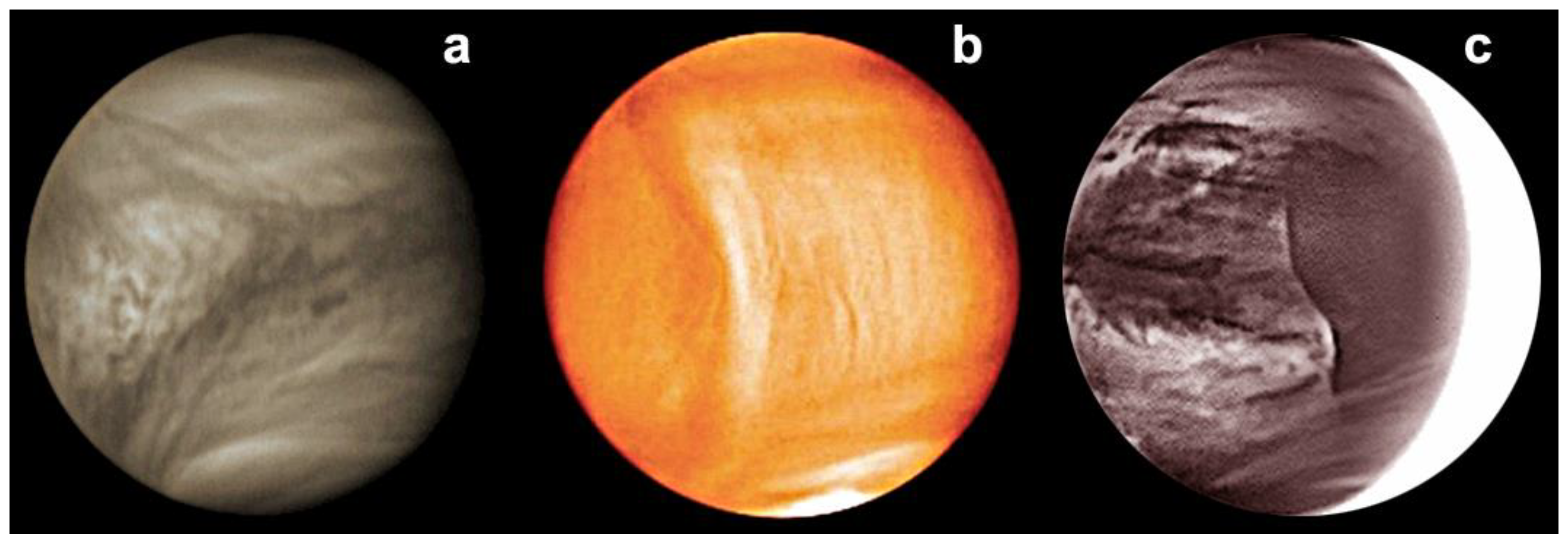
The planet Venus exhibits persistent wave activity in the equatorial region (see Figure 1), as has been repeatedly demonstrated through the analyses of clouds’ albedo, opacity, temperature [7,8,9,10,11,12,13], and wind speeds [10,14,15,16]. Among the global-scale waves that are apparent at the lower latitudes of Venus, the so-called Y structure clearly dominates as a dark horizontal pattern, and during the Pioneer Venus mission, it was reported to rotate with a period of about 4.2 days [7,8], i.e., slower than the prevailing background zonal wind and thus implies an eastward global-scale wave. The Y feature has also been interpreted as a single westward Kelvin wave [10,17,18,19], although reports of other wave modes dominating at mid-latitudes suggest that the Y feature could also be the result of the combined action of two or three waves of different natures such as inertia-gravity, Kelvin, and/or Rossby-Haurwitz waves [7,9,20,21]. An equatorially trapped Kelvin wave seems to be responsible for the recurrent cloud discontinuity recently discovered to propagate along the deeper clouds of Venus, although its physical interpretation is yet an open issue. Therefore, a deeper study of the possible mixed waves that could propagate at the equator of Venus seems required to seek a proper explanation of these phenomena.

In this article, I present an analytical derivation of some wave modes that are possible in the equatorial region of Venus. Towards this aim, I parted from the equations that described a cyclostrophic atmosphere [22,23] and followed a mathematical strategy similar to the classic one used for the Earth’s quasi-geostrophic atmosphere [24]. The work is structured as follows: the general equations for equatorial waves on Venus are presented in Section 2, the generic expressions for the dispersion relations and wave amplitudes are derived in Section 3, the solutions of equatorial waves for two asymptotic cases are obtained, and interpreted in the discussion presented in Section 4, and the conclusions are presented in Section 5.

2. Wave Equations for Equatorial Waves on Venus

Let us assume that the atmosphere of Venus is in cyclostrophic balance can be described as an ideal gas, atmospheric motions are adiabatic, and friction is negligible. After applying a scale analysis that is suitable for Venus, it can be demonstrated [22] that the Venus atmosphere at the cloud region can be described with the following set of equations which include the momentum Equations (1)–(3), the continuity Equation (4), the thermodynamic Equation (5), and the ideal gas Equation (6):

$$\frac{\partial u}{\partial t}+u\frac{\partial u}{\partial x}+v\frac{\partial u}{\partial y}+w\frac{\partial u}{\partial z}=-\frac{1}{\rho }\frac{\partial P}{\partial x}+\frac{uv}{a}\mathit{tan}\varphi$$

(1)

$$\frac{\partial v}{\partial t}+u\frac{\partial v}{\partial x}+v\frac{\partial v}{\partial y}+w\frac{\partial v}{\partial z}=-\frac{1}{\rho }\frac{\partial P}{\partial y}-\frac{u^2}{a}\mathit{tan}\varphi$$

(2)

$$\frac{\partial w}{\partial t}+u\frac{\partial w}{\partial x}+v\frac{\partial w}{\partial y}+w\frac{\partial w}{\partial z}=-\frac{1}{\rho }\frac{\partial P}{\partial z}-g$$

(3)

$$\frac{\partial \rho }{\partial t}+u\frac{\partial \rho }{\partial x}+v\frac{\partial \rho }{\partial y}+w\frac{\partial \rho }{\partial z}=-\rho \left(\frac{\partial u}{\partial x}+\frac{\partial v}{\partial y}+\frac{\partial w}{\partial z}\right)$$

(4)

$$\frac{\partial \Theta }{\partial t}+u\frac{\partial \Theta }{\partial x}+v\frac{\partial \Theta }{\partial y}+w\frac{\partial \Theta }{\partial z}=0$$

(5)

$$P=\rho RT$$

(6)

where $\left(u,v,w\right)$ are the three components of the wind velocity; T, P, and $\rho$ are the atmospheric temperature, pressure, and density; R is the constant for ideal gases; $\Theta$ is the natural logarithm of the potential temperature ($\Theta \equiv \ln \theta$); g is the gravity acceleration on Venus; $z$ is the altitude over the planet surface; $a$ is the Venus radius and $\phi$ is the latitude.

As for equatorial waves on the Earth, we approached our study of equatorial waves using shallow water equations [6,25] with an interface at a certain altitude level ($z=h_0$) and the next disturbances:

$$\begin{array}{ccccc}u& =& u_0& +& u^{\prime }\left(x,y,z,t\right)\\ v& =& & +& v^{\prime }\left(x,y,z,t\right)\\ w& =& & +& w^{\prime }\left(x,y,z,t\right)\\ \rho & =& {\rho }_0\left(z\right)& +& {\rho }^{\prime }\left(x,y,z,t\right)\\ P& =& P_0\left(y,z\right)& +& P^{\prime }\left(x,y,z,t\right)\\ \Theta & =& {\Theta }_0\left(z\right)& +& {\Theta }^{\prime }\left(x,y,z,t\right)\\ h& =& h_0& +& h^{\prime }\left(x,y,z,t\right)\end{array}$$

(7)

where $\left(u^{\prime },v^{\prime },w^{\prime }\right)$ are the wave perturbations for the three components of the wind velocity, ${\rho }_0\left(z\right)$ and $u_0$ are the atmospheric density and zonal wind in their basic states, $P^{\prime },{\rho }^{\prime }$ and ${\Theta }^{\prime }$ are the perturbations for pressure, density, and the natural logarithm of the potential temperature, $h_0$ is the unperturbed height of the interface and $h^{\prime }$ is the perturbation for the vertical level of the interface. As a result, it can be demonstrated that Venus’ atmosphere in the cloud region can be described with the following equations after applying the method of perturbations:

$$\frac{\partial u^{\prime }}{\partial t}+u_0\frac{\partial u^{\prime }}{\partial x}+\frac{\partial }{\partial x}\left(\frac{P^{\prime }}{{\rho }_0}\right)-\Psi \cdot v^{\prime }+\frac{\partial u_0}{\partial y}{v}^{\prime }=0$$

(8)

$$\frac{\partial v^{\prime }}{\partial t}+u_0\frac{\partial v^{\prime }}{\partial x}+\frac{\partial }{\partial y}\left(\frac{P^{\prime }}{{\rho }_0}\right)+2\Psi \cdot u^{\prime }=0$$

(9)

$$n_4\cdot \left(\frac{\partial w^{\prime }}{\partial t}+u_0\frac{\partial w^{\prime }}{\partial x}\right)+\frac{\partial }{\partial z}\left(\frac{P^{\prime }}{{\rho }_0}\right)-n_3\cdot \frac{N^2}{g}\frac{P^{\prime }}{{\rho }_0}-g\cdot {\Theta }^{\prime }=0$$

(10)

$$n_2\cdot \left[\frac{\partial }{\partial t}\left(\frac{{\rho }^{\prime }}{{\rho }_0}\right)+u_0\frac{\partial }{\partial x}\left(\frac{{\rho }^{\prime }}{{\rho }_0}\right)\right]+\frac{\partial u^{\prime }}{\partial x}+\frac{\partial v^{\prime }}{\partial y}+\frac{\partial w^{\prime }}{\partial z}-n_1\cdot \frac{w^{\prime }}{H_0}=0$$

(11)

$$\frac{\partial {\Theta }^{\prime }}{\partial t}+u_0\frac{\partial {\Theta }^{\prime }}{\partial x}+\frac{N^2}{g}\cdot w^{\prime }=0$$

(12)

where $H_0$ is the density scale height (defined as $1/H_0 \equiv -\partial \mathit{ln}{\rho }_0/\partial z$), $N$ is the Brunt–Vaisalla frequency ($N \equiv \sqrt{g\cdot \partial \mathit{ln}\theta /\partial z}$), the term $\Psi \equiv \left(u_0/a\right)\mathit{tan}\phi$ is the centrifugal frequency, and ($n_1, n_2, n_3, n_4$) are tracer parameters that multiply those terms which are key to applying important approximations in the atmosphere and are employed to study the effect of these approximations during a long mathematical derivation [22] (p. 4). In this case, the tracer parameters are linked to the following approximations: the hydrostatic balance ($n_4=0$), incompressible atmosphere ($n_1=n_2=n_3=0$), anelastic atmosphere ($n_2=n_3=0$), and Boussinesq approximation ($n_1=n_2=n_3=n_4=0$) which can be demonstrated to filter out all acoustic waves and part of the gravity waves [22] (p. 10). In addition, since in this work, we are considering that the wave perturbations are not limited to the plane XZ, the perturbed Equations (9)–(11) exhibit an additional term that can be compared with our previous work [22] (p. 4).

To further simplify the equations, we made our next assumptions consistent with studies of terrestrial equatorial waves [24]: (a) waves propagate along the direction west–east with disturbances with the form, $u^{\prime }\left(x,y,z,t\right)=\widehat{u}\left(y,z\right)\cdot \mathit{exp}[i(k_{x}x-\omega t)]$; (b) since we deal with waves in the equatorial region, $\Psi \left(\phi \to 0\right)={\Psi }_0 \cong 0$ [23]; (c) the β-approximation is applicable for the centrifugal frequency $\Psi$ equatorward of 45° [23] (p. 8)—i.e., for a wider meridional extend compared to the Coriolis factor on the Earth—and we can consider that $\Psi$ varies linearly in the meridional direction as $\Psi \approx {\beta }_{\ast } \cdot y$ with ${\beta }_{\ast }<0$ since zonal winds are retrograde on Venus and $u_0<0$ (coefficient ${\beta }_{\ast }$ not to be confused with the coefficient ${\beta }_f$ in the case of the β-approximation for the Coriolis factor); (d) the atmosphere is at rest except for a constant zonal wind $u_0$ [22] (p. 3) and, therefore, we can approximate ${\beta }_{\ast } \approx \frac{u_0}{a^2\cos \phi }$; and, (e) the atmosphere can be regarded as incompressible [26,27], implying that $n_1=n_2=n_3=0$ [22,23]. Therefore, the horizontal momentum Equations (8) and (9) and continuity Equation (11) become:

$$\frac{\partial u^{\prime }}{\partial t}+u_0\frac{\partial u^{\prime }}{\partial x}+\frac{\partial }{\partial x}\left(\frac{P^{\prime }}{{\rho }_0}\right)-{\beta }_{\ast }y \cdot v^{\prime }=0$$

(13)

$$\frac{\partial v^{\prime }}{\partial t}+u_0\frac{\partial v^{\prime }}{\partial x}+\frac{\partial }{\partial y}\left(\frac{P^{\prime }}{{\rho }_0}\right)+2{\beta }_{\ast }y \cdot u^{\prime }=0$$

(14)

$$\frac{\partial }{\partial z}\left(\frac{P^{\prime }}{{\rho }_0}\right)-g \cdot {\Theta }^{\prime }=0$$

(15)

$$\frac{\partial u^{\prime }}{\partial x}+\frac{\partial v^{\prime }}{\partial y}+\frac{\partial w^{\prime }}{\partial z}=0$$

(16)

$$\frac{\partial {\Theta }^{\prime }}{\partial t}+u_0\frac{\partial {\Theta }^{\prime }}{\partial x}+\frac{N^2}{g} \cdot w^{\prime }=0$$

(17)

For shallow water equations, the pressure disturbances can be written in terms of the interface height disturbances [2] (pp. 192–195):

$$\frac{\partial u^{\prime }}{\partial t}+u_0\frac{\partial u^{\prime }}{\partial x}+g\frac{\partial h^{\prime }}{\partial x}-{\beta }_{\ast }y\cdot v^{\prime }=0$$

(18)

$$\frac{\partial v^{\prime }}{\partial t}+u_0\frac{\partial v^{\prime }}{\partial x}+g\frac{\partial h^{\prime }}{\partial y}+2{\beta }_{\ast }y\cdot u^{\prime }=0$$

(19)

$$\frac{\partial h^{\prime }}{\partial z}-{\Theta }^{\prime }=0$$

(20)

$$\frac{\partial u^{\prime }}{\partial x}+\frac{\partial v^{\prime }}{\partial y}+\frac{\partial w^{\prime }}{\partial z}=0$$

(21)

$$\frac{\partial {\Theta }^{\prime }}{\partial t}+u_0\frac{\partial {\Theta }^{\prime }}{\partial x}+\frac{N^2}{g}\cdot w^{\prime }=0$$

(22)

We modified the perturbed continuity Equation (21) in order to express it in terms of interface height disturbances. Since the pressure gradient for shallow water is independent of z, the basic horizontal velocity is also independent of z, i.e., $u\ne u\left(z\right)$ and $v \ne v\left(z\right)$. The unperturbed continuity equation can be vertically integrated from a lower boundary (bottom) to the interface to yield [3] (pp. 192–195):

$$w\left(h_0\right)-w\left(h_{bottom}\right)=-h_e \cdot \left(\frac{\partial u}{\partial x}+\frac{\partial v}{\partial y}\right)$$

(23)

where $h_e=h_0-h_{bottom}$ is known as the equivalent depth, whose only physical significance is that the stratified fluid oscillates in a manner analogous to a homogeneous, incompressible fluid of depth $h_e$ [6,7,9]. In other words, the equivalent depth is the depth of the shallow layer of fluid that is required to give the correct horizontal and time-varying structure of each wave mode [1]. Consequently, for a given atmosphere, there is not a single value for the equivalent depth but as many as possible values for the waves’ phase velocity [28]. Following the classical procedure, we also assumed that for the lower boundary $w\left(h_{bottom}\right)=0$. Thus, w(h₀) was just the rate at which the interface height was changing,

$$w\left(h_0\right)=\frac{Dh}{Dt}=\frac{\partial h}{\partial t}+u\frac{\partial h}{\partial x}$$

(24)

Hence, the vertically integrated continuity Equation (23) can be written:

$$\frac{\partial h}{\partial t}+u\frac{\partial h}{\partial x}+h_e\cdot \left(\frac{\partial u}{\partial x}+\frac{\partial v}{\partial y}\right)=0$$

(25)

which becomes the following after introducing perturbations (7):

$$\frac{\partial h^{\prime }}{\partial t}+u_0\frac{\partial h^{\prime }}{\partial x}+h_e\cdot \left(\frac{\partial u^{\prime }}{\partial x}+\frac{\partial v^{\prime }}{\partial y}\right)=0$$

(26)

Writing the new form of the continuity equation, we have the next set of equations:

$$\frac{\partial u^{\prime }}{\partial t}+u_0\frac{\partial u^{\prime }}{\partial x}+g\frac{\partial h^{\prime }}{\partial x}-{\beta }_{\ast }y \cdot v^{\prime }=0$$

(27)

$$\frac{\partial v^{\prime }}{\partial t}+u_0\frac{\partial v^{\prime }}{\partial x}+g\frac{\partial h^{\prime }}{\partial y}+2{\beta }_{\ast }y \cdot u^{\prime }=0$$

(28)

$$\frac{\partial h^{\prime }}{\partial z}-{\Theta }^{\prime }=0$$

(29)

$$\frac{\partial h^{\prime }}{\partial t}+u_0\frac{\partial h^{\prime }}{\partial x}+h_e\cdot \left(\frac{\partial u^{\prime }}{\partial x}+\frac{\partial v\prime }{\partial y}\right)=0$$

(30)

$$\frac{\partial {\Theta }^{\prime }}{\partial t}+u_0\frac{\partial {\Theta }^{\prime }}{\partial x}+\frac{N^2}{g} \cdot w^{\prime }=0$$

(31)

The disturbances in Equations (27)–(31) can, therefore, be expressed in terms of the wave amplitudes, considering the previous assumption of waves propagating exclusively in the east–west direction, retaining the dependence with y and z for the amplitude, and introducing the intrinsic frequency as $\overline{\omega }=k_x-\omega t$ [22] (p. 4):

$$-i\overline{\omega }\cdot \widehat{u}-{\beta }_{\ast }y \cdot \widehat{v}+i{k}_{x}g \cdot \widehat{h}=0$$

(32)

$$-i\overline{\omega } \cdot \widehat{ v}+2{\beta }_{\ast }y \cdot \widehat{u}+g\frac{\partial \widehat{h}}{\partial y}=0$$

(33)

$$\frac{\partial \widehat{h}}{\partial z}-\widehat{\Theta }=0$$

(34)

$$-i\overline{\omega } \cdot \widehat{h}+i{k}_x{h}_e \cdot \widehat{u}+h_e\frac{\partial \widehat{v}}{\partial y}=0$$

(35)

$$-i\overline{\omega } \cdot \widehat{\Theta }+\frac{N^2}{g} \cdot \widehat{w}=0$$

(36)

Additionally, when combining (34) with (36) we obtain:

$$-i\overline{\omega } \cdot \widehat{u}-{\beta }_{\ast }y \cdot \widehat{v}+i{k}_{x}g \cdot \widehat{h}=0$$

(37)

$$-i\overline{\omega } \cdot \widehat{v}+2{\beta }_{\ast }y \cdot \widehat{u}+g\frac{\partial \widehat{h}}{\partial y}=0$$

(38)

$$\frac{\partial \widehat{h}}{\partial z}+i\frac{N^2}{\overline{\omega }g}\widehat{w}=0$$

(39)

$$-i\overline{\omega } \cdot \widehat{h}+i{k}_x{h}_e \cdot \widehat{u}+h_e\frac{\partial \widehat{v}}{\partial y}=0$$

(40)

3. Dispersion Relation and Wave Amplitude for Equatorial Mixed Waves on Venus

To obtain expressions for the wave amplitude and the dispersion relation for equatorial waves in the cyclostrophic atmosphere of Venus, we combined Equations (37)–(40) to calculate the following quantity $\overline{\omega } \cdot \left(37\right)+k_{x}g \cdot \left(40\right)$:

$$-i{\overline{\omega }}^2 \cdot \widehat{u}-{\beta }_{\ast }y \cdot \overline{\omega } \cdot \widehat{v}+i{k}_x{}^{2}g \cdot h_e\cdot \widehat{u}+k_{x}g \cdot h_e\frac{\partial \widehat{v}}{\partial y}=0$$

(41)

Solving for $\widehat{u}$ and computing $\partial \widehat{u}/\partial y$, we obtained:

$$\widehat{u}=\frac{i}{{\overline{\omega }}^2-k_x{}^{2}g \cdot h_e}\left[\left({\beta }_{\ast }y \cdot \overline{\omega }\right)\cdot \widehat{v}-\left(k_{x}g \cdot h_e\right) \cdot \frac{\partial \widehat{v}}{\partial y}\right]$$

(42)

$$\frac{\partial \widehat{u}}{\partial y}=\frac{i}{{\overline{\omega }}^2-k_x{}^{2}g\cdot h_e}\left({\beta }_{\ast }\overline{\omega }\cdot \widehat{v}+{\beta }_{\ast }y\cdot \overline{\omega }\frac{\partial \widehat{v}}{\partial y}-k_{x}g\cdot h_e\frac{{\partial }^2\widehat{v}}{\partial y^2}\right)$$

(43)

Using Equation (42), we could replace $\widehat{u}$ in (37) to obtain $\widehat{h}$ in terms of solely $\widehat{v}$:

$$\widehat{h}=\frac{i}{{\overline{\omega }}^2-k_x{}^{2}g \cdot h_e}\left[\left(k_x{h}_e{\beta }_{\ast }y\right) \cdot \widehat{v}-\left(\overline{\omega } \cdot h_e\right) \cdot \frac{\partial \widehat{v}}{\partial y}\right]$$

(44)

Considering Equations (42) and (44), it is straightforward to see that at the equatorial region of Venus: (i) waves cannot exist when $\overline{\omega }=\pm \sqrt{h_{e}g} \cdot k_x$, i.e., only waves with a phase speed of $\overline{c_x}\ne \pm \sqrt{h_{e}g}$ are possible, and (ii) the wave disturbances apparent in the zonal velocity and the interface height are both phase-shifted relative to the wave perturbation affecting the meridional velocity.

As a second step, we calculated $\partial /\partial y\left(37\right)-i{k}_x \cdot \left(38\right)$ and replaced the values (42) and (43) to obtain a single equation solely in terms of $\widehat{v}$:

$$(k_x\overline{\omega } \cdot h_{e}g)\frac{{\partial }^2\widehat{v}}{\partial y^2}+({\beta }_{\ast }y \cdot k_x{}^2{h}_{e}g)\frac{\partial \widehat{v}}{\partial y}+({\overline{\omega }}^3{k}_x-\overline{\omega }{k_x}^3{h}_{e}g-{\beta }_{\ast }{k_x}^2{h}_{e}g-2{{\beta }_{\ast }}^2{y}^2{k}_x\overline{\omega })\widehat{v}=0$$

(45)

Rearranging the terms of Equation (45), we could obtain the following second-order differential equation:

$$\frac{{\partial }^2\widehat{v}}{\partial y^2}+\left(\frac{k_x{\beta }_{\ast }}{\overline{\omega }} \cdot y\right) \cdot \frac{\partial \widehat{v}}{\partial y}+\left[\left(\frac{{\overline{\omega }}^2}{h_{e}g}-k_x{}^2-\frac{k_x{\beta }_{\ast }}{\overline{\omega }}\right)-\frac{2{\beta }_{\ast }{}^2}{h_{e}g} \cdot y^2\right] \cdot \widehat{v}=0$$

(46)

which resembles the classic one [1,24] obtained for the geostrophic atmosphere of the Earth (see Equation (47)). In the case of Equation (46), we have a first-order derivative term and variations with latitude, and the centrifugal frequency (${\beta }_{\ast }$) plays a role like that of the Coriolis factor, as can be checked in the following equation derived for the Earth:

$$\frac{{\partial }^2\widehat{v}}{\partial y^2}+\left[\left(\frac{{\omega }^2}{h_{e}g}-k_x{}^2+\frac{k_x{\beta }_f}{\omega }\right)-\frac{{\beta }_f{}^2}{h_{e}g} \cdot y^2\right] \cdot \widehat{v}=0$$

(47)

Since the β-approximation with $\Psi \cong {\beta }_{\ast }y$ has a mostly valid equatorward of 45° [19,23], the solutions must be trapped equatorially to be good approximations of the exact solutions on a sphere [1,3]. For this reason, the disturbances must vanish far away from the equator, i.e., $\widehat{v}\left(\left|y\right|\to \infty \right)=0$. As it was also performed for the terrestrial atmosphere [1], we could simplify the resolution of Equation (46) by using non-dimensional forms for the variables $y, \overline{\omega }\mathrm{and}{k}_x$ via the following changes:

$$y={\rm Y}\cdot {\left(\frac{h_{e}g}{{\beta }_{\ast }{}^2}\right)}^{1/4}\iff \mathsf{{\rm Y}}=y\cdot {\left(\frac{{\beta }_{\ast }{}^2}{h_{e}g}\right)}^{1/4}$$

(48)

$$k_x={\rm K}\cdot {\left(\frac{{\beta }_{\ast }{}^2}{h_{e}g}\right)}^{1/4}\iff \mathsf{{\rm K}}=k_x\cdot {\left(\frac{h_{e}g}{{\beta }_{\ast }{}^2}\right)}^{1/4}$$

(49)

$$\overline{\omega }=\Omega \cdot {\left({\beta }_{\ast }{}^2{h}_{e}g\right)}^{1/4}\iff \mathsf{\Omega }=\overline{\omega }\cdot {\left({\beta }_{\ast }{}^2{h}_{e}g\right)}^{-1/4}$$

(50)

where ${\rm Y}$ is the reduced local meridional coordinate, $K$ is the reduced wavenumber, and $\mathsf{\Omega }$ is the reduced wave frequency. As a result, Equation (46) becomes simplified and adopts the form of the following second-order differential equation:

$$\frac{{\partial }^2\widehat{v}}{\partial {{\rm Y}}^2}+\left(\frac{{\rm K}}{\Omega }\cdot {\rm Y}\right)\cdot \frac{\partial \widehat{v}}{\partial {\rm Y}}+\left[\left({\Omega }^2-{{\rm K}}^2-\frac{{\rm K}}{\Omega }\right)-2{{\rm Y}}^2\right]\cdot \widehat{v}=0$$

(51)

To convert the differential Equation (51) into a second-order differential equation without first derivatives, we assumed that the solution of (51) had the form:

$$\widehat{v}\propto \widehat{A}\left({\rm Y}\right)\cdot \mathit{exp}\left(-\frac{{\rm K}}{4\Omega }\cdot {{\rm Y}}^2\right)$$

(52)

which could then (51) be rewritten as:

$$\frac{{\partial }^2\widehat{A}}{\partial {{\rm Y}}^2}-\left[\left(2+\frac{1}{4}\frac{{{\rm K}}^2}{{\Omega }^2}\right)\cdot {{\rm Y}}^2+\left({{\rm K}}^2-{\Omega }^2+\frac{3}{2}\frac{{\rm K}}{\Omega }\right)\right]\cdot \widehat{A}=0$$

(53)

This equation corresponds to a nonlinear second-order homogeneous differential equation called the Weber equation, whose general expression is [29] (p. 214):

$$\frac{{\partial }^{2}F}{\partial x^2}-\left(a{x}^2+b\right) \cdot F=0$$

(54)

$$\{\begin{array}{c}a=2+\frac{1}{4}\frac{{{\rm K}}^2}{{\Omega }^2}\\ b={{\rm K}}^2-{\Omega }^2+\frac{3}{2}\frac{{\rm K}}{\Omega }\end{array}$$

(55)

Using a simple change in variables, it could be demonstrated [29] (p. 214) that whenever $a>0$, there was an infinite number of solutions n with $b=-\left(2n+1\right) \cdot \sqrt{a},\mathrm{where}n=0,1,2\dots$ and these solutions had the form:

$$F=\mathit{exp}\left(-\frac{\sqrt{a}}{2} \cdot x^2\right) \cdot H_n\left(\sqrt[4]{a} \cdot x\right)$$

(56)

with $H_n\left(z\right)={\left(-1\right)}^n\cdot \mathit{exp}\left(z^2\right)\cdot \frac{d^n}{d{z}^n}\left[\mathit{exp}\left(-z^2\right)\right]$ being the Hermite polynomial of order n. As a result, the wave amplitudes affecting the meridional velocity were:

$${\widehat{v}}_n\left({\rm Y}\right)=\widehat{V}\cdot \mathit{exp}\left[-\frac{1}{2}\left(\sqrt{2+\frac{1}{4}\frac{{{\rm K}}^2}{{\Omega }_n{}^2}}+\frac{{\rm K}}{2{\Omega }_n}\right)\cdot {{\rm Y}}^2\right]\cdot H_n\left(\sqrt[4]{2+\frac{1}{4}\frac{{{\rm K}}^2}{{\Omega }_n{}^2}}\cdot {\rm Y}\right)$$

(57)

where $\widehat{V}$ was the wave amplitude for the meridional velocity when $y=0$, and each solution corresponded to the wave modes $n=0, 1, 2,\dots$ Note that regardless of the sign of the reduced frequency ${\mathsf{\Omega }}_n$, the wave amplitude decayed exponentially as we progressed further away from the equator.

Finally, the dispersion relations for the equatorial waves could be obtained from the following equation:

$${{\rm K}}^2-{\Omega }_n{}^2+\frac{3}{2}\frac{{\rm K}}{{\Omega }_n}=-\left(2n+1\right)\cdot \sqrt{2+\frac{1}{4}\frac{{{\rm K}}^2}{{\Omega }_n{}^2}},\mathrm{where}n=0, 1,2,\dots$$

(58)

4. Discussion

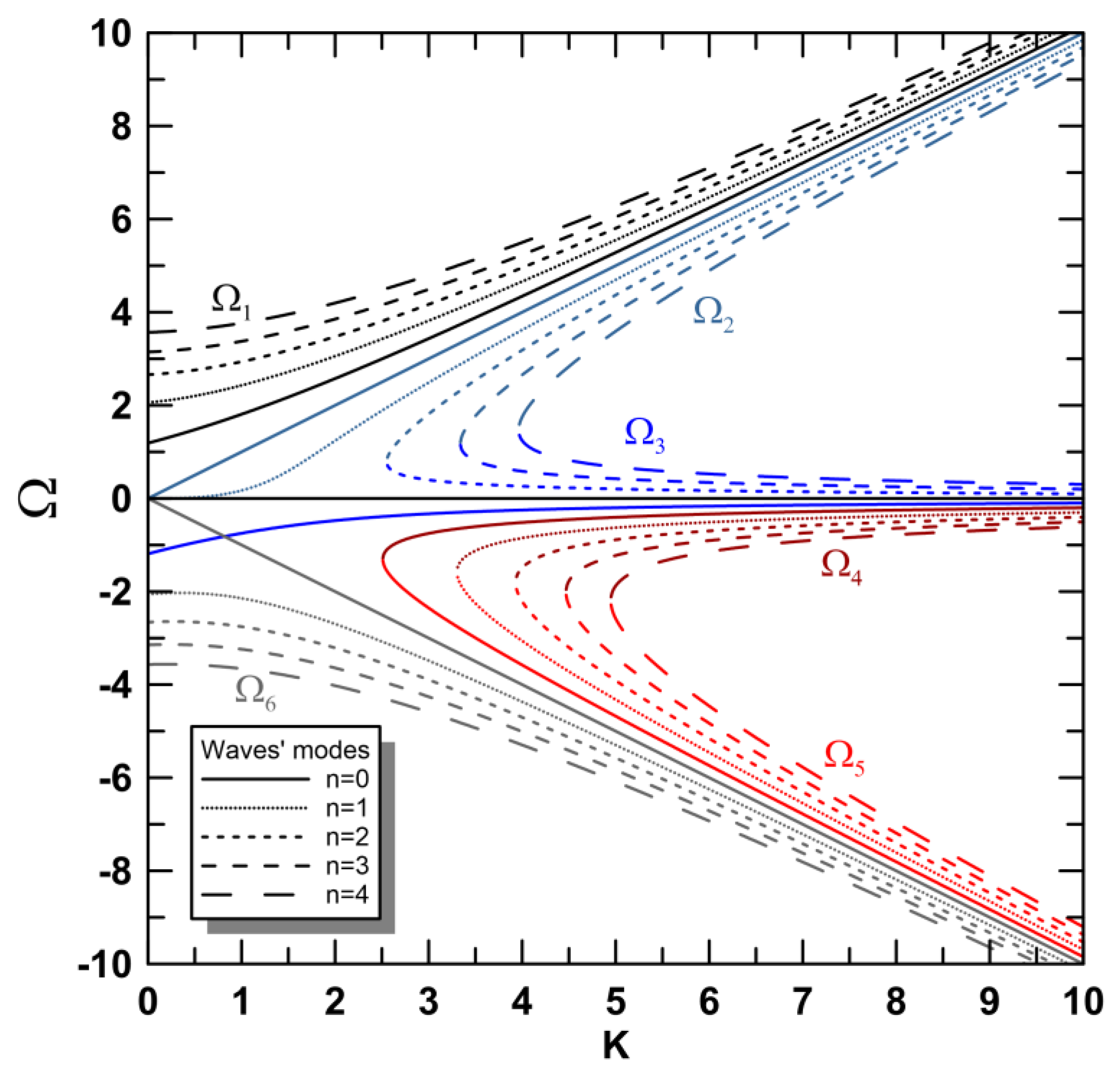
We had to solve Equation (58) for the unknown $\Omega$ in order to obtain a generic expression for the dispersion relation for the equatorial waves on Venus. In contrast with the simpler equation for the geostrophic Earth obtained by Matsuno [24] (p. 28) or Wheeler and Nguyen [1] (p. 103), an exact solution was not possible in this case. Alternatively, we could obtain the roots of Equation (58) numerically if, for each combination of values of the wave mode $n$ and reduced wavenumber $\mathsf{{\rm K}}$, we manipulated (58) to express it as a sextic equation for the unknown $\Omega$:

$$4{\mathsf{\Omega }}^6-8{\mathsf{{\rm K}}}^2{\mathsf{\Omega }}^4-12{\mathsf{{\rm K}}\mathsf{\Omega }}^3+4\left[{\mathsf{{\rm K}}}^2-2{\left(2n+1\right)}^2\right]{\mathsf{\Omega }}^2+12{\mathsf{{\rm K}}}^3\mathsf{\Omega }+{\mathsf{{\rm K}}}^2\left[9-{\left(2n+1\right)}^2\right]=0$$

(59)

Assuming that wave modes with values $n=0,1,2,\dots$ and reduced wavenumbers $\mathsf{{\rm K}}$ have ranging values between ${10}^{-2}$ and ${10}^2$, I calculated the roots for the corresponding sextic equations implementing the Laguerre’s method [30] (pp. 365–368). A total of six roots were obtained, three of them corresponding to waves with $\mathsf{\Omega }>0$ (downstream) and the other three for waves with $\Omega <0$ (see Figure 2).

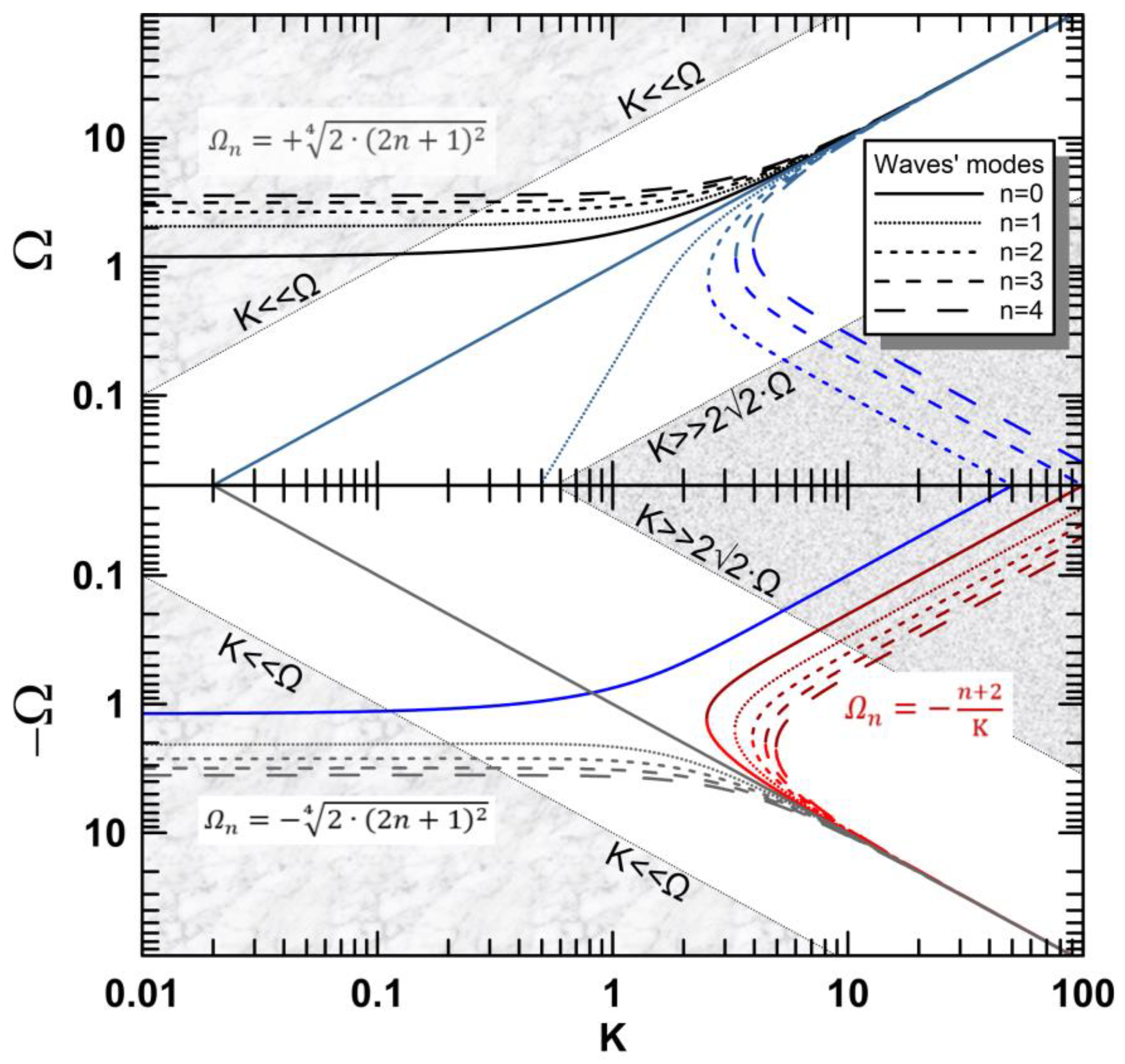
By comparing analogs with the dispersion curves obtained for the atmospheric equatorial waves on the Earth [24] (p. 29), the roots Ω₁ and Ω₆ would correspond to inertio-gravity waves propagating downstream/upstream relative to the mean zonal flow of Venus, while the mode n = 0 of the root Ω₂ might be interpreted as a Kelvin wave which propagates downstream on Venus [19]. On the other hand, the physical interpretation of the other roots is not straightforward. To facilitate the physical interpretation of the equatorial atmospheric waves behind the solutions in Figure 2, I simplified the expressions of dispersion relation (58) and wave amplitude (57) considering two asymptotic cases which considered the argument of the squared roots in (57) and (58): equatorial waves with ${\rm K}/\Omega \gg 2\sqrt{2}$ (or $\left|\overline{c_x}\right|\ll \sqrt{h_{e}g/8}$) and waves with ${\rm K}/\Omega \ll 1$ (or $\left|\overline{c_x}\right|\gg \sqrt{h_{e}g}$). In sub-Section 4.2. it is shown that, in contrast with ${\rm K}/\Omega \ll 2\sqrt{2}$, the asymptotic case ${\rm K}/\Omega \ll 1$ allows an equation to be obtained with which it is easier to solve the dispersion relation.

4.1. Equatorial Waves with ${\rm K}/\Omega \gg 2\sqrt{2}$: Centrifugal Waves

When we have waves fulfilling the condition ${\rm K}/\Omega \gg 2\sqrt{2}$, then ${{\rm K}}^2/{\Omega }^2>>8$, then we also have ${{\rm K}}^2/4{\Omega }^2>>2$ and ${{\rm K}}^2>>{\Omega }^2$. Consequently, the dispersion relation (58) adopts the next simpler form,

$${\Omega }_n=-\frac{n+2}{K}, \mathrm{where} n=0,1,2,\dots$$

(60)

which can describe the root Ω₄ displayed in Figure 2 in the asymptotic area where ${\rm K}/\Omega \gg 2\sqrt{2}$ (see dark red curves in Figure 3).

The dispersion relation (60) can be transformed into dimensioned variables to obtain,

$${\overline{\omega }}_n=-\frac{{\beta }_{\ast }}{k_x}\cdot \left(n+2\right) ,\mathrm{where}n=0, 1,2,\dots$$

(61)

and since on Venus we have ${\beta }_{\ast }<0$ between the equator and midlatitudes [19,23], it is evident that the dispersion relation (61) represents centrifugal waves: a type of Rossby wave that arises as a solution in the cyclostrophic regime of Venus [23] and whose intrinsic frequency is positive $\overline{\omega }>0$ (“upstream” propagation relative to the zonal retrograde flow of Venus, i.e., slower than zonal winds). In fact, the dispersion relation (61) is identical to the limit case of centrifugal waves with short horizontal wavelengths [23] (p. 9) when $n = 0$.

As can be guessed from Figure 3, we can apply again the condition ${\rm K}/\Omega \gg 2\sqrt{2}$ in the dispersion relation (61) to obtain a maximum zonal wavelength:

$${\lambda }_x<<{\left(\frac{{\pi }^2\sqrt{2h_{e}g}}{-{\beta }_{\ast }\cdot \left(n+2\right)}\right)}^{1/2} ,\mathrm{where}n=0, 1,2,\dots$$

(62)

Hence, considering g = 8.87 m s⁻¹, $\left|{\beta }_{\ast }\right| \approx 2\cdot {10}^{-12}{\mathrm{s}}^{-1}{\mathrm{m}}^{-1}$ [19] (pp. 2–3) and an equivalent depth of h_e = 300 m, the maximum zonal wavelength given by (62) barely exceeds ~1300 km in the case of the wave mode $n=0$ (a limit even smaller for higher modes). Therefore, the asymptotic case ${\rm K}/\Omega \gg 2\sqrt{2}$ is not suitable for the description of Rossby-type waves with a planetary spatial scale. This implies an important difference between the theoretical expressions for centrifugal waves on Venus and Rossby waves on Earth since planetary-scale wavelengths are allowed for terrestrial Rossby waves [24] (p. 29). In the case of Venus, only the wave mode n = 0 of the root Ω₃ is consistent with a Rossby-type wave with longer wavelengths (see Figure 2 and Figure 3).

From the dispersion relation (61), we can also deduce expressions for the phase and group speeds:

$${\overline{c_x}}_n=-\frac{{\beta }_{\ast }}{k_x{}^2}\cdot \left(n+2\right),\mathrm{where}n=0, 1,2,\dots$$

(63)

$${\overline{c_g}}_n=\frac{{\beta }_{\ast }}{k_x{}^2}\cdot \left(n+2\right)$$

(64)

whose expressions are very similar to that of centrifugal waves with short horizontal wavelengths [23] (p. 9), with the phase and group velocities demonstrating the opposite sign, while both speeds are faster for higher modes and larger zonal wavelengths.

Concerning the wave amplitude on the meridional velocity (see Equation (57)), this can be also simplified (see Appendix A) to obtain:

$${\widehat{v}}_n\left({\rm Y}\right)=\widehat{V}\cdot \mathit{exp}\left[-\frac{\left|{\Omega }_n\right|}{{\rm K}}\cdot {{\rm Y}}^2\right]\cdot H_n\left(\sqrt{\frac{1}{2}\frac{{\rm K}}{\left|{\Omega }_n\right|}\left(1+\frac{4{\Omega }_n{}^2}{{{\rm K}}^2}\right)}\cdot {\rm Y}\right)$$

(65)

Returning to dimensioned magnitudes, the wave amplitude given by (65) becomes:

$${\widehat{v}}_n\left(y\right)=\widehat{V}\cdot \mathit{exp}\left[-\left|{\beta }_{\ast }\right|\frac{\left|\overline{c_{x,n}}\right|}{h_{e}g}\cdot y^2\right]\cdot H_n\left(\sqrt{\left(\frac{1}{2}\frac{\left|{\beta }_{\ast }\right|}{\left|\overline{c_x}\right|}+2\left|{\beta }_{\ast }\right|\frac{\left|\overline{c_{x,n}}\right|}{h_{e}g}\right)}\cdot y\right)$$

(66)

and using (63), the wave amplitude (65) can be also expressed as,

$${\widehat{v}}_n\left(y\right)=\widehat{V}\cdot \mathit{exp}\left[-\frac{{\beta }_{\ast }{}^2\left(n+2\right)}{k_x{}^2{h}_{e}g}{y}^2\right]\cdot H_n\left(\sqrt{\frac{1}{2}\frac{k_x{}^2}{\left(n+2\right)}+\frac{2{\beta }_{\ast }{}^2}{k_x{}^2{h}_{e}g}\left(n+2\right)}\cdot y\right)$$

(67)

Finally, the meridional e-folding decay width $e^{-y^2/{\sigma }^2}$ is given by the following formula:

$$\sigma =\frac{k_x}{\left|{\beta }_{\ast }\right|}\sqrt{\frac{h_{e}g}{n+2}}=\frac{{\lambda }_x}{2\pi \left|\overline{c_x}\right|}\sqrt{h_{e}g\cdot \left(n+2\right)}$$

(68)

and we used Equation (68) to provide an estimation of the equivalent depth h_e that best described a candidate for centrifugal wave in the observations of Venus, provided that we can measure the intrinsic phase speed in the zonal direction, the horizontal wavelength, and the meridional e-folding decay. Note that since the equivalent depth h_e explicitly appears in Equation (68), this expression cannot be used to predict the meridional e-folding decay width.

4.2. Equatorial Waves with ${\rm K}/\Omega \ll 1$: Inertio-Surface Waves

If we consider the asymptotic case of equatorial waves with ${\rm K}/\Omega \ll 1$, then we also have ${{\rm K}}^2/{\Omega }^2\ll 1$ and, therefore ${{\rm K}}^2/{\Omega }^2\ll 8$. Manipulating (58), we obtain:

$$-{\Omega }^2+\frac{3}{2}\frac{{\rm K}}{\Omega }=-\sqrt{2}\left(2n+1\right)\cdot \sqrt{1+\frac{1}{8}\frac{{{\rm K}}^2}{{\Omega }^2}}$$

(69)

and since ${{\rm K}}^2/8{\Omega }^2\ll 1$, we could approximate $\sqrt{1+X}\underset{X<<1}{\to }1+\left(X/2\right)$ so that:

$$\sqrt{1+\frac{1}{8}\frac{{{\rm K}}^2}{{\Omega }^2}}\approx 1+\frac{1}{16}\frac{{{\rm K}}^2}{{\Omega }^2}$$

(70)

Replacing (70) in (69) and further operating, the equation adopts the form:

$$-{\Omega }^2+\frac{2}{3}\frac{{\rm K}}{\Omega }=-\sqrt{2}(2n+1)\cdot \frac{1}{16}(16+\frac{{{\rm K}}^2}{{\Omega }^2})$$

(71)

Additionally, provided that ${{\rm K}}^2/{\Omega }^2<<8$, it is evident that ${{\rm K}}^2/{\Omega }^2<<16$ and:

$$\frac{2}{3}{\Omega }^2-\frac{{\rm K}}{\Omega }-\frac{2\sqrt{2}}{3}\left(2n+1\right)=0$$

(72)

Provided that ${\rm K}/\Omega \ll 1$, we can further neglect the term ${\rm K}/\Omega$ against the term dependent on (2n + 1) whenever n ≥ 1. Consequently, the dispersion relation (72) adopts the final expression:

$${\Omega }_n=\pm \sqrt[4]{2\cdot {\left(2n+1\right)}^2} ,\mathrm{where}n=1, 2,3,\dots$$

(73)

whose expression in terms of dimensioned variables is:

$${\overline{\omega }}_n=\pm \sqrt[4]{2{{\beta }_{\ast }}^2{h}_{e}g\cdot {\left(2n+1\right)}^2} ,\mathrm{where}n=1, 2,3,\dots$$

(74)

and the wave modes described by the dispersion relations (73) may also be interpreted as inertio-surface waves [23] (p. 6), which can propagate “upstream” or “downstream” relative to the mean zonal flow of Venus. Note that if the wave mode n = 0 exists when ${\rm K}/\Omega \ll 1$, this may not be interpreted as an inertial wave since these are not possible at the equator of Venus [22] (p. 8).

Moreover, using the asymptotic condition ${\rm K}/\Omega \ll 1$, we can set a minimum zonal wavelength for the equatorial waves that can be described with the dispersion relation (74):

$$\lambda x>>{\left(\frac{2{\pi }^2\sqrt{2h_{e}g}}{\left|{\beta }_{\ast }\right|\cdot \left(2n+1\right)}\right)}^{1/2} ,\mathrm{where}n=1, 2,3,\dots$$

(75)

Provided that g = 8.87 m s⁻¹ and $\left|{\beta }_{\ast }\right|\approx 2\cdot {10}^{-12}$ s⁻¹m⁻¹ [19] (pp. 2–3), we needed an equivalent depth as small as h_e = 1 m to obtain a minimum value that would allow waves with zonal wavelengths within the zonal wavenumber one (about 38,500 km in the case of the equator of Venus). Therefore, the asymptotic case ${\rm K}/\Omega \ll 1$ is only appropriate to describe planetary-scale waves, as already observed in the dispersion curves (see Figure 2 and Figure 3). Similar behavior was observed in the case of the inertia-gravity waves for the terrestrial case [24] (p. 29).

These surface waves are demonstrated to have horizontal phase velocities that are faster for higher modes and longer horizontal wavelengths, while their horizontal group velocity is zero:

$${\overline{c_x}}_n=\pm \frac{1}{k_x}\sqrt{{\left(2{\beta }_{\ast }{}^2{h}_{e}g\right)}^{1/2}\cdot \left(2n+1\right)},\mathrm{where}n=1,2,3,\dots$$

(76)

$$\overline{c_{g_n}}=0$$

(77)

With regard to the wave amplitude over the meridional velocity, we could use ${{\rm K}}^2/4{\Omega }^2<<2$ to simplify the wave amplitude (57) to obtain:

$${\widehat{v}}_n\left({\rm Y}\right)=\widehat{V}\cdot \mathit{exp}\left[-\frac{1}{4}\left(2\sqrt{2}+\frac{{\rm K}}{\Omega }\right)\cdot {{\rm Y}}^2\right]\cdot H_n\left(\sqrt[4]{2}\cdot {\rm Y}\right),\mathrm{where}n=0,1,2,\dots$$

(78)

remembering that ${\rm K}/\Omega \ll 2\sqrt{2}$,

$${\widehat{v}}_n\left({\rm Y}\right)=\widehat{V}\cdot \mathit{exp}\left[-\frac{{{\rm Y}}^2}{\sqrt{2}}\right]\cdot H_n\left(\sqrt[4]{2}\cdot {\rm Y}\right),\text{ where }n=0,\text{ 1, 2, }\dots$$

(79)

The dimensioned form for the wave amplitude over the meridional velocity is:

$${\widehat{v}}_n\left(y\right)=\widehat{V}\cdot \mathit{exp}\left[-{\left(\frac{{\beta }_{\ast }{}^2}{2h_{e}g}\right)}^{1/2}{y}^2\right]\cdot H_n\left(\sqrt[4]{\frac{2{\beta }_{\ast }{}^2}{h_{e}g}}\cdot y\right),\mathrm{where}n=0,1,2,\dots$$

(80)

Additionally, there is the fact again that the wave amplitude is modulated in the meridional direction by the product between an e-folding decay and a Hermite polynomial. In the case of the asymptotic case ${\rm K}/\Omega \ll 1$, the meridional e-folding decay width $e^{-y^2/{\sigma }^2}$ is defined by an expression very similar to the e-folding decay obtained for equatorial waves on the Earth [1] (p. 104):

$$\sigma ={\left(\frac{2h_{e}g}{{\beta }_{\ast }{}^2}\right)}^{1/4}$$

(81)

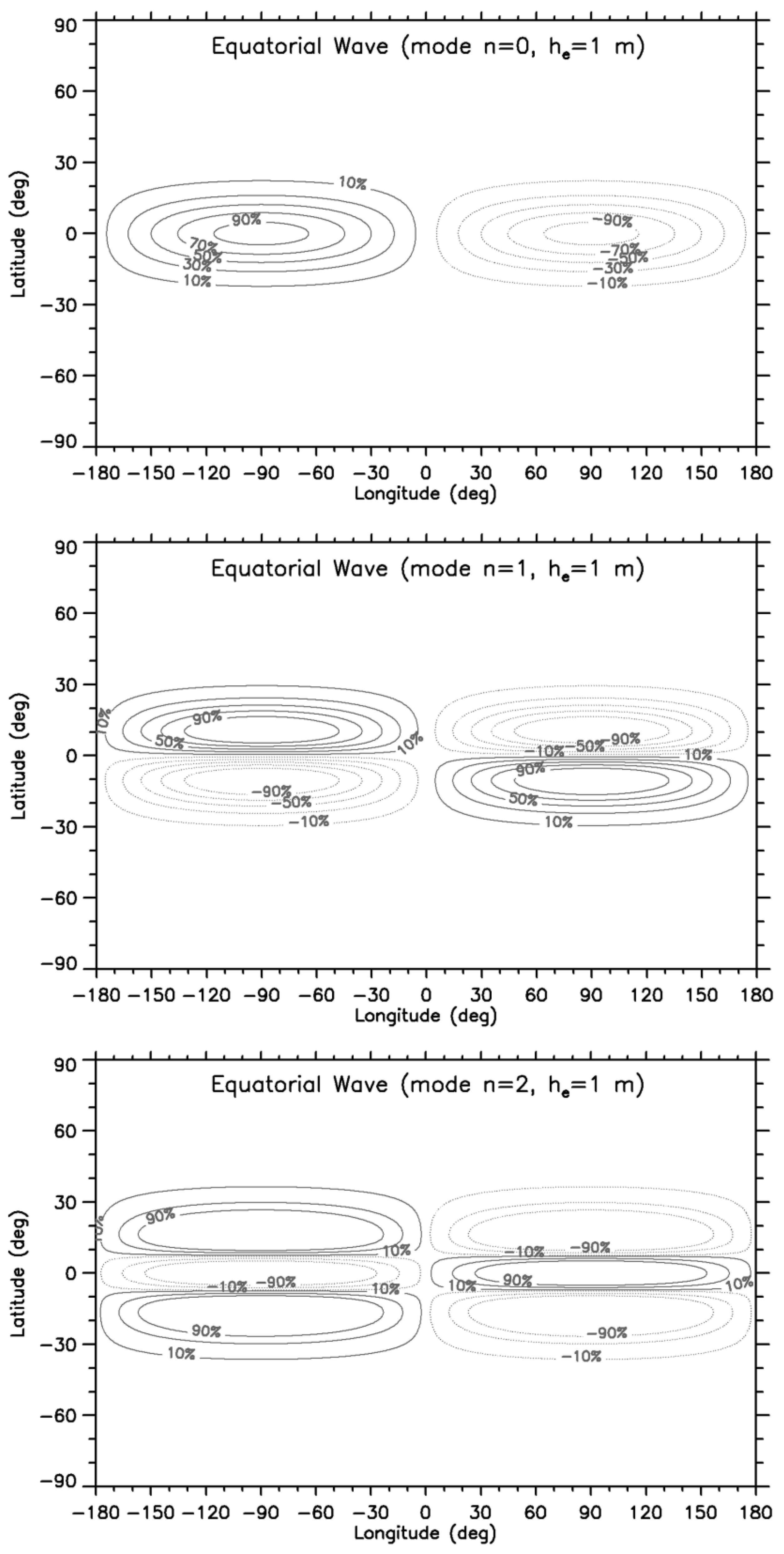
Finally, using the reference model that was used in previous work to study equatorial Kelvin waves on Venus [19], we could use (80) to exhibit the horizontal structure at 70 km above the surface of the first wave modes, considering a zonal wavenumber one and h_e = 1 m (see Figure 4). It can be checked that for wave modes $n\ge 1$, the wave structure for the Venusian inertio-surface waves resembles that of inertia-gravity waves on the Earth [1,24]. On the other hand, the wave mode n = 0 (which corresponds to the downstream wave root Ω₁ in Figure 2 and Figure 3) is different from the terrestrial inertia-gravity waves [1,24] on the Earth which corresponds to mixed Rossby-gravity waves [1] (p. 106).

Provided that for this asymptotic case, the intrinsic phase speed must fulfill $\left|\overline{c_x}\right|>>\sqrt{h_{e}g)}$, we can assume the previous value of equivalent depth (h_e = 1 m) and obtain that these waves must have intrinsic phase speeds $\left|\overline{c_x}\right|\gtrsim 3$ m·s⁻¹. This requirement is consistent with most of the periods detected in the meridional wind at the top of the clouds [11] (p. 13), which suggests that Rossby-like periodicities of about 5 days might be interpreted as inertio-surface waves, as well. In fact, the structure of the wave modes n ≥ 1 for the asymptotic case ${\rm K}/\Omega \ll 1$ (see Figure 4) also compares well with the structure of Rossby-type waves predicted by numerical models of Venus [7,20,31].

5. Conclusions

Similar to the classic study of the terrestrial pseudo-geostrophic regime [1,24], I have parted from the momentum and continuity equations that describe the cyclostrophic regime of Venus [22,23] and, under reasonable assumptions, I have obtained the general equations for equatorial waves on Venus, the generic expressions for the dispersion relations and wave amplitudes, and the analytic solutions for the asymptotic cases of waves with $K>>2\sqrt{2}·\Omega$ and with $K<<\Omega$ (with K and Ω being the nondimensional or reduced zonal wavenumber and angular frequency, respectively). Only asymptotic solutions have been obtained in this case since the differential equation obtained for equatorial waves in the cyclostrophic Venus (Equation (46)) is more complex than the one obtained for the Earth [24]. As a result, the inference of the dispersion relations is not as straightforward (see Equation (59) and Figure 2), and it was not possible to derive the dispersion relation for other waves, such as Kelvin waves or mixed Rossby-gravity and inertia-gravity waves.

In the case of $K>>2\sqrt{2}·\Omega$, the wave solution obtained has the same dispersion relation as the centrifugal waves: a Rossby-type wave predicted for Venus [23], which propagates upstream relative to the zonal mean flow while the sign of its group velocity is opposite to the phase velocity. These centrifugal waves that propagate and are trapped about the equator can exhibit different wave modes and describe equatorial waves of a small spatial scale. On the other hand, in the case of $K<<\Omega$ we obtained solutions that could be interpreted as inertio-surface waves [23]. These waves describe planetary-scale waves, which propagate and are trapped about the equator, although in this case, they have null group velocity and can propagate both upstream and downstream relative to the zonal flow. These inertio-surface waves are also shown to exhibit a horizontal structure that resembles that of inertio-gravity waves on the Earth [1], and their phase speeds are consistent with periodicities identified on meridional winds of Venus, which have been associated with Rossby-type waves for a long time [11].

Despite its limitations, this theoretical framework to study equatorial waves on Venus serves to stress the differences between the equatorial waves that can exist on geostrophic and cyclostrophic regimes, and these waves’ solutions can be potentially extrapolated to other cases of cyclostrophic atmospheres such as Titan or Venus-like exoplanets. Future improvements might include a different strategy to solve the generic form of the dispersion relation, as well as introducing atmospheric stratification and the vertical shear of the zonal flow, as was previously considered for the study of Kelvin waves [19].