Article

Prediction of the Freezing Temperature of Saline Soil Using Neural Network Methods

1
College of Civil Engineering, Taiyuan University of Technology, Taiyuan 030024, China
2
Shanxi Key Laboratory of Civil Engineering Disaster Prevention and Control, Taiyuan 030024, China
*
Author to whom correspondence should be addressed.
Atmosphere 2023, 14(3), 422; https://doi.org/10.3390/atmos14030422
Submission received: 27 December 2022 / Revised: 14 February 2023 / Accepted: 15 February 2023 / Published: 21 February 2023
(This article belongs to the Special Issue Interactions of Atmosphere and Permafrost)

Abstract

:
Freezing temperature is an important physical index of saline soil in permafrost and seasonal frozen area, and it is difficult to be predicted with a formula when saline soil contains multiple salts. In this study, we used a backpropagation neural network (BPNN) and a radial basis function neural network (RBFNN) to predict the freezing temperature of saline soil from the Qinghai–Tibet Plateau and Lanzhou. Several variables (ion content, soluble salt content, and water content) were adopted based on previous studies and experimental conditions. After the above two neural network models were established, the parameters were input into the two models to obtain the predicted values of the freezing temperature. Then, the measured and predicted values were compared to evaluate the accuracy of the two neural network models. Additionally, three statistical indicators were used to quantify the reliability of the two neural networks. Our results showed that BPNN had a stronger ability to predict freezing temperatures. Moreover, the established BPNN model was applied to analyze the sensitivity of the freezing temperature to the content of different ions under two different water content conditions. Finally, it was concluded that the influence of main ions on the freezing temperature in descending order was Cl > K+ ≈ Na+ > SO42− > CO32− > Ca2+ under the condition of 10% water content, and K+ >Cl > SO42− > Na+ > CO32− > Ca2+ when the water content was 30%. This study offers a new prediction method for the freezing temperature of multicomponent saline soil and can be used as a reference to investigate the factors affecting freezing temperatures.

1. Introduction

Many saline soils exist in permafrost, seasonal frozen regions of China [1,2]. The shear strength of soil decreases, and cracks develop under the coupling effect of freeze–thaw and salinity [3]. The poor engineering characteristics of saline soil restrict the development of engineering construction [4,5]. Freezing temperature, an important physical index of saline soil, is the basis for determining the subgrade freezing depth and freezing wall thickness in the artificial formation freezing method [6]. It is also an important basis for setting temperature parameters in laboratory tests [7,8,9,10,11] or numerical simulations [12]. Although a great number of studies have been carried out on the freezing temperature of saline soils in cold regions, there are still many limitations in predicting the freezing temperature of saline soil that contains multiple salts in its formula. Therefore, further study of the freezing temperature is helpful in preventing and restraining the engineering hazards caused by salt and frost heaving in saline soil under freezing conditions. Additionally, it is meaningful to investigate the changing rule of freezing temperatures in the engineering field.
Previous studies reveal that salt can reduce the freezing temperature of soil [13]. Kozlowski [14] found that both soil type and water content affect the freezing temperature. Bing and Ma [15] further explored the effect of salt type, salt content, and water content on freezing temperature. Low et al. [16] analyzed the mechanism affecting freezing temperatures in combination with the relevant theories of thermodynamics and believed that freezing temperature is mainly affected by water content, especially free-water content. Azmatch et al. [17] compared the freezing curves of saline soil and nonsaline soil bodies and found that the freezing curves of soil bodies with or without salt were quite different. In addition, the application of the isothermal equation in saline soil bodies was also limited to a certain extent. Wan et al. [18,19] investigated salt crystallization in saline soil and put forward a calculating method based on the Pitzer model. Xiao et al. [20] put forward a new method for reckoning the freezing temperature of saline soil. Among the above methods, water activity and pore size are believed to be the main factors. Wang et al. [21] predicted the freezing temperature of saline loess using the Clapeyron equation, and good results were achieved when the salt content of the soil was below 0.5%. In short, currently, the influence mechanism of soil’s freezing temperature determined through experiments has been relatively clear: The freezing temperature gradually declines with the increase in the load and salt content, increases with the water content within a certain range, and slightly changes with the increase in dry density. However, there is still no way to accurately predict the freezing temperatures of multicomponent saline soil over large areas. Therefore, a new method is imminently required to predict the freezing temperature of saline soil that contains multiple salts.
Neural networks are mathematical methods that simulate the operation of information processing in the animal brain. Many studies in many different fields have been conducted in the last few years. As nonlinear data modeling tools, neural networks can quickly find the functional relationship between input parameters and output parameters. Civil engineering researchers began to use neural networks for scientific research in 1989 [22]. Subsequently, more and more researchers have used the method to explore engineering problems [23,24,25]. Neural networks can fully approximate any complex nonlinear relation and effectively coordinate various input information. The accuracy and wide applicability of neural networks have been verified in practice. Therefore, it was hypothesized that neural network methods can predict the freezing temperature of saline soil with multiple components accurately.
Researchers have developed many neural network methods based on different algorithms, such as backpropagation neural networks, radial basis function neural networks, random-forest neural networks, etc. Each neural network has its own characteristics and advantages, but only representative neural networks were selected in this paper due to limited space. The backpropagation neural network (BPNN) is one of the most classic neural networks and has been widely used in various fields. Its algorithm adjusts the coefficient based on the error of the predicted value to make its result reach the precision requirements [26]. Sun [27] built a BPNN model to predict the subsidence parameters of chlorine saline soil, and the predicted results of the model had a high fitting accuracy with the measured data, which indicates that BPNN can be used in the prediction of the subsidence characteristics of chlorine soil. Meanwhile, radial basis function neural networks (RBFNNs) can accurately reflect the nonlinear relationship among variables [28]. Sun et al. [29] set up a frost-heave prediction model for saline soil based on RBFNNs with good prediction precision. Since both two networks have achieved good results in practice, these two networks were used for predicting the freezing temperature in this study.

2. Methods

2.1. Databases

The solution in soil generally contains many kinds of ion components, and the existence of ion components in the soil changes the soil pore ratio, dry density, strength features, and surface characteristics of soil particles. Therefore, the ion composition and water content in soil are the most important factors affecting the freezing temperature [30,31]. Although there are other parameters that affect freezing temperature, such as load, density, soil type, water activity, and pore size, we used the ion composition and water content in the soil as the input parameters of the model due to data limitations.
The data used in this paper were adopted from a previous study [15]. The soil was collected from the Qinghai–Tibet Plateau and Lanzhou, China. The effect of the initial salt content was ignored due to the low content of salt in the soil samples. In order to control the salt content and water content, the added salt was fully dissolved in deionized water, and then the solution was mixed with the soil. Its water content ranged from 0% to 50%, and its salt content ranged from 5% to 30%. After sample preparation, the saline soil samples were sealed at a certain time for ensuring that water and salt were uniformly distributed. Subsequently, a cooling test was conducted, and the cooling curve was plotted using data extraction. According to previous studies [15], the data source of the constant section in the cooling curve was the freezing temperature; thus, 367 data values on the soil’s freezing temperature were collected. The maximum value was −0.016, the minimum was −13.058, and the average was −2.675. The structure of the 367 data values of the soil’s freezing temperature is shown in Table 1. The freezing temperature of samples in group 1 was less than −1 °C and greater than 0 °C, while the freezing temperature of samples in group 2 was less than −2 °C and greater than −1 °C.
The soil’s water content, salt content, and ion content were the input parameters, and the output parameter was the soil’s freezing temperature. All input and output parameters were normalized to range from 0 to 1.
The normalized equation is expressed as follows:
a n o r m = a a m i n a m a x a m i n
where anorm, amax, and amin are normalized values and the maximum and minimum values among all values, respectively.

2.2. BPNN Method

BPNN is a complex network between interconnected neurons that try to imitate the operation pattern of the creatural nervous system. There are three kinds of layers that can accommodate neurons: The first layer is the input layer that holds the input parameters; one or more intermediate layers, called hidden layers, connect the preceding and the following layers; and the final layer is the output layer that stores the output values. As shown in Figure 1, the BPNN model established in this paper has a hidden layer. Every neuron in the hidden layer is linked with each neuron in the layer above, and each connection has a weight. The hidden layer’s neuron weight can be calculated using the equations below:
H i = j = 1 n W i j I j + d
where Hi, Ij, Wij, and d are the i-th neuron value in the hidden layer, the j-th input neuron value, the weight between the above two neurons, and the deviation value, respectively.
The output layer value can be expressed as follows:
O = f ( H i ) = 1 1 + E ( β H i )
where O, f(Hi), and β are the output values, the activation function, and the function of the slope, respectively.
The input values of the parameters are stored in the corresponding neurons of the input layer and the value of each hidden-layer neuron is obtained by adding the input neuron values with the connection weight. Then, the hidden-layer data are processed using the activation function and passed to the output layer as an output value. BPNN learns by comparing the output values with the measured values and modifying the weight of hidden-layer neurons. Finally, the BPNN model stops training and saves the weight until the error is minimum.
In the model in this study, the input variables were ion content (Na+, Ca2+, K+, Cl, SO42−, and CO32−), water content, and soluble salt content. All the training and test data were derived from the above-normalized databases. The data were randomly divided into 2 groups comprising 359 sets of data in the training set and 8 sets of data in the test set. The neural network has a hidden layer, but there is no clear method to calculate the hidden layer’s neuron number. In practice, hidden neurons’ range could be estimated roughly as follows:
N = N i n + N o u t + R
where Nin is the amount of the input parameter; Nout is the amount of the output parameter, and R is the range that is usually 10; then, the appropriate hidden neuron number is believed to be in the range of 3 to 13.
There are three statistical parameters that can be used to assess the predictive ability of the BPNN model: R2 (R-square coefficient) characterizes the performance of a fit through variation in the data, RMSE (root-mean-square error) means the stability of the residual to determine whether the prediction is reliable, and MAPD (mean absolute percentage deviation) could be used to measure the prediction accuracy.
The value of R2, RMSE, and MAPD can be obtained as follows:
R 2 = 1 i = 1 n ( T p T e ) 2 i = 1 n T e 2
R M S E = i = 1 n ( T p T e ) 2 n
M A P D = i = 1 n | T p T e | n × 100 %
where n, Tp, and Te are the quantity of the data, and the predicted and measured value of the freezing temperature, respectively.
If R2 is close to 1, and RMSE and MAPD are small, it indicates that the model is trained well. These statistical indicators with different numbers of hidden-layer units in BPNN are shown in Figure 2. Among these BPNN models with a different number of neurons, the R2 of the models with 9 hidden neurons was the highest, the RMSE of the models with 3, 4, 5, and 9 hidden neurons was low, and the MAPD of the models with 9 hidden neurons was the lowest, only 12.6%. On the whole, the most appropriate neuron number for the hidden layer in this model was 9. Therefore, the hidden layer’s neuron number was set as 9 in the process of building the model. MATLAB R2014a was used to establish a neural network model, and the input and output layers’ neuron numbers were set as 8 and 1, respectively according to the input and output parameter values. The activation function used was the nonlinear transformation function—the sigmoid function. For the hidden layer, the “tansig” function was used, while for the output layer, the “logsig” function was used. After data division, the determination of the hidden layer’s neuron number, and the selection of the activation function, the BP neural network was established. With the “sim” command, the neural network made predictions based on the given input value.

2.3. RBFNN Method

RBFNN is a multidimensional spatial interpolation technique [32]. An RBF neural network can avoid complex algorithms to accurately complete prediction. It has the characteristic of “local mapping” in fitting and linear values in the structure. The structure of RBFNNs is like that of BPNNs, but RBFNNs have only one hidden layer. The input layer takes independent variables. The function of the hidden layer is the nonlinear transformation of independent variables and then the independent variables are mapped to a high-dimensional space for achieving linear calculation in the high-dimensional space, so as to output dependent variables.
The output function is expressed as follows [33]:
Y = i = 1 m ε i f ( x i c i )
where Y, xi, ci, m, f(xici), and εi are the output variable, the input variable, the Si function center, and the variables’ number, basis function, and weight from the hidden layer to the output layer, respectively.
The input and output layers’ neuron numbers were set the same as those of the BP neural network. Currently, there is no analytical method to calculate the hidden-layer neuron number of RBFNN. It is necessary to manually select the hidden layer’s neuron number through trial and error. After repeated tests, the number of hidden-layer nodes reached a good approximation effect when the number of neurons was 29; the relevant statistical indicators are shown in Figure 3 and Figure 4. The activation function adopted the Gaussian function. After data division, the determination of the hidden layer’s neuron number, and the selection of activation function, the RBF neural network was established. With the “sim” command, the neural network predicted the output values based on the given input values.

3. Results

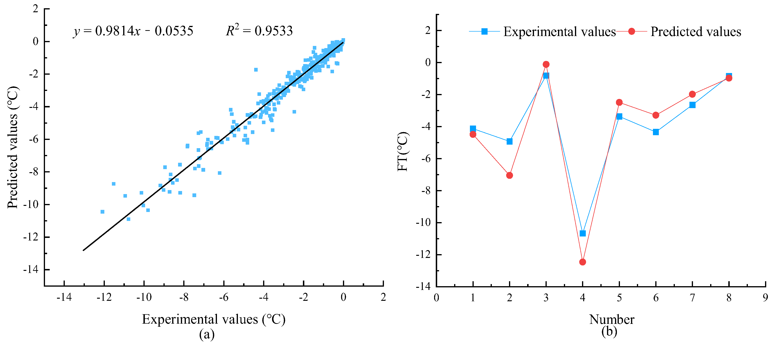
Two neural network models for predicting the freezing temperature of saline soil samples were established. The above-mentioned three statistical indicators were used to appraise the models. Figure 5 shows the measured and predicted freezing-temperature values using the BPNN method on the training and testing datasets, while Figure 6 shows the measured and predicted freezing-temperature values using the RBFNN method on the training and testing datasets. In both models, the predicted values were close to the experimental data.
Three statistical indicators of the training and test sets in the BP and RBF neural networks were calculated and are listed in Table 2. In the BPNN model, the R2, MAPD, and RMSE of the training group were 0.9533, 24.1%, and 0.533, while those of the test group were 0.9632, 12.6%, and 0.479, respectively. Additionally, in the RBFNN model, the R2, MAPD, and RMSE of the training group were 0.9796, 27.3%, and 0.352, while those of the test group were 0.9883, 26.2%, and 0.345, respectively. The above indexes show that BPNN and RBFNN methods had small prediction errors for the freezing temperature.

4. Discussion

We found that the neural network method could accurately predict the freezing temperature of multicomponent saline soil within the data range. Table 2 indicates that the R2 of BPNN and RBFNN models were both close to 1. The RMSE and MAPD values of BPNN and RBFNN models were both small. This means that the neural network method can be applied in engineering practice to prevent and restrain the engineering hazards caused by salt and frost heaving in saline soil under freezing conditions. The application of the neural network method could be roughly divided into three steps in engineering practice: First, a large number of freezing-temperature values and parameter data are collected; then, a neural network is developed after repeated testing and training, and then the model with good performance is saved; finally, soil-sample parameters are measured and inputted into the network to obtain the predicted values of freezing temperature.
Additionally, we found that the BPNN model had better performance in the data range in the comparison of the two neural network models. We observed few differences in the R2 values between BPNN and RBFNN models. This showed that these two models had similar performance in terms of prediction accuracy. Additionally, the RMSE of RBFNN was smaller than that of BFNN because RMSE is a statistic that represents an absolute error. The test data values of RBFNN were smaller than those of BPNN when their test data were randomly selected from the database. Additionally, RMSE decreased with a decrease in data. The MAPD of BPNN training data was slightly smaller than that of RBFNN, and the MAPD of the BPNN testing data was far smaller than that of RBFNN. This suggests that the BPNN method is more accurate. It can be seen from these results that the BPNN method is considered better than the RBFNN method in terms of prediction.
This phenomenon is mainly caused by their different activation functions. In BPNN, the activation function is backpropagation, while in RBFNN, the radial basis function is used as the activation function. In BPNN, the independent variable of the sigmoid function used by the hidden neuron is the inner product. Additionally, the two elements of the inner product are the input mode and the weight vector. Every hidden neuron is equally important for the result of a prediction in BPNN. Therefore, the BPNN approximates the nonlinear relation of the variable from each hidden neuron, which is called “global approximation”. In RBFNN, the independent variable of the radial basis function used by hidden neurons is the distance from the input mode to the central vector. The neuron weight decreases as the distance from the input neuron to the central neuron increases. The output of this network is closely related to the central hidden node. Therefore, one of the features of RBFNN is “local mapping”. Thus, BPNN can better predict the freezing temperature in general.
The trained BPNN model was used to compare the effects of the content of different ions on the freezing temperature. By excluding the influence of other ions, the predicted results were obtained based on each single ion variable. From the predicted results, we can compare the effect of each ion in the BPNN model. Figure 7 reveals the correlation between the contents of different ions and the freezing temperature under 10% water content. In this figure, the freezing temperature decreased linearly with the increase in ion content. If we rank the slope of the curve from highest to lowest, the order of influence of ions on the freezing temperature in the prediction model would be Cl > K+ ≈ Na+ >SO42− > CO32− > Ca2+, among which Cl had the greatest influence on the freezing temperature, and the influence of K+ and Na+ was almost slightly greater than that of SO42−, while CO32− and Ca2+ had the least effect on the freezing temperature.
Figure 8 reveals the relationship between the contents of different ions and the freezing temperature under 30% water content. The comparison between Figure 7 and Figure 8 reveals that the freezing temperature significantly decreased with the increase in water content. At 30% moisture content, the results showed that the freezing temperature almost did not change with ion content when the ion content was low, but it dramatically changed with changes in ion content when the ion content was high. The order of the ions’ influences on the freezing temperature also changed. The order after change was K+ > Cl > SO42− > Na+ >CO32− > Ca2+. The influence of K+ with the increase in water content exceeded that of Cl, while SO42− was also more influential than Na+.
Although there are many factors that can affect the freezing temperature of multicomponent saline soil, we could only establish the prediction models based on ion content, water content, and soluble salt content due to data limitations. In this paper, we used two of the most basic and widely used models to make predictions, and there are many models that might perform better. In future studies, researchers may use more methods and parameters to predict the freezing temperature of multicomponent saline soils.

5. Conclusions

In this paper, BPNN and RBFNN models for predicting the freezing temperature of saline soil were established. The freezing temperature of the corresponding sample could be obtained by inputting the required parameters (ion content, water content, and soluble salt content) into the model. BPNN and RBFNN models were utilized to predict the freezing temperature of the samples with different values for the above parameters. From the aforementioned two prediction models, we drew the following conclusions:
Firstly, overall, the measured values were very close to the predicted values from the output of BPNN and RBFNN methods. The R2, RMSE and MAPD values of BPNN and RBFNN indicate that these two kinds of networks are appropriate for predicting freezing temperatures.
Furthermore, the BPNN model was more precise than the BRFNN model in the data range used in this article. The statistical comparison between BPNN and RBFNN shows that BPNN is a more appropriate method to establish a dependable freezing temperature prediction model.
Finally, using the trained BPNN model for data simulation, the order of influence on the freezing temperature of ions was Cl > K+ ≈ Na+ > SO42− > CO32− > Ca2+ under the water content of 10%, while the order of influence on the freezing temperature of ions was K+ > Cl > SO42− > Na+ >CO32− > Ca2+ under the water content of 30%.

Author Contributions

Conceptualization, J.D. and Z.X.; methodology, J.D.; software, J.D.; validation, J.D., Z.X. and L.Z.; formal analysis, J.D.; investigation, K.L.; resources, Z.X.; data curation, J.D.; writing—original draft preparation, J.D.; writing—review and editing, J.D. and Z.X.; visualization, J.D.; supervision, Z.X.; project administration, Z.X.; funding acquisition, Z.X. All authors have read and agreed to the published version of the manuscript.

Funding

This research was funded by National Natural Science Foundation of China grant number [42271137].

Institutional Review Board Statement

Not applicable.

Informed Consent Statement

Not applicable.

Data Availability Statement

No new data were created or analyzed in this study. Data sharing is not applicable to this article.

Acknowledgments

This research was supported by the National Natural Science Foundation of China (42271137).

Conflicts of Interest

The authors declare no conflict of interest.

References

  1. Xu, X.Z.; Wang, J.C.; Zhang, L.X.; Deng, Y.S. Mechanisms of Frost Heave and Soil Expansion of Soils; Science Press: Beijing, China, 1995. [Google Scholar]
  2. Xu, X.Z.; Wang, J.C.; Zhang, L.X. Frozen Soil Physics; Science Press: Beijing, China, 2010. [Google Scholar]
  3. Qiu, K.; Ding, L.; Yu, W.; Chen, K.; Huang, S.; Gao, K. Experimental Investigation of Shear Strength of Carbonate Saline Soil under Freeze-Thaw Cycles. Atmosphere 2022, 13, 2063. [Google Scholar] [CrossRef]
  4. Chun-lei, W.A.; Qiang, X.I.; Chong-xi, J.I. Analysis of thermal characteristics and mechanical properties of salty soil in frozen area of Qinghai-Tibet Railway. Rock Soil Mech. 2009, 3, 836–839. [Google Scholar]
  5. Tan, D.S.; Sun, Y.M.; Hu, L.X.; Jiang, F.Q.; Zhang, F.L. Salt expansion properties and mechanism of saline soil in Xinjiang section of Lanzhou–Xinjiang railway and preventive measures. J. China Railw. Soc. 2011, 33, 83–88. [Google Scholar]
  6. Cui, G.X. Determination of freezing temperature and thickness of frozen wall in wet soil with thick topsoil. J. China Univ. Min. Technol. 1997, 3, 3–6. [Google Scholar]
  7. Liu, J.K. Influence of nonuniform distribution of fine soil on mechanical properties of coarse-grained soil. Chin. J. Geotech. Eng. 2017, 39, 562–572. [Google Scholar]
  8. Hu, T.F.; Liu, J.; Fang, J. Experimental study on the effect of cyclic freezing-thawing on mechanical properties of silty clay under different cooling temperatures. Chin. J. Rock Mech. Eng. 2017, 33, 1496–1502. [Google Scholar]
  9. Wang, Z.J. Influence of freezing and thawing on collapsibility of loess. Chin. J. Undergr. Space Eng. 2016, 12, 1710–1716. [Google Scholar]
  10. Yingjun, S.O.; Lei, X.U.; Yang, L.U. Experimental studies on freeze-thaw cycles of expansive soil based on orthogonal design. J. Water Resour. Hydropower Eng. 2017, 2, 51–58. [Google Scholar]
  11. Xiao, Z.A.; Lai, Y.M.; You, Z.M. Water and salt migration and deformation mechanism of sodium chloride soil during unidirectional freezing process. Chin. J. Geotech. Eng. 2017, 39, 1992–2001. [Google Scholar]
  12. Li, G.; Li, N.; Liu, N.; Zhu, C. Practical algorithm of THM coupling process with ice-water phase change based on FLAC3D. Chin. J. Rock Mech. Eng. 2017, 36 (Suppl. 2), 3841–3851. [Google Scholar]
  13. Banin, A.; Anderson, D.M. Effects of salt concentration changes during freezing on the unfrozen water content of porous materials. Water Resour. Res. 1974, 10, 124–128. [Google Scholar] [CrossRef]
  14. Kozlowski, T. A comprehensive method of determining the soil unfrozen water curves: 2. stages of the phase change process in frozen soil–water system. Cold Reg. Sci. Technol. 2003, 36, 81–92. [Google Scholar] [CrossRef]
  15. Bing, H.; Ma, W. Laboratory investigation of the freezing point of saline soil. Cold Reg. Sci. Technol. 2011, 67, 79–88. [Google Scholar] [CrossRef]
  16. Low, P.F.; Anderson, D.M.; Hoekstra, P. Some thermodynamic relationships for soils at or below the freezing point: 1. Freezing point depression and heat capacity. Water Resour. Res. 1968, 4, 379–394. [Google Scholar] [CrossRef] [Green Version]
  17. Azmatch, T.F.; Sego, D.C.; Arenson, L.U.; Biggar, K.W. Using soil freezing characteristic curve to estimate the hydraulic conductivity function of partially frozen soils. Cold Reg. Sci. Technol. 2012, 83, 103–109. [Google Scholar] [CrossRef]
  18. Wan, X.S.; Lai, Y.M.; Wang, C. Experimental Study on freezing temperatures of Saline Silty Soils. Permafr. Periglac. Process. 2015, 26, 175–187. [Google Scholar] [CrossRef]
  19. Wan, X.S.; Lai, Y.M. Experimental study on freezing temperature and salt crystal precipitation of sodium sulphate soulotion and sodium sulphate saline soil. Chin. J. Geotech. Eng. 2013, 35, 2090–2096. [Google Scholar]
  20. Xiao, Z.A.; Lai, Y.M.; Zhang, M.Y. Study on freezing temperature of saline soil. Acta Geotech. 2018, 13, 195–205. [Google Scholar] [CrossRef]
  21. Wang, Q.; Qi, J.; Wang, S.; Xu, J.; Yang, Y. Effect of freeze-thaw on freezing point of a saline loess. Cold Reg. Sci. Technol. 2020, 170, 102922. [Google Scholar] [CrossRef]
  22. Adeli, H. Neural networks in civil engineering: 1989–2000. Comput. -Aided Civ. Infrastruct. Eng. 2001, 16, 126–142. [Google Scholar] [CrossRef]
  23. Wu, X.; Ghaboussi, J.; Garrett, J.H., Jr. Use of neural networks in detection of structural damage. Comput. Struct. 1992, 42, 649–659. [Google Scholar] [CrossRef]
  24. Mohamad, E.T.; Jahed Armaghani, D.; Momeni, E.; Alavi Nezhad Khalil Abad, S.V. Prediction of the unconfined compressive strength of soft rocks: A PSO-based ANN approach. Bull. Eng. Geol. Environ. 2015, 74, 745–757. [Google Scholar] [CrossRef]
  25. Hajihassani, M.; Armaghani, D.J.; Marto, A.; Mohamad, E.T. Ground vibration prediction in quarry blasting through an artificial neural network optimized by imperialist competitive algorithm. Bull. Eng. Geol. Environ. 2015, 74, 873–886. [Google Scholar] [CrossRef]
  26. Wang, B.; Man, T.; Jin, H. Prediction of expansion behavior of self-stressing concrete by artificial neural networks and fuzzy inference systems. Constr. Build. Mater. 2015, 84, 184–191. [Google Scholar] [CrossRef]
  27. Sun, J.Z. Study on Thaw Settlement Characteristics of Chloride Saline Soil Based on BP Neural Network. J. Lanzhou Jiaotong Univ. 2020, 39, 26–31. [Google Scholar]
  28. Moody, J.; Darken, C.J. Fast learning in networks of locally-tuned processing units. Neural Comput. 1989, 1, 281–294. [Google Scholar] [CrossRef]
  29. Sun, D.Y. Characteristics and Prediction of Frost Heave of Saline Soil in Western Jilin Province. Int. J. Heat Technol. 2016, 34, 709–714. [Google Scholar] [CrossRef]
  30. Fagerlund, G. Determination of pore-size distribution from freezing point depression. Mater. Struct. 1973, 6, 215–225. [Google Scholar] [CrossRef]
  31. Sun, Z.; Scherer, G.W. Pore size and shape in mortar by thermoporometry. Cem. Concr. Res. 2010, 40, 740–751. [Google Scholar] [CrossRef]
  32. Zhang, X.; Wang, Q.; Huo, Z.; Yu, T.; Wang, G.; Liu, T.; Wang, W. Prediction of Frost-Heaving Behavior of Saline Soil in Western Jilin Province, China, by Neural Network Methods. Math. Probl. Eng. 2017, 2017, 7689415. [Google Scholar] [CrossRef] [Green Version]
  33. Seshagiri, S.; Khalil, H.K. Output feedback control of nonlinear systems using RBF neural networks. IEEE Trans. Neural Netw. 2000, 11, 69–79. [Google Scholar] [CrossRef] [PubMed] [Green Version]
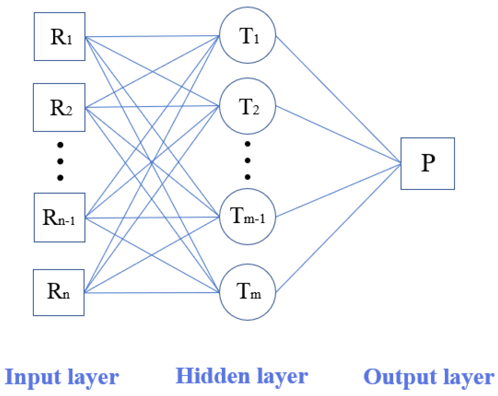
Figure 1. The architecture of neural network predictor model.
Atmosphere 14 00422 g001
Figure 2. Statistical indicators with different numbers of hidden-layer units in BPNN: (a) R2; (b) RMSE; (c) MAPD. The red part represents the hidden layer unit eventually adopted, and the blue part represents other units within the range.
Atmosphere 14 00422 g002
Figure 3. Statistical indicators with the whole number of hidden-layer units in RBFNN between 0 and 100: (a) R2; (b) RMSE; (c) MAPD. The red part represents the best performing hidden layer unit, and the blue part represents other units within the range.
Atmosphere 14 00422 g003
Figure 4. Statistical indicators with the number of hidden-layer units in RBFNN between 26 and 34: (a) R2; (b) RMSE; (c) MAPD. The red part represents the hidden layer unit eventually adopted, and the blue part represents other units within the range.
Atmosphere 14 00422 g004
Figure 5. Comparison of predicted and experimental values for the BPNN model: (a) training values; (b) testing values.
Atmosphere 14 00422 g005
Figure 6. Comparison of predicted and experimental values for the RBFNN model: (a) training values; (b) testing values.
Atmosphere 14 00422 g006
Figure 7. The relationship between freezing temperature and the content of each ion under 10% water content.
Atmosphere 14 00422 g007
Figure 8. The relationship between freezing temperature and the content of each ion under 30% water content.
Atmosphere 14 00422 g008
Table 1. The distribution of 367 data values of the freezing temperature of the soil.
Group1234567
Number112795246261111
Group891011121314
Number11835111
Table 2. Statistical indicators of training and testing data in BPNN and RBFNN.
NetDataR2RMSEMAPD
BPNNTraining data0.95330.53324.1%
Testing data0.96320.47912.6%
RBFNNTraining data0.97960.35227.3%
Testing data0.98830.34526.2%
Disclaimer/Publisher’s Note: The statements, opinions and data contained in all publications are solely those of the individual author(s) and contributor(s) and not of MDPI and/or the editor(s). MDPI and/or the editor(s) disclaim responsibility for any injury to people or property resulting from any ideas, methods, instructions or products referred to in the content.