
Development of a New Analytical Method for the Characterization and Quantification of the Organic and Inorganic Carbonaceous Fractions in Snow Samples Using TOC and TOT Analysis
 ,
,  ,
,  ,
,  , , ,
, , ,  and
and 
Abstract
:1. Introduction
- BC: Black Carbon, carbonaceous material that displays the following five properties [18]. Continuous, wavelength-independent absorption of visible light; at 550 nm, BC shows a Mass Absorption Coefficient (MAC) of 5 m2 g−1 or more. It exhibits refractory properties at vaporization temperatures above 4000 K; gasification is possible only by oxidation above 340 °C. It has a graphitic structure and a fractal-like chain-aggregate morphology. It is insoluble in water and in most common organic solvents.
2. Materials and Methods
2.1. Analytical Methods: State of the Art (S.A.)
2.1.1. S.A.—Sampling
2.1.2. S.A.—Sample Pre-Treatment
2.1.3. S.A.—Sample Melting
2.1.4. S.A.—Filtration
2.1.5. S.A.—Analysis
2.2. The Analyzed Snow Samples and the Applied Method
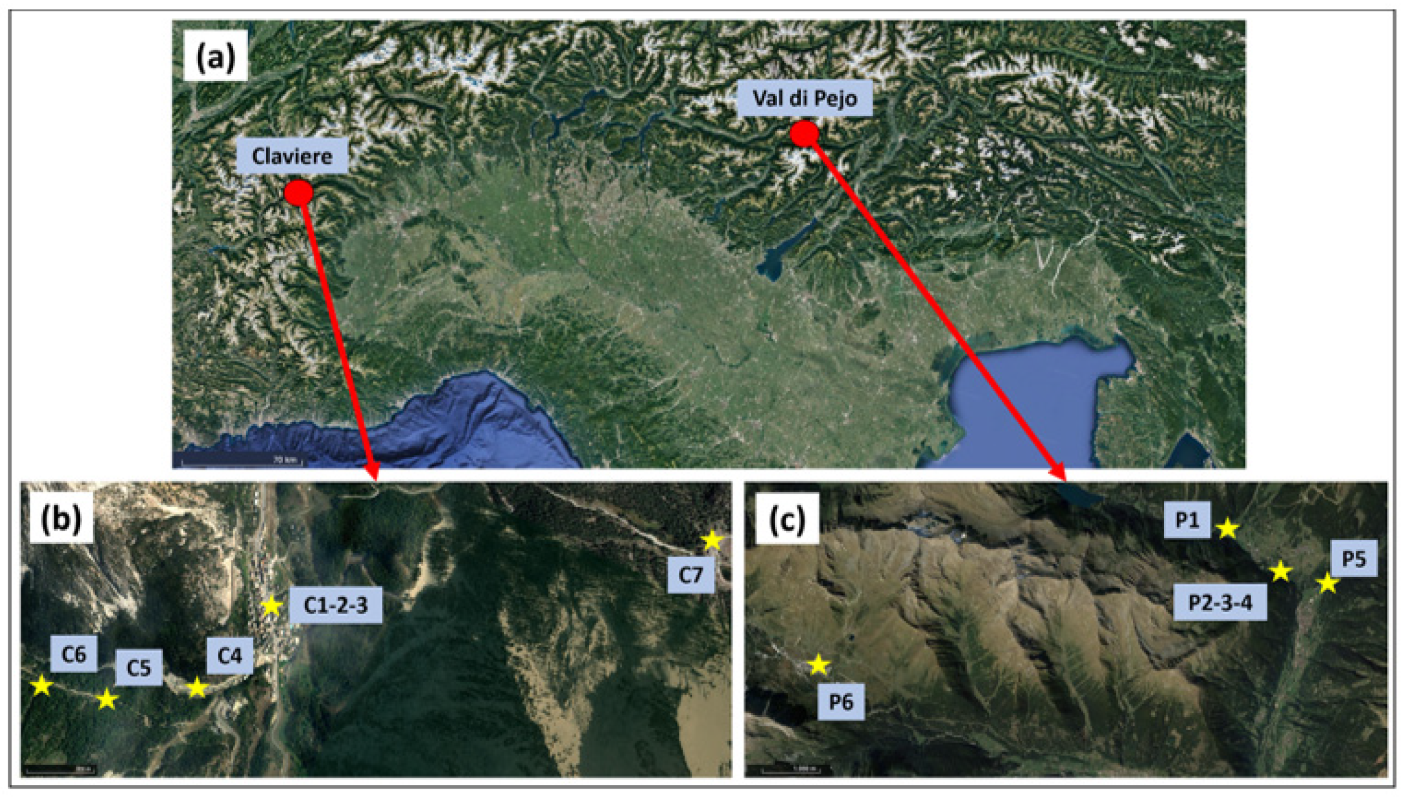
2.2.1. Sampling Procedure and Description of the Samples
2.2.2. Analytical Techniques
- TC analyzed by burning the entire injected aliquot. All carbonaceous species were converted into carbon dioxide;
- IC, which evolves into carbon dioxide after acidification (pH < 3) and sample purging;
- NPOC, which corresponds to TC determined after purging for IC quantification;
- POC, Purgeable Organic Carbon, which evolves together with IC and is not revealed directly.
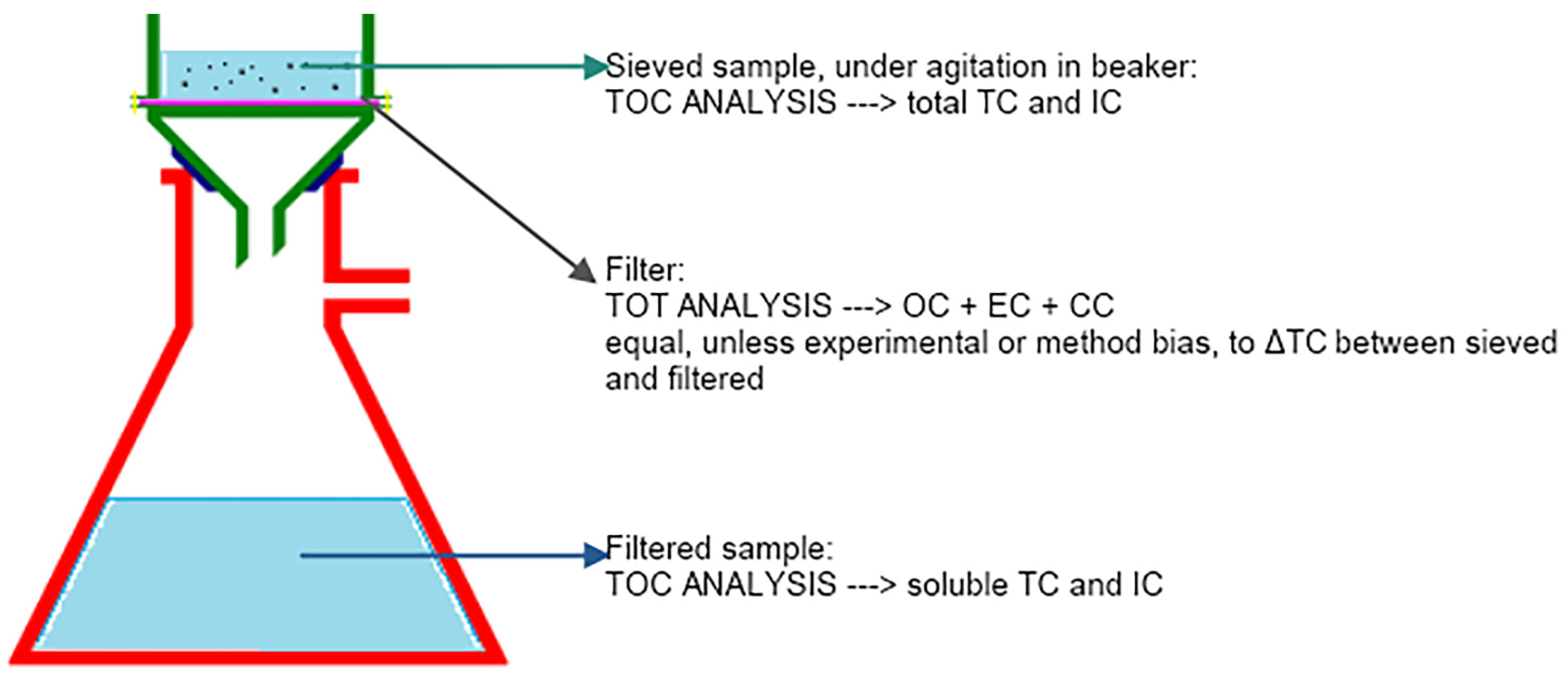
2.2.3. Work Scheme
- directly by TOT analysis on the filter;
- using TOC analysis and calculating the difference between the concentrations found in the sieved suspension and the filtered solution.
2.2.4. Sample Melting
2.2.5. Sieving
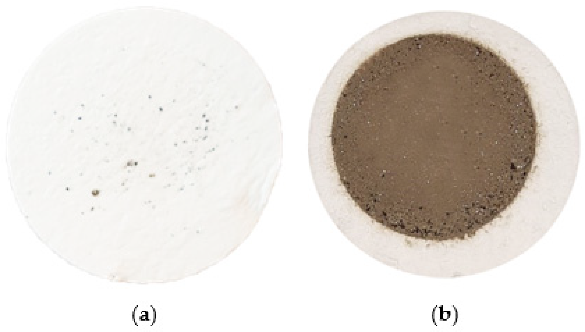
2.2.6. Filtration
2.2.7. Analysis
/Vol (filtered)
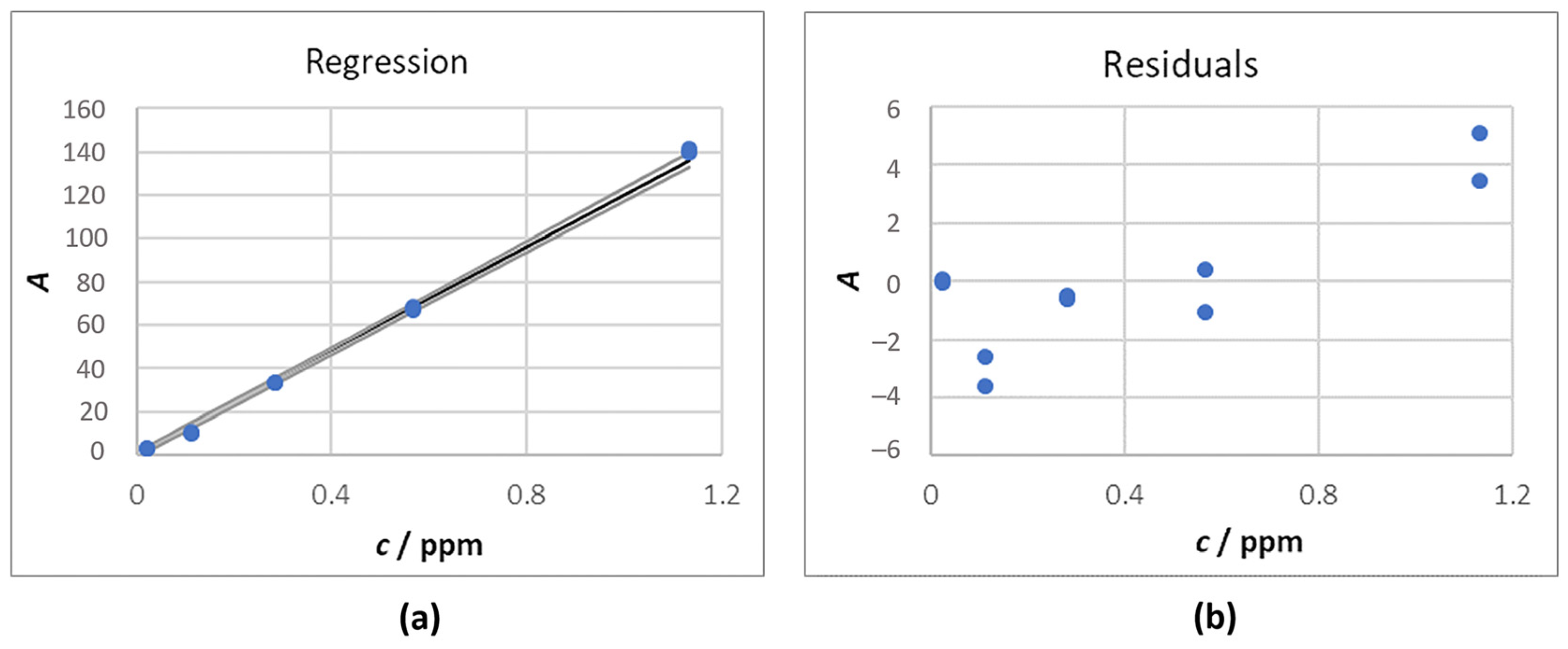
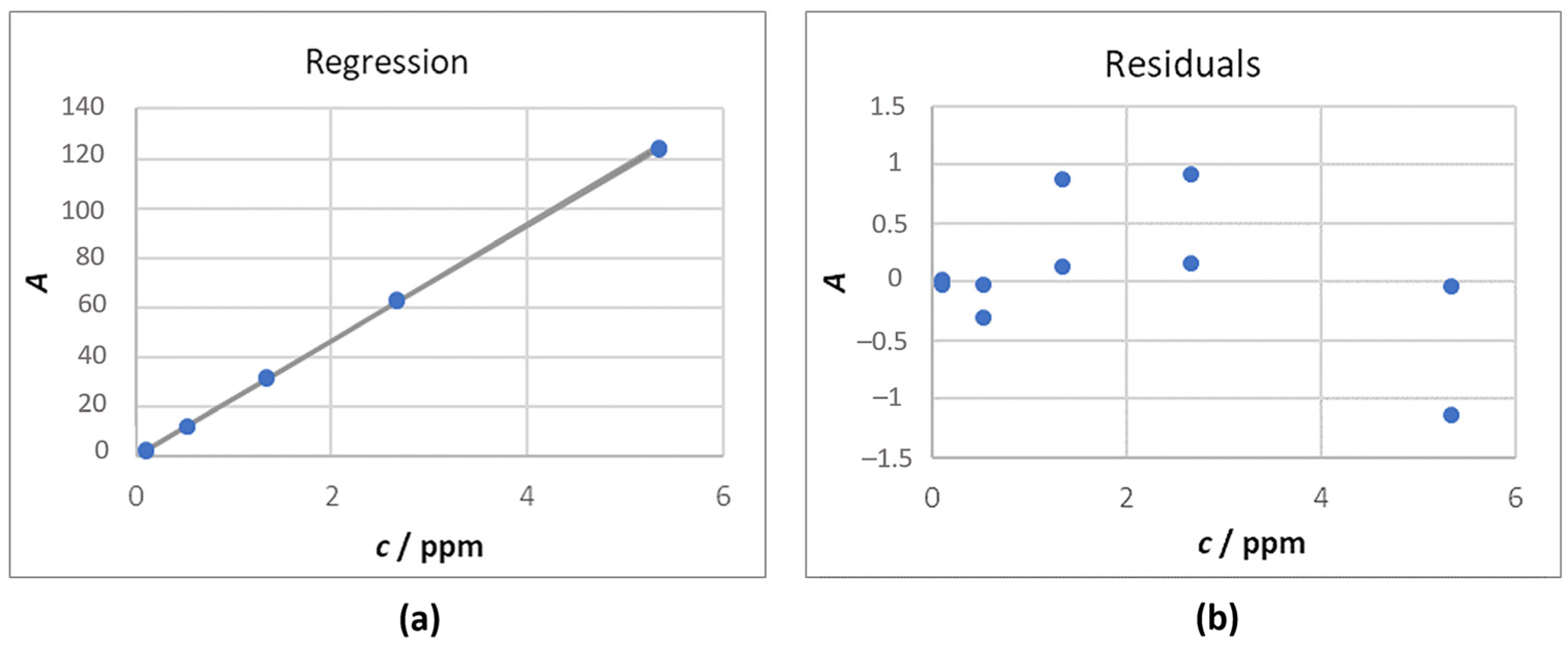
2.2.8. Quality Control
3. Results
3.1. TOC Analysis Results
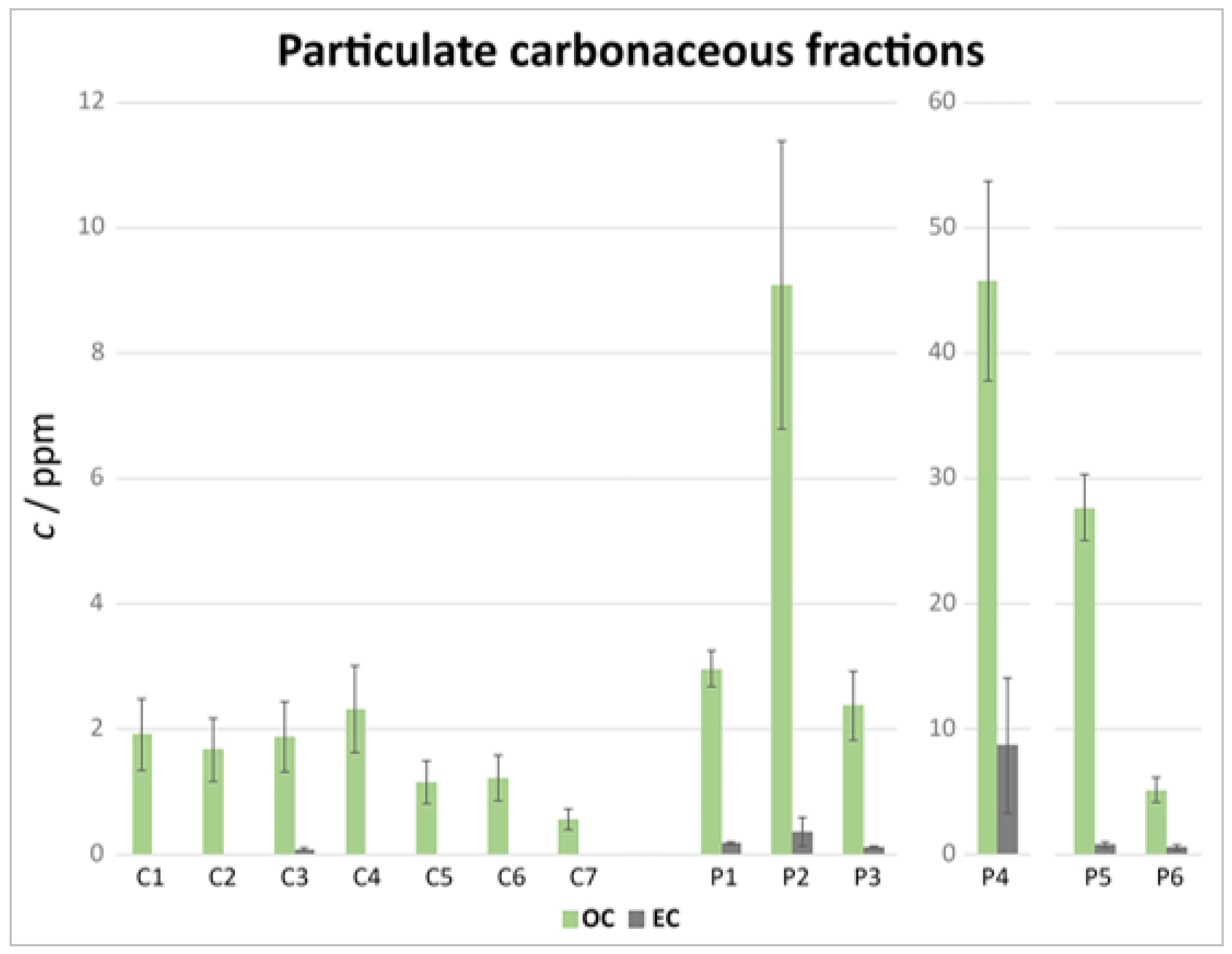
3.2. TOT Analysis Results
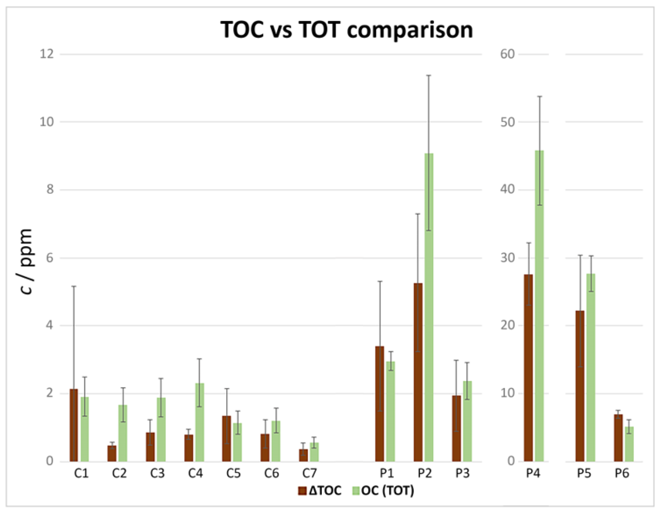
3.3. TOC and TOT Comparison
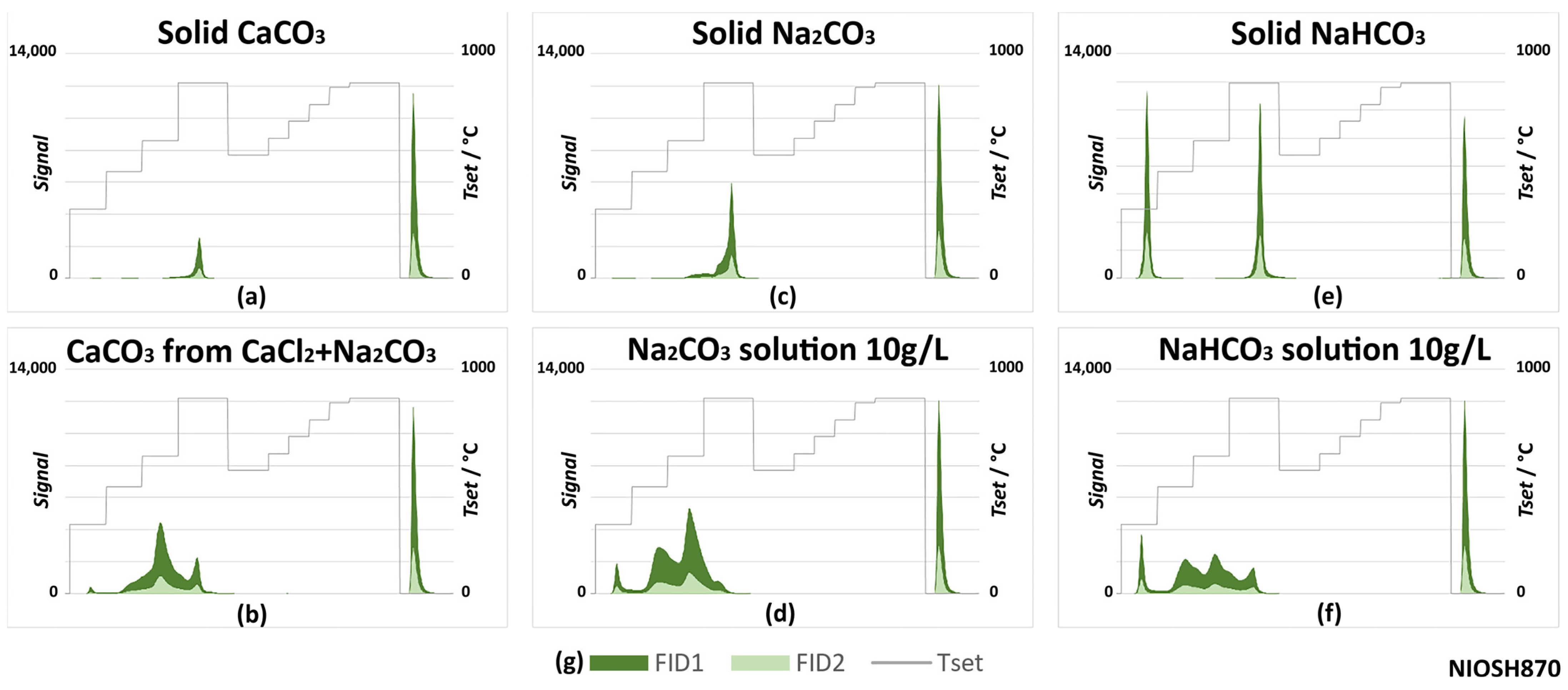
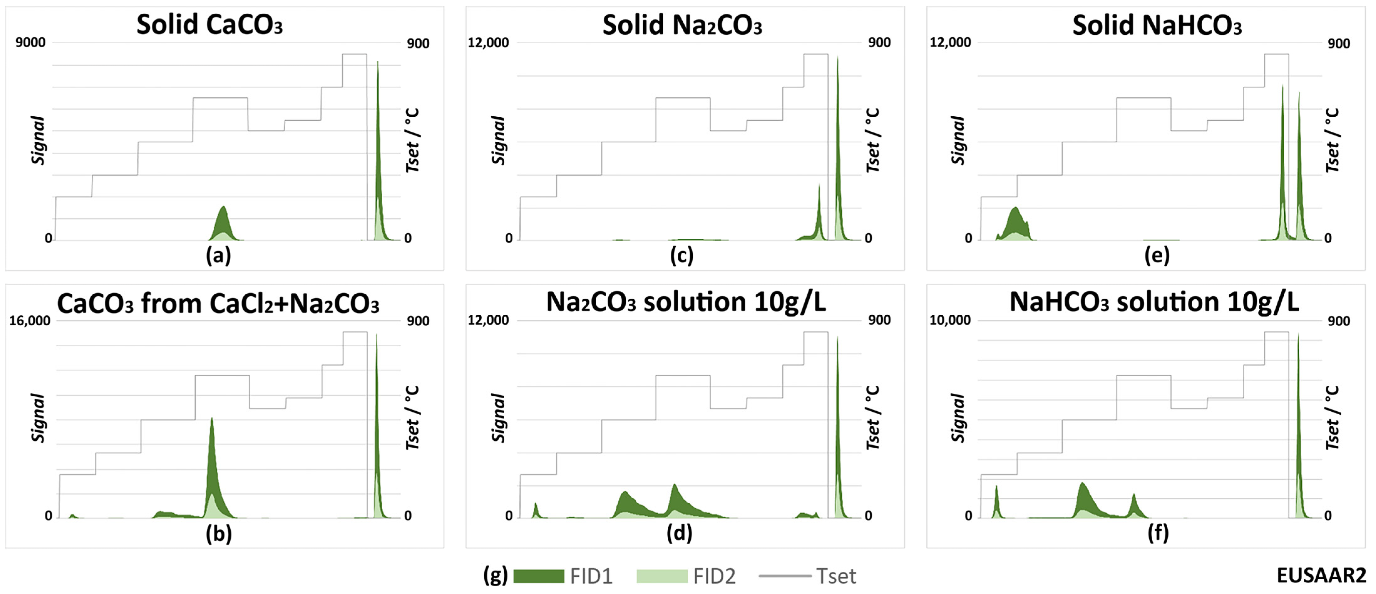
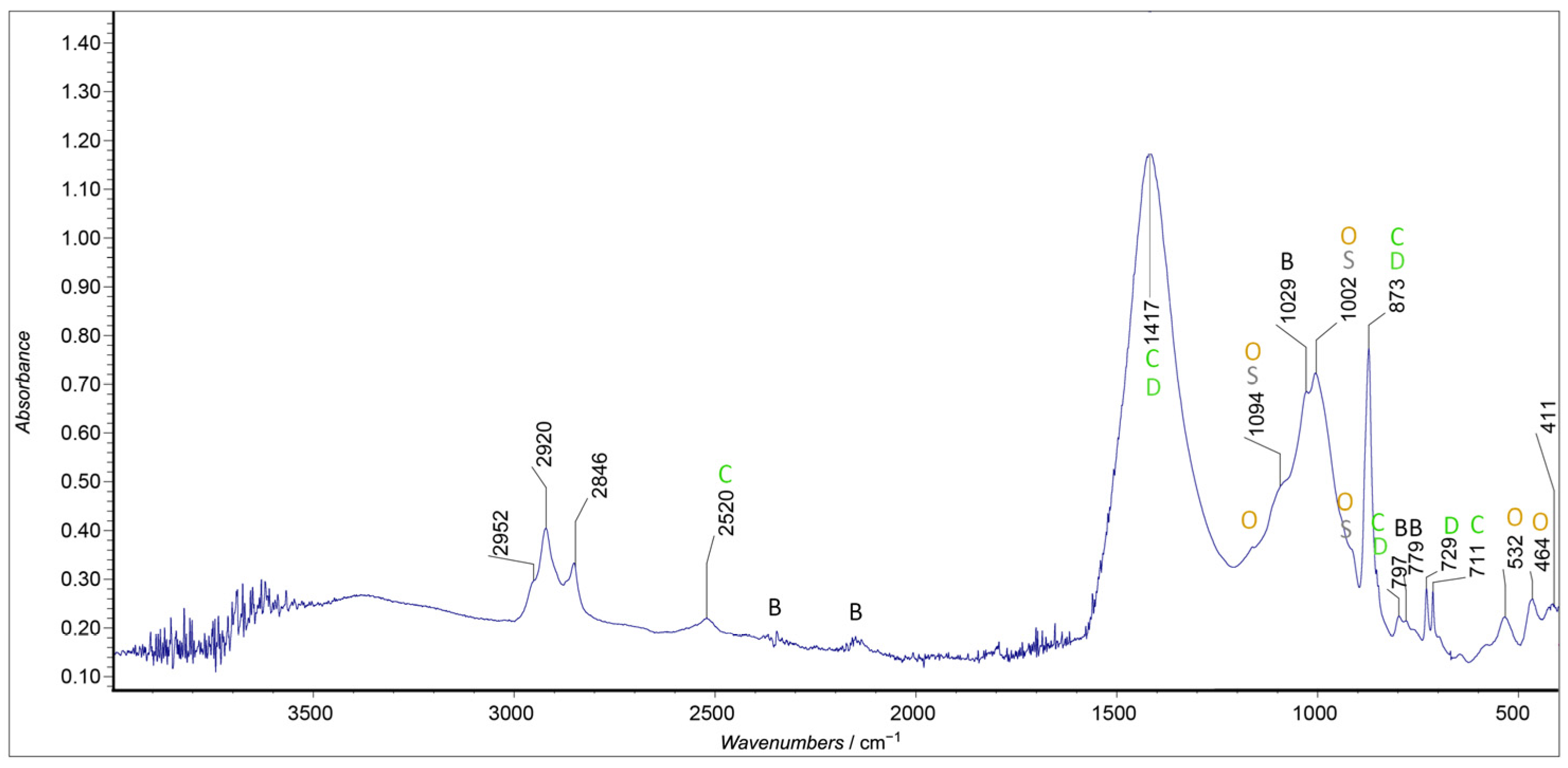
3.4. ATR-FTIR Results
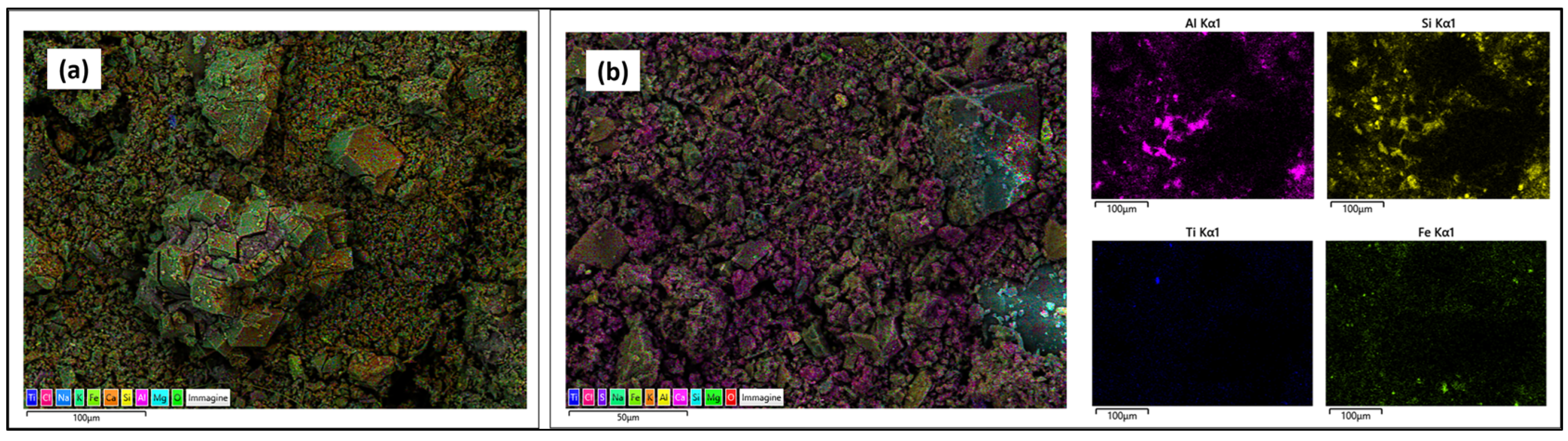
3.5. SEM-EDX Analysis Results
4. Discussion
4.1. Blank Analysis
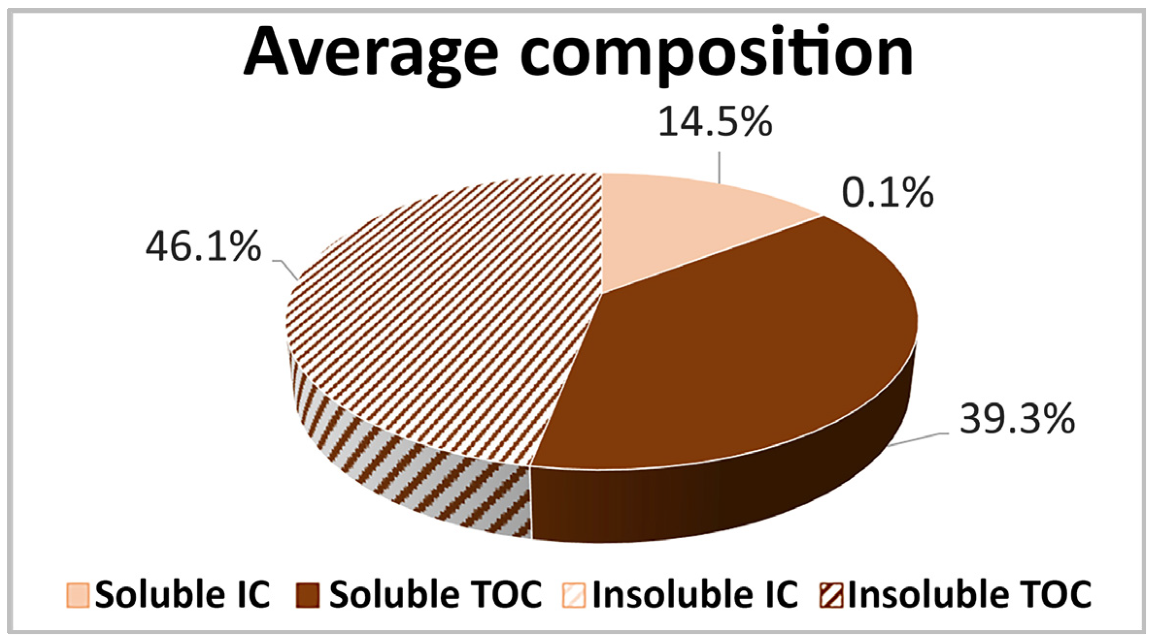
4.2. Comments on the Snow Sample Composition
4.3. Inorganic Carbon
4.4. Larger Particles
5. Conclusions
Supplementary Materials
Author Contributions
Funding
Institutional Review Board Statement
Informed Consent Statement
Data Availability Statement
Conflicts of Interest
References
- Wang, X.; Wei, H.; Liu, J.; Xu, B.; Wang, M.; Ji, M.; Jin, H. Quantifying the Light Absorption and Source Attribution of Insoluble Light-Absorbing Particles on Tibetan Plateau Glaciers between 2013 and 2015. Cryosphere 2019, 13, 309–324. [Google Scholar] [CrossRef]
- Skiles, S.M.K.; Flanner, M.; Cook, J.M.; Dumont, M.; Painter, T.H. Radiative Forcing by Light-Absorbing Particles in Snow. Nat. Clim. Change 2018, 8, 964–971. [Google Scholar] [CrossRef]
- IPCC Special Report: The Ocean and Cryosphere in a Changing Climate. 2019. Available online: https://www.ipcc.ch/report/srocc/ (accessed on 10 December 2022).
- di Mauro, B. A Darker Cryosphere in a Warming World. Nat. Clim. Chang. 2020, 10, 979–980. [Google Scholar] [CrossRef]
- Hamilton, T.L.; Havig, J.R. Inorganic Carbon Addition Stimulates Snow Algae Primary Productivity. ISME J. 2020, 14, 857–860. [Google Scholar] [CrossRef]
- John Maurer Retrieval of Surface Albedo from Space. Available online: http://www2.hawaii.edu/~jmaurer/albedo/ (accessed on 20 December 2022).
- Kuchiki, K.; Aoki, T.; Niwano, M.; Matoba, S.; Kodama, Y.; Adachi, K. Elemental Carbon, Organic Carbon, and Dust Concentrations in Snow Measured with Thermal Optical and Gravimetric Methods: Variations during the 2007-2013 Winters at Sapporo, Japan. J. Geophys. Res. Atmos. 2015, 120, 868–882. [Google Scholar] [CrossRef]
- Ielpo, P.; Mangia, C.; de Gennaro, G.; di Gilio, A.; Palmisani, J.; Dinoi, A.; Bergomi, A.; Comite, V.; Fermo, P. Air Quality Assessment of a School in an Industrialized Area of Southern Italy. Appl. Sci. 2021, 11, 8870. [Google Scholar] [CrossRef]
- Bergomi, A.; Morreale, C.; Fermo, P.; Migliavacca, G. Determination of Pollutant Emissions from Wood-Fired Pizza Ovens. Chem. Eng. Trans. 2022, 92, 499–504. [Google Scholar] [CrossRef]
- di Mauro, B.; Fava, F.; Ferrero, L.; Garzonio, R.; Baccolo, G.; Delmonte, B.; Colombo, R. Mineral Dust Impact on Snow Radiative Properties in the European Alps Combining Ground, UAV, and Satellite Observations. J. Geophys. Res. Atmos. 2015, 120, 6080–6097. [Google Scholar] [CrossRef]
- Kinase, T.; Kita, K.; Tsukagawa-Ogawa, Y.; Goto-Azuma, K.; Kawashima, H. Influence of the Melting Temperature on the Measurement of the Mass Concentration and Size Distribution of Black Carbon in Snow. Atmos. Meas. Tech. 2016, 9, 1939–1945. [Google Scholar] [CrossRef]
- Keil, A.; Haywood, J.M. Solar Radiative Forcing by Biomass Burning Aerosol Particles during SAFARI 2000: A Case Study Based on Measured Aerosol and Cloud Properties. J. Geophys. Res. Atmos. 2003, 108, SAF3-1. [Google Scholar] [CrossRef]
- Doherty, S.J.; Grenfell, T.C.; Forsström, S.; Hegg, D.L.; Brandt, R.E.; Warren, S.G. Observed Vertical Redistribution of Black Carbon and Other Insoluble Light-Absorbing Particles in Melting Snow. J. Geophys. Res. Atmos. 2013, 118, 5553–5569. [Google Scholar] [CrossRef]
- Aamaas, B.; Bøggild, C.E.; Stordal, F.; Berntsen, T.; Holmén, K.; Ström, J. Elemental Carbon Deposition to Svalbard Snow from Norwegian Settlements and Long-Range Transport. Tellus B Chem. Phys. Meteorol. 2011, 63, 340. [Google Scholar] [CrossRef]
- Hagler, G.S.W.; Bergin, M.H.; Smith, E.A.; Dibb, J.E.; Anderson, C.; Steig, E.J. Particulate and Water-Soluble Carbon Measured in Recent Snow at Summit, Greenland. Geophys. Res. Lett. 2007, 34, L16505. [Google Scholar] [CrossRef]
- Cuccia, E.; Gianelle, V.; Dal Santo, U.; Colombi, C. Campagna Di Misura Della Qualità Dell’Aria—Relazione Finale—Comune Di Rezzato; ARPA Lombardia: Milan, Italy, 2017. [Google Scholar]
- Lack, D.A.; Moosmüller, H.; McMeeking, G.R.; Chakrabarty, R.K.; Baumgardner, D. Characterizing Elemental, Equivalent Black, and Refractory Black Carbon Aerosol Particles: A Review of Techniques, Their Limitations and Uncertainties. Anal. Bioanal. Chem. 2013, 406, 99–122. [Google Scholar] [CrossRef]
- Petzold, A.; Ogren, J.A.; Fiebig, M.; Laj, P.; Li, S.M.; Baltensperger, U.; Holzer-Popp, T.; Kinne, S.; Pappalardo, G.; Sugimoto, N.; et al. Recommendations for Reporting Black Carbon Measurements. Atmos. Meas. Tech. 2013, 13, 8365–8379. [Google Scholar] [CrossRef]
- Beres, N.D.; Sengupta, D.; Samburova, V.; Khlystov, A.Y.; Moosmüller, H. Deposition of Brown Carbon onto Snow: Changes in Snow Optical and Radiative Properties. Atmos. Chem. Phys. 2020, 20, 6095–6114. [Google Scholar] [CrossRef]
- Lin, P.; Liu, J.; Shilling, J.E.; Kathmann, S.M.; Laskin, J.; Laskin, A. Molecular Characterization of Brown Carbon (BrC) Chromophores in Secondary Organic Aerosol Generated from Photo-Oxidation of Toluene. Phys. Chem. Chem. Phys. 2015, 17, 23312–23325. [Google Scholar] [CrossRef]
- Ming, J.; Xiao, C.; Cachier, H.; Qin, D.; Qin, X.; Li, Z.; Pu, J. Black Carbon (BC) in the Snow of Glaciers in West China and Its Potential Effects on Albedos. Atmos. Res. 2009, 92, 114–123. [Google Scholar] [CrossRef]
- Legrand, M.; Preunkert, S.; Jourdain, B.; Guilhermet, J.; Faïn, X.; Alekhina, I.; Petit, J.R. Water-Soluble Organic Carbon in Snow and Ice Deposited at Alpine, Greenland, and Antarctic Sites: A Critical Review of Available Data and Their Atmospheric Relevance. Clim. Past 2013, 9, 2195–2211. [Google Scholar] [CrossRef]
- Wang, X.; Doherty, S.J.; Huang, J. Black Carbon and Other Light-Absorbing Impurities in Snow across Northern China. J. Geophys. Res. Atmos. 2013, 118, 1471–1492. [Google Scholar] [CrossRef]
- Zhang, Y.; Kang, S.; Gao, T.; Schmale, J.; Liu, Y.; Zhang, W.; Guo, J.; Du, W.; Hu, Z.; Cui, X.; et al. Dissolved Organic Carbon in Snow Cover of the Chinese Altai Mountains, Central Asia: Concentrations, Sources and Light-Absorption Properties. Sci. Total Environ. 2019, 647, 1385–1397. [Google Scholar] [CrossRef]
- Kawamura, K.; Matsumoto, K.; Tachibana, E.; Aoki, K. Low Molecular Weight (C 1-C 10) Monocarboxylic Acids, Dissolved Organic Carbon and Major Inorganic Ions in Alpine Snow Pit Sequence from a High Mountain Site, Central Japan. Atmos. Environ. 2012, 62, 272–280. [Google Scholar] [CrossRef]
- Doherty, S.J.; Dang, C.; Hegg, D.A.; Zhang, R.; Warren, S.G. Black Carbon and Other Light-Absorbing Particles in Snow of Central North America. J. Geophys. Res. Atmos. 2014, 119, 12–807. [Google Scholar] [CrossRef]
- Lim, S.; Faïn, X.; Zanatta, M.; Cozic, J.; Jaffrezo, J.L.; Ginot, P.; Laj, P. Refractory Black Carbon Mass Concentrations in Snow and Ice: Method Evaluation and Inter-Comparison with Elemental Carbon Measurement. Atmos. Meas. Tech. 2014, 7, 3307–3324. [Google Scholar] [CrossRef]
- Schwarz, J.P.; Gao, R.S.; Perring, A.E.; Spackman, J.R.; Fahey, D.W. Black Carbon Aerosol Size in Snow. Sci. Rep. 2013, 3, 1356. [Google Scholar] [CrossRef]
- Meinander, O.; Heikkinen, E.; Aurela, M.; Hyvärinen, A. Sampling, Filtering, and Analysis Protocols to Detect Black Carbon, Organic Carbon, and Total Carbon in Seasonal Surface Snow in an Urban Background and Arctic Finland (>60° N). Atmosphere 2020, 11, 923. [Google Scholar] [CrossRef]
- Svensson, J.; Ström, J.; Kivekäs, N.; Dkhar, N.B.; Tayal, S.; Sharma, V.P.; Jutila, A.; Backman, J.; Virkkula, A.; Ruppel, M.; et al. Light-Absorption of Dust and Elemental Carbon in Snow in the Indian Himalayas and the Finnish Arctic. Atmos. Meas. Tech. 2018, 11, 1403–1416. [Google Scholar] [CrossRef]
- Cavalli, F.; Viana, M.; Yttri, K.E.; Genberg, J.; Putaud, J.P. Toward a Standardised Thermal-Optical Protocol for Measuring Atmospheric Organic and Elemental Carbon: The EUSAAR Protocol. Atmos. Meas. Tech. 2010, 3, 79–89. [Google Scholar] [CrossRef]
- He, C.; Takano, Y.; Liou, K.N.; Yang, P.; Li, Q.; Chen, F. Impact of Snow Grain Shape and Black Carbon-Snow Internal Mixing on Snow Optical Properties: Parameterizations for Climate Models. J. Clim. 2017, 30, 10019–10036. [Google Scholar] [CrossRef]
- Bautista, A.T.; Pabroa, P.C.B.; Santos, F.L.; Quirit, L.L.; Asis, J.L.B.; Dy, M.A.K.; Martinez, J.P.G. Intercomparison between NIOSH, IMPROVE_A, and EUSAAR_2 Protocols: Finding an Optimal Thermal-Optical Protocol for Philippines OC/EC Samples. Atmos. Pollut. Res. 2015, 6, 334–342. [Google Scholar] [CrossRef]
- Giannoni, M.; Calzolai, G.; Chiari, M.; Cincinelli, A.; Lucarelli, F.; Martellini, T.; Nava, S. A Comparison between Thermal-Optical Transmittance Elemental Carbon Measured by Different Protocols in PM2.5 Samples. Sci. Total Environ. 2016, 571, 195–205. [Google Scholar] [CrossRef]
- Ashley, K.; O’Connor, P.F. NIOSH Manual of Analytical Methods (NMAM), 5th ed.; Cdc, 2017. Available online: https://www.cdc.gov/niosh/nmam/pdfs/nmam_5thed_ebook.pdf (accessed on 17 May 2022).
- Kuchiki, K.; Aoki, T.; Niwano, M. Possible Causes of Error in Measurement of Mass Concentration of Snow Impurities –Effects of a Filter and Carbonate Carbon. In Proceedings of the Summaries of JSSI and JSSE Joint Conference on Snow and Ice Research; 2010; Volume 2010. [Google Scholar] [CrossRef]
- Sala, M.; Delmonte, B.; Frezzotti, M.; Proposito, M.; Scarchilli, C.; Maggi, V.; Artioli, G.; Dapiaggi, M.; Marino, F.; Ricci, P.C.; et al. Evidence of Calcium Carbonates in Coastal (Talos Dome and Ross Sea Area) East Antarctica Snow and Firn: Environmental and Climatic Implications. Earth Planet. Sci. Lett. 2008, 271, 43–52. [Google Scholar] [CrossRef]
- Clow, D.W.; Ingersoll, G.P. Particulate Carbonate Matter in Snow from Selected Sites in the South-Central Rocky Mountains. Atmos. Environ. 1994, 28, 575–584. [Google Scholar] [CrossRef]
- Bellinzona, C. Ottimizzazione Di Una Metodologia Analitica Tramite Metodi Termici e Termo-Ottici per Lo Studio Della Composizione e Origine Delle Particelle Assorbenti Nella Neve. Master’s degree Thesis, Università degli Studi di Milano-Bicocca, Milan, Italy, 2021. [Google Scholar]
- Coto, B.; Martos, C.; Peña, J.L.; Rodríguez, R.; Pastor, G. Effects in the Solubility of CaCO3: Experimental Study and Model Description. Fluid Phase Equilib 2012, 324, 1–7. [Google Scholar] [CrossRef]
- ATR-IR Spectrum of Quartz. Available online: https://spectra.chem.ut.ee/paint/fillers/quartz/ (accessed on 20 December 2022).
- ATR-IR Spectrum of Calcite. Available online: https://spectra.chem.ut.ee/paint/fillers/calcite/ (accessed on 20 December 2022).
- ATR-IR Spectrum of Dolomite. Available online: https://spectra.chem.ut.ee/paint/fillers/dolomite/ (accessed on 20 December 2022).
- Pietrogrande, M.C.; Bacco, D.; Visentin, M.; Ferrari, S.; Poluzzi, V. Polar Organic Marker Compounds in Atmospheric Aerosol in the Po Valley during the Supersito Campaigns-Part 1: Low Molecular Weight Carboxylic Acids in Cold Seasons. Atmos. Environ. 2014, 86, 164–175. [Google Scholar] [CrossRef]


| NIOSH870 t/s | T/°C | IMPROVE_A t/s | T/°C | EUSAAR2 t/s | T/°C | |
|---|---|---|---|---|---|---|
| Helium | 10 | 1 | 150–580 | 1 | 10 | 1 |
| Helium | 80 | 310 | 150–580 | 140 | 120 | 200 |
| Helium | 80 | 475 | 150–580 | 280 | 150 | 300 |
| Helium | 80 | 615 | 150–580 | 480 | 180 | 450 |
| Helium | 110 | 870 | 150–580 | 580 | 180 | 650 |
| Helium | 40 | 550 | - | - | 30 | 500 |
| Oxygen | 45 | 550 | 150–580 | 580 | 120 | 500 |
| Oxygen | 45 | 625 | 150–580 | 740 | 120 | 550 |
| Oxygen | 45 | 700 | 150–580 | 840 | 70 | 700 |
| Oxygen | 45 | 775 | 80 | 850 | ||
| Oxygen | 45 | 850 | ||||
| Oxygen | 110 | 870 |
| Name | Location and Notes | Type |
|---|---|---|
| Claviere | ||
| C1 2 3 | Ground floor, downtown | Fresh |
| C4 | “Rio secco” | Fresh |
| C5 | Valle Chaberton | Fresh |
| C6 | Valle Chaberton | Fresh |
| C7 | Near Baita Gimont | Fresh |
| Val di Pejo | ||
| P1 | Road to Pian Palù lake First 2 cm layer, floury and not adherent to the underneath; roadside (no traffic) | Aged |
| P2 3 4 | Road to Pian Palù lake 2: first 2 cm, ice on a table 3: snow under ice crust 2 4: roadside (traffic) | Aged |
| P5 | Cogolo town First 10 cm, 20 m to the road, 5 m to a creek | Aged |
| P6 | Passo del Tonale Roadside but protected by a small wall | Fresh |
| Sample | TC/ppm | IC/ppm |
|---|---|---|
| Claviere | ||
| C1 sieved | 3 ± 3 | 0.33 ± 0.02 |
| C1 filtered | 1.1 ± 0.1 | 0.32 ± 0.03 |
| C2 sieved | 1.26 ± 0.08 | \ |
| C2 filtered | 0.79 ± 0.04 | 0.32 ± 0.02 |
| C3 sieved | 2.3 ± 0.4 | 0.55 ± 0.03 |
| C3 filtered | 1.5 ± 0.1 | 0.57 ± 0.03 |
| C4 sieved | 3.00 ± 0.06 | 0.97 ± 0.05 |
| C4 filtered | 2.21 ± 0.05 | 1.0 ± 0.1 |
| C5 sieved | 2.6 ± 0.8 | 0.17 ± 0.02 |
| C5 filtered | 1.3 ± 0.1 | 0.20 ± 0.02 |
| C6 sieved | 2.1 ± 0.4 | 0.28 ± 0.03 |
| C6 filtered | 1.3 ± 0.1 | 0.28 ± 0.02 |
| C7 sieved | 0.7 ± 0.2 | 0.11 ± 0.02 |
| C7 filtered | 0.45 ± 0.04 | 0.18 ± 0.02 |
| Val di Pejo | ||
| P1 sieved | 6 ± 2 | 1.14 ± 0.05 |
| P1 filtered | 2.8 ± 0.4 | 1.07 ± 0.05 |
| P2 sieved | 9 ± 2 | 0.97 ± 0.05 |
| P2 filtered | 3.4 ± 0.2 | 0.84 ± 0.04 |
| P3 sieved | 4 ± 1 | 0.25 ± 0.04 |
| P3 filtered | 2.0 ± 0.1 | 0.23 ± 0.01 |
| P4 sieved | 63.6 ± 0.7 | 22 ± 1 |
| P4 filtered | 24 ± 4 | 9.9 ± 0.4 |
| P5 sieved | 8 ± 2 | 0.44 ± 0.04 |
| P5 filtered | 3.5 ± 0.5 | 0.41 ± 0.02 |
| P6 sieved | 3.09 ± 0.09 | 0.64 ± 0.03 |
| P6 filtered | 1.67 ± 0.07 | 0.61 ± 0.03 |
Disclaimer/Publisher’s Note: The statements, opinions and data contained in all publications are solely those of the individual author(s) and contributor(s) and not of MDPI and/or the editor(s). MDPI and/or the editor(s) disclaim responsibility for any injury to people or property resulting from any ideas, methods, instructions or products referred to in the content. |
© 2023 by the authors. Licensee MDPI, Basel, Switzerland. This article is an open access article distributed under the terms and conditions of the Creative Commons Attribution (CC BY) license (https://creativecommons.org/licenses/by/4.0/).
Share and Cite
Borelli, M.; Bergomi, A.; Comite, V.; Guglielmi, V.; Lombardi, C.A.; Gilardoni, S.; Di Mauro, B.; Lasagni, M.; Fermo, P. Development of a New Analytical Method for the Characterization and Quantification of the Organic and Inorganic Carbonaceous Fractions in Snow Samples Using TOC and TOT Analysis. Atmosphere 2023, 14, 371. https://doi.org/10.3390/atmos14020371
Borelli M, Bergomi A, Comite V, Guglielmi V, Lombardi CA, Gilardoni S, Di Mauro B, Lasagni M, Fermo P. Development of a New Analytical Method for the Characterization and Quantification of the Organic and Inorganic Carbonaceous Fractions in Snow Samples Using TOC and TOT Analysis. Atmosphere. 2023; 14(2):371. https://doi.org/10.3390/atmos14020371
Chicago/Turabian StyleBorelli, Mattia, Andrea Bergomi, Valeria Comite, Vittoria Guglielmi, Chiara Andrea Lombardi, Stefania Gilardoni, Biagio Di Mauro, Marina Lasagni, and Paola Fermo. 2023. "Development of a New Analytical Method for the Characterization and Quantification of the Organic and Inorganic Carbonaceous Fractions in Snow Samples Using TOC and TOT Analysis" Atmosphere 14, no. 2: 371. https://doi.org/10.3390/atmos14020371
APA StyleBorelli, M., Bergomi, A., Comite, V., Guglielmi, V., Lombardi, C. A., Gilardoni, S., Di Mauro, B., Lasagni, M., & Fermo, P. (2023). Development of a New Analytical Method for the Characterization and Quantification of the Organic and Inorganic Carbonaceous Fractions in Snow Samples Using TOC and TOT Analysis. Atmosphere, 14(2), 371. https://doi.org/10.3390/atmos14020371