
Comparison of Radiosonde Measurements of Meteorological Variables with Drone, Satellite Products, and WRF Simulations in the Tropical Andes: The Case of Quito, Ecuador

 ,
,  ,
,  ,
,  , , , , ,
Abstract
1. Introduction
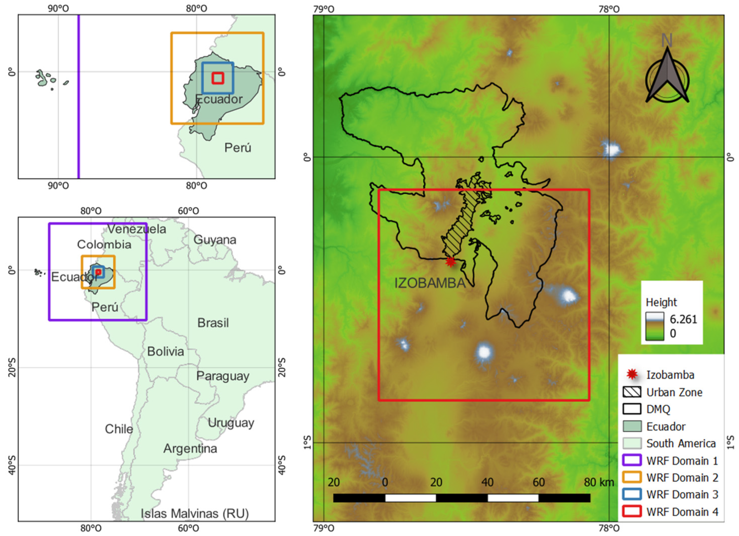
2. Study Area
3. Data and Methods
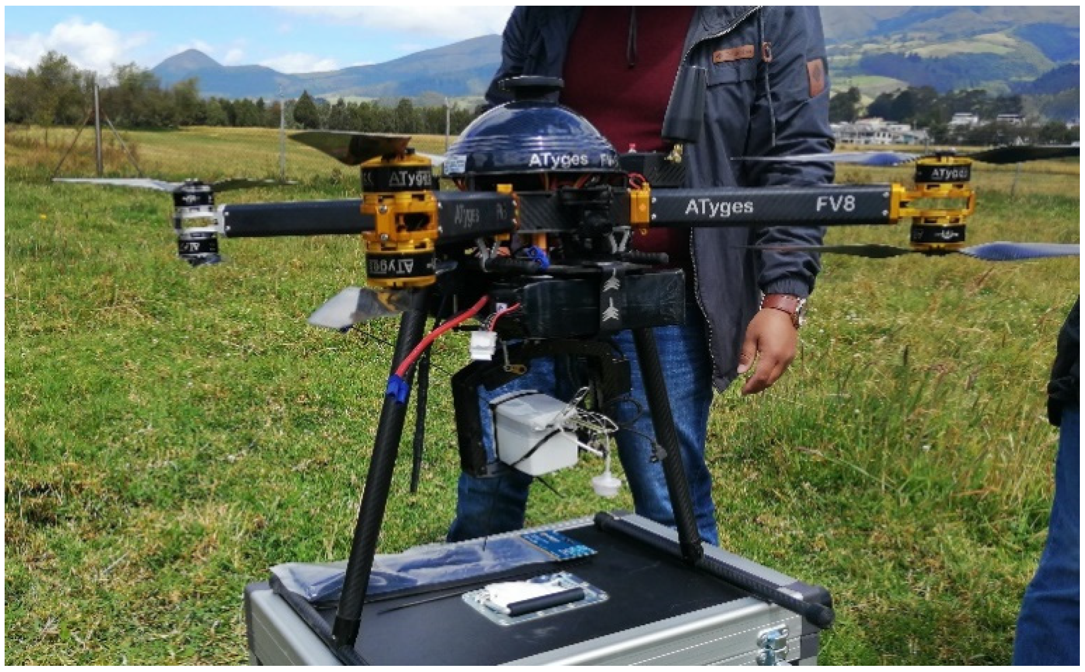
3.1. Radiosonde and Drone Data
3.2. Satellite Data
3.3. WRF Data, Parametrizations, and Processing
3.4. Results Evaluation
3.5. hPBL Calculation Methods
4. Results and Discussion
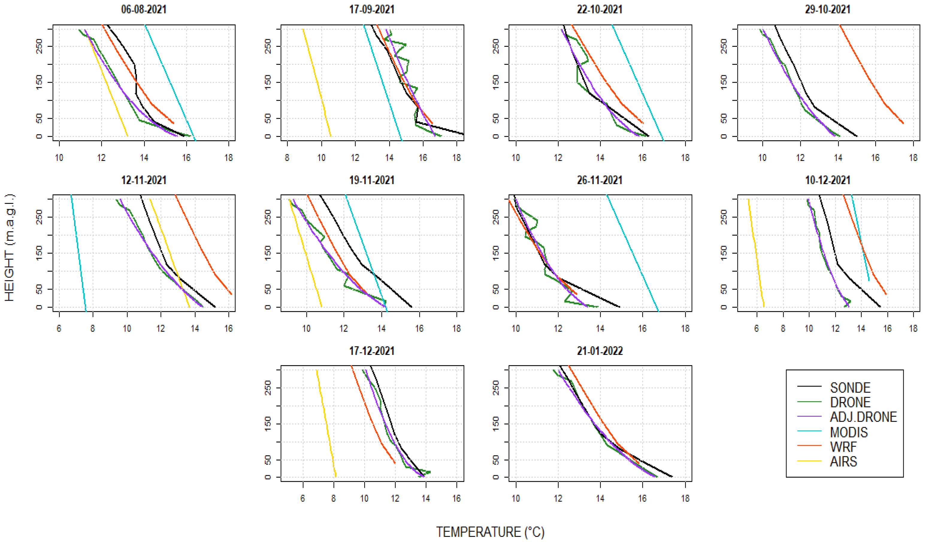
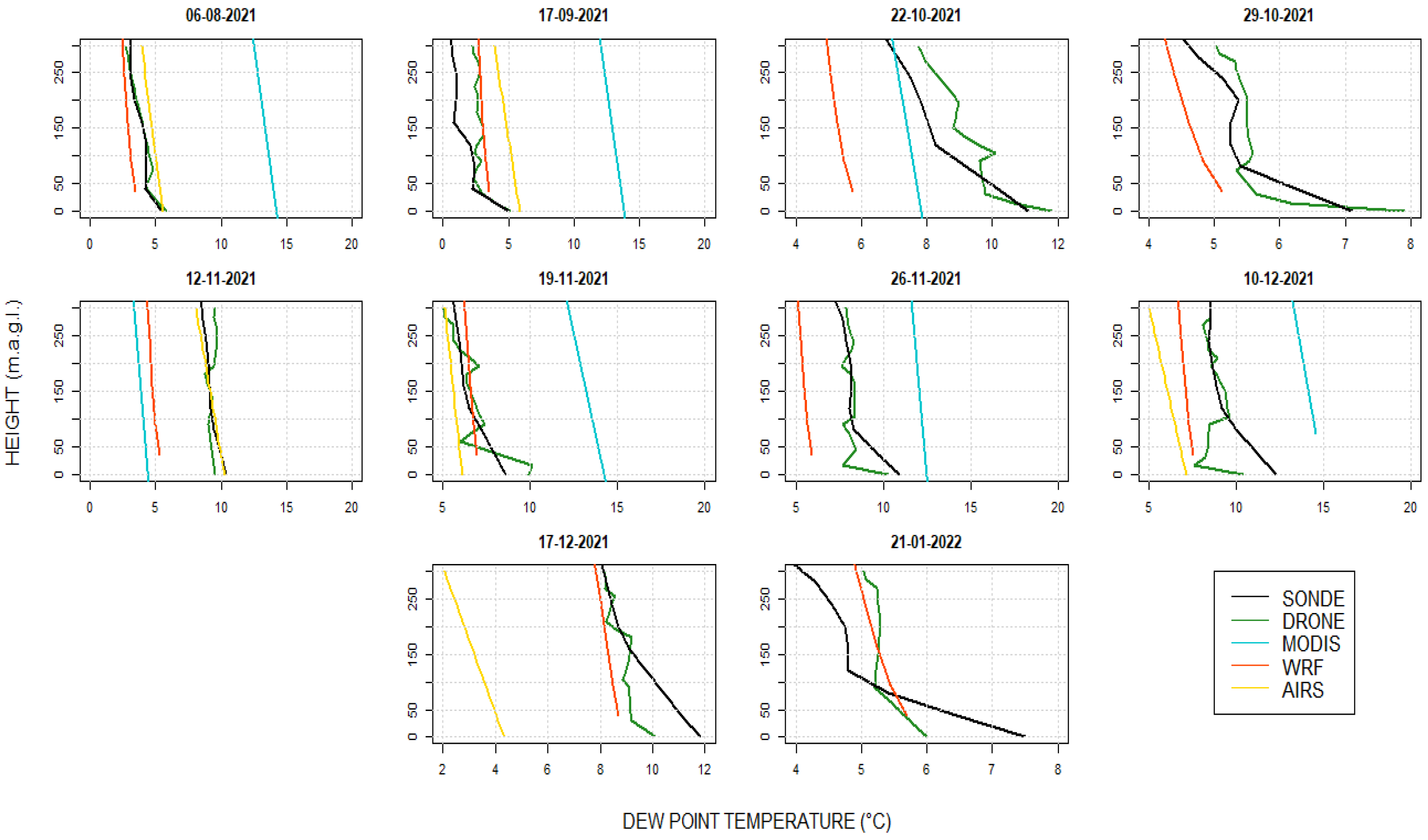
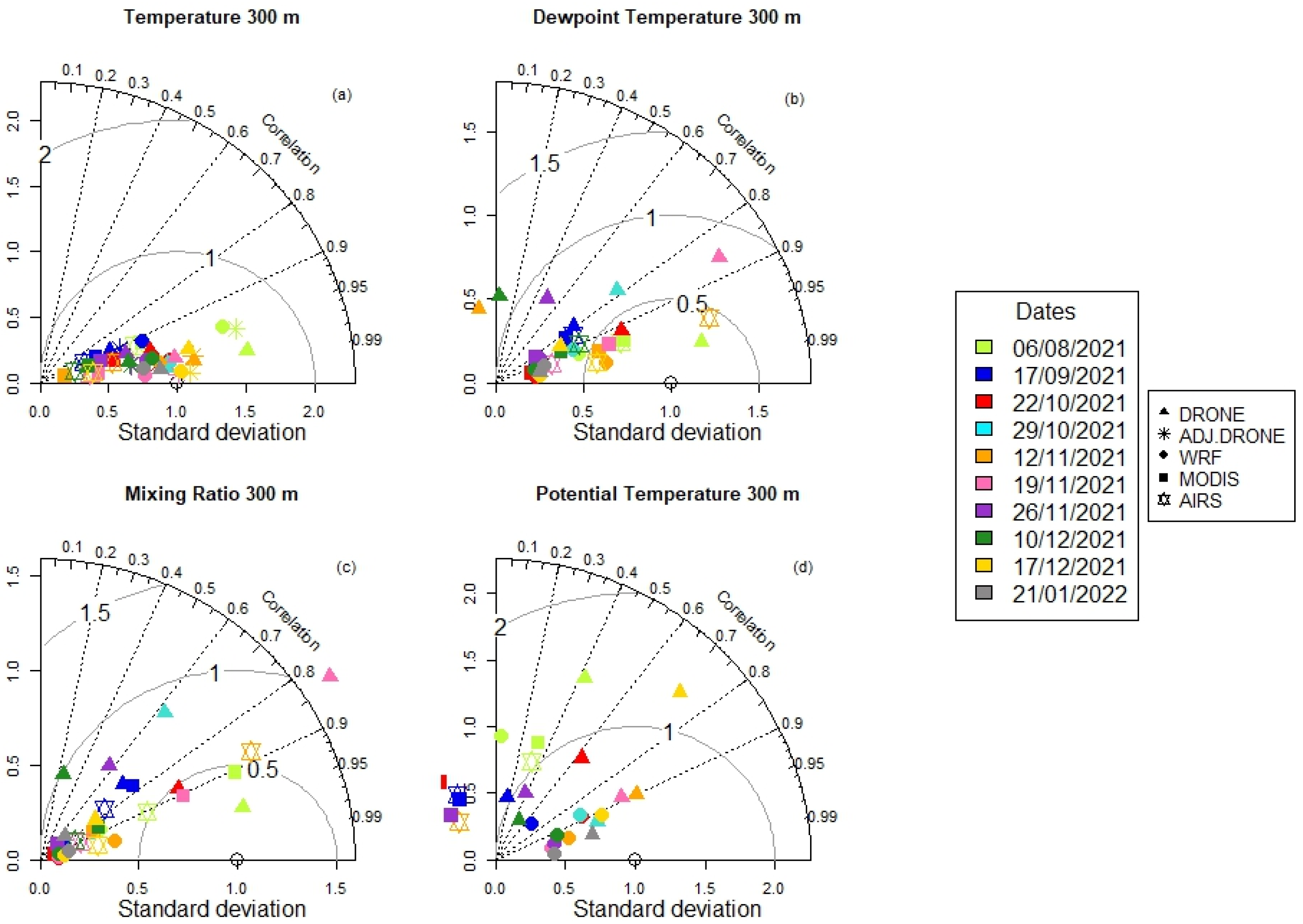
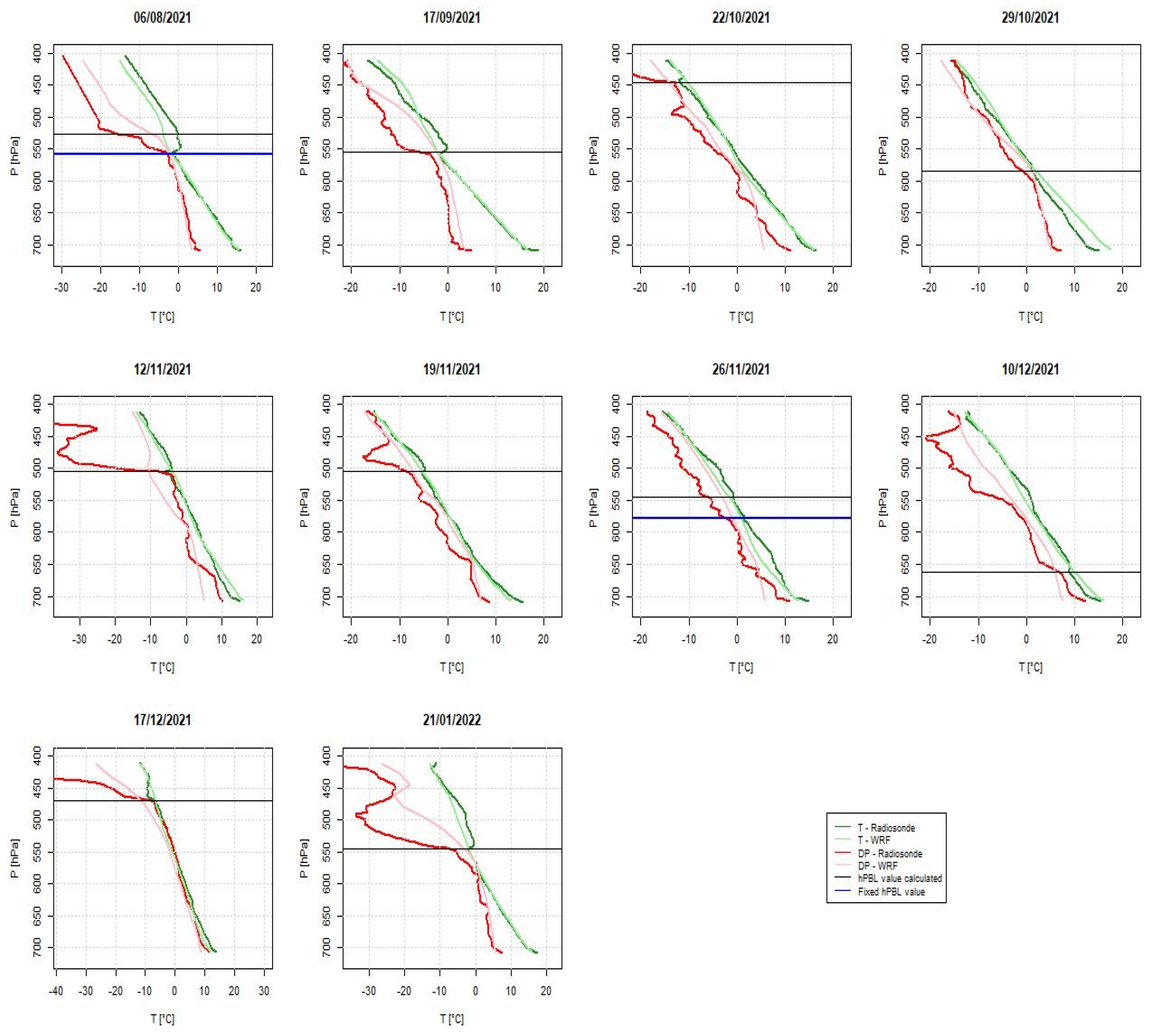
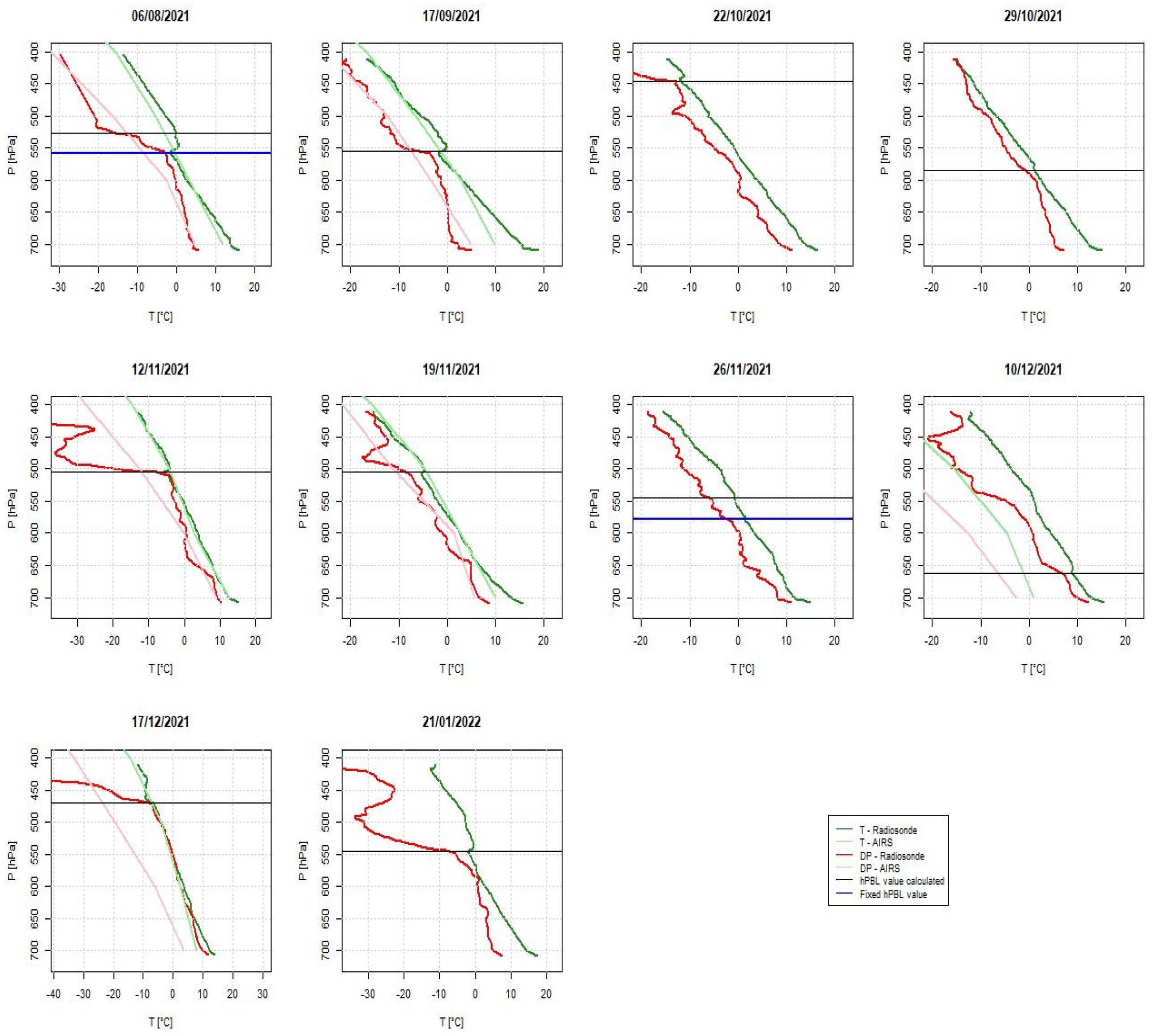
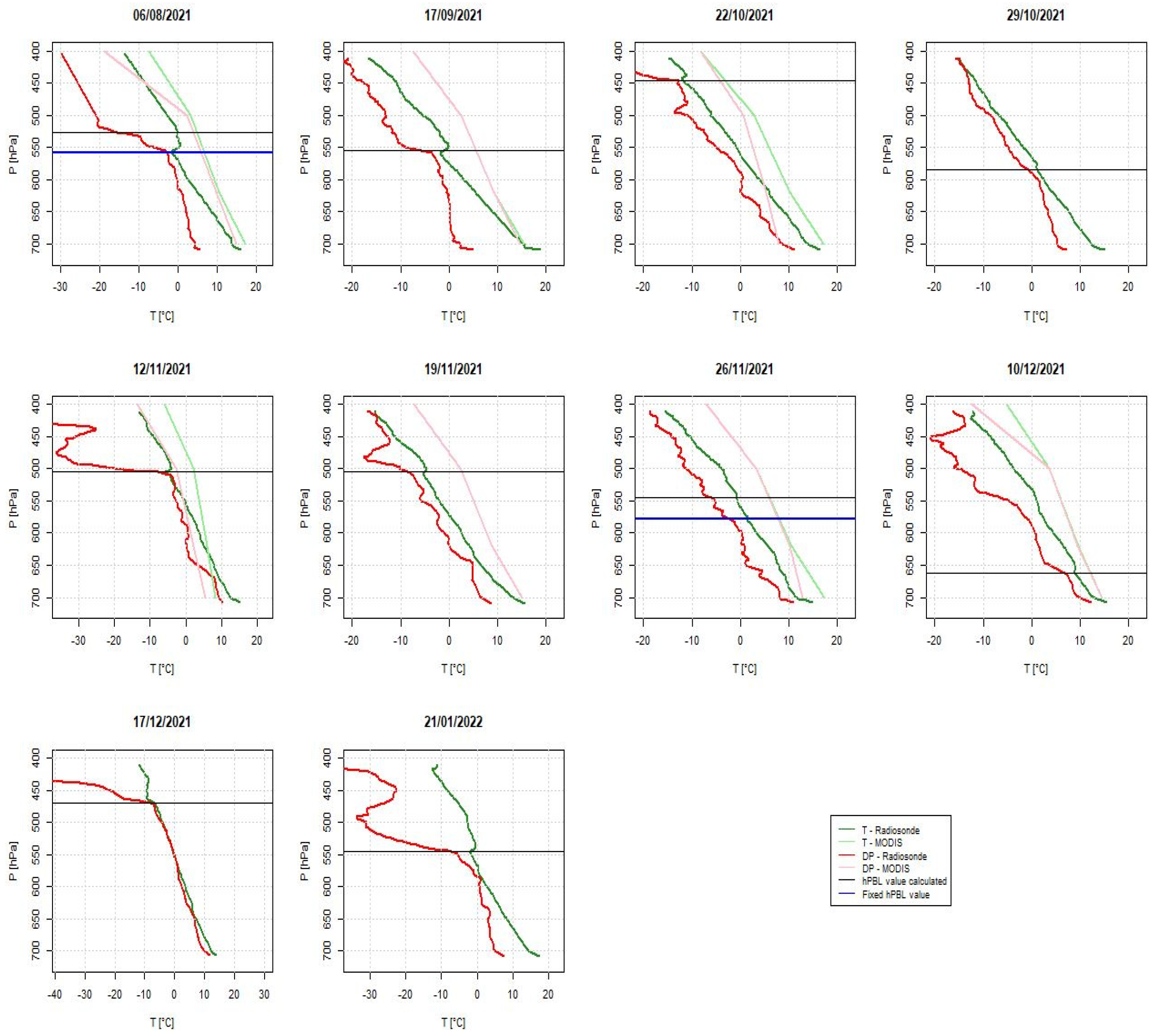
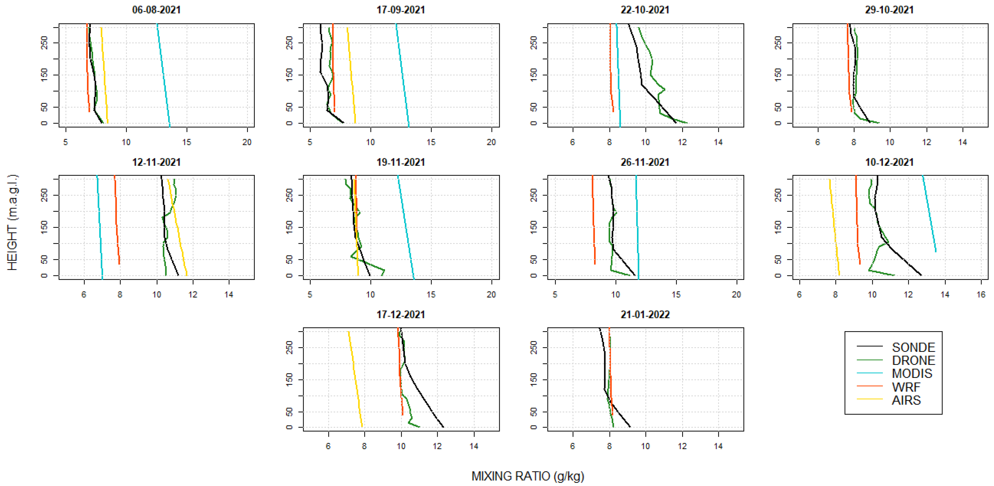
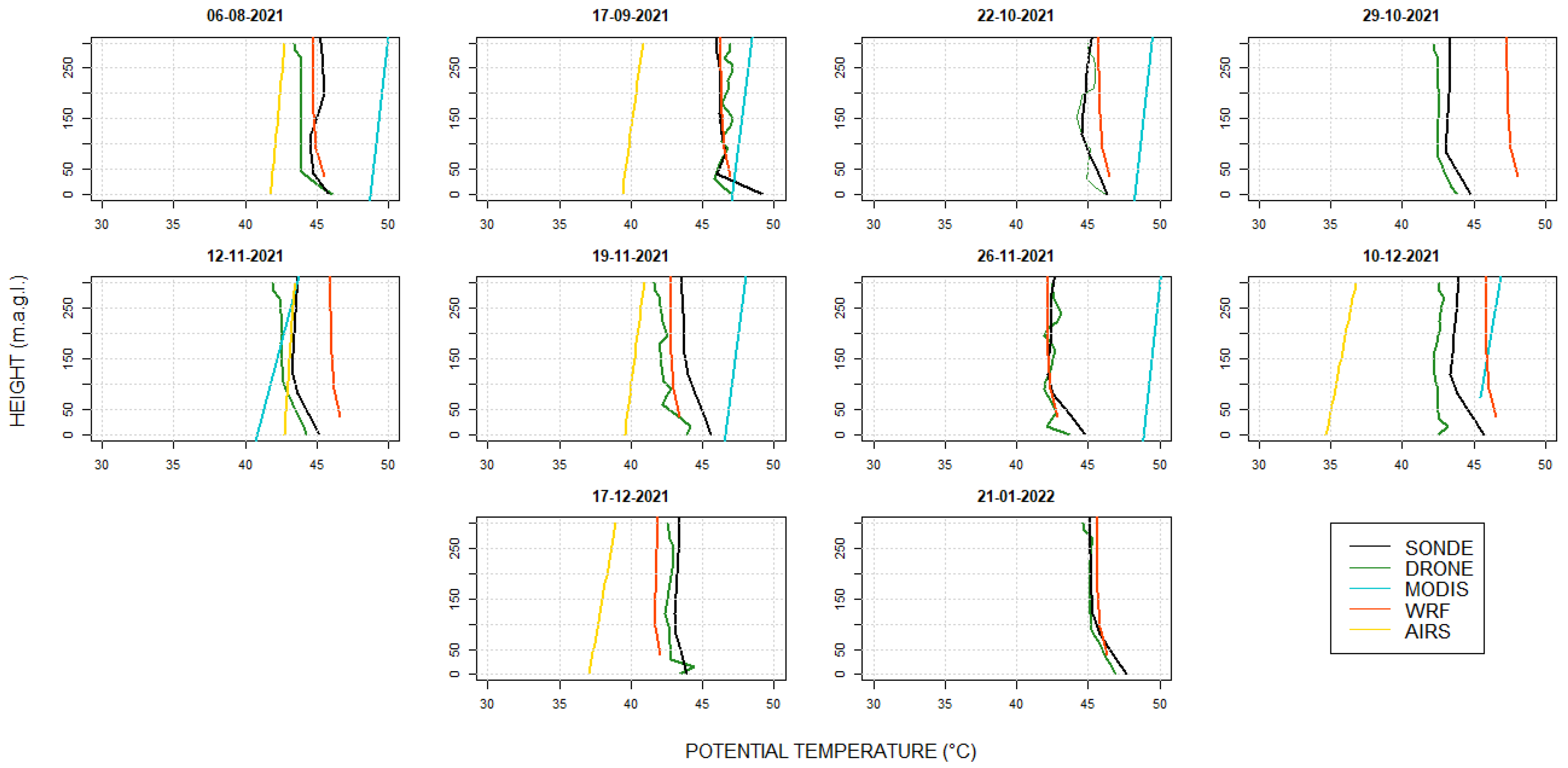
4.1. Lower Troposphere Analysis
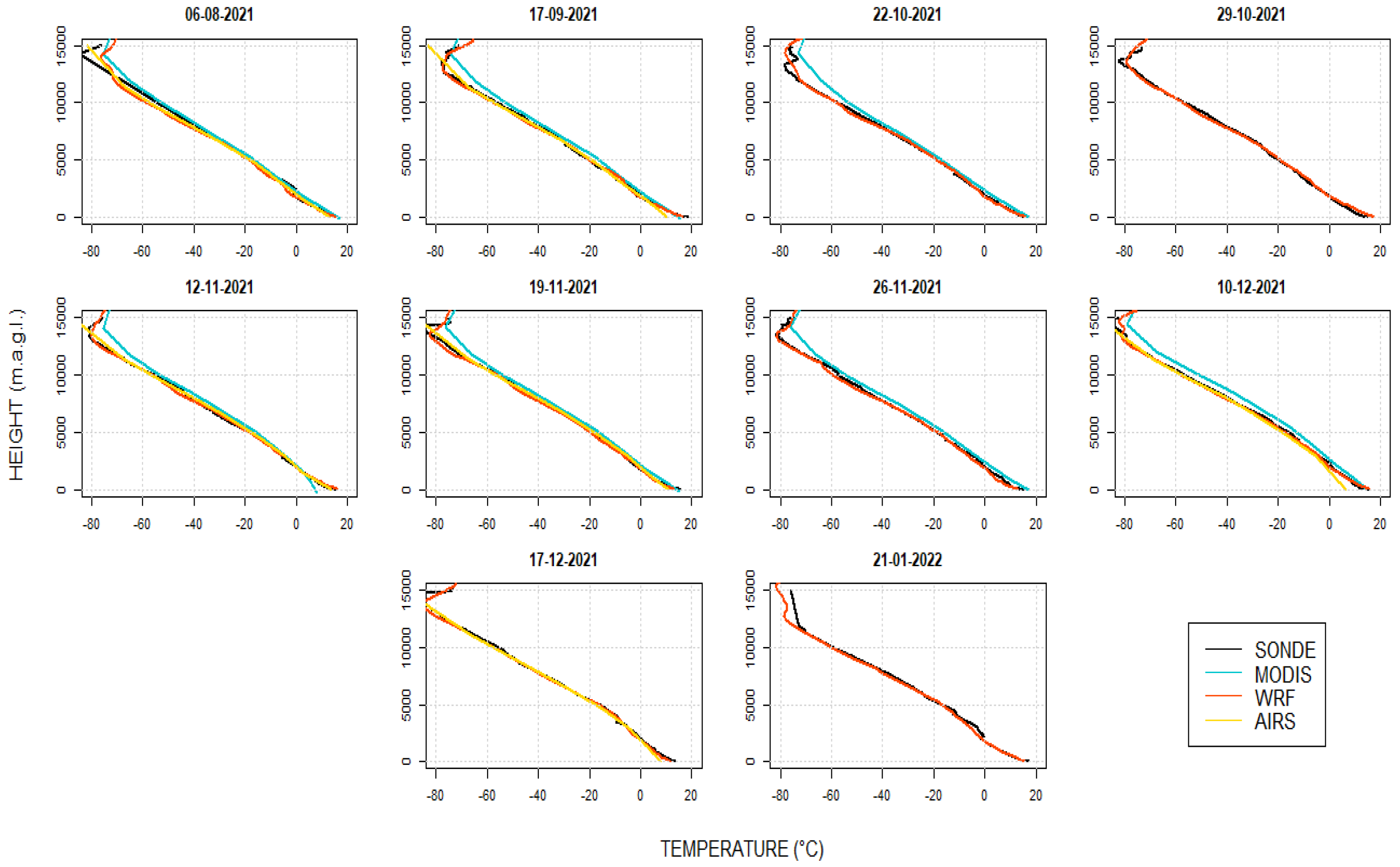
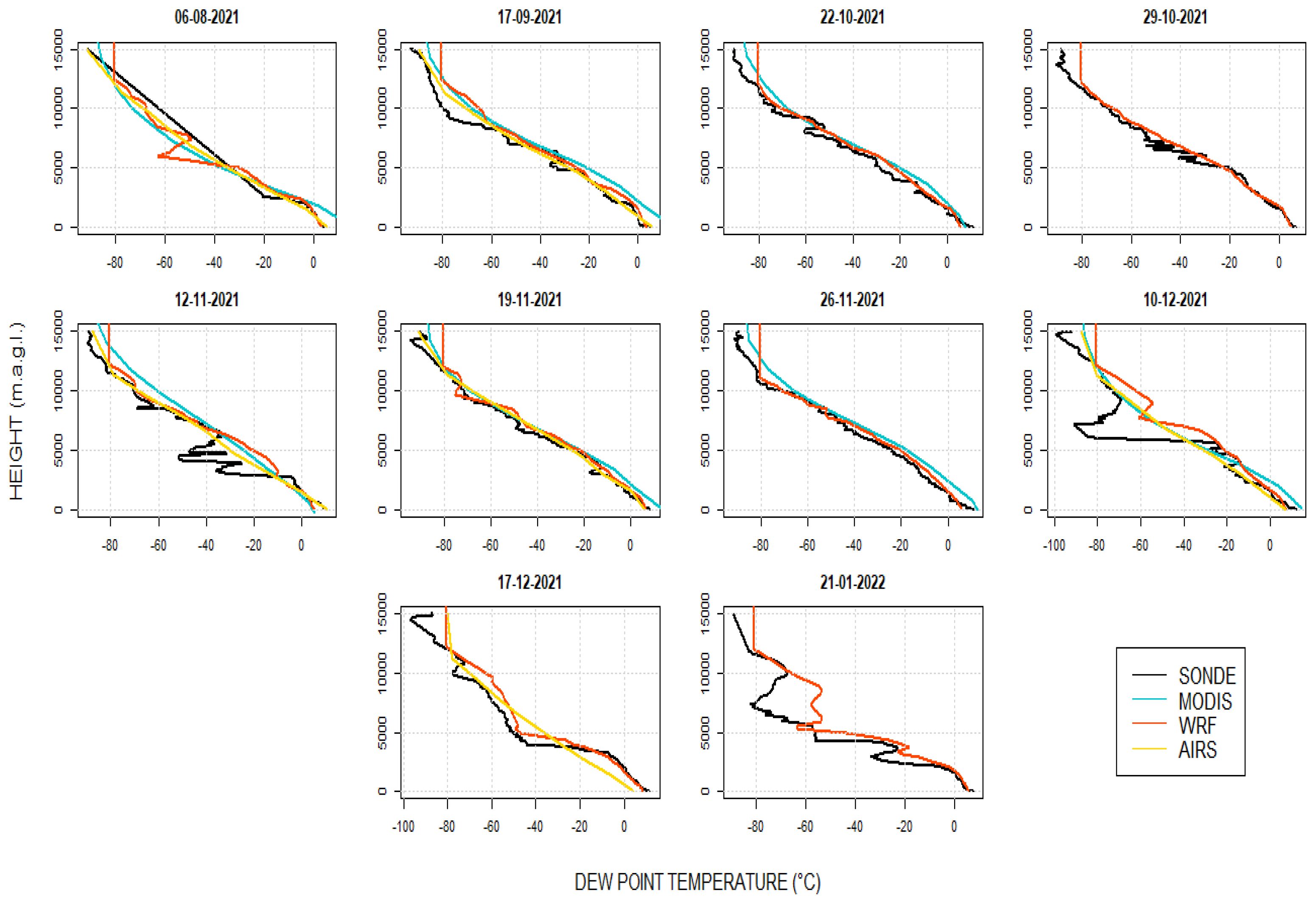
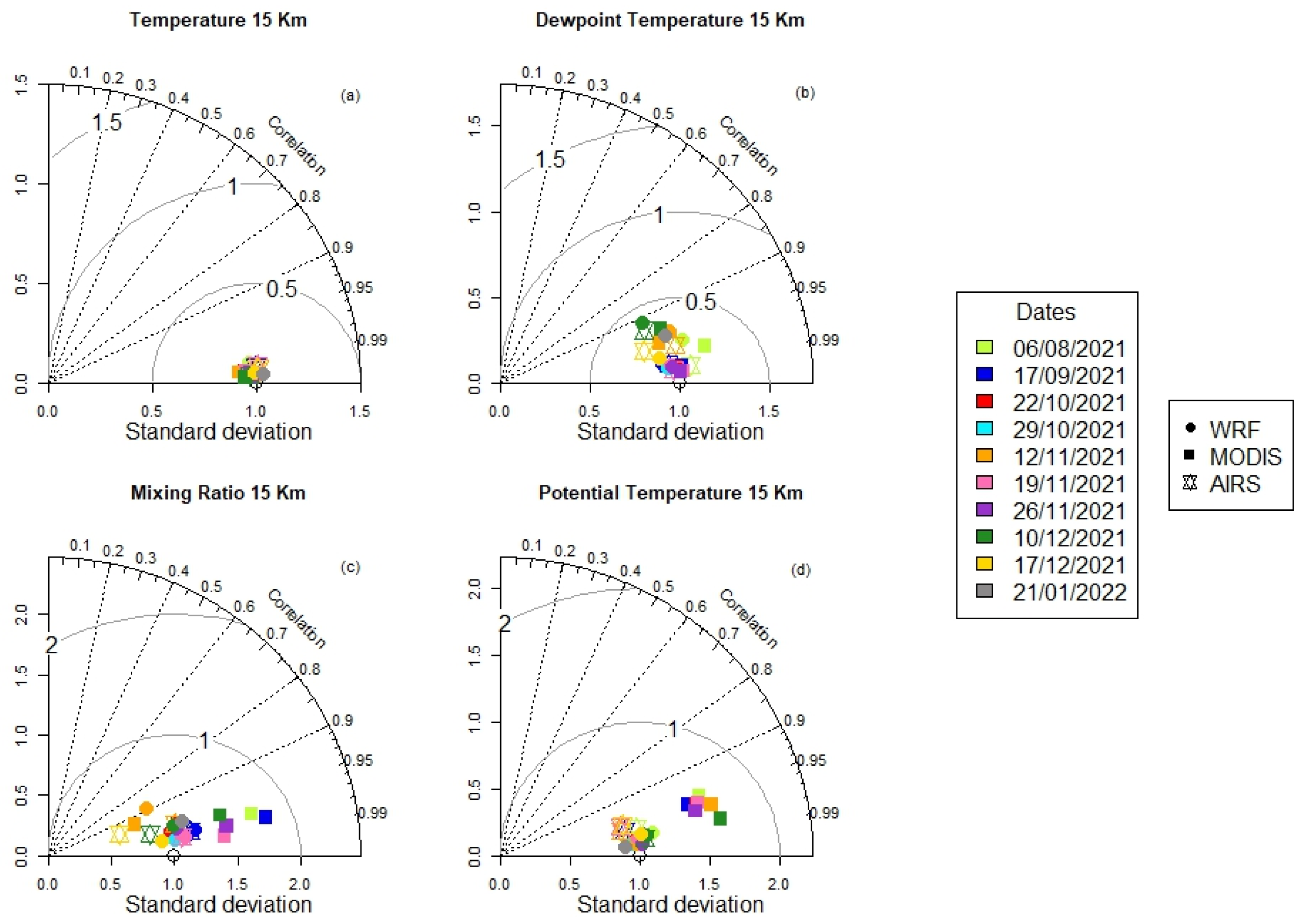
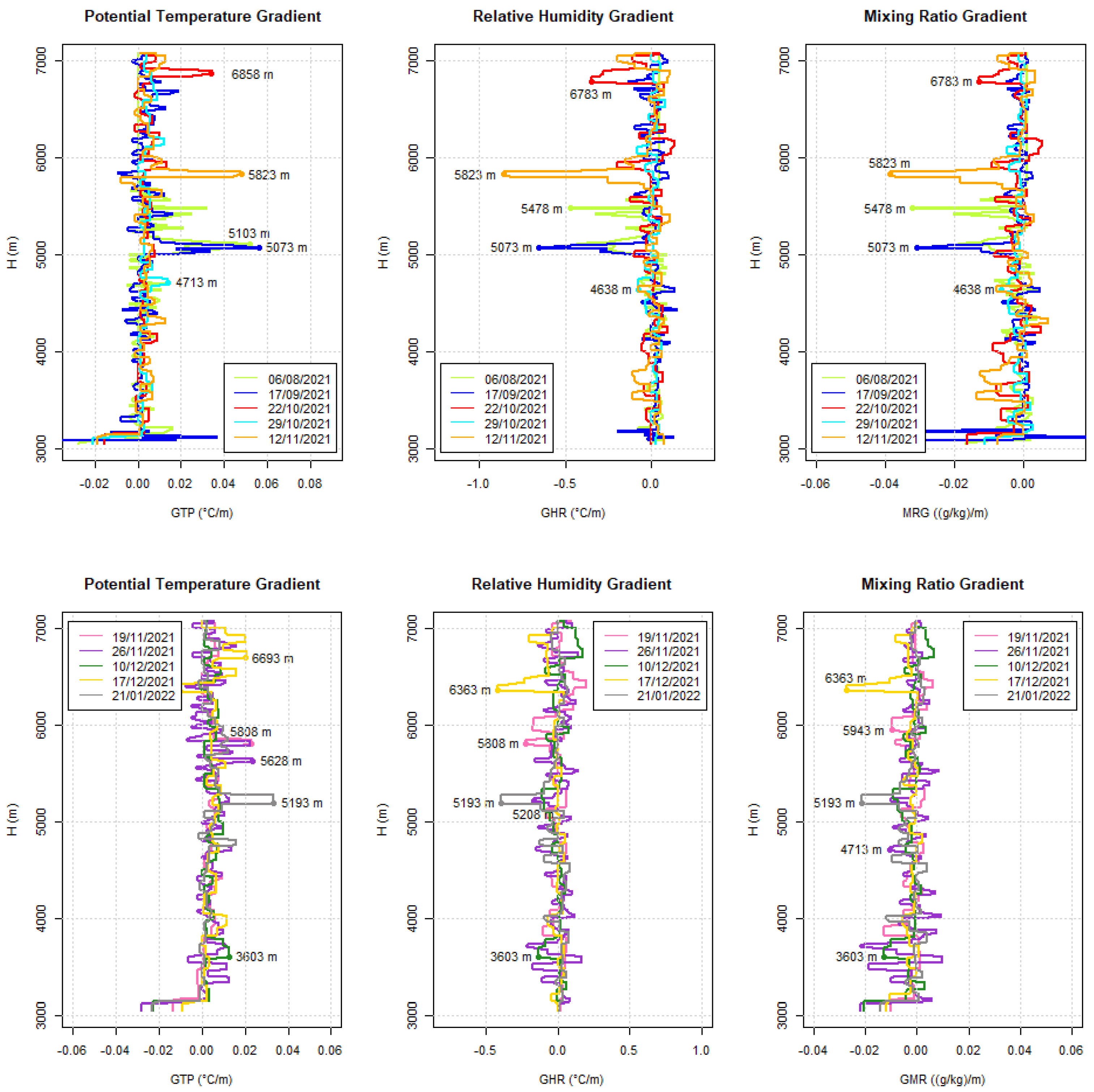
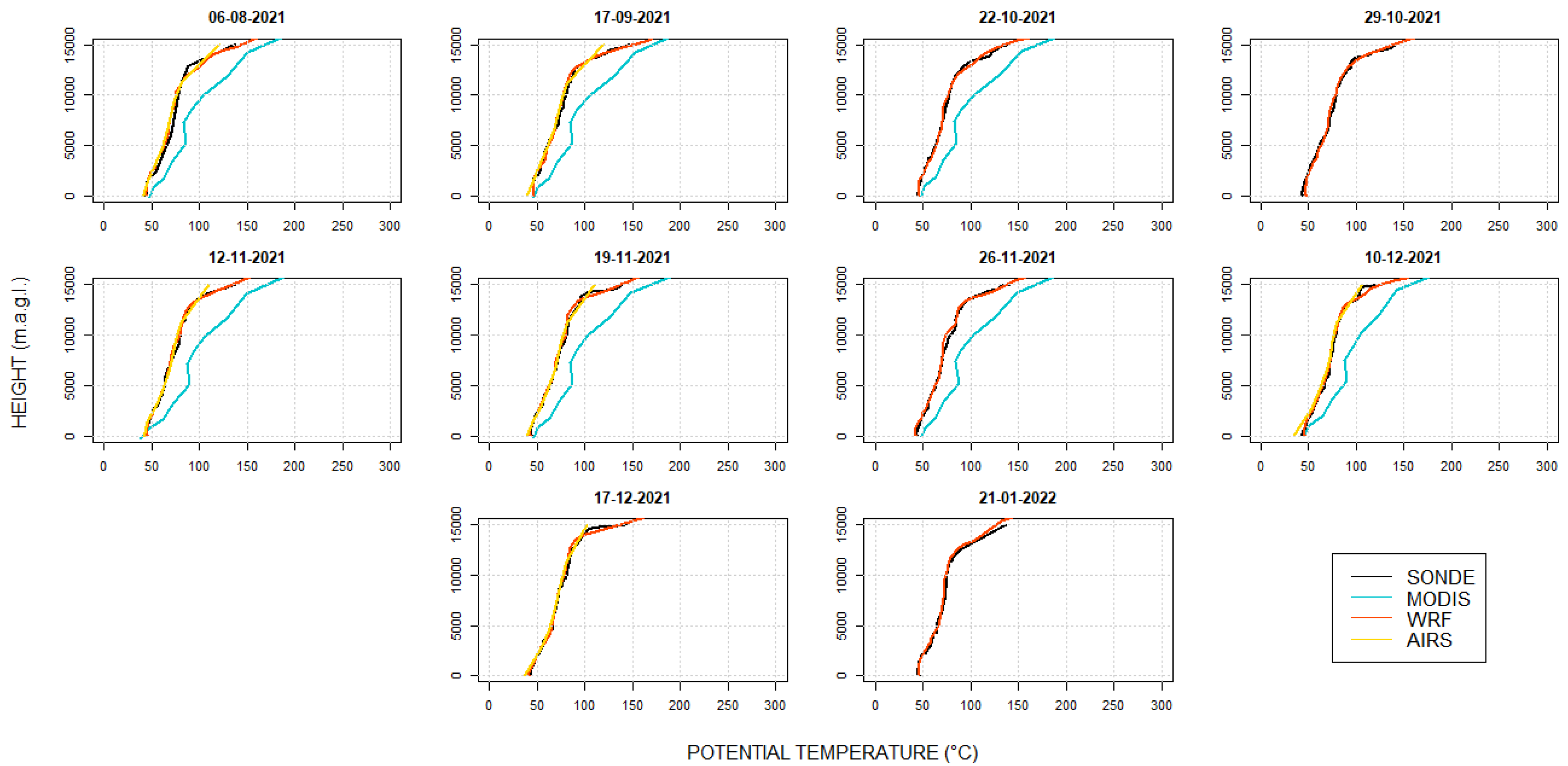
4.2. Upper Troposphere Analysis
4.3. hPBL Analysis
5. Concluding Remarks
Author Contributions
Funding
Institutional Review Board Statement
Informed Consent Statement
Data Availability Statement
Acknowledgments
Conflicts of Interest
Appendix A
Appendix A.1

Appendix A.2

Appendix A.3

Appendix A.4

Appendix A.5

References
- Thorne, P.W.; Allan, R.J.; Ashcroft, L.; Brohan, P.; Dunn, R.J.H.; Menne, M.J.; Pearce, P.R.; Picas, J.; Willett, K.M.; Benoy, M.; et al. Toward an integrated set of surface meteorological observations for climate science and applications. Bull. Am. Meteorol. Soc. 2017, 98, 2689–2702. [Google Scholar] [CrossRef]
- World Meteorological Organization (WMO). Guide to instruments and methods of observation. In Guide to Instruments and Methods of Observation; Vols. I & II; WMO: Geneva, Switzerland, 2018. [Google Scholar]
- Estévez, J.; Gavilán, P.; Giráldez, J.V. Guidelines on Validation Procedures for Meteorological Data from Automatic Weather Stations. J. Hydrol. 2011, 402, 144–154. [Google Scholar] [CrossRef]
- Bayer, A.; van Iersel, M.; Chappell, M. What Is a weather station, and can it benefit ornamental growers? UGA Coop. Ext. Bull. 2017, 1475, 6. [Google Scholar]
- Li, C.; Sun, X. A novel meteorological sensor data acquisition approach based on unmanned aerial vehicle. Int. J. Sens. Netw. 2018, 28, 80–88. [Google Scholar] [CrossRef]
- Lopes, I.; Guimarães, M.J.M.; de Melo, J.M.M.; de Almeida, C.D.G.C.; Lopes, B.; Leal, B.G. Comparison of meteorological data, related to reference evapotranspiration, from conventional and automatic stations in the Sertão and Agreste Regions of Pernambuco, Brazil. DYNA 2021, 88, 176–183. [Google Scholar] [CrossRef]
- Seidel, D.J.; Ao, C.O.; Li, K. Estimating climatological planetary boundary layer heights from radiosonde observations: Comparison of methods and uncertainty analysis. J. Geophys. Res. Atmos. 2010, 115, 1–15. [Google Scholar] [CrossRef]
- Sivaraman, C.; Mcfarlane, S.; Chapman, E.; Jensen, M.; Toto, T.; Lui, S.; Fischer, M. Planetary Boundary Layer (PBL) Height Value Added Product (VAP): Radiosonde Retrievals. In Climate Research Facility; U.S. Department of Energy: Washington, DC, USA, 2013; Volume 1. [Google Scholar]
- Cazorla, M.; Juncosa, J. Planetary boundary layer evolution over an equatorial Andean Valley: A simplified model based on balloon-borne and surface measurements. Atmos. Sci. Lett. 2018, 19, e829. [Google Scholar] [CrossRef]
- Villa, T.F.; Gonzalez, F.; Miljievic, B.; Ristovski, Z.; Morawska, L. An overview of small unmanned aerial vehicles for air quality measurements: Present applications and future prospectives. Sensors 2016, 16, 1072. [Google Scholar] [CrossRef] [PubMed]
- Wang, Y.C.; Wang, S.H.; Lewis, J.R.; Chang, S.C.; Griffith, S.M. Determining planetary boundary layer height by micro-pulse lidar with validation by UAV measurements. Aerosol Air Qual. Res. 2021, 21, 200336. [Google Scholar] [CrossRef]
- Masot, A.N.; García, C.; Fernández, A. Aplicaciones de los satélites Meteosat y MODIS para discriminar fenómenos naturales: Detección de incendios y puntos calientes, evolución de borrascas, ciclogénesis explosiva y cenizas volcánicas. In Congreso Nacional de Tecnologías de la Información Geográfica; Universidad de Sevilla: Seville, Spain, 2010; pp. 942–955. [Google Scholar]
- Molero, F.; Barragán, R.; Artíñano, B. Estimation of the atmospheric boundary layer height by means of machine learning techniques using ground-level meteorological data. Atmos. Res. 2022, 279, 106401. [Google Scholar] [CrossRef]
- Zhang, D.; Comstock, J.; Morris, V. Comparison of planetary boundary layer height from ceilometer with ARM radiosonde data. Atmos. Meas. Tech. 2022, 15, 4735–4749. [Google Scholar] [CrossRef]
- Adamo, M.; de Carolis, G.; Morelli, S. Comparison of MODIS and ETA profiles of atmospheric parameters in coastal zones with radiosonde data. Nuovo Cim. Della Soc. Ital. Fis. C 2007, 30, 255–275. [Google Scholar] [CrossRef]
- Pérez-Planells, L.; García-Santos, V.; Caselles, V. Comparing different profiles to characterize the atmosphere for three MODIS TIR bands. Atmos. Res. 2015, 161–162, 108–115. [Google Scholar] [CrossRef]
- Feng, X.; Wu, B.; Yan, N. A method for Deriving the Boundary Layer Mixing Height from MODIS Atmospheric Profile Data. Atmosphere 2015, 6, 1346–1361. [Google Scholar] [CrossRef]
- Onyango, S.; Anguma, S.K.; Andima, G.; Parks, B. Validation of the atmospheric boundary Layer Height Estimated from the MODIS Atmospheric Profile Data at an Equatorial Site. Atmosphere 2020, 11, 908. [Google Scholar] [CrossRef]
- Feng, X.; Tang, L.; Han, G.; Chen, W. Temperature Gradient Method for Deriving Planetary Boundary Layer Height from AIRS Profile Data over the Heihe River Basin of China. Arab. J. Geosci. 2021, 14, 87. [Google Scholar] [CrossRef]
- Ding, F.; Iredell, L.; Theobald, M.; Wei, J.; Meyer, D. PBL height from AIRS, GPS RO, and MERRA-2 products in NASA GES DISC and their 10-year seasonal mean intercomparison. Earth Space Sci. 2021, 8, e2021EA001859. [Google Scholar] [CrossRef]
- Martins, J.P.A.; Teixeira, J.; Soares, P.M.M.; Miranda, P.M.A.; Kahn, B.H.; Dang, V.T.; Irion, F.W.; Fetzer, E.J.; Fishbein, E. Infrared sounding of the trade-wind boundary layer: AIRS and the RICO experiment. Geophys. Res. Lett. 2010, 37, L24806. [Google Scholar] [CrossRef]
- Caneo, M.; Pozo, D.; Illanes, L.; Curé, M. A comparison between sounding data and WRF forecasts at APEX site. Rev. Mex. Astron. Astrofis. Conf. 2011, 41, 59–62. [Google Scholar]
- Fekih, A.; Mohamed, A. Evaluation of the WRF model on simulating the vertical structure and diurnal cycle of the atmospheric boundary layer over Bordj Badji Mokhtar (southwestern Algeria). J. King Saud. Univ. Sci. 2019, 31, 602–611. [Google Scholar] [CrossRef]
- Parra, R. Assessment of planetary boundary layer schemes of the WRF-CHEM model in the simulation of carbon monoxide dispersion in the urban area of Quito, Ecuador. WIT Trans. Ecol. Environ. 2017, 211, 41–50. [Google Scholar] [CrossRef]
- Parra, R. Performance studies of planetary boundary layer schemes in WRF-Chem for the Andean region of Southern Ecuador. Atmos. Pollut. Res. 2018, 9, 411–428. [Google Scholar] [CrossRef]
- García-Gutiérrez, A.; Domínguez, D.; López, D.; Gonzalo, J. Atmospheric boundary layer wind profile estimation using neural networks applied to lidar measurements. Sensors 2021, 21, 3659. [Google Scholar] [CrossRef] [PubMed]
- Rieutord, T.; Aubert, S.; Machado, T. Deriving boundary layer height from aerosol lidar using machine learning: KABL and ADABL algorithms. Atmos. Meas. Tech. 2021, 14, 4335–4353. [Google Scholar] [CrossRef]
- Korolkov, V.A.; Pustovalov, K.N.; Tikhomirov, A.A.; Telminov, A.E.; Kurakov, S.A. Autonomous weather stations for unmanned aerial vehicles. Preliminary results of measurements of meteorological profiles. IOP Conf. Ser. Earth Environ. Sci. 2018, 211, 012069. [Google Scholar] [CrossRef]
- Laitinen, A. Utilization of Drones in Vertical Profile Measurements of the Atmosphere; Tampere University: Tampere, Finland, 2019; Available online: http://urn.fi/URN:NBN:fi:tuni-201907252745 (accessed on 17 August 2021).
- Novotný, J.; Bystrický, R.; Dejmal, K. Meteorological application of UAV as a new way of vertical profile of lower atmosphere measurement. Chall. Natl. Def. in Contemp. Geopolit. Situat. 2018, 2018, 115–120. [Google Scholar] [CrossRef]
- Basha, G.; Ratnam, M.V. Identification of atmospheric boundary layer height over a tropical station using high-resolution radiosonde refractivity profiles: Comparison with GPS radio occupation measurements. J. Geophys. Re. Atmos. 2009, 114, 1–11. [Google Scholar] [CrossRef]
- Shikhovtsev, A.Y. A method of determining optical turbulence characteristics by the line of sight of an astronomical telescope. Atmos. Ocean. Opt. 2022, 35, 303–309. [Google Scholar] [CrossRef]
- Shikhovtsev, A.Y.; Kovadlo, P.G.; Khaikin, V.B.; Nosov, V.V.; Lukin, V.P.; Nosov, E.V.; Torgaev, A.V.; Kiselev, A.V.; Shikhovtsev, M.Y. Atmospheric conditions within big telescope Alt-Azimuthal Region and possibilities of astronomical observations. Remote Sens. 2022, 14, 1833. [Google Scholar] [CrossRef]
- Zhang, J.; Guo, J.; Li, J.; Zhang, S.; Tong, B.; Shao, J.; Li, H.; Zhang, Y.; Cao, L.; Zhai, P.; et al. A climatology of merged daytime planetary boundary layer height over China from radiosonde measurements. J. Geophys. Res. Atmos. 2022, 127, e2021JD036367. [Google Scholar] [CrossRef]
- Vicente-Serrano, S.M.; Aguilar, E.; Martínez, R.; Martín-Hernández, N.; Azorin-Molina, C.; Sanchez-Lorenzo, A.; el Kenawy, A.; Tomás-Burguera, M.; Moran-Tejeda, E.; López-Moreno, J.I.; et al. The complex influence of ENSO on droughts in Ecuador. Clim. Dyn. 2017, 48, 405–427. [Google Scholar] [CrossRef]
- Campozano, L.; Trachte, K.; Célleri, R.; Samaniego, E.; Bendix, J.; Albuja, C.; Mejia, J.F. Climatology and teleconnections of mesoscale convective systems in an Andean Basin in Southern Ecuador: The case of the Paute Basin. Adv. Meteorol. 2018, 2018, 4259191. [Google Scholar] [CrossRef]
- Serrano-Vicenti, S.; Zuleta, D.; Moscoso, V.; Jácome, P.; Palacios, E.; Villacís, M. Análisis estadístico de datos meteorológicos mensuales y diarios para la determinación de variabilidad climática y cambio climático en el Distrito Metropolitano de Quito. La Granja 2012, 16, 23–47. [Google Scholar] [CrossRef]
- Campozano, L.; Célleri, R.; Trachte, K.; Bendix, J.; Samaniego, E. Rainfall and cloud dynamics in the Andes: A Southern Ecuador Case Study. Adv. Meteorol. 2016, 2016, 3192765. [Google Scholar] [CrossRef]
- Serrano, S.; Zuleta, D.; Moscoso, V.; Jácome, P.; Palacios, E.; Villacís, M. Statistical analysis of daily and monthly meteorological data of the Metropolitan District of Quito for weather variability and climate change studies. La Granja 2012, 16, 23–47. [Google Scholar]
- Llugsi, R.; Fontaine, A.; Lupera, P.; Bechet, J.; el Yacoubi, S. Uncertainty reduction in the neural network’s weather forecast for the Andean city of Quito through the adjustment of the posterior predictive distribution based on estimators. In Information and Communication Technologies; Springer: Cham, Switzerland, 2020; Volume 1307, pp. 535–548. [Google Scholar] [CrossRef]
- Serrano-Vincenti, S.; Ruiz, J.C.; Bersosa, F. Heavy rainfall and temperature projections in a climate change scenario over Quito, Ecuador. La Granja 2016, 25, 16. [Google Scholar] [CrossRef]
- Vaisala Vaisala Radiosonde RS92-SGP Datasheet. 2013. Available online: www.vaisala.com (accessed on 8 July 2022).
- Rodriguez, O.; Arredondo, H. Manual Para el Manejo y Procesamiento de Imágenes Satelitales Obtenidas del Sensor Remoto MODIS de la NASA, Aplicado en Estudios de Ingeniería Civil; Pontificia Universidad Javeriana: Bogotá, Colombia, 2005; Available online: https://repository.javeriana.edu.co/bitstream/handle/10554/7050/tesis123.pdf?sequence=3&isAllowed=y (accessed on 18 September 2022).
- Reymondin, L. The benefits of MODIS. Available online: http://www.terra-i.org/news/news/The-benefits-of-MODIS.html (accessed on 23 September 2021).
- Weather Spark El Clima y El Tiempo Promedio En Todo El Año En Quito, Ecuador. Available online: https://es.weatherspark.com/y/20030/Clima-promedio-en-Quito-Ecuador-durante-todo-el-a%C3%B1o#Sections-Clouds (accessed on 29 April 2022).
- Thrastarson, H.; Fetzer, E.; Ray, S. Overview of the AIRS Mission: Instruments, Processing Algorithms, Products, and Documentation; Jet Propulsion Laboratory California Institute of Technology: Pasadena, CA, USA, 2021. Available online: https://airs.jpl.nasa.gov/data/support/ask-airs (accessed on 31 October 2022).
- The HDF Group HDF-EOS to GeoTIFF Conversion Tool (HEG). Available online: https://hdfeos.org/software/heg.php (accessed on 24 November 2022).
- AIRS project. Aqua/AIRS L2 Standard Physical Retrieval (AIRS-Only) V7.0.; Goddard Earth Sciences Data and Information Services Center (GES-DISC): Greenbelt, MD, USA, 2019. Available online: https://disc.gsfc.nasa.gov/datasets/AIRS2RET_7.0/summary?keywords=aIRS (accessed on 20 September 2022).
- Heredia, M.B.; Junquas, C.; Prieur, C.; Condom, T. New Statistical Methods for Precipitation Bias Correction Applied to WRF Model Simulations in the Antisana Region, Ecuador. J. Hydrometeorol. 2018, 19, 2021–2040. [Google Scholar] [CrossRef]
- Skamarock, W.C.; Klemp, J.B.; Dudhia, J.; Gill, D.O.; Zhiquan, L.; Berner, J.; Wang, W.; Powers, J.G.; Duda, M.G.; Barker, D.M.; et al. A description of the advanced research WRF Model Version 4. In NCAR Technical Note NCAR/TN475+STR; NCAR: Boulder, CO, USA, 2019; Available online: http://library.ucar.edu/research/publish-technote (accessed on 19 March 2022).
- Ochoa, A.; Campozano, L.; Sánchez, E.; Gualán, R.; Samaniego, E. Evaluation of downscaled estimates of monthly temperature and precipitation for a Southern Ecuador case study. Int. J. Climatol. 2016, 36, 1244–1255. [Google Scholar] [CrossRef]
- Xu, J.; Rugg, S.; Byerle, L.; Liu, Z. Weather Forecasts by the WRF-ARW Model with the GSI Data Assimilation System in the complex terrain areas of Southwest Asia. Weather Forecast. 2009, 24, 987–1008. [Google Scholar] [CrossRef]
- Mourre, L.; Condom, T.; Junquas, C.; Lebel, T.; Sicart, J.E.; Figueroa, R.; Cochachin, A. Spatio-temporal assessment of WRF, TRMM and in situ precipitation data in a tropical mountain environment (Cordillera Blanca, Peru). Hydrol. Earth Syst. Sci. 2016, 20, 125–141. [Google Scholar] [CrossRef]
- Junquas, C.; Takahashi, K.; Condom, T.; Espinoza, J.C.; Chavez, S.; Sicart, J.E.; Lebel, T. Understanding the influence of orography on the precipitation diurnal cycle and the associated atmospheric processes in the central Andes. Clim. Dyn. 2018, 50, 3995–4017. [Google Scholar] [CrossRef]
- Parra, R.; Cadena, E.; Paz, J.; Medina, D. Isomass and probability maps of ash fallout due to vulcanian eruptions at Tungurahua Volcano (Ecuador) deduced from historical forecasting. Atmosphere. 2020, 11, 861. [Google Scholar] [CrossRef]
- Schuyler, T.J.; Gohari, S.M.I.; Pundsack, G.; Berchoff, D.; Guzman, M.I. Using a balloon-launched unmanned glider to validate real-time WRF modeling. Sensors 2019, 19, 1914. [Google Scholar] [CrossRef] [PubMed]
- ARW OnLine Tutorial Nested Model Runs. 2018. Available online: https://www2.mmm.ucar.edu/wrf/OnLineTutorial/CASES/NestRuns/2way2inputs.htm (accessed on 4 January 2021).
- WRF Users Page. WRF Users’ Guide. Available online: https://www2.mmm.ucar.edu/wrf/users/docs/user_guide_V3.9/contents.html (accessed on 6 December 2020).
- National Centers for Environmental Prediction (NCEP); National Weather Service; National Oceanic and Atmospheric Administration (NOAA); U.S. Department of Commerce. NCEP FNL Operational Model Global Tropospheric Analyses, Continuing from July 1999; Research Data Archive at the National Center for Atmospheric Research, Computational and Information Systems Laboratory; UCAR: Boulder, CO, USA, 2000; Available online: https://rda.ucar.edu/datasets/ds083.2/ (accessed on 30 April 2022).
- Davydova-Belitskaya, V.; Rosario de la Cruz, J.; Rodríguez-López, O. Un modelo de verificación de pronósticos de precipitación. Ingeniería 2017, 20, 24–33. [Google Scholar]
- López, L. Evaluación de la calidad del pronóstico numérico del tiempo en la Ciudad de México. Ph.D. Thesis, Universidad Nacional Autónoma de México, Mexico City, Mexico, 2012. Available online: https://dspace.ups.edu.ec/bitstream/123456789/5224/1/UPS-QT03885.pdf (accessed on 15 June 2022).
- Cogan, J. Evaluation of model-generated vertical profiles of meteorological variables: Method and initial results. Meteorol. Appl. 2017, 24, 219–229. [Google Scholar] [CrossRef]
- Gleckler, P.J.; Taylor, K.E.; Doutriaux, C. Performance metrics for climate models. J. Geophys. Res. 2008, 113, D06104. [Google Scholar] [CrossRef]
- Taylor, K.E. Taylor Diagram Primer; Working Paper; Program for Climate Model Diagnosis & Intercomparison: Livermore, CA, USA, 2005. [Google Scholar]
- Taylor, K.E. Summarizing Multiple Aspects of Model Performance in a Single Diagram. J. Geophys. Res. Atmos. 2001, 106, 7183–7192. [Google Scholar] [CrossRef]
- Moody, J. What Does RMSE Really Mean? Towards Data Science. 2019. Available online: https://towardsdatascience.com/what-does-rmse-really-mean-806b65f2e48e (accessed on 18 February 2021).
- Chai, T.; Draxler, R.R. Root Mean Square Error (RMSE) or Mean Absolute Error (MAE)? -Arguments against avoiding RMSE in the literature. Geosci. Model Dev. 2014, 7, 1247–1250. [Google Scholar] [CrossRef]
- Willmott, C.; Matsuura, K. Advantages of the Mean Absolute Error (MAE) over the Root Mean Square Error (RMSE) in Assessing Average Model Performance. Clim Res 2005, 30, 79–82. [Google Scholar] [CrossRef]
- Basarir, A.; Arman, H.; Hussein, S.; Murad, A.; Aldahan, A.; Al-Abri, M.A. Trend detection in annual temperature and precipitation using Mann–Kendall test—A case study to assess climate change in Abu Dhabi, United Arab Emirates. In Lecture Notes in Civil Engineering; Springer: Berlin/Heidelberg, Germany, 2018; Volume 7, pp. 3–12. [Google Scholar] [CrossRef]
- Chinchorkar, S.S.; Sayyad, F.G.; Vaidya, V.B.; Pandey, V. Trend detection in annual maximum temperature and precipitation using the Mann Kendall test—A case study to assess climate change on Anand of Central Gujarat. MAUSAM 2015, 66, 1–6. [Google Scholar] [CrossRef]
- Karmeshu, N. Trend Detection in Annual Temperature & Precipitation Using the Mann Kendall Test—A Case Study to Assess Climate Change on Select States in the Northeastern United States; University of Pennsylvania: Philadelphia, PA, USA, 2012. [Google Scholar]
- AgriMetSoft Taylor Diagram Software 2020. Available online: https://agrimetsoft.com/taylor_diagram_software (accessed on 2 December 2020).
- The NCAR Command Language. NCL Graphics: Taylor Diagrams; NCAR: Boulder, CO, USA, 2019; Available online: https://www.ncl.ucar.edu/Applications/taylor.shtml (accessed on 2 December 2020).
- National Center for Atmospheric Research Staff. The Climate Data Guide: Taylor Diagrams; NCAR: Boulder, CO, USA, 2013; Available online: https://climatedataguide.ucar.edu/climate-data-tools-and-analysis/taylor-diagrams (accessed on 2 December 2020).
- Durá, E.; Mendiguren, G.; Martín, M.P.; Acevedo-Dudley, M.J.; Bosch-Bolmar, M.; Fuentes, V.L.; Bordehore, C. Validación local de la temperatura superficial del mar del sensor MODIS en aguas someras del Mediterráneo Occidental. Rev. Teledetec. 2014, 41, 59–69. [Google Scholar] [CrossRef]
- Stull, R. Practical Meteorology: An Algebra-Based Survey of Atmospheric Science; University of British Columbia: Vancouver, BC, Canada, 2017; Volume 1.02b, Available online: https://www.eoas.ubc.ca/books/Practical_Meteorology/ (accessed on 3 October 2021).
- von Engeln, A.; Teixeira, J. A planetary boundary layer height climatology derived from ECMWF Reanalysis Data. J. Clim. 2013, 26, 6575–6590. [Google Scholar] [CrossRef]
- Aryee, J.N.A.; Amekudzi, L.K.; Preko, K.; Atiah, W.A.; Danuor, S.K. Estimation of Planetary Boundary Layer Height from Radiosonde Profiles over West Africa during the AMMA Field Campaign: Intercomparison of Different Methods. Sci. Afr. 2020, 7, e00228. [Google Scholar] [CrossRef]
- Neves, T.; Fisch, G. The daily cycle of the atmospheric boundary layer heights over Pasture Site in Amazonia. Am. J. Environ. Eng. 2015, 5, 39–44. [Google Scholar] [CrossRef]


| No | Radiosonde Launching Date and Local Time | Drone Launching Date and Local Time |
|---|---|---|
| 1 | 6 August 2021—11:50 | 6 August 2021—10:56 |
| 2 | 17 September 2021—12:48 | 17 September 2021—11:46 |
| 3 | 22 October 2021—10:53 | 22 October 2021—10:10 |
| 4 | 29 October 2021—10:58 | 29 October 2021—10:16 |
| 5 | 12 November 2021—10:48 | 12 November 2021—09:50 |
| 6 | 19 November 2021—10:54 | 19 November 2021—10:18 |
| 7 | 26 November 2021—10:20 | 26 November 2021—09:36 |
| 8 | 10 December 2021—10:45 | 10 December 2021—09:38 |
| 9 | 17 December 2021—11:11 | 17 December 2021—10:09 |
| 10 | 21 January 2022—11:14 | 21 January 2022—10:06 |
| Configuration/Domain | 27 km | 9 km | 3 km | 1 km |
|---|---|---|---|---|
| Time Interval (min) | 180 | 60 | 60 | 30 |
| Model Data | Type: GRIB2 data Resolution: 1deg global data Output frequency: 6, hourly 27 pressure levels (1000–10 hPa) | |||
| Grid points | 80 × 80 | 82 × 82 | ||
| Vertical levels | 60 | |||
| Nesting | No | Yes | ||
| Microphysics | 2—Lin et al. scheme | |||
| Radiation (longwave) | 1—RRTM scheme | |||
| Radiation (shortwave) | 2—Goddard Shortwave scheme | |||
| Surface layer | 1—Monin-Obukhov Similarity scheme | |||
| Land surface | 1—Thermal Diffusion scheme | |||
| Planetary Boundary Layer (PBL) | 1—YSU scheme | |||
| Cumulus | 10—KF-CuP scheme | |||
| Drone | MODIS | WRF | AIRS | ||||||||
|---|---|---|---|---|---|---|---|---|---|---|---|
| RMSE | MAE | KENDALL | RMSE | MAE | KENDALL | RMSE | MAE | KENDALL | RMSE | MAE | KENDALL |
| Temperature (°C) | |||||||||||
| 0.79 0.75 | 0.70 0.67 | 0.92 0.98 | 2.50 | 2.38 | 0.98 | 1.29 | 1.24 | 0.98 | 3.58 | 3.50 | 0.97 |
| Dewpoint Temperature (°C) | |||||||||||
| 0.83 | 0.65 | 0.48 | 6.06 | 5.99 | 0.88 | 1.96 | 1.85 | 0.88 | 2.58 | 2.51 | 0.89 |
| Mixing Ratio (g/kg) | |||||||||||
| 0.53 | 0.41 | 0.33 | 3.72 | 3.67 | 0.80 | 1.21 | 1.13 | 0.79 | 1.75 | 1.71 | 0.83 |
| Potential Temperature (°C) | |||||||||||
| 0.92 | 0.84 | 0.37 | 3.44 | 3.29 | −0.22 | 1.47 | 1.40 | 0.30 | 4.66 | 4.54 | −0.20 |
| MODIS | WRF | AIRS | ||||||
|---|---|---|---|---|---|---|---|---|
| RMSE | MAE | KENDALL | RMSE | MAE | KENDALL | RMSE | MAE | KENDALL |
| Temperature (°C) | ||||||||
| 4.07 | 3.48 | 0.98 | 1.62 | 1.20 | 0.98 | 2.39 | 1.51 | 0.98 |
| Dewpoint Temperature (°C) | ||||||||
| 7.87 | 6.63 | 0.94 | 8.36 | 6.15 | 0.91 | 7.20 | 5.20 | 0.93 |
| Mixing Ratio (g/kg) | ||||||||
| 1.48 | 0.81 | 0.89 | 2.98 | 1.53 | 0.88 | 0.77 | 0.41 | 0.89 |
| Potential Temperature (°C) | ||||||||
| 25.37 | 22.45 | 0.94 | 2.66 | 1.94 | 0.99 | 4.83 | 2.80 | 0.99 |
| IZOBAMBA STATION (3048 masl) | ||||||
|---|---|---|---|---|---|---|
| No | Date and Local Time | CAPE [J/kg] | PT Gradient | RH Gradient | Q Gradient | hPBL |
| 1 | 6 August 2021—11:50 | 87 | 2055 | 2430 | 2430 | 2430 |
| 2 | 17 September 2021—12:48 | 47 | 2025 | 2025 | 2025 | 2025 |
| 3 | 22 October 2021—10:53 | 740 | 3810 | 3735 | 3735 | 3735 |
| 4 | 29 October 2021—10:58 | 380 | 1665 | 1590 | 1590 | 1590 |
| 5 | 12 November 2021—10:48 | 592 | 2775 | 2775 | 2775 | 2775 |
| 6 | 19 November 2021—10:54 | 232 | 2760 | 2760 | 2895 | 2760 |
| 7 | 26 November 2021—10:20 | 33 | 2580 | 2160 | 1665 | 2160 |
| 8 | 10 December 2021—10:45 | 323 | 555 | 555 | 555 | 555 |
| 9 | 17 December 2021—11:11 | 386 | 3645 | 3315 | 3315 | 3315 |
| 10 | 21 January 2022—11:14 | 44 | 2145 | 2145 | 2145 | 2145 |
| IZOBAMBA STATION (3048 masl) | |||||
|---|---|---|---|---|---|
| N° | Date and Local Time | Radiosonde hPBL | WRF hPBL M1 | WRF hPBL M2 | Difference |
| 1 | 6 August 2021—11:50 | 1960 | 1144 | 2360 | −816/+400 |
| 2 | 17 September 2021—12:48 | 2025 | 1831 | 3200 | −194/+1175 |
| 3 | 22 October 2021—10:53 | 3735 | 1581 | 1800 | −2164/−1935 |
| 4 | 29 October 2021—10:58 | 1590 | 1940 | 2080 | +350/+490 |
| 5 | 12 November 2021—10:48 | 2775 | 1498 | 1520 | −1277/−1255 |
| 6 | 19 November 2021—10:54 | 2760 | 1027 | 2080 | −1733/−680 |
| 7 | 26 November 2021—10:20 | 1665 | 1029 | 1240 | −636/−425 |
| 8 | 10 December 2021—10:45 | 555 | 1184 | 2640 | +629/+2085 |
| 9 | 17 December 2021—11:11 | 3315 | 647 | 3480 | −2668/+165 |
| 10 | 21 January 2022—11:14 | 2145 | 1331 | 2640 | −814/+495 |
| Mean difference | −931/+52 | ||||
| RMSE | 1367/1112 | ||||
Disclaimer/Publisher’s Note: The statements, opinions and data contained in all publications are solely those of the individual author(s) and contributor(s) and not of MDPI and/or the editor(s). MDPI and/or the editor(s) disclaim responsibility for any injury to people or property resulting from any ideas, methods, instructions or products referred to in the content. |
© 2023 by the authors. Licensee MDPI, Basel, Switzerland. This article is an open access article distributed under the terms and conditions of the Creative Commons Attribution (CC BY) license (https://creativecommons.org/licenses/by/4.0/).
Share and Cite
Muñoz, L.E.; Campozano, L.V.; Guevara, D.C.; Parra, R.; Tonato, D.; Suntaxi, A.; Maisincho, L.; Páez, C.; Villacís, M.; Córdova, J.; et al. Comparison of Radiosonde Measurements of Meteorological Variables with Drone, Satellite Products, and WRF Simulations in the Tropical Andes: The Case of Quito, Ecuador. Atmosphere 2023, 14, 264. https://doi.org/10.3390/atmos14020264
Muñoz LE, Campozano LV, Guevara DC, Parra R, Tonato D, Suntaxi A, Maisincho L, Páez C, Villacís M, Córdova J, et al. Comparison of Radiosonde Measurements of Meteorological Variables with Drone, Satellite Products, and WRF Simulations in the Tropical Andes: The Case of Quito, Ecuador. Atmosphere. 2023; 14(2):264. https://doi.org/10.3390/atmos14020264
Chicago/Turabian StyleMuñoz, Luis Eduardo, Lenin Vladimir Campozano, Daniela Carolina Guevara, René Parra, David Tonato, Andrés Suntaxi, Luis Maisincho, Carlos Páez, Marcos Villacís, Jenry Córdova, and et al. 2023. "Comparison of Radiosonde Measurements of Meteorological Variables with Drone, Satellite Products, and WRF Simulations in the Tropical Andes: The Case of Quito, Ecuador" Atmosphere 14, no. 2: 264. https://doi.org/10.3390/atmos14020264
APA StyleMuñoz, L. E., Campozano, L. V., Guevara, D. C., Parra, R., Tonato, D., Suntaxi, A., Maisincho, L., Páez, C., Villacís, M., Córdova, J., & Valencia, N. (2023). Comparison of Radiosonde Measurements of Meteorological Variables with Drone, Satellite Products, and WRF Simulations in the Tropical Andes: The Case of Quito, Ecuador. Atmosphere, 14(2), 264. https://doi.org/10.3390/atmos14020264