Semi-Supervised Detection of Detailed Ground Feature Changes and Its Impact on Land Surface Temperature

Abstract

This paper presents a semi-supervised change detection optimization strategy as a means to mitigate the reliance of unsupervised/semi-supervised algorithms on pseudo-labels. The benefits of the Class-balanced Self-training Framework (CBST) and Deeplab V3+ were exploited to enhance classification accuracy for further analysis of microsurface land surface temperature (LST), as indicated by the change detection difference map obtained using iteratively reweighted multivariate alteration detection (IR-MAD). The evaluation statistics revealed that the DE_CBST optimization scheme achieves superior change detection outcomes. In comparison to the results of Deeplab V3+, the precision indicator demonstrated a 2.5% improvement, while the commission indicator exhibited a reduction of 2.5%. Furthermore, when compared to those of the CBST framework, the F1 score showed a notable enhancement of 6.3%, and the omission indicator exhibited a decrease of 8.9%. Moreover, DE_CBST optimization improves the identification accuracy of water in unchanged areas on the basis of Deeplab V3+ classification results and significantly improves the classification effect on bare land in changed areas on the basis of CBST classification results. In addition, the following conclusions are drawn from the discussion on the correlation between ground object categories and LST on a fine-scale: (1) the correlation between land use categories and LST all have good results in GTWR model fitting, which shows that local LST has a high correlation with the corresponding range of the land use category; (2) the changes of the local LST were generally consistent with the changes of the overall LST, but the evolution of the LST in different regions still has a certain heterogeneity, which might be related to the size of the local LST region; and (3) the local LST and the land use category of the corresponding grid cells did not show a completely consistent correspondence relationship. When discussing the local LST, it is necessary to consider the change in the overall LST, the land use types around the region, and the degree of interaction between surface objects. Finally, future experiments will be further explored through more time series LST and land use data.

1. Introduction

The rise of deep learning in recent years has led to a growing utilization of this technique among scholars for the purpose of change detection in high-resolution optical remote sensing images [1,2,3,4]. Nevertheless, the presence of disparities among various datasets frequently leads to classification models that are not readily transferable from one phase of remote sensing images to another. Consequently, researchers proposed supervised, semi-supervised, and unsupervised methods based on the dependence of the target domain training samples [5]. The supervised methods are often regarded as the most effective among the many options. Nevertheless, the attainment of rapid and precise large-scale implementation is hindered by the constraints imposed by the scarcity of training samples [6]. Therefore, an unsupervised methodology for addressing this issue arose. Domain adaptation (DA) involves transferring the label from the source domain to the target domain scenario by extracting the feature that remains unchanged across the source and target domains [7,8,9]. Ganin et al. proposed the Domain Adaptive Neural Network (DANN), which incorporates Generative Adversarial Networks (GAN) into the domain adaptation technique [10]. Pan et al. introduced a novel approach called Transferrable Prototypical Networks (TPN) that use the KL divergence index to quantify the asymmetry in the disparity between two probability distributions during end-to-end training in order to achieve unsupervised transfer learning [11]. Li et al. proposed a field adaptation method based on distance’s differential constraints that maps the source and target areas to the same public space, minimizes the distribution differentials indicators between domains, learns character transformation, and achieves alignment of distribution between the source and destination domains [12].

The utilization of DA allows for the migration of target domain tags. However, achieving a high classification accuracy poses a challenge due to the reliance on pseudo-tag classification methods. Consequently, a crucial concern in the domain of remote sensing image change detection is how to effectively classify target areas by leveraging the benefits of both supervised and unsupervised algorithms [13]. The change detection approach developed by Zhang et al. involves utilizing a deep feature difference convolutional neural networks (FDCNN) to analyze high-resolution remote sensing images [14]. The proposed methodology involves the extraction of deep learning features and the utilization of transfer learning techniques to construct a two-channel network with shared weights, hence facilitating change detection. Chen et al. introduced a data-level solution named instance-level change augmentation (IAug) and developed a simple yet effective CD model—the CD network (CDNet) [15]. The CDNet + IAug method utilized 20% of the training data to improve the accuracy of its change detection outcomes. Currently, some studies have put forth semi-supervised change detection algorithms in order to decrease reliance on training samples. However, these algorithms primarily rely on pseudo-labels and difference maps of the altered regions [16], without separately considering the unchanged regions or fully capitalizing on the high-precision benefits of supervised methods in the changed area. Therefore, this paper presents a semi-supervised change detection optimization scheme that divides the change/no change region by integrating the traditional iteratively reweighted multivariate alteration detection (IR-MAD) algorithm. In addition, the unsupervised domain adaptive algorithm Class-balanced Self-training Framework (CBST) and the supervised classification algorithm Deeplab V3+ were integrated to reduce dependence on pseudo-labels and improve the accuracy of the final results.

In the literature on studies of urban land surface temperature (LST), limited by the application of medium-resolution remote sensing images, there are few discussions on urban land surface temperature in micro-scale areas [17,18,19]. A review by Reiners demonstrated that MODIS was by far the most used data product, with a spatial resolution of up to 250 m [20]. Whether in terms of the feature categories [21,22,23] or the whole process of urbanization [24,25,26], LST-related research mostly focuses on large-scale regions such as countries and towns. In the spatial regression model established by Ke et al., based on urban green space and surface temperature in Wuhan city, it was found that the proportion and shape complexity of urban green space are most correlated with the reduction in urban surface temperature [27]. Thanabalan used the combined LSNR model of rainfall, LST, and NDVI to infer drought conditions in different monsoon periods and predict the seasonal changes of drought conditions in India [28]. The utilization of high-resolution optical remote sensing images for change detection enables the extraction of a greater amount of information pertaining to intricate features. This is of utmost importance in the investigation of microsurface temperature.

The proposed semi-supervised change detection optimization approach (DE_CBST) for high-resolution remote sensing images selected the border region of Tianhe and Huangpu in Guangzhou as the research area. The data source utilized was a set of Gaofen-2 (GF-2) remote sensing images, which offers high spatial resolution. Initially, the regions that were unchanged or had remained unaltered were delineated, followed by the identification of samples representing the altered regions. The Deeplab V3+ model was employed for the purpose of classification in the changed regions. The utilization of the unsupervised CBST method facilitated the comprehensive acquisition of invariant information within the unaltered region, leading to the integration of two distinct categorization regions and their respective benefits. This integration ultimately enhanced the accuracy of change detection. The DE_CBST method effectively leverages the classification benefits of Deeplab V3+ in the modified region and those of CBST in the unaltered region, thereby mitigating reliance on inaccurate labels. Furthermore, the utilization of CBST may effectively mitigate the issue of significant classes exerting a dominant influence in the production of inaccurate labels [29]. Additionally, CBST has the capability to partially address the variations in data correlation analyses between ground object classes with dissimilar proportions and fine-scale LST. Furthermore, outcomes exhibiting greater accuracy in change detection are particularly advantageous for the examination of surface temperature within limited geographical regions.

2. Materials and Methods

2.1. Study Area and Data Source

Guangzhou (112°57′ E–114°3′ E, 22°26′ N–23°56′ N) is the capital city of the Guangdong Province and the central city of the Guangdong–Hong Kong–Macao Greater Bay Area and Pearl River Delta Economic Zone. Guangzhou has a subtropical monsoon climate with an average annual temperature above 20 °C, abundant sunshine throughout the year, and long hot summer weather [30]. The downtown area of Guangzhou is the most important area of urban development in the city and the center of population, economy, and culture agglomeration. From 2015 to 2020, the Huangpu District of Guangzhou was one of the main sites of urbanization, while the Tianhe District, as the central urban area of Guangzhou, with concentrated economic development and a dense population, presented a prominent contradiction between human and land and a shortage of land resources. Therefore, on the premise of ensuring diverse types of land features, a region of about 120 km² at the junction between the Tianhe District and the Huangpu District of Guangzhou, with sufficient land use changed areas and abundant change configurations, was selected as the study area (as shown in Figure 1).

GF-2, a Chinese submicron-scale civilian optical remote sensing satellite, was successfully launched on the 19th of August 2014. It is located in the Sun’s synchronous orbit and is equipped with a panchromatic camera with a spatial resolution of 0.8 m and a multispectral camera with a spatial resolution of 3.2 m, achieving lightweight sub-meter wide imaging. It has the advantages of high radiation accuracy, high positioning accuracy, and flexible mobility and has a high data transmission rate. It can transmit remote sensing images covering 9.6 million square kilometers in 20 min [31]. After considering the influence of cloud cover, seasonal differences, and other factors, we obtained several GF-2 remote sensing images of the 19th of December 2015 and the 26th of November 2020 as data sources from the Guangdong Data and Application Center of the High Resolution Earth Observation System (http://gdgf.gd.gov.cn/GDGF_Portal/index.jsp). In addition, high-resolution remote sensing images in two different periods with four bands of red, green, blue, and near-red and a spatial resolution of 0.8 m were produced via image preprocessing.

2.2. Semi-Supervised Change Detection Optimization Scheme

2.2.1. The Process of the Semi-Supervised Change Detection Optimization Scheme

The types of land features that needed to detected using this scheme included the following six categories: bare land, building, road, concrete, farmland, vegetation, and water. The semi-supervised change detection optimization scheme (the experiment refers to it as DE_CBST) firstly identified the six feature types based on Deeplab V3+ using remote sensing images of the study area in 2015 (as shown in Figure 2). In this experiment, we created nine remote sensing images in 1280 × 1280 pixel size and the corresponding visual interpretation labels, cut them into 256 × 256 pixel sized samples with 100 steps, expanded the sample size using rotating and flipping data enhancement methods, and, finally, obtained 6534 image samples and their corresponding labels. In the meantime, 5227 samples and their corresponding labels were randomly selected as the training sample dataset, and the remaining data constituted the validation sample dataset. In the model’s classification training, the batch size was set to two, the maximum number of iterations to 100,000, the base learning rate to 0.0007, the Atrous rates to [6,12,18], and the output step size to 16.

Then, the remote sensing images of the two periods were input into IR-MAD to generate a change detection difference map. After Gaussian filtering [32] was applied to the difference map, OTSU was used for threshold segmentation to obtain preliminary image change detection results. After that, the changed/unchanged areas obtained from threshold segmentation were cropped from the 2020 study area’s remote sensing image. For the changed areas, we cropped the preliminary change detection image after OTSU threshold segmentation and the high-resolution remote sensing image in the study area in 2020 to 256 × 256 pixel sized samples simultaneously and selected a sample image in which the changed area accounted for more than 50% of the total area to make the corresponding label map. After enhancing the sample and label data, 1191 training sample datasets and 298 validation sample datasets were obtained. The Deeplab V3+ classification model for high-resolution remote sensing image training on the study area in 2015 was used as the weight input, and other training parameters were set in accordance with the image classification experiment on the study area in 2015. In the preliminary image change detection results, due to the false detection of pixel values in the OTSU threshold segmentation results, the pixel values of some unchanged regions were also highlighted. Therefore, the image with the proportion of pixels in the unchanged region was less than 10% in the 256 × 256 pixel sized threshold segmentation image as the unchanged region. After data enhancement, 2324 training sample datasets and 580 validation sample datasets were obtained. The CBST domain adaptation experiment included images and labels of the source domain and the corresponding target domain images. The backbone network selected was Resnet 50; the pre-training model was VGG16; the maximum number of training iterations was set to 100,000; the base learning rate was set to 0.007, and the batch size was set to two, while the output step was set to 16.

Finally, based on the experimental results on the changed and unchanged areas, we obtained the complete land use classification results on the remote sensing images in the study area in 2020, which were analyzed via overlay with the classification results on the remote sensing images in the study area in 2015 to obtain the final high-resolution remote sensing image change detection results.

2.2.2. IR-MAD

Based on the Multivariate Alteration Detection (MAD) and combined with Expectation Maximum (EM) algorithms, an iteratively weighted multivariate detection algorithm (IR-MAD) was proposed. In the iteration of this model, the larger weight is assigned to the value with a small change; the smaller weight is assigned to the value with a large change, and then the weight is constantly updated through iteration until it becomes stable [33]. Finally, the weight value is used as the basis for determining the change/constant region, and the difference image is finally obtained, so as to achieve better change detection results. The iterative formula for IR-MAD [34] is as follows:

$$w_j=N\left\{T_j>C\right\}=N\left\{{\chi }^2\left(p\right)>T_j\right\}$$

(1)

In the formula, $w_j$ represents the weight value; ${\chi }^2\left(p\right)$ represents the chi-square distribution of degrees of freedom as $p$; $C$ is the set threshold, and $T_j$ is the standardized MAD variable subject to the chi-square distribution. The formula is as follows:

$$T_j={{\displaystyle \sum }}_{i=1}^N(\frac{MA{D}_{ij}^2}{{\sigma }_{MA{D}_i}})\in {\chi }^2\left(p\right)$$

(2)

In the formula, ${\sigma }_{MA{D}_i}$ represents the standard deviation of $MA{D}_i$.

2.2.3. OTSU

After Gaussian filtering is performed on the difference map generated using IR-MAD, each image pixel has a specific value of the representation weight; so, it is necessary to use the method of threshold segmentation to divide all the pixels into two categories: changed and unchanged. The most direct method of threshold segmentation is to manually set the pixel critical value to classify the image, but this method is too subjective. If the threshold value is too high or too low, it is easy to cause the collapse of the change detection result, so the maximum inter-class variance method is used to segment the threshold of the difference map. The maximum inter-class variance method is also known as OTSU method. Through the traversal calculation of all the pixel values, the maximum threshold of the inter-regional variances of the two types is obtained [35]. Its variances can be expressed as follows:

$${\sigma }^2={\omega }_1{\left({\mu }_1-\overline{\mu }\right)}^2+{\omega }_2{\left({\mu }_2-\overline{\mu }\right)}^2$$

(3)

In the equation, $\sigma$ is the variance between the two types of regions that change and do not change; the proportion of pixels in the difference graph that are less than the threshold value is ${\omega }_1$, and the mean value of the pixels is ${\mu }_1$; the proportion of pixels that are greater than the threshold value is ${\omega }_2,$ and the mean value of the pixels is $\overline{ \mu }$; the mean value of the whole pixels is ${\mu }_2$; then $\overline{\mu }$ can also be expressed using Equation (4), as follows:

$$\overline{\mu }={\omega }_1{\mu }_1+{\omega }_2{\mu }_2$$

(4)

Substituting Equation (4) into Equation (3) gives the expression for the variance calculation, as follows:

$${\sigma }^2={\omega }_1{\omega }_2{\left({\mu }_1-{\mu }_2\right)}^2$$

(5)

Based on Equation (5), all the pixels of the difference map are traversed, and the maximum σ² is calculated to obtain the optimal threshold, which can be used for OTSU difference map image segmentation.

2.2.4. Deeplab V3+

Deeplab V3+ [36] adds an effective decoder module on the basis of the Deeplab V3 model, expands network awareness, and obtains higher-definition segmentation results. After the Xception model was adopted in the backbone network, average crossover ratios of 89.0% and 82.1% were achieved on Pascal VOC and Cityscape datasets, respectively. The structure of Deeplab V3+ has a typical encoder–decoder architecture for performing multi-scale information fusion; meanwhile, the original hollow convolution and the Atrous Spatial Pyramid Pooling (ASPP) module are retained as the encoder, which improves the robustness and running speed of semantic segmentation. In this study, we trained the 2015 GF-2 remote sensing image supervised classification model based on Deeplab V3+ network architecture and migrated it to the 2020 classification experiment.

2.2.5. CBST

The self-trained semantic segmentation framework for category balance adopts a self-trained approach to achieve unsupervised domain adaptation, where the self-trained framework (ST) minimizes the loss function [29], as follows:

$$\begin{array}{c}minLos{s}_{ST}\left(w,\widehat{y}\right)=-{{\displaystyle \sum }}_{s=1}^S{{\displaystyle \sum }}_{n=1}^N{y}_{s,n}^{┬}\log \left(p_n\left(w,I_s\right)\right)-{{\displaystyle \sum }}_{t=1}^T{{\displaystyle \sum }}_{n=1}^N\left[{\widehat{y}}_{t,n}^{┬}\log \left(p_n\left(w,I_t\right)\right)+k{\left|{\widehat{y}}_{t,n}\right|}_1\right]\\ s.t.{\widehat{y}}_{t,n}\in \left\{\left\{e^{\left(i\right)}|e^{\left(i\right)}\in R^C\right\}\cup 0\right\},\forall n,t,k>0\end{array}$$

(6)

In Equation (6), $S$ and $T$ represent the source domain and target domain, respectively, and $N$ represents the number of pixels in a sample; $p_n\left(w,I\right)$ represents the probability of predicting each category; ${\widehat{y}}_{t,n}^{┬}$ is the target domain label predicted by the model $p_n$_. $w$ is the weight of the network training, and $C$ is the number of categories classified. On the basis of ST, category balance is introduced to achieve the optimization of category pseudo-label prediction with fewer samples, and its formula is expressed as follows [29]:

$$\begin{array}{c}minLos{s}_{CB}\left(w,\widehat{y}\right)=-{{\displaystyle \sum }}_{s=1}^S{{\displaystyle \sum }}_{n=1}^N{y}_{s,n}^{┬}\log \left(p_n\left(w,I_s\right)\right)-{{\displaystyle \sum }}_{t=1}^T{{\displaystyle \sum }}_{n=1}^N{{\displaystyle \sum }}_{c=1}^C\left[{\widehat{y}}_{t,n}^{\left(\mathrm{c}\right)}\log \left(p_n\left(c|w,I_t\right)\right)+k_c{\widehat{y}}_{t,n}^{\left(c\right)}\right]\\ s.t.{\widehat{y}}_{t,n}=\left[{\widehat{y}}_{t,n}^{\left(1\right)},\dots ,{\widehat{y}}_{t,n}^{\left(c\right)}\right]\in \left\{\left\{e^{\left(i\right)}|e^{\left(i\right)}\in R^C\right\}\cup 0\right\},\forall n,t,k_c>0,\forall c\end{array}$$

(7)

According to Equation (7), fixing the weight value of $w$ and minimizing $Los{s}_{CB}\left(w,\widehat{y}\right)$ could achieve the optimization of the ${\widehat{y}}_{t,n}^{\left(\mathrm{c}\right)}$ labels for each category.

2.2.6. Evaluation Metrics

In our experiment of image classification, we used pixel accuracy, mean pixel accuracy (MA), mean intersection over union (MIoU), frequency-weighted intersection over union (FWIoU), and class IoU to evaluate the performance of the classification model on the validation set. Pixel accuracy represents the proportion of correctly classified pixels relative to the total, and the mean accuracy represents the proportion of correctly classified pixels in each class, for which the average of all the classes was determined. The IoU of each kind is the ratio of the ground truth intersecting with the classification results, while the MIoU is a standard measure of all the categories [37]. Moreover, FWIoU set corresponding weights according to the frequency of each category. MioU is represented using the following equation:

$$MIoU=\frac{1}{k+1}{{\displaystyle \sum }}_{i=0}^k\frac{p_{ii}}{{{\displaystyle \sum }}_{j=0}^k{p}_{ij}+{{\displaystyle \sum }}_{j=0}^k{p}_{ji}-p_{ii}}$$

(8)

In Equation (8), k represents the class types, and $p_{ij}$ represents the number of pixels that belong to class i but are predicted to be class j. In other words, $p_{ii}$ represents the true quantity, and $p_{ij}$ and $p_{ji}$ are interpreted as a false positive and false negative, respectively.

In addition, 200 validation samples were used to evaluate the overall accuracy (OA), kappa coefficient, user accuracy (UA), and producer’s accuracy (PA) of each category of GF-2 image classification results in the study area. Based on the change detection results of two different periods of remote sensing images, 200 regions of interest uniformly distributed in the research area were isolated, and the accuracy of change detection was evaluated based on the confusion matrix (as shown in

Table 1. Confusion matrix for change detection accuracy assessment.

Classified Results	Ground Truth
	Changed	Unchanged	Total
Changed	P11	P12	T1
Unchanged	P21	P22	T2
Total	A1	A2	Atotal

).

(1)

We think bold is necessaryCommission

$$Commission=\frac{P_{12}}{T_1}$$

(9)

(2)

Omission

$$Omission=\frac{P_{21}}{A_1}$$

(10)

(3)

Overall Accuracy

$$OA=\frac{P_{11}+P_{22}}{A_{total}}$$

(11)

(4)

Kappa

$$kappa=\frac{\left(P_{11}+P_{22}\right)\times A_{total}-\left(A_1\times T_1+A_2\times T_2\right)}{A_{total}^2-\left(A_1\times T_1+A_2\times T_2\right)}$$

(12)

Furthermore, the specific evaluation indicators also included precision, recall, and F1-score. The precision and recall [38] are represented using the following equations:

$$Precision=\frac{TP}{TP+FP}$$

(13)

$$Recall=\frac{TP}{TP+FN}$$

(14)

While TP indicates the true positive pixel that was classified correctly, FN indicates the false negative pixel that was misclassified, and FP indicates the false positive pixel that was a negative example but that the model misjudges as a positive example. The F1-score (F1) is the harmonic average of the precision and recall, measuring the balance between the two [39]. It is represented with the following equation:

$$F1=2\times \frac{Precision\times Recall}{Precision+Recal}$$

(15)

2.3. LST Retrieval

PSC Algorithm

The algorithm for retrieving LST in a thermal infrared band based on remote sensing images that is commonly used is based on the single-channel method (SC), which is based on the single-channel information obtained from the atmospheric window and combined with the atmospheric radiative transfer equation to calculate atmospheric parameters such as atmospheric transmittance to achieve surface temperature inversion [40]. Other examples of algorithms include the four-channel surface temperature algorithm [41], the split window algorithm [42], the practical single-channel (PSC) [43] algorithm, etc. Among them, the PSC algorithm directly constructs the relationship between the surface blackbody radiation brightness and the on-star radiation brightness, which improve the linearization of the Planck function and the errors caused by atmospheric correction. Its equation is as follows:

$$T_s=\frac{c_2/\lambda }{\ln \left(\frac{c_1}{{\lambda }^{5}B\left(T_s\right)+1}\right)}$$

(16)

And,

$$B{\left(T_s\right)}_w=a_0+a_{1}w+\left(a_2+a_{3}w+a_4{w}^2\right)\frac{1}{\epsilon }+\left(a_5+a_{6}w+a_7{w}^2\right)\frac{1}{\epsilon }{L}_{sen}$$

(17)

In Equation (16), Ts represents the LST; $\lambda$ represents the effective wavelength, while $c_1=1.19104\times {10}^8 W\mu m^4{m}^{-2}s{r}^{-1}$ and $c_2=1.43877\times {10}^4 \mu mK$. In Equation (17), $B\left(T_s\right)$ represents Planck’s radiance with a temperature of $T_s,$ and $L_{sen}$ represents the at-sensor radiance. Moreover, $\epsilon$ represents the LSE, while $w$ represents the atmospheric water vapor (AWV) content. The coefficients $a_k \left(k=1,2,3,\dots \right)$ of the PSC method for thermal infrared sensor data of Landsat satellites can be obtained from a simulation dataset using a fitting method.

2.4. GTWR

Geographically and temporally weighted regression (GTWR) was proposed to integrate spatiotemporal information in the weight matrix to capture the heterogeneity of space and time [44]. It can be expressed as follows:

$$Y_i={\beta }_0\left(u_i,v_i,t_i\right)+{{\displaystyle \sum }}_k{\beta }_k\left(u_i,v_i,t_i\right)X_{ik}+{\epsilon }_i$$

(18)

In Equation (18), $\left(u_i,v_i,t_i\right)$ represent the space–time locations of sample $i$; ${\beta }_0\left(u_i,v_i,t_i\right)$ is the intercept; ${\epsilon }_i$ is the model residual, and ${\beta }_k\left(u_i,v_i,t_i\right)$ is the regression coefficient of the explanatory variable $k$ in sample $i$.

3. Results and Discussion

3.1. The Classification Results for 2015

The accuracy of the 2015 GF-2 remote sensing image classification model based on Deeplab V3+ in the verification set is shown in

Table 2. Accuracy evaluation of the trained classified model on the validation dataset in 2015.

Metrics	Categories	IoU	Loss	Pixel Accuracy	MA	MIoU	FWIoU
Value	Bare land	0.8269	0.2946	0.89	0.88	0.78	0.80
	Building	0.8090
	Concrete	0.5825
	Farmland	0.9095
	Vegetation	0.8661
	Road	0.6501
	Water	0.8200

IoU is the ratio of the ground truth intersecting with the classification results, and MA represents the mean pixel accuracy; MIoU refers to the mean intersection over union, while FWIoU refers to the frequency-weighted intersection over union.

. It can be seen from the statistical data in the table that the loss indicator decreased from 2.3 to about 0.29, which proves that the training of the classification model has a good convergence effect. In addition, the pixel accuracy obtained by the trained classification model on the verification set is 0.89, while the average MIoU is 0.78. This proved that the classification results were basically consistent with the distribution of real ground objects. Except for the concrete and road categories, the IoU values of different land object categories were all above 0.8 and that of the farmland category was greater than 0.9, which proves that the classification model has a good classification effect on these five land categories and that the classification effect on farmland is the best. However, the reason for the worse IoU in the concrete and road categories is that roads in downtown Guangzhou are close to the concrete, which is difficult to distinguish according to the spectral structure, so the classification model has difficulty in distinguishing between the road and concrete indicators.

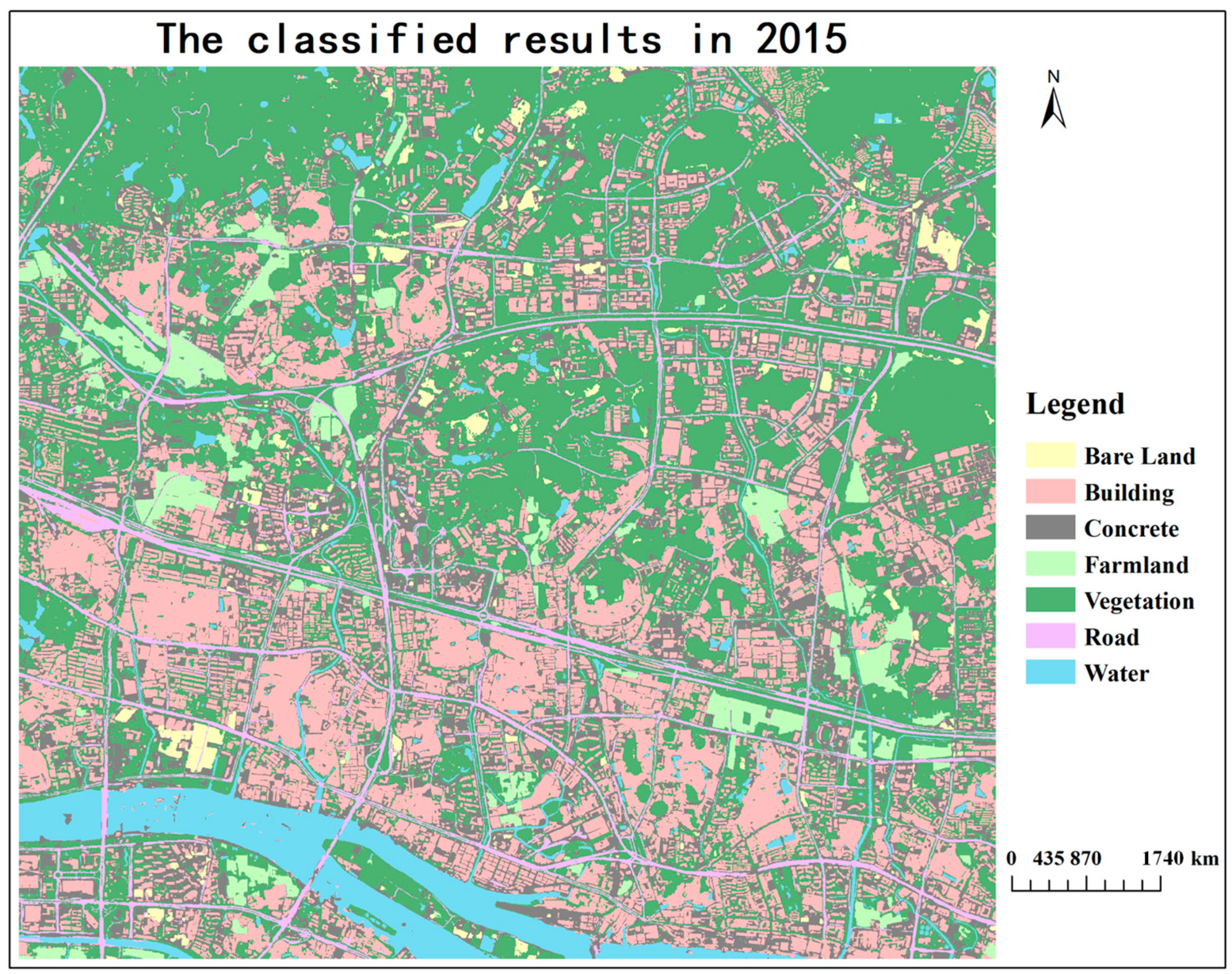
The trained classification model was applied to the classification of high-resolution remote sensing images of the study area in 2015, and the results were shown in Figure 3 We isolated 200 evenly distributed areas of interest as the validation samples, calculated an overall accuracy of 0.875 and a kappa coefficient of 0.8326 according to the confusion matrix of the classification results, and counted the user accuracy (UA) and producer accuracy (PA) of different land use categories, as shown in

Table 3. The user accuracy (UA) and producer accuracy (PA) of different categories in the classified results of the study area in 2015.

Metrics	Bare Land	Building	Concrete	Farmland	Vegetation	Road	Water
PA	0.8333	0.9245	0.9000	0.9359	0.6875	0.7143	0.7143
UA	0.8333	0.9074	0.8182	0.9481	0.8461	0.6897	0.6897

. It can be seen from the table that the classification effect on the concrete and road categories was worse, while other ground object categories achieved a high precision of more than 0.8, which is consistent with the performance of the classification model on the validation dataset. In addition, the best-performing land feature categories on the verification set were farmland and vegetation, respectively, while the confusion matrix calculated using the verification samples showed that the best-performing categories in the UA and PA indicators were vegetation and building, respectively, which proves that vegetation is, indeed, the land use category with the best classification effect. According to the statistical data on the UA and PA indicators, the PA of the building category was not much different from that of farmland, but the UA of the building category was much higher than that of farmland. The reason for this situation may be that the proportion of buildings in the whole research area was much higher than that of farmlands. Therefore, there were a large number of samples with the true value of buildings in the verification samples, and the proportion of misclassification in this category was relatively small.

3.2. The Change Detection Results for 2020

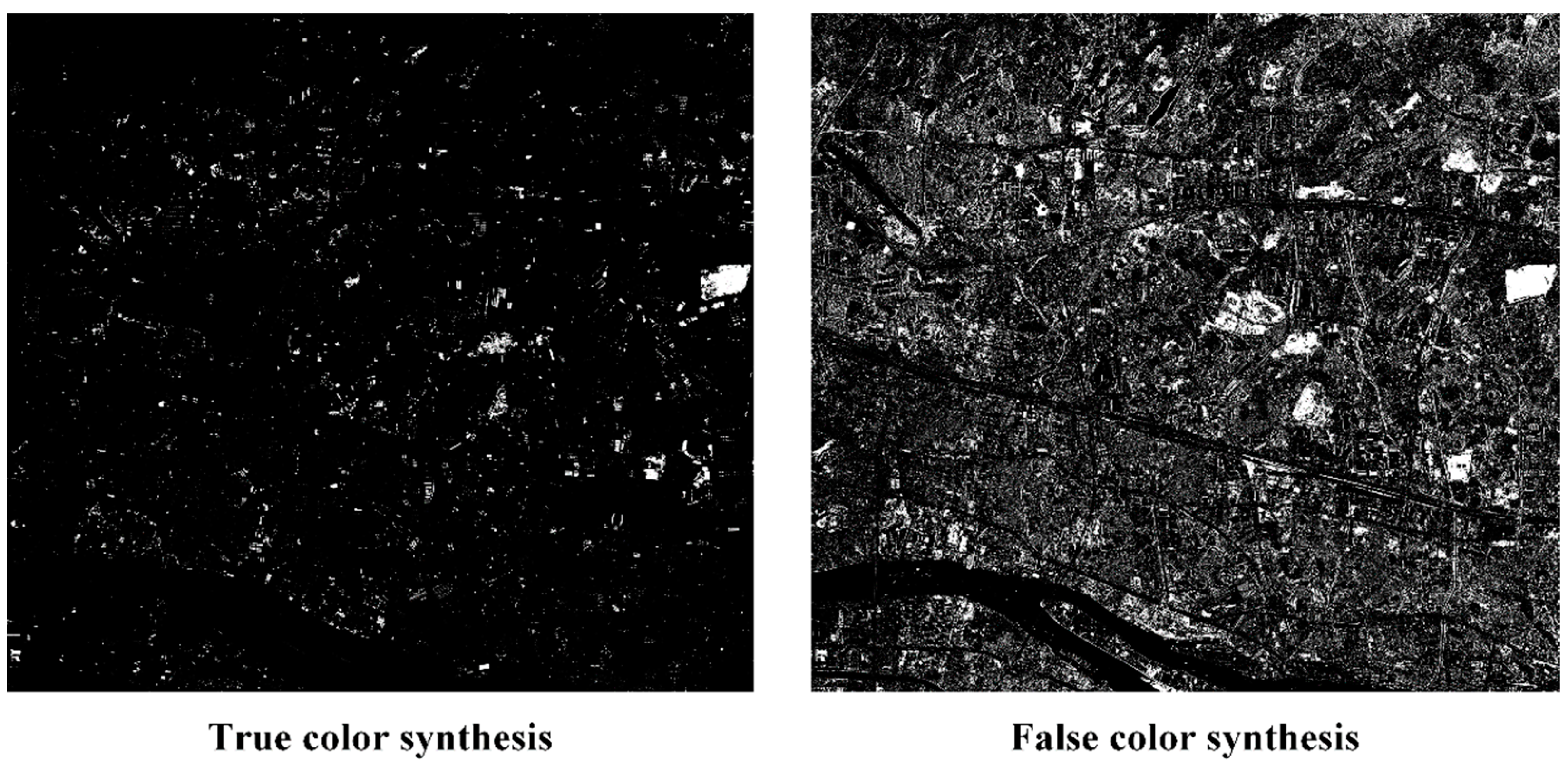
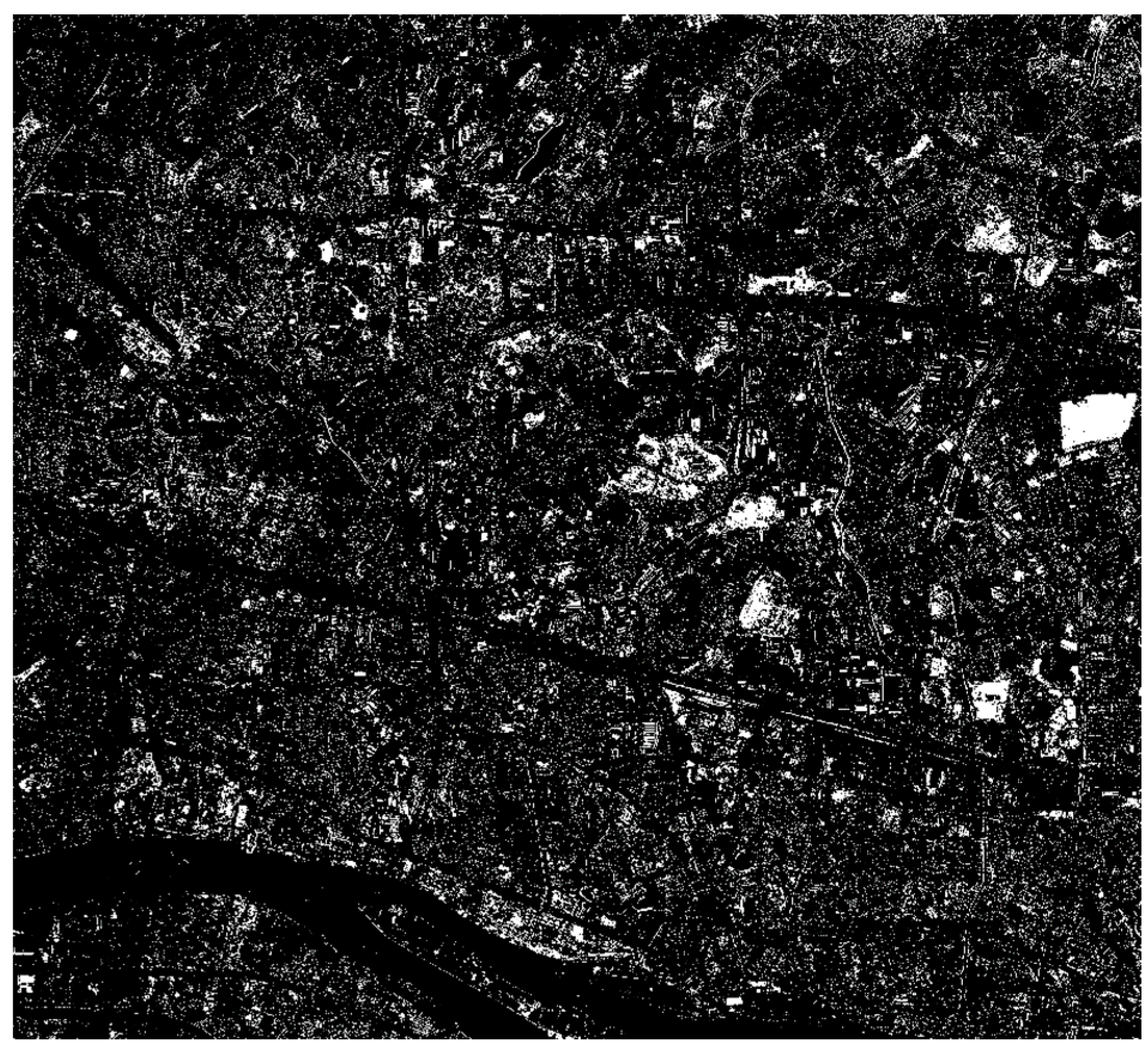
In the preliminary change detection experiments on high-resolution remote sensing images in the research area between 2015 and 2020, which were based on the IR-MAD optimization scheme and on OTSU threshold segmentation, the results of the GF-2 images inputting in IR-MAD using true color and false color synthesis are significantly different, as shown in Figure 4. Most of the changed areas in the figure can be partially detected, and the preliminary change detection results under the false color synthesis on the right show that, in addition to the changed areas, some areas that have not actually changed may also be judged as having partially changed.

Therefore, in the experiment, the difference maps of change detection obtained with true color and false color synthesis were individually processed using Gaussian filtering; then, the two difference maps were superimposed, and the grid average was calculated. Finally, the resulting average difference maps were input for OTSU threshold segmentation, and the preliminary change detection results were finally obtained, as shown in Figure 5.

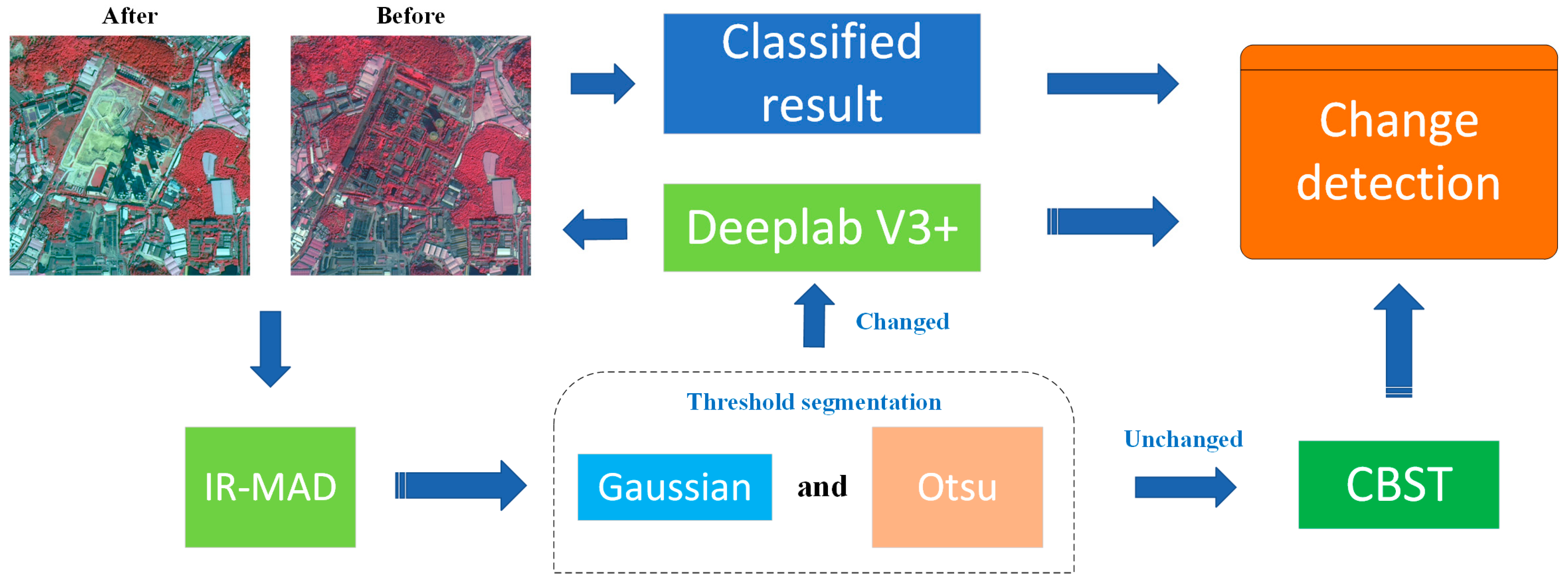
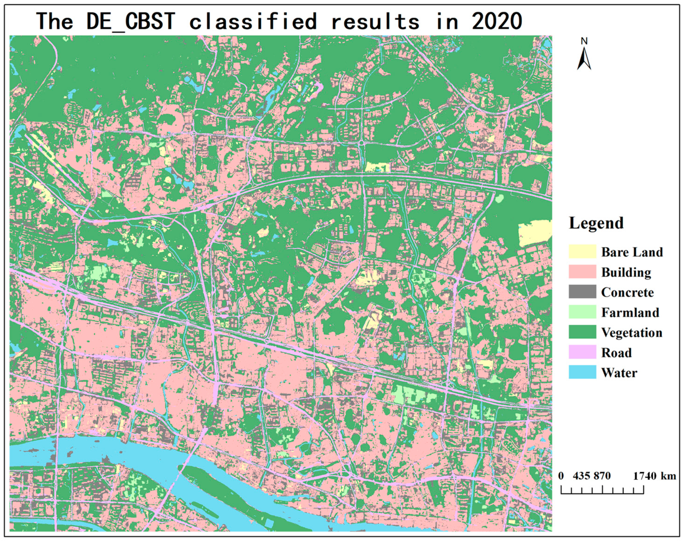
The unchanged region in the IR-MAD preliminary change detection results was used for a CBST region adaptation experiment, and, based on the Deeplab V3+ land use classification model trained on the study area in 2015, we directly migrated to the study area in 2020 through the training sample dataset and validation set of the changed area. Then, the classification results in 2020 of the changed and unchanged regions were fused, and the complete DE_CBST classification results on the GF-2 images of the study area in 2020 were finally obtained (as shown Figure 6). In order to compare the classification accuracy of the DE_CBST experiment and the change detection accuracy relative to the classification results on the study area in 2015, the classification models of CBST region-adaptive experiment training and Deeplab V3+ direct migration were separately applied to the overall GF-2 images’ classification of the study area in 2020. In addition, the U-Net and SegNet models were selected as the comparison models to further compare and verify the accuracy of DE_CBST. In order to maintain the consistency of other parameters in the experiment involving these two classification models, the Deeplab V3+ land use classification model trained on the study area in 2015 was directly transferred to the U-Net and SegNet models for training, and its training sample dataset, validation sample dataset, training iteration number, batch size, and other parameters were consistent with the Deeplab V3+ transfer learning experiment.

In the accuracy evaluation process, 200 evenly distributed areas of interest were selected as the validation samples; the confusion matrix was designed according to the classification results of each experiment in 2020, and the overall accuracy and kappa coefficient were calculated (as shown in

Table 4. Comparison of overall accuracy (OA) and kappa coefficient of the classified results in 2020.

Metrics	U-Net	SegNet	CBST	Deeplab V3+	DE_CBST
OA	0.7500	0.7100	0.7300	0.8100	0.8250
Kappa	0.6710	0.6197	0.6396	0.7501	0.7746

). According to

Table 5. Comparison of the user’s accuracy (UA) and producer’s accuracy (PA) of different classifiers.

Classifiers	Metrics	Bare Land	Building	Road	Concrete	Farmland	Vegetation	Water
U-Net	PA	0.8750	0.7778	0.6250	0.5556	0.3750	0.9437	0.1111
	UA	0.4118	0.8265	0.5263	0.6667	0.7500	0.9178	0.5000
SegNet	PA	0.7500	0.6296	0.6250	0.6667	0.5000	0.8873	0.3333
	UA	0.6000	0.7391	0.4255	0.6667	1.0000	0.8873	0.7500
CBST	PA	0.1000	0.8491	0.5455	0.4375	0.3636	0.9275	0.8750
	UA	0.3333	0.7143	0.5294	0.6364	0.8000	0.8421	0.8750
Deeplab V3+	PA	0.8750	0.7778	0.7813	0.7222	0.5000	0.9296	0.5556
	UA	0.7000	0.8571	0.5814	0.8125	1.0000	0.9167	0.8333
DE_CBST	PA	0.8333	0.8462	0.5946	0.8750	0.8750	0.9104	0.8750
	UA	0.6667	0.8462	0.6667	0.7368	0.8750	0.9242	1.0000

, the DE_CBST classification results achieved the highest overall accuracy and kappa coefficient among all the classification models, while the SegNet classification results were the worst. The classification performance of the other three models was as follows: Deeplab V3+, U-Net, and CBST, in order from best to worst.

In addition, the user accuracy and producer accuracy for each land use category in the 2020 classification results of different models were calculated. According to the statistical data on the PA and UA of different land use categories in the classification results shown in Table 5, it can be seen that the overall DE_CBST classification results have better classification effect than the other models. According to the classification effect on different land use categories, vegetation is the best land use category in all the classification models, and its producer accuracy and user accuracy were both above 0.8. Moreover, the PA of the building category in the SegNet classification model was less than 0.7; the PA and UA of the building category in the other classification models were above 0.7, which proves that the building category in all the classification models experienced a good classification effect. The concrete category did not perform well with respect to the classification effect of all the classification models, which was similar to the classification results on the study area in 2015. In addition, the CBST region adaptation experiment conducted a migration experiment based on samples from the unchanged region, while the bare land category in the changed region showed worse PA and UA scores of less than 0.4, which proves that the CBST model trained using bare land samples from the unchanged region could not identify bare land in the 2020 study area.

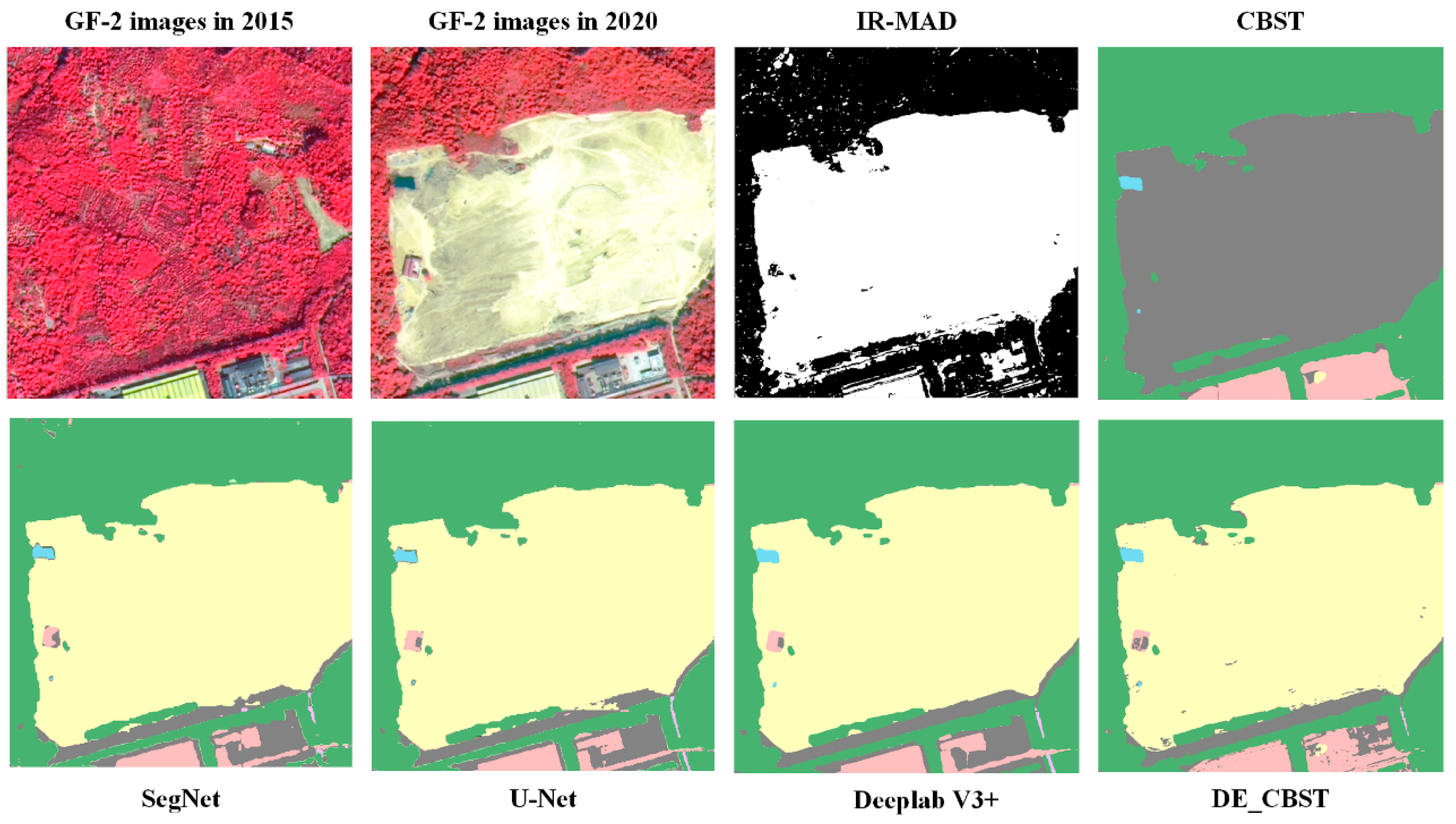
By comparing the classification results of different classifiers for the changed area in 2020 (as shown in Figure 7), it can be seen that, when a large area of vegetation changed into bare land, CBST identified this area as concrete. The three classification models U-Net, SegNet, and Deeplab V3+, which were trained based on a sample dataset of the changing region, could all identify bare land precisely. Therefore, among the classification results of these three classification models, the PA and UA of the bare land category are much higher than those of the CBST model. The classified results of Deeplab V3+ showed the best performance (PA = 0.8750, UA = 0.7). In addition, since the vegetation change had been identified as bare land in the IR-MAD preliminary change detection results, the corresponding changed areas in the Deeplab V3+ classified results were spliced into the classification results of CBST’s invariant areas. Finally, the UA and PA of the DE_CBST classification results were significantly improved compared to the CBST classification results (PA = 0.8333, UA = 0.6667). According to Table 5, since most water regions in the study area experienced little change from 2015 to 2020, the water category could achieve a good performance with PA and UA greater than 0.85 in the CBST classification results. Due to a lack of water samples in the training of the U-Net, SegNet, and Deeplab V3+ classification models, the water classified in the study area using these models showed worse accuracy values in its PA, which was less than 0.6.

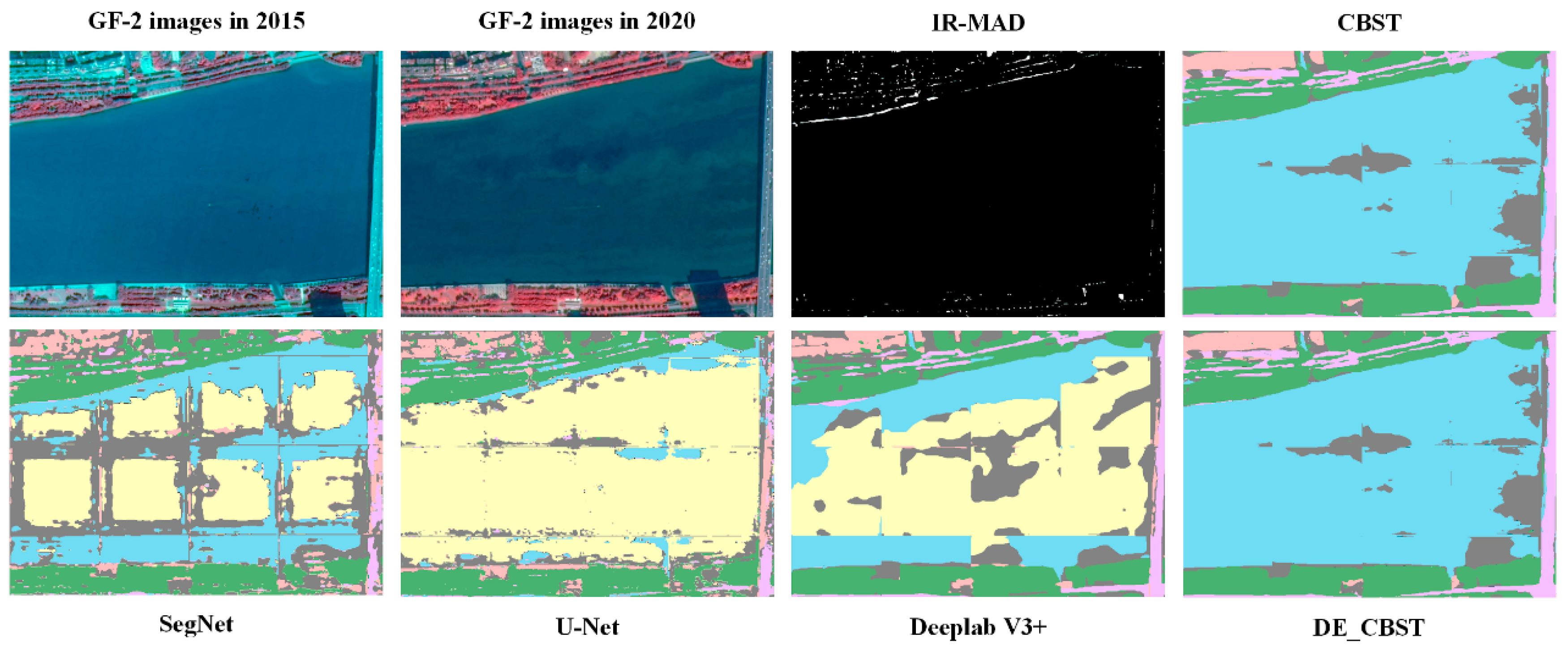
According to the unchanged water region in Figure 8, a large area of water was identified as bare ground and concrete by the three classifiers U-Net, SegNet, and Deeplab V3+, while only a small amount of area was identified as concrete in the classification results of CBST, and most areas could be more accurately identified as water by the CBST model. In addition to the lower PA of the water category, the UA of the bare land and concrete categories in the classified results of the U-Net, SegNet, and Deeplab V3+ models were lower than those of PA. IR-MAD preliminary change detection identified the large area of water shown in Figure 8 as an unchanged area; so, after the classification results of CBST in the unchanged area were superimposed onto the classification results of Deeplab V3+’s changed area, the final water accuracy obtained using DE_CBST significantly improved compared to Deeplab V3+ (PA = 0.8750, UA = 1.0).

The classification results of the five models on the GF-2 images of the 2020 study area were superimposed onto the classification results on the 2015 study area to obtain the change detection results for the 2015–2020 study area, and 200 evenly distributed areas of interest were selected as change detection verification samples. According to the comparison of the change detection accuracy obtained by superposition of the classification results of the five models in

Table 6. Comparison of different classifiers for change detection accuracy in the study area from 2015 to 2020.

Classifiers	Commission	Omission	Precision	Recall	F1	OA
U-Net	0.1964	0.1000	0.8036	0.9000	0.8491	0.8400
SegNet	0.2281	0.1287	0.7719	0.8713	0.8186	0.8050
CBST	0.1800	0.1881	0.8200	0.8119	0.8159	0.8150
Deeplab V3+	0.1667	0.1089	0.8333	0.8911	0.8612	0.8550
DE_CBST	0.1415	0.0990	0.8585	0.9010	0.8792	0.8750

Commission represents the proportion of negative samples predicted to be positive samples to the total negative samples, and omission refers to the proportion of positive samples predicted to be negative samples to the total positive samples.

and the classification results on the research area in 2015, it can be seen that the commission indicator of the DE_CBST change detection results is the lowest, at 0.1415; the omission indicator is the only value lower than 0.1, and the other index values of DE_CBST are also the highest in their category. The F1 index is 0.8792; the overall accuracy is above 0.85, and the kappa coefficient is also greater than 0.75, which proves that the change detection accuracy of DE_CBST is the best among all the models and can be used for further analytical applications. In addition, DE_CBST achieved the maximum accuracy in change detection, resulting in a gain of 2.5% in precision, 1% in recall, and 1.8% in F1 compared to the Deeplab V3+ method. In comparison to the CBST, the respective increases were 3.8%, 8.9%, and 6.3%. Furthermore, the DE_CBST model exhibits lower commission and omission compared to both the Deeplab V3+ and CBST models. Specifically, commission was 2.5% lower than Deeplab V3+’s and 3.9% lower than CBST’s. Similarly, omission was 1% lower than Deeplab V3+’s and 8.9% lower than CBST’s. When compared to the semi-supervised change detection algorithm CDNet + IAug with DE_CBST, it was observed that DE_CBST achieved higher recall and F1 scores when CDNet + IAug marked 20% of the samples on public datasets Levi-CD and WHU-CD [15]. Furthermore, the commission and omission indicators of DE_CBST exhibited superior performances compared to the semi-supervised FDCNN method when evaluated on public datasets WV3 Site1, WV3 Site2, ZY3, and QB, all of which possess similar spatial resolution to GF-2 [14]. Therefore, the change detection results of the DE_CBST model were finally selected as the change detection results for the high-resolution remote sensing images in the research area from 2015 to 2020.

3.3. Land Use Change from 2015 to 2020

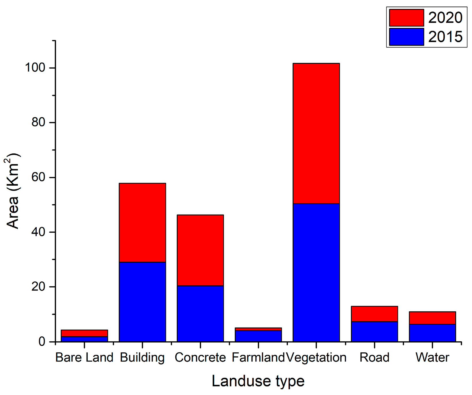
As shown in Figure 9, the largest proportion of the total area of different types of land use in 2015 and 2020 comprised the vegetation, building, and concrete categories. Among these, the total area occupied by vegetation and buildings changed little, and the total area occupied by vegetation was about 50 km². The total area occupied by buildings was about 29 km². The overall area changed in the road and water bodies categories was also less than 1 km², of which the overall area occupied by water bodies was about 6 km² and the overall area occupied by roads about 7 km². In addition, the total area belonging to the concrete category in the study area in 2020 increased by about 3.57 km², compared to the 20.42 km² measured in 2015, while the total area occupied by farmland decreased, from 4.09 km² in 2015 to less than 1 km², with a large percentage of change.

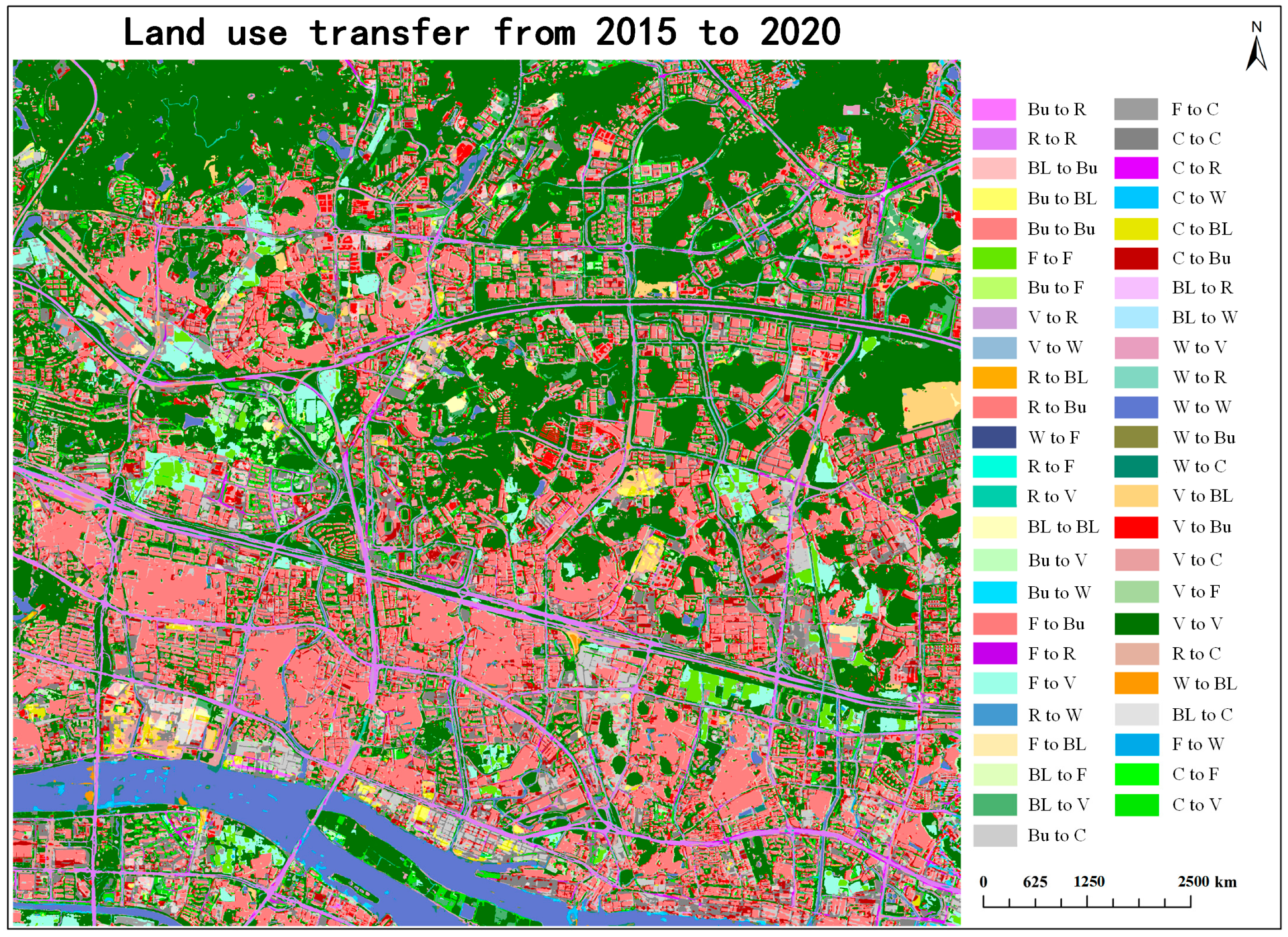
Based on the change detection results on the GF-2 images in the study area from 2015 to 2020, the land use transfer matrix and spatial distribution map of the study area from 2015 to 2020 were prepared, respectively, as shown in

Table 7. Land use transfer matrix in study area from 2015 to 2020.

	2020	Bare Land	Building	Road	Concrete	Farmland	Vegetation	Water	Rate of Change
2015
Bare Land		0.1824	0.3344	0.5955	0.0000	0.6899	0.0387	0.0024	90.10%
Building		0.2526	19.8976	5.6499	0.0038	2.8907	0.2407	0.1300	31.54%
Road		0.3317	4.6186	9.6888	0.0099	4.6229	0.8884	0.2560	52.54%
Concrete		0.1189	0.2422	0.5184	0.8628	2.3044	0.0341	0.0137	78.93%
Farmland		1.0597	3.3925	5.8160	0.0889	38.0015	1.5609	0.5482	24.7%
Vegetation		0.0294	0.2923	1.2104	0.0034	1.7668	3.8714	0.1091	46.84%
Water		0.0584	0.1165	0.5026	0.0018	0.6551	0.0567	4.9735	21.86%

Rate of change represents the proportion of area changed by each land use category to the total area of that category in 2015.

and Figure 10. According to Table 7, although the total area of bare land in 2015 was only 1.84 km² (Figure 9), its change rate reached over 0.9, and bare land was mainly transformed into concrete and vegetation. In addition, the change rate of farmland also reached 0.7893, and about 2.3 km² of farmland was transformed into vegetation, resulting in a sharp decrease in the overall area of farmland. This proved that urban renewal in the study area between 2015 and 2020 resulted in an increase in bare land and a substantial reduction in farmland. In addition, water, vegetation, and building were the three types of land use with the smallest rate of change, among which the low rate of change of water was due to the relatively stable land use structure of water in the study area from 2015 to 2020, while the low rate of change of building and vegetation was due to the large overall area of these two types of land use in 2015, and the proportion of the changed area was relatively small. The actual changed area of the building and vegetation use categories amounted to more than 5 km². In the land use transfer of the building, vegetation, and concrete categories in the study area from 2015 to 2020, the most changes in area involved the interconversion process of these three types of land use. Among them, about 5.65 km² and 2.89 km² of the building area were converted to cement flooring and vegetation, respectively, and about 4.6 km² of the concrete area was converted to building and vegetation areas, respectively. In 2015, except for less than 1 km² of vegetation being converted to water and farmland, the area converted to the other four types of land use was more than 1 km². In addition, about 3.39 km² and 5.82 km² were converted to building and concrete areas, respectively. About 1.06 km² and 1.56 km² were also converted to bare land and road areas, respectively. In general, during the land use transfer in the study area from 2015 to 2020, the overall land use pattern of the water, building, and concrete use categories showed little change, while the increase or decrease in bare land and farmland areas, to different degrees, and the conversion of vegetation to different use types and areas mainly reflected the change in land use’s spatial pattern for the process of urbanization in this region.

3.4. The Relationship between Feature Types and LST

Based on PSC, Landsat 8 OLI data in the study area were obtained for LST retrieval, and the spatial resolution of the LST produced was 30 m. Due to the lack of images caused by cloud cover and other factors, the remote sensing image data from the 18th of October, at the end of autumn, was obtained in 2015, and the average LST recorded was about 31.2 °C, while the remote sensing image data from the 2nd of December, at the end of winter, was obtained in 2020, and the average LST was about 22.4 °C. It can be seen that, even in autumn and winter, the temperature in the downtown area of Guangzhou is over 20 °C. According to the spatial distribution of LST in 2015 and 2020 shown in Figure 11, it can be seen that, in 2015, except for the water in the southwest corner and the large vegetation areas in the north and northeast, almost the entire study area showed an LST greater than 30 °C and that the temperature of part of the grid even exceeded 40 °C. However, the LST in most regions was reduced to about 22 °C, with scattered high-temperature regions above 30 °C, at the end of winter in 2020.

In order to explore the correlation between LST and land use type, we conducted Pearson’s correlation analysis based on the classification results and the corresponding LST data in 2015 and 2020, respectively, and obtained statistical data as shown in

Table 8. The correlation between land use categories and LST in the study area.

Year	Building	CR	FV	Water
2015	0.5099	0.5099	−0.5427	−0.6009
2020	0.3243	0.4650	−0.5168	−0.4782

CR refers to concrete and road, and FV represents farmland and vegetation.

. In comparison to the Pearson correlation coefficients reported by Prem et al. regarding the relationship between NDVI and the daytime LST for various land use categories in India [45], the absolute values of the correlation coefficients presented in Table 8 are greater. These results served as evidence that the correlation between the detected changes in ground features in this study and the LST is more robust, thereby indicating the efficacy of the DE_CBST method. In addition, since the materials comprising road and concrete are close to each other, the road and concrete categories were combined into CR, while vegetation and farmland were combined into FV. In addition, due to insufficient data samples of bare land, the correlation between bare land and LST could not be estimated. It can be seen from the statistical data that artificial surfaces such as building and concrete were positively correlated with the LST, while vegetation, farmland, and water were negatively correlated with the LST, and the correlation between the feature types and the LST was stronger in late autumn (2015), when the LST was higher. However, the surface features negatively correlated with the LST in 2015 and 2020 are more strongly correlated than the artificial surfaces with a positive correlation, which seems at odds with other studies [46]. The reason is that the LST data of the two periods were both acquired in autumn and winter, so vegetation, farmland, and water mainly lead the cooling effect [47].

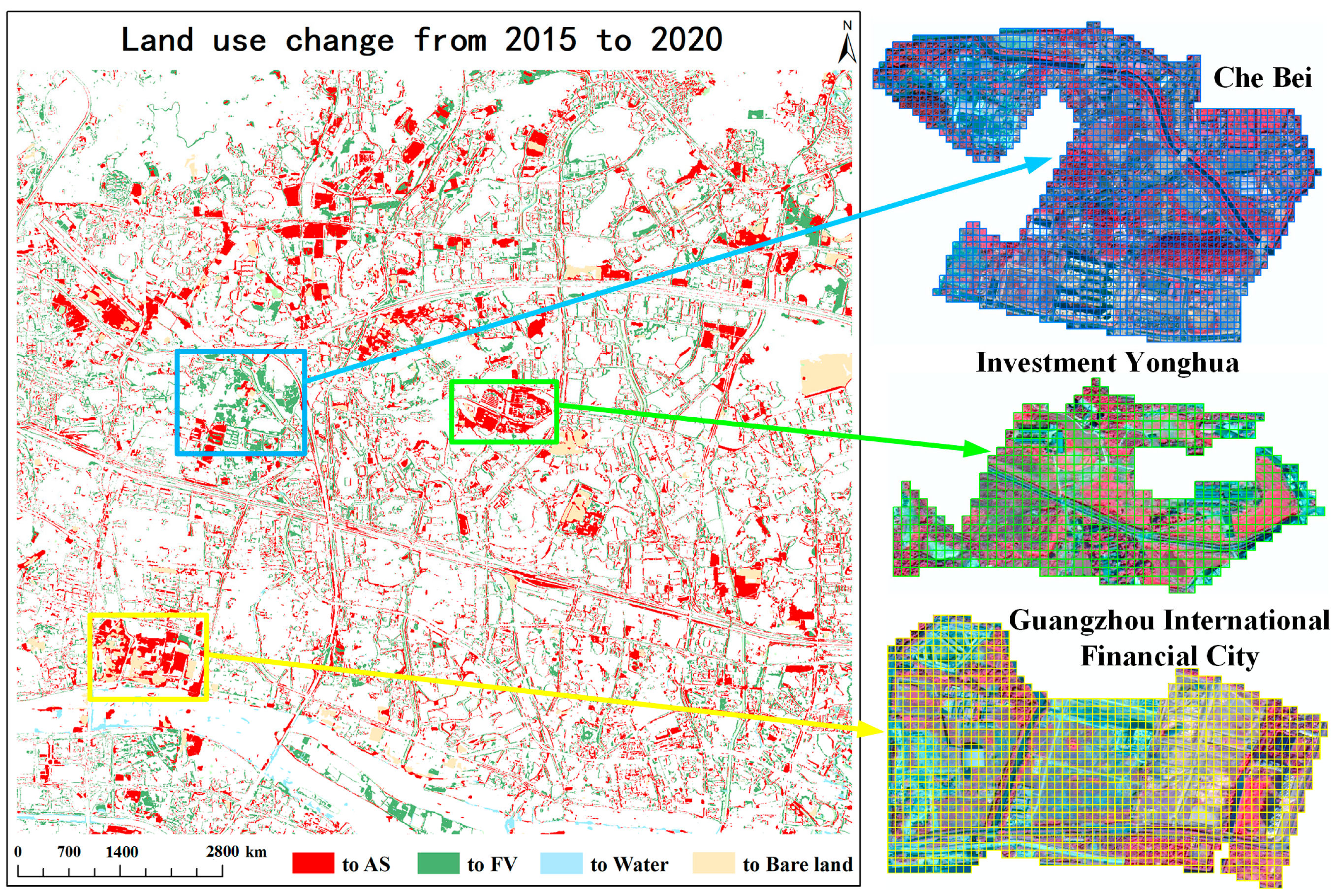
To more specifically target LST and features at a fine-scale, we extracted changed results and produced the 2015–2020 land use change map (Figure 12), in which the building, road, and concrete categories are combined into one category, labeled artificial surfaces (AS). After comprehensive consideration of land use change and LST grid data in the two periods, we selected three regions with more changes within the research area shown in Figure 12 for a GTWR analysis between surface feature categories and LST. The first region selected was Guangzhou International Financial City (GIFC), with an area of about 1.2 km², which was located in the southwest corner of the research area and mainly changed to building and bare land in 2020. The second region was Investment Yonghua (IY), with an area of about 0.6 km², which was located in the center of the research area and mainly changed to buildings in 2020. The last region was Che Bei (CB), with an area of about 1.6 km², which was located on the west side of the center of the study area and mainly changed to vegetation and a few buildings in 2020.

In the GTWR model’s fitting experiment, we first extracted the grid cells with a total of 1430 in GIFC, 678 in IY, and 1937 in CB according to the range of the three selected regions (as shown in Figure 12). Secondly, according to the classification results on the study areas in 2015 and 2020, the area proportions of the building, CR, and FV use categories in each grid were calculated separately. Since the area proportion of water in the three regions was close to zero, the water data were not entered into the GTWR. Then, we took the LST data of each grid in 2015 and 2020 as the dependent variables, and the area proportions of the building, CR, and FV use categories as the independent variables. At the same time, the coordinate factors of latitude and longitude of the grid cells and the time factors were added into the GTWR model for fitting. In order to ensure the consistency of the land surface temperature data and the land use data, a few missing land surface temperature grids in the IY region in 2020 were uniformly removed from the experiment. Finally, the statistical data obtained by fitting the three types of surface features of building, CR, and FV areas into the GTWR model were shown in

Table 9. Results of geographically and temporally weighted regression (GTWR) for the regions.

Region	Bandwidth	Residual Squares	AICc	R2	R2 Adjusted
GIFC	0.1166	2369.83	7713.18	0.9607	0.9607
IY	0.1221	1703.44	4201.36	0.9499	0.9499
CB	0.1098	3172.04	10,387.8	0.9660	0.9660

GIFC refers to Guangzhou International Financial City; IYM refers to Investment Yonghua, and MVA refers to Che Bei.

. The statistical data presented in the table indicate that the R² adjusted values for the three areas surpass 0.9. We performed a comparison of our results with the GWR fitting outcomes for land use/land cover (LULC), topographic elevation, and surface temperature (LST) in Ilorin, Nigeria, as investigated by Njoku et al. from 2003 to 2020, all of which yielded coefficients below 0.9 [48]. It demonstrated that the ground feature results of change detection presented herein exhibited a stronger fitting effect with the LST, which indicated the effectiveness of the DE_CBST model. In addition, since the area of the three regions was IY < G < C, the residual squares value also increased cumulatively with the increase in the number of grids, while the fitting effect (the value of R² adjusted) also increased, simultaneously.

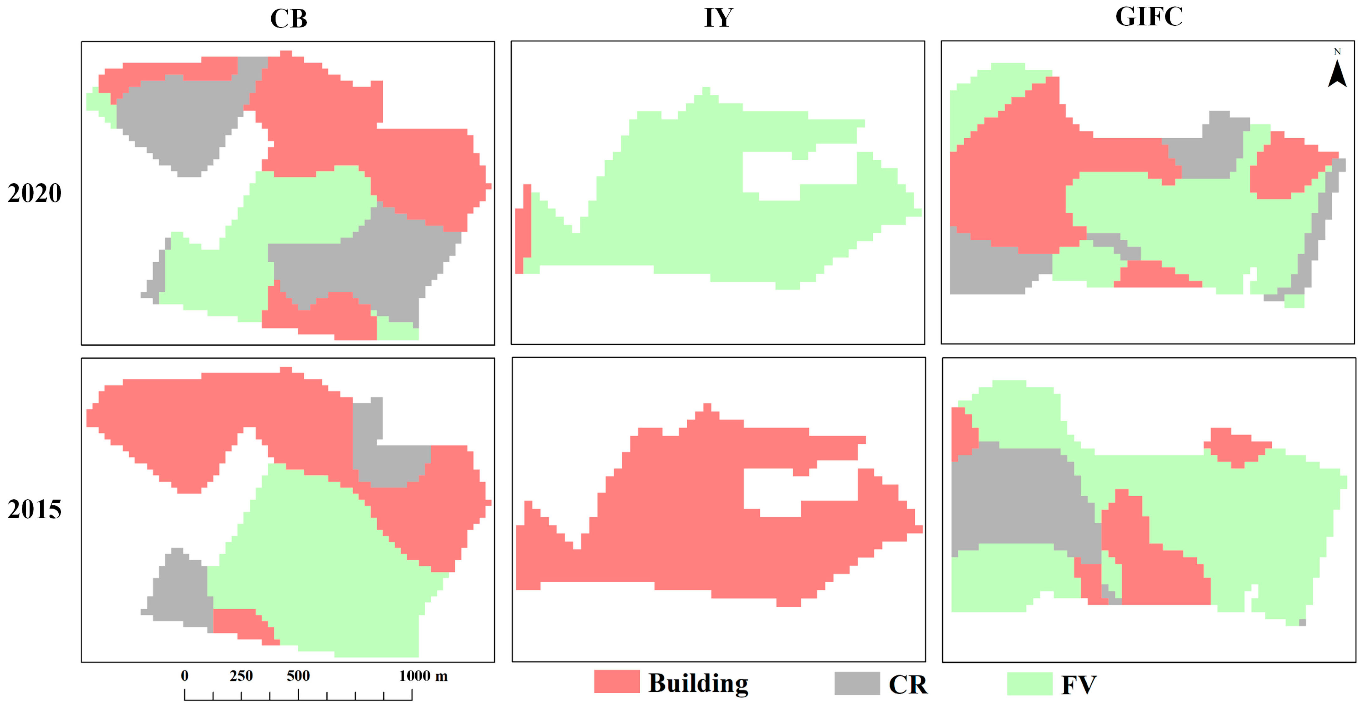
Figure 13 shows the GTWR model’s fitting results for the three regions, where the different colors of the grid cells represent the types of features with the greatest correlation coefficients, which means the types of features with the greatest correlation with LST. According to the change in the correlation coefficient of the GIFC region shown in Figure 13, it can be seen that, even in the case of a low LST in the winter of 2020, the grid cells with a high correlation between building area and LST still occupied more than one-third of the overall area, indicating that the construction of Guangzhou International Financial City buildings promoted the warming effect of the LST. In addition, the higher CR correlation in the west side of the GIFC region in 2015 was due to the fact that part of the plot in 2015 comprised a large area of concrete, while, in 2020, after the change to buildings and, in part, to bare land, the warming effect of the LST was dominated by the building category. In summary, land use change in GIFC substantially increased the building category’s contribution to LST warming in 2020, while it reduced the cooling effect of the FV area on the LST. According to the spatial distribution of the correlation coefficients between the ground features and the LST in the IY region shown in Figure 13, it can be seen that, even though a large area of farmland and vegetation plots in this region changed into multiple residential areas in 2020, the FV category dominated the cooling effect on LST in almost the entire region. However, when farmland and vegetation occupied a large area and only a small part of buildings were built in 2015, the building category dominated the LST warming effect of the entire area. The correlation between LST and ground objects in the IY region seems to be inconsistent with the common view [49] that a large proportion of FV has a strong cooling effect on LST and that a large proportion of buildings has a strong warming effect on LST. There are two reasons for this: On the one hand, the LST of the IY region in the winter of 2020 ranged from 19 °C to 26 °C, so the main FV area with a cooling effect dominated the LST of the whole region, while the LST of 2015 ranged from 28 °C to 39 °C, so the building category, with the strongest LST-warming capacity, dominated the LST of the whole region. On the other hand, IY was located in the easternmost part of the Tianhe District, surrounded by a large area of vegetation. Therefore, in periods of low LST, residential and other buildings within the region can hardly achieve a high warming effect on the LST. According to the spatial distribution of the correlation coefficients between the features and the LST in CB (as shown in Figure 13), it can be seen that, after the factory buildings in the northwest corner of the plot were demolished and turned into CR in 2020, the grid cells of the building category that had led to the LST temperature rising changed into CR. However, due to the completed construction of residential areas and hospitals in the southeastern side of the plot, there was a large proportion of increase in buildings and CR. Despite this, the LST heating grid cells of this part of the region in 2020 were dominated by the CR category rather than the building category. The reason behind this might be that, as the south-eastern block was affected by the Che Bei river across the whole region, from south to north, the warming effect on the LST was weakened by the water, so the correlation between the CR category and the LST seems highest.

4. Conclusions

The study proposed a semi-supervised change detection optimization scheme for multi-temporal high-resolution remote sensing images, which combined IR-MAD, CBST, and Deeplab V3+. The DE_CBST method involved comparing the classification outcomes on the 2020 study area with various models: Deeplab V3+, CBST, U-Net, and SegNet. According to the statistics, DE_CBST achieved the maximum accuracy in change detection, resulting in a gain of 2.5% in the precision indicator and of 1.8% in the F1 score compared to the Deeplab V3+ method. In comparison to the results obtained with the CBST model alone, the respective increases in the DE_CBST model were 3.8% and 6.3%. Furthermore, the DE_CBST model exhibited lower commission and omission scores compared to both the Deeplab V3+ and CBST models. Specifically, commission was 2.5% lower than Deeplab V3+’s and 3.9% lower than CBST’s. Similarly, omission was 1% lower than Deeplab V3+’s and 8.9% lower than CBST’s. Furthermore, the use of DE_CBST significantly enhanced the precision of water identification in unaltered regions, compared to the classification outcomes of Deeplab V3+. Additionally, it notably enhanced the classification performance on bare land in modified regions, compared to the classification outcomes of CBST. In the conducted experiment aimed at investigating the impact of different feature types on LST at a microsurface level, Pearson’s correlation coefficients provided evidence of the positive influence of the building, concrete, and road land use categories on the LST, while they indicated a negative influence of the vegetation, farmland, and water categories on the LST. In addition, the following conclusions can be derived: (1) The GTWR model’s fitting results demonstrated a positive correlation between land use categories and micro-scale LST, indicated a strong association between LST and feature types in the study area during 2010–2020. (2) While, overall, LST changes were generally consistent with local LST changes, variations in LST evolution across different regions suggest some degree of heterogeneity, potentially influenced by the size of the LST region. (3) The correlation between the local LST and the feature types of the associated grid cells did not demonstrate absolute consistency. When conducting an analysis of the local LST, it is crucial to consider the variations in the general LST, the different land use categories in the adjacent vicinity, and the degree of interaction among surface entities.

However, as a result of the constraints imposed by the limited period available for acquiring LST data, this study exclusively utilized LST data from the autumn and winter seasons for the experimental analysis. Future experiments will involve obtaining time series data on land surface temperature (LST) during the spring and summer seasons. Moreover, this study demonstrates a lack of consideration of human variables, like those pertaining to infrastructure development and traffic, in the analysis of the impact of ground characteristics on local LST. Furthermore, there is a deficiency in comprehensive quantitative indicators for human activities. Therefore, it is recommended that future research endeavors focus on addressing these constraints in order to advance our comprehension in this particular field.

References

1. Thangathurai, V.; Thyagharajan, K.K.; Ramya, K. Change Detection using Deep Learning and Machine Learning Techniques for Multispectral Satellite Images. Int. J. Innov. Technol. Explor. Eng. 2019, 9, 90–93. [Google Scholar]
2. Ji, S.; Tian, S.; Zhang, C. Urban Land Cover Classification and Change Detection Using Fully Atrous Convolutional Neural Network. Geomat. Inf. Sci. Wuhan Univ. 2020, 45, 233–241. [Google Scholar]
3. Sefrin, O.; Riese, F.M.; Keller, S. Deep Learning for Land Cover Change Detection. Remote Sens. 2021, 13, 78. [Google Scholar] [CrossRef]
4. Bergamasco, L.; Saha, S.; Bovolo, F.; Bruzzone, L. Unsupervised Change Detection Using ConvolutionalAutoencoder Multi-resolution Features. IEEE Trans. Geosci. Remote Sens. 2022, 60, 1–19. [Google Scholar] [CrossRef]
5. Qin, Y.; Ding, S.; Wang, L.; Wang, Y. Research Progress on Semi-Supervised Clustering. Cogn. Comput. 2019, 11, 599–612. [Google Scholar] [CrossRef]
6. Talaei Khoei, T.; Ould Slimane, H.; Kaabouch, N. Deep learning: Systematic review, models, challenges, and research directions. Neural Comput. Appl. 2023, 35, 23103–23124. [Google Scholar] [CrossRef]
7. Shi, Y.; Ying, X.; Yang, J. Deep Unsupervised Domain Adaptation with Time Series Sensor Data: A Survey. Sensors 2022, 22, 5507. [Google Scholar] [CrossRef]
8. Li, J.; Li, G.; Yu, Y. Adaptive Betweenness Clustering for Semi-Supervised Domain Adaptation. IEEE Trans. Image Process. 2023, 32, 5580–5594. [Google Scholar] [CrossRef]
9. Gu, J.; Qian, X.; Zhang, Q.; Zhang, H.; Wu, F. Unsupervised domain adaptation for COVID-19 classification based on balanced slice Wasserstein distance. Comput. Biol. Med. 2023, 164, 107207. [Google Scholar] [CrossRef]
10. Ganin, Y.; Ustinova, E.; Ajakan, H.; Germain, P.; Larochelle, H.; Laviolette, F.; Marchand, M.; Lempitsky, V. Domain-Adversarial Training of Neural Networks; Csurka, G., Ed.; Domain Adaptation in Computer Vision Applications; Springer International Publishing: Cham, Switzerland, 2017; pp. 189–209. [Google Scholar]
11. Pan, Y.; Yao, T.; Li, Y.; Wang, Y.; Ngo, C.; Mei, T. Transferrable Prototypical Networks for Unsupervised Domain Adaptation. In Proceedings of the 2019 IEEE/CVF Conference on Computer Vision and Pattern Recognition (CVPR), Long Beach, CA, USA, 15–20 June 2019; pp. 2234–2242. [Google Scholar]
12. Li, J.; Meng, L. Review of domain adaptive research. Comput. Eng. 2021, 47, 1–13. [Google Scholar]
13. Ma, L.; Liu, Y.; Zhang, X.; Ye, Y.; Yin, G.; Johnson, B.A. Deep learning in remote sensing applications: A meta-analysis and review. ISPRS J. Photogramm. Remote Sens. 2019, 152, 166–177. [Google Scholar] [CrossRef]
14. Zhang, M.; Shi, W. A Feature Difference Convolutional Neural Network-Based Change Detection Method. IEEE Trans. Geosci. Remote Sens. 2020, 58, 7232–7246. [Google Scholar] [CrossRef]
15. Chen, H.; Li, W.; Shi, Z. Adversarial Instance Augmentation for Building Change Detection in Remote Sensing Images. IEEE Trans. Geosci. Remote Sens. 2022, 60, 1–16. [Google Scholar] [CrossRef]
16. Shen, W.; Peng, Z.; Wang, X.; Wang, H.; Cen, J.; Jiang, D.; Xie, L.; Yang, X.; Tian, Q. A Survey on Label-Efficient Deep Image Segmentation: Bridging the Gap Between Weak Supervision and Dense Prediction. IEEE Trans. Pattern Anal. Mach. Intell. 2023, 45, 9284–9305. [Google Scholar] [CrossRef]
17. Wu, Z.; Yao, L.; Zhuang, M.; Ren, Y. Detecting factors controlling spatial patterns in urban land surface temperatures: A case study of Beijing, Sustain. Cities Soc. 2020, 63, 102454. [Google Scholar] [CrossRef]
18. Wu, P.; Zhong, K.; Wang, L.; Xu, J.; Liang, Y.; Hu, H.; Wang, Y.; Le, J. Influence of underlying surface change caused by urban renewal on landsurface temperatures in Central Guangzhou. Build. Environ. 2022, 215, 108985. [Google Scholar] [CrossRef]
19. Ahmad, J.; Eisma, J.A. Capturing Small-Scale Surface Temperature Variation across Diverse Urban Land Uses with a Small Unmanned Aerial Vehicle. Remote Sens. 2023, 15, 2042. [Google Scholar] [CrossRef]
20. Reiners, P.; Sobrino, J.; Kuenzer, C. Satellite-Derived Land Surface Temperature Dynamics in the Context of Global Change—A Review. Remote Sens. 2023, 15, 1857. [Google Scholar] [CrossRef]
21. Mumtaz, F.; Tao, Y.; de Leeuw, G.; Zhao, L.; Fan, C.; Elnashar, A.; Bashir, B.; Wang, G.; Li, L.; Naeem, S.; et al. Modeling spatio-temporal land transformation and its associated impacts on land surface temperature (LST). Remote Sens. 2020, 12, 2987. [Google Scholar] [CrossRef]
22. Liu, F.; Hou, H.; Murayama, Y. Spatial interconnections of land surface temperatures with land cover/use: A case study of Tokyo. Rem. Sens. 2021, 13, 610. [Google Scholar] [CrossRef]
23. Bala, R.; Prasad, R.; Yadav, V.P. Quantification of urban heat intensity with land use/land cover changes using Landsat satellite data over urban landscapes. Theor. Appl. Climatol. 2021, 145, 1–12. [Google Scholar] [CrossRef]
24. Feyisa, G.L.; Meilby, H.; Jenerette, G.D.; Pauliet, S. Locally optimized separability enhancement indices for urban land cover mapping: Exploring thermal environmental consequences of rapid urbanization in Addis Ababa, Ethiopia. Remote Sens. Environ. 2016, 175, 14–31. [Google Scholar] [CrossRef]
25. Zhou, X.; Chen, H. Impact of urbanization-related land use land cover changes and urban morphology changes on the urban heat island phenomenon. Sci. Total Environ. 2018, 635, 1467–1476. [Google Scholar] [CrossRef]
26. Degefu, M.A.; Argaw, M.; Feyisa, G.L.; Degefa, S. Regional and urban heat island studies in megacities: A systematic analysis of research methodology. Indoor Built Environ. 2022, 31, 1775–1786. [Google Scholar] [CrossRef]
27. Ke, X.; Men, H.; Zhou, T.; Li, Z.; Zhu, F. Variance of the impact of urban green space on the urban heat island effect among different urban functional zones: A case study in Wuhan. Urban For. Urban Green. 2021, 62, 127159. [Google Scholar] [CrossRef]
28. Thanabalan, P.; Vidhya, R.; Kankara, R.S.; Manonmani, R. Time-series analysis of MODIS (LST and NDVI) and TRMM rainfall for drought assessment over India. Appl. Geomat. 2023, 15, 383–405. [Google Scholar] [CrossRef]
29. Zou, Y.; Yu, Z.; Kumar, B.; Wang, J. Domain Adaptation for Semantic Segmentation via Class-Balanced Self-Training. In Proceedings of the European Conference on Computer Vision (ECCV), Munich, Germany, 8–14 September 2018; pp. 289–305. [Google Scholar]
30. Wang, A.; Zhang, M.; Ren, B.; Zhang, Y.; Kafy, A.-A.; Li, J. Ventilation analysis of urban functional zoning based on circuit model in Guangzhou in winter, China. Urban Clim. 2023, 17, 101385. [Google Scholar] [CrossRef]
31. Xing, D. Analysis of China’s High Resolution Satellites and Applications. Satell. Appl. 2015, 03, 44–48. [Google Scholar]
32. Liu, X.W.; Liu, C.Y. An Optional Gauss Filter Image Denoising Method Based on Difference Image Fast Fuzzy Clustering. AMM 2013, 411–414, 1348–1352. [Google Scholar] [CrossRef]
33. Chen, Z. Research on Intelligent Change Detection Technology of High-Resolution Remote Sensing Image; National University of Defense Technology: Changsha, China, 2019. [Google Scholar]
34. Nielsen, A. The Regularized Iteratively Reweighted MAD Method for Change Detection in Multi- and Hyperspectral Data. IEEE Trans. Image Process. A Publ. IEEE Signal Process. Soc. 2007, 16, 463–478. [Google Scholar] [CrossRef]
35. Wu, C. Research on Multi-Layer Information Change Detection in Remote Sensing Image; Wuhan University: Wuhan, China, 2015. [Google Scholar]
36. Chen, L.-C.; Zhu, Y.; Papandreou, G.; Schroff, F.; Adam, H. Encoder-Decoder with Atrous Separable Convolution for Semantic Image Segmentation. arXiv 2018, arXiv:1802.02611. [Google Scholar]
37. Ahmadzadeh, A.; Chen, Y.; Puthucode, K.R.; Ma, R.; Angryk, R.A. TS-MIoU: A Time Series Similarity Metric Without Mapping. In Joint European Conference on Machine Learning and Knowledge Discovery in Databases; Springer Nature: Cham, Switzerland, 2023; pp. 87–102. [Google Scholar] [CrossRef]
38. Lei, L. Research on Time Series Classification and Change Detection Method of Remote Sensing Image Based on Cyclic Neural Network Model. Ph.D. Thesis, Institute of Remote Sensing and Digital Earth, Chinese Academy of Sciences, Beijing, China, 2019. [Google Scholar]
39. Guo, S.; Jin, Q.; Wang, H.; Wang, X.; Wang, Y.; Xiang, S. Learnable gated convolutional neural network for semantic segmentation in remote-sensing images. Remote Sens. 2019, 11, 1922. [Google Scholar] [CrossRef]
40. Jiménez-Muñoz, J.C.; Sobrino, J.A. A generalized single-channel method for retrieving land surface temperature from remote sensing data. J. Geophys. Res. Atmos. 2004, 109, D08112. [Google Scholar] [CrossRef]
41. Sun, D.; Pinker, R.T. Retrieval of surface temperature from the MSG-SEVIRI observations: Part I. Methodology. Int. J. Remote Sens. 2007, 28, 5255–5272. [Google Scholar] [CrossRef]
42. Duan, S.B.; Chen, R. Research progress of land surface temperature remote sensing retrieval from thermal infrared data of Landsat satellite. J. Remote Sens. 2021, 25, 1591–1617. [Google Scholar]
43. Wang, M.; Zhang, Z.; Hu, T.; Liu, X. A practical single-channel algorithm for land surface temperature retrieval: Application to Landsat series data. J. Geophys. Res. Atmos. 2019, 124, 299–316. [Google Scholar] [CrossRef]
44. Huang, B.; Wu, B.; Barry, M. Geographically and temporally weighted regression for modeling spatio-temporal variation in house prices. Int. J. Geogr. Inf. Sci. 2010, 24, 383–401. [Google Scholar] [CrossRef]
45. Pandey, P.C.; Chauhan, A.; Maurya, N.K. Evaluation of earth observation datasets for LST trends over India and its implication in global warming. Ecol. Inform. 2022, 72, 101843. [Google Scholar] [CrossRef]
46. Adeyeri, M.O.E.; Akinsanola, A.A.; Ishola, K.A. Investigating surface urban heat island characteristics over Abuja, Nigeria: Relationship between land surface temperature and multiple vegetation indices. Remote Sens. Appl. Soc. Environ. 2017, 7, 57–68. [Google Scholar] [CrossRef]
47. Khan, M.S.; Ullah, S.; Chen, L. Variations in Surface Urban Heat Island and Urban Cool Island Intensity: A Review Across Major Climate Zones. Chin. Geogr. Sci. 2023, 33, 983–1000. [Google Scholar] [CrossRef]
48. Njoku, E.A.; Tenenbaum, D.E. Tenenbaum. Quantitative assessment of the relationship between land use/land cover (LULC), topographic elevation and land surface temperature (LST) in Ilorin, Nigeria. Remote Sens. Appl. Soc. Environ. 2022, 27, 100780. [Google Scholar]
49. Dissanayake, D. Land Use Change and Its Impacts on Land Surface Temperature in Galle City, Sri Lanka. Climate 2020, 8, 65. [Google Scholar] [CrossRef]
Figure 1. The geographic location of the study area.
Atmosphere 14 01813 g001
Figure 2. The process of the semi-supervised change detection optimization scheme.
Atmosphere 14 01813 g002
Figure 3. The GF-2 classified results of the study area in 2015.
Atmosphere 14 01813 g003
Figure 4. The preliminary change detection results under different image synthesis methods.
Atmosphere 14 01813 g004
Figure 5. The preliminary change detection result using the IR-MAD optimization scheme.
Atmosphere 14 01813 g005
Figure 6. The classified result of DE_CBST in 2020.
Atmosphere 14 01813 g006
Figure 7. Comparison of the classification results of different classifiers in changed areas in 2020.
Atmosphere 14 01813 g007
Figure 8. Comparison of the classification results of different classifiers in unchanged areas in 2020.
Atmosphere 14 01813 g008
Figure 9. The total area of different land use types in the study area in 2015 and 2020.
Atmosphere 14 01813 g009
Figure 10. Land use transfer in the study area from 2015 to 2020. BL refers to bare land; Bu refers to building; C refers to concrete; F refers to farmland; V refers to vegetation; R refers to road, and W refers to water.
Atmosphere 14 01813 g010
Figure 11. Spatial distribution of LST in the study area in 2015 and 2020.
Atmosphere 14 01813 g011
Figure 12. Land use changes from 2015 to 2020. AS refers to artificial surfaces (building, concrete, and road); FV refers to farmland and vegetation.
Atmosphere 14 01813 g012
Figure 13. Spatial distribution of the correlation coefficients between the feature types and the LST in the GTWR results.
Atmosphere 14 01813 g013