Assimilation and Evaluation of the COSMIC–2 and Sounding Data in Tropospheric Atmospheric Refractivity Forecasting across the Yellow Sea through an Ocean–Atmosphere–Wave Coupled Model

Abstract

In this study, a forecasting model was developed based on the COAWST and atmospheric 3D EnVar module to investigate the effects of assimilation of the sounding and COSMIC–2 data on the forecasting of the revised atmospheric refraction. Three groups of 72 h forecasting tests, with assimilation of different data obtained for a period of one month, were constructed over the Yellow Sea. The results revealed that the bias of the revised atmospheric refraction was the lowest if both the sounding and COSMIC–2 data were assimilated. As a result of the assimilation of the hybrid data, the mean bias reduced by 6.09–6.28% within an altitude of 10 km, and the greatest reduction occurred below the altitude of 3000 m. In contrast, the test that assimilated only the sounding data led to an increase in bias at several levels. This increased bias was corrected after the introduction of the COSMIC–2 data, with the mean correction of 1.6 M within the middle and lower troposphere. During the typhoon period, the improvements in the assimilation were more significant than usual. The improved forecasts of the revised atmospheric refraction were mainly due to the moisture changes within the middle and lower troposphere, while the changes in the upper troposphere were influenced by multiple factors.

1. Introduction

Carbon emissions are a contributing factor to shifts in weather patterns and the occurrence of extreme weather events. Therefore, marine weather forecasting is essential to ship navigation, maritime operation, and disaster warning [1,2,3,4]. For several years, due to the lack of observation data, especially the lack of sufficient atmospheric profile data, the accuracy of maritime weather forecasting has been far lower than the accuracy of weather forecasting for lands. Satellite data are one of the few observation data sources for maritime weather forecasting. The advantage of satellite inversion data is that they can provide regional observations, and the inversion data of certain spaceborne sensors can provide three-dimensional changing information of meteorological elements from the top of the atmosphere to the sea surface, thus effectively compensating for the lack of marine observation sites. In the past, a large number of studies based on various meteorological and marine conventional operational satellite data assimilation have made great contributions for the improvement of marine meteorological forecasting [5,6,7]. For instance, Feng et al. assimilated Fengyun-4 satellite data using an ensemble variational data assimilation algorithm with the regional hurricane model HWRF (Hurricane Weather Research and Forecasting model). They found that the trajectory error of the typhoon was reduced by an average of 100 km on the third day of the simulation [8]. Kumar et al. assimilated precipitation data from the Japan Aerospace Exploration Agency satellite using the WRF (Weather Research and Forecasting Model) four-dimensional variational assimilation system. In this study, an improvement of approximately 10% was obtained in temperature forecasting at levels of 600–900 hPa [9]. Xie et al. assimilated satellite data from the AMSU-A (Advanced Microwave Sounding Unit-A) and MHS (Microwave Humidity Sounder) into the RMAPS (Rapid-refresh Multi-scale Analysis and Prediction System) system. They found that the temperature deviation between the levels of 300 and 850 hPa was approximately better by 36.8% as compared to that in the control test that assimilated only the conventional station observations [10].

However, conventional satellite data still needs to be improved in terms of spatiotemporal coverage, resolution, signal-to-noise ratio, etc., in order to provide better assimilation data for numerical predictions [11,12]. In this regard, GNSS (Global Navigation Satellite System) RO (Radio Occultation) technology is one of the remote sensing observation technologies that has developed rapidly in recent years. It is combined with GNSS global navigation satellites by emitting occultations and uses parameters, such as the bending angles, and dry and wet delays, to invert the profile information of atmospheric parameters via tomography techniques. Specifically, when satellite signals pass through the atmosphere, the speed of the signal propagation will change due to atmospheric factors such as air density and temperature, resulting in further changes in the propagation path of the signals [13]. Under the assumptions of local spherical symmetry, ground stations obtain the atmospheric refraction distributions along the occultation-to-ground propagation path through Abel inversion after receiving the occultation radio signals [14]. The advantages of GNSS RO data are their wide coverage and high vertical resolutions, which are good for research related to vertical atmospheric activity [15,16,17].

The COSMIC (Constellation observing System for Meteorology Ionosphere and Climate satellite) is a combined mission of the United States and Chinese Taiwan for the first time to use GPS radio occultation satellites for global weather forecasting. The launch of the COSMIC brings significant improvements in forecasting accuracy over the polar and oceanic regions [18]. At present, COSMIC RO products have been applied for forecasting operations by several agencies like the NCEP (National Centers for Environmental Prediction), ECMWF (European Centre for Medium-Range Weather Forecasts), JMA (Japan Meteorological Agency), and others [19,20,21]. In 2019, the second-generation satellite COSMIC–2 was launched, which is capable of providing more than 5,000 sets of detection profiles daily. The COSMIC–2 has a higher signal-to-noise ratio than the first-generation satellites. Therefore, it enables RO profiles to penetrate deeper into the troposphere to detect atmospheric features in the boundary layers and can provide vertical profiles at a resolution of 0.05 km [22,23]. In addition, COSMIC–2 adopts a novel inversion algorithm, which can provide the profiles of several basic atmospheric parameters, including atmospheric temperature, humidity, water vapor pressure, etc. This feature considerably expands the fields of data application.

Atmospheric refraction refers to the refraction phenomenon that occurs when electromagnetic waves pass through the atmosphere. It is a function of temperature, humidity, air pressure, etc. Atmospheric refraction affects remote sensing image positioning, electromagnetic wave propagation, and ground-space data links and communications [24,25]. Bean and Dutton modified the formula for the calculation of atmospheric refraction so that it is appropriate for ground-based electromagnetic wave transceivers. In this study, they considered the influences of the earth’s curvature on the propagation of ground electromagnetic waves and named the new variable as the revised atmospheric refraction [26]. The formula is described as follows.

$$M=N+0.157\times H$$

(1)

where N is calculated from the expression

$$N=\frac{77.6}{T}(p+4810\frac{e}{T})$$

(2)

Accurate profiles of the revised atmospheric refraction are the data basis for the simulation of ground electromagnetic wave propagation and atmospheric duct diagnosis [27].

According to the formula above, the prediction of revised atmospheric refraction mainly depends on the accuracy of the atmospheric temperature and humidity profiles. However, the forecasting of tropospheric atmospheric humidity in current numerical models still requires further improvements, especially at seas where adequate real-time data cannot be obtained [28]. The launch of COSMIC–2 provides a valuable source of data for mid- and low-latitude marine weather forecasting. It is suitable for all-weather operational assimilation, because its L-band signals are rarely interfered with by clouds and rain. Several previous studies have revealed that the introduction of the assimilation of COSMIC–2 data could improve the accuracy of various weather predictions by certain degrees [29,30]. For example, in terms of prediction of precipitation, Singh et al. used the WRF model and assimilated atmospheric refraction data of COSMIC–2 through a three-dimensional variational assimilation algorithm. The moisture bias in the middle troposphere was correspondingly reduced by 10–20%, and the bias of the temperature and wind in the middle and upper troposphere was reduced by 50–60%. The prediction ability of the model for heavy precipitation was also improved by approximately 20% [31]. Based on the WRF model, Chen et al. assimilated COSMIC–2 occultation data with the 3DEnVar assimilation algorithm and found that the bias of the temperature and wind in the upper atmosphere was reduced. Moreover, the prediction error of the typhoon path and intensity was also reduced [32]. Miller et al. used the HWRF model to simulate six hurricane cases in 2020 and found that assimilating COSMIC–2 data significantly reduced the mean absolute prediction error of the minimum central sea level pressure by 8% to 12% [33].

The Yellow Sea is located in northern China and is a marginal sea where intense human activities occur. The accurate simulation of tropospheric revised atmospheric refraction can provide a significant diagnostic basis for radio meteorological services and research work in this region. In the past, a forecasting system based on the COAWST (Coupled-Ocean-Atmosphere-Wave-Sediment Transport) model was built [34]. Therefore, owing to the high resolution and reliability of COSMIC–2 data, this study intends to further introduce COSMIC–2 RO data into the COAWST forecast system in order to investigate the possible changes in the forecasts of the revised atmospheric refraction over the surrounding areas of the Yellow Sea. In addition, this paper also presents a preliminary discussion on the bias changes from different forecast times.

Section 2 will introduce the data and model used in this study, while Section 3 will introduce the experimental design and configurations of the model. Section 4 will provide a specific analysis of the simulation results. Finally, we will summarize this work and briefly discuss the uncertainty in this study.

2. Data and Model Description

2.1. Observation Data

The observation datasets used for assimilation in this study were radiosonde data and COSMIC–2 RO data obtained over the region around the Yellow Sea in September 2022. The sounding data were obtained from the sounding data website of the University of Wyoming (http://weather.uwyo.edu/upperair/bufrraob.shtml, accessed on 30 November 2023). The elements in the sounding data include altitude, air pressure, temperature, dew point temperature, relative humidity, wind direction, and wind speed. There are 10 sounding stations within the study domain, and their locations are shown in Figure 1a. The sounding data were observed at 00:00 and 12:00 (UTC) daily, of which only the data at 00:00 were used to assimilate the initial values of the model.

COSMIC–2 data were derived from the CDAAC (COSMIC Data Analysis and Archive Center) (https://data.cosmic.ucar.edu/gnss-ro/cosmic2/nrt/level2/, accessed on 30 November 2023). In this study, the wetPf2 near-real-time data set, including pressure, temperature, and humidity, was used for assimilation simulations. The daily dataset contained more than 5000 data files with a vertical resolution of 0.05 km. In this study, we selected the data within three hours around 00:00 every day in September for assimilation. The daily transit trajectories of the COSMIC satellites over the study domain are shown in Figure 1b.

In the following validation process, we used the sounding data as the evaluation references. The radiosonde observations from the Dalian, Qingdao, and Baoshan (in Shanghai) stations were used for evaluations of the forecasting results. Also, the ERA5 (ECMWF Reanalysis v5) reanalysis data were introduced as a cross-comparation with the forecasting results. ERA5 data are the fifth-generation global reanalysis dataset produced by the ECMWF, with a horizontal resolution of 0.25° × 0.25° and 37 vertical layers of atmospheric elements. The ERA5 data were proven to be consistent with station observations across China [35].

2.2. COAWST Model

In this study, the COAWST model was used to construct the simulations for assimilation forecasting. The model was developed by J. C. Warner et al. and included the atmospheric model WRF, the ocean model ROMS (Regional Ocean Model System), and the Ocean Wave Model SWAN (Simulating Waves Nearshore). These component models enabled variable interactions through the model coupling toolkit (MCT) [36]. The COAWST model demonstrates an excellent simulation performance for marine weather changes. For example, Sian et al. studied the impacts of air–sea coupling on the simulations of typhoons over the South China Sea. They found that in comparison to the WRF simulation, the COAWST improved the reliability of the simulation results, and the root mean square error of the 10 m wind speed was reduced by 5.73% [37]. Zheng et al. simulated the super typhoon Megi (2010) via the COAWST model and found that the mean absolute errors in simulating typhoon intensity were decreased by approximately 36% when compared to those in the WRF model [38].

2.3. 3D EnVar Assimilation Module

In this study, the three-dimensional ensemble variational assimilation algorithm (3D EnVar) in the assimilation module of WRF was used to introduce the atmospheric temperature and humidity from the sounding observations and COSMIC–2 into the COAWST simulation, and the initial and boundary fields of the model were constrained accordingly. In 2000, Hamill and Snyder proposed a hybrid assimilation algorithm that linearly combined the static covariance with the background error covariance matrix obtained using the ensemble Kalman filter method when calculating the 3DVAR cost function [39]. Several researchers also made further improvements to this method [40,41,42]. When compared with the performance of the static background error covariance matrix in the 3D Var assimilation, the 3D EnVar algorithm proved to be more adaptable for severe weather simulations. A large number of studies have revealed that this algorithm performs better than the 3D Var in predicting temperature, precipitation, etc. [43].

The assimilation process of 3D EnVar used in this study is listed as follows:

Firstly, a continuous simulation using COAWST was carried out for one month prior to assimilation, and the results were used as samples for calculating the static background error covariance matrix.

Secondly, the sounding and satellite data were processed as an input to the WRFDA system. The temperature and humidity observations from sounding data at 00:00 UTC were collected for assimilation. The COSMIC data needed to be filtered according to the assimilation time and the simulation area. Temperature and humidity profiles near 00:00 UTC every day were filtered and used as observational input for WRFDA along with the soundings.

Subsequently, ten ensemble samples were generated as a first guess for the 3D EnVar by the Random CV scheme. In the scheme, random noises were added to the analysis of control variables, and the mean values of the forecasting ensembles and ensemble perturbations were also calculated. Then, a flow-dependent background error covariance was also derived from the static error covariance and estimated ensemble error covariance. Following this, the files generated above were used as inputs for the minimization process of the 3D EnVar system.

Finally, the analysis field files were updated and then used to replace the initial and boundary field files of WRF.

3. Methodology

3.1. Experimental Design

The study domain in this study was the Yellow Sea with its surrounding areas located in northern China. The Yellow Sea is a flat, semi-enclosed, and shallow sea with an average depth of 44 m. The northwestern side of the Yellow Sea is connected to the Bohai Sea through the Bohai Strait, and the average depth of the Bohai Sea is 18 m. The distribution of the topography and water depth in the region is shown in Figure 1a.

The COAWST model was driven by the atmosphere and ocean forcings to construct forecasting simulation tests for the next 72 h every day. The test period was the whole month of September in 2022. During that period, Typhoon Muifa passed through the coastal areas of the Yellow Sea, which was uncommon in the past few years. Choosing that period for simulation allowed for a more comprehensive evaluation of the performance differences in the forecasting model under extreme and normal weather conditions.

Three sets of simulation tests were designed—t0, t1, and t2. Each test generated the forecasts for the next 72 h every day. The t0 test was the control test without assimilation, and this test initiated the forecasting simulations using the default initial fields. The t1 test used the 3DEnVar module to assimilate the sounding data from 10 stations in the study area (see Figure 1a), and the t2 test assimilated the sounding data as well as the COSMIC–2 data during the simulation period (see Figure 1b for trajectories). By comparing the three tests, we aimed to explore the changes in the forecasting bias after the introduction of the COSMIC–2 data and evaluate the performance of the assimilation of the hybrid data.

3.2. Model Configuration

In this study, the WRF grid numbers were 100 × 100 with a horizontal resolution of 18 km and 39 layers vertically. The ROMS and SWAN grid numbers were 90 × 90 with the same horizontal resolution as that in the WRF model, along with 16 vertical layers for ROMS and one layer for SWAN. Based on the parameterization scheme sensitivity tests carried out in the previous period, the schemes used in the WRF were the GF cumulus scheme [44], the WSM6 cloud microphysical process [45], the RRTM long-wave radiation scheme [46], the Dudhia short-wave radiation scheme [47], the YSU planetary boundary layer scheme [48], the old MM5 surface layer scheme [49], and the MYJ land surface layer scheme [50]. For the ROMS model, the Mellor–Yamada format was used to compute vertical turbulent mixing, and the Flather boundary condition method was used for the barotropic currents [51].

The simulations started on 30 August 2022 00:00 UTC and ended on 1 October 2022 00:00 UTC, and the forecasts during the whole month of September were used for the analysis. The driving data of the WRF were obtained from the GFS (Global Forecast System) (available online at https://ftp.ncep.noaa.gov/data/nccf/com/gfs/prod/, accessed on 30 November 2023), and the driving data of the ROMS were obtained from the RTOFS (Real-Time Ocean Forecast System) (available online at https://ftp.ncep.noaa.gov/data/nccf/com/rtofs/prod/, accessed on 30 November 2023). The driving data of SWAN were obtained from the GFS_wave (Global Forecast System Wave Model) (available online at https://ftp.ncep.noaa.gov/data/nccf/com/rtofs/prod/, accessed on 30 November 2023). In the forecasting simulation process, due to the release time delays, the daily driving data for models actually used the data that were released 24 h in advance.

For the model initialization, ROMS used the default initialization, while SWAN read the restart files obtained before 3 days for a hot restart. Regarding the WRF, the initial data were provided by the 3D EnVar module of the WRFDA. Given the limited number of ensemble members, the background error covariance of the hybrid assimilation in the simulations was used with an ensemble-to-static ratio of 1:1, and the assimilation window for both the sets of assimilation simulations was ±3 h.

4. Result

4.1. Evaluation of the Mean Forecasting Bias at Radiosonde Stations

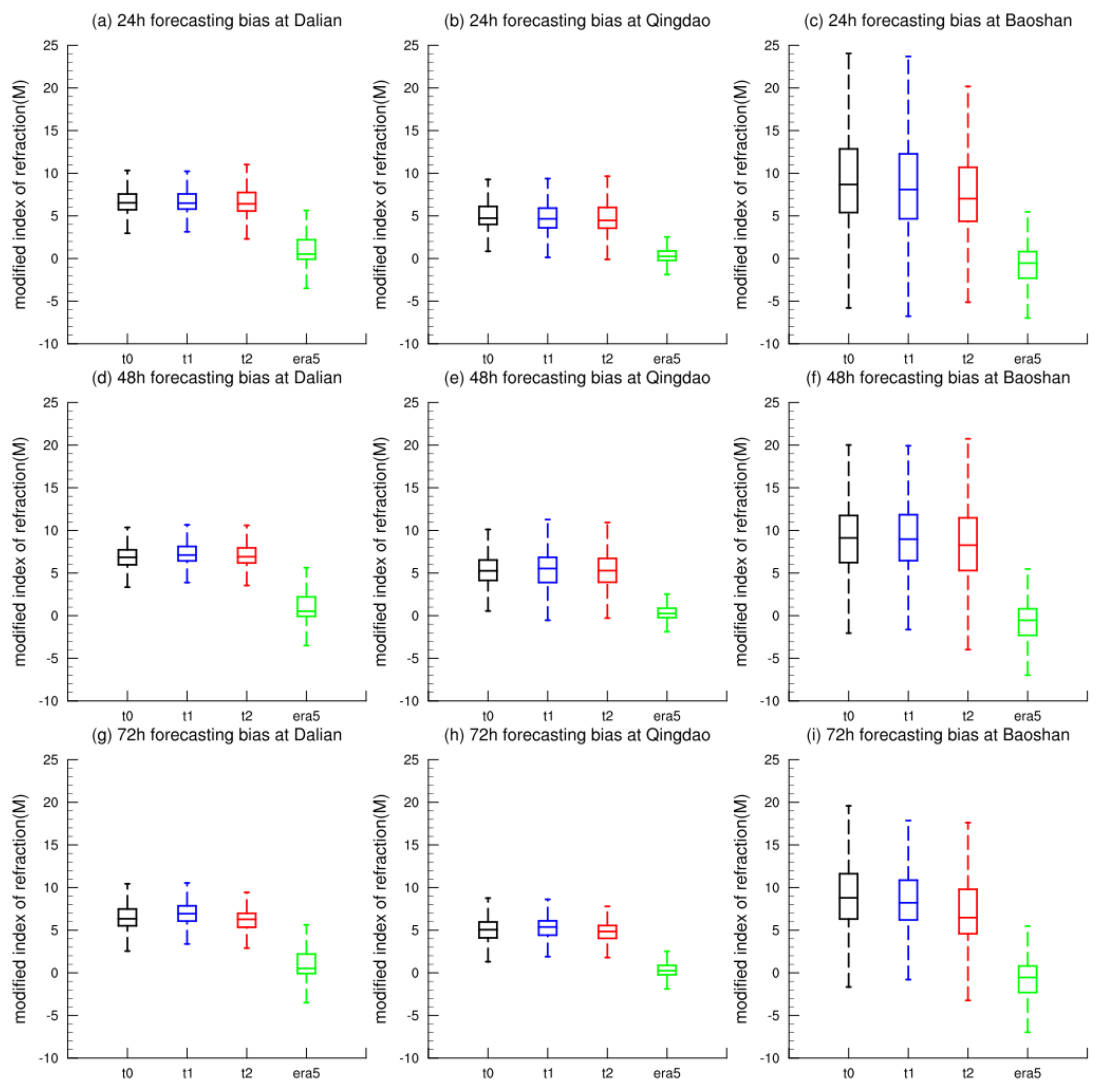
4.1.1. Statistical Distributions of Bias

Based on the time when the forecasts were generated, the three forecasting tests of 72 h ahead (t0, t1, and t2) were further divided into three time series of 24-, 48-, and 72 h forecasts in advance, respectively. The differences among the three series were used to reflect the changes in model performance at different forecasting times. The box plots of the revised atmospheric refraction bias for the three tests (t0, t1, and t2) are given in Figure 2 based on the statistics obtained at the Dalian, Qingdao, and Baoshan radiosonde stations during the entire month of September within the levels from the ground to 10 km.

As shown in Figure 2, all the revised atmospheric refraction biases of the three forecasting tests were maintained within −10 M to +25 M, indicating that the COAWST model with the local parameterization configurations performs effectively in simulating the regional revised atmospheric refraction. In terms of the overall differences among the t0 (black), t1 (blue), and t2 (red) tests, the median bias of the t2 test was the lowest in most cases.

Table 1. The mean bias of revised atmospheric refraction for the t0, t1, and t2 forecasting tests at the three radiosonde stations.

Forecasting Time	Station	Mean Bias
		t0 (M)	t1 (M)	t2 (M)
	Dalian	6.58	6.43	6.41
24 h ahead	Qingdao	4.98	4.77	4.71
	Baoshan	8.73	8.13	7.23
	Dalian	6.89	7.33	6.87
48 h ahead	Qingdao	5.18	5.34	5.22
	Baoshan	8.70	8.82	8.22
	Dalian	6.54	7.00	6.39
72 h ahead	Qingdao	4.96	5.12	4.71
	Baoshan	8.50	7.97	7.03

also lists the mean biases of the three tests, and it can be observed that the mean bias of the t2 test reduced by 6.09–6.28% when compared to those in the t0 and t1 tests. Regarding the varying forecasting times, the bias of the COAWST model did not demonstrate significant increases within the forecasting period of 72 h. When compared with that in the 24 h forecasts, the bias of the 72 h forecasting usually increased by no more than 0.57 M.

The bias distributions in the two assimilation tests (t1 and t2) did not change significantly when compared with those in the control test t0. For the forecasts of 48 and 72 h ahead, the median bias in the t1 test that assimilated only the sounding data were sometimes higher than that in the t0 test. This situation was improved in the t2 test, where the median errors of the forecasts of 24 and 72 h ahead were reduced. However, the median errors of the 48 h forecasts still increased slightly.

In terms of the differences among the three stations, the bias distributions were concentrated at the Dalian and Qingdao stations in the north but diverged more at the Baoshan station with a greater mean bias. This indicates that the model parameterization configurations used in this study are more suitable for the simulation in North China. In addition, the ERA5 reanalysis data demonstrated a high accuracy over the domain. The differences between the ERA5 reanalysis data and the sounding data were significantly smaller than the forecasting bias from the COAWST. Also, the difference distributions between the ERA5 data and the sounding data were basically consistent with the forecasting results and demonstrate the regional differences between the north and south regions.

For the two assimilation tests, the t2 test corrected the possible increase in error caused by the t1 test to a certain extent, with both the median and mean bias values lower than those of the t1 test.

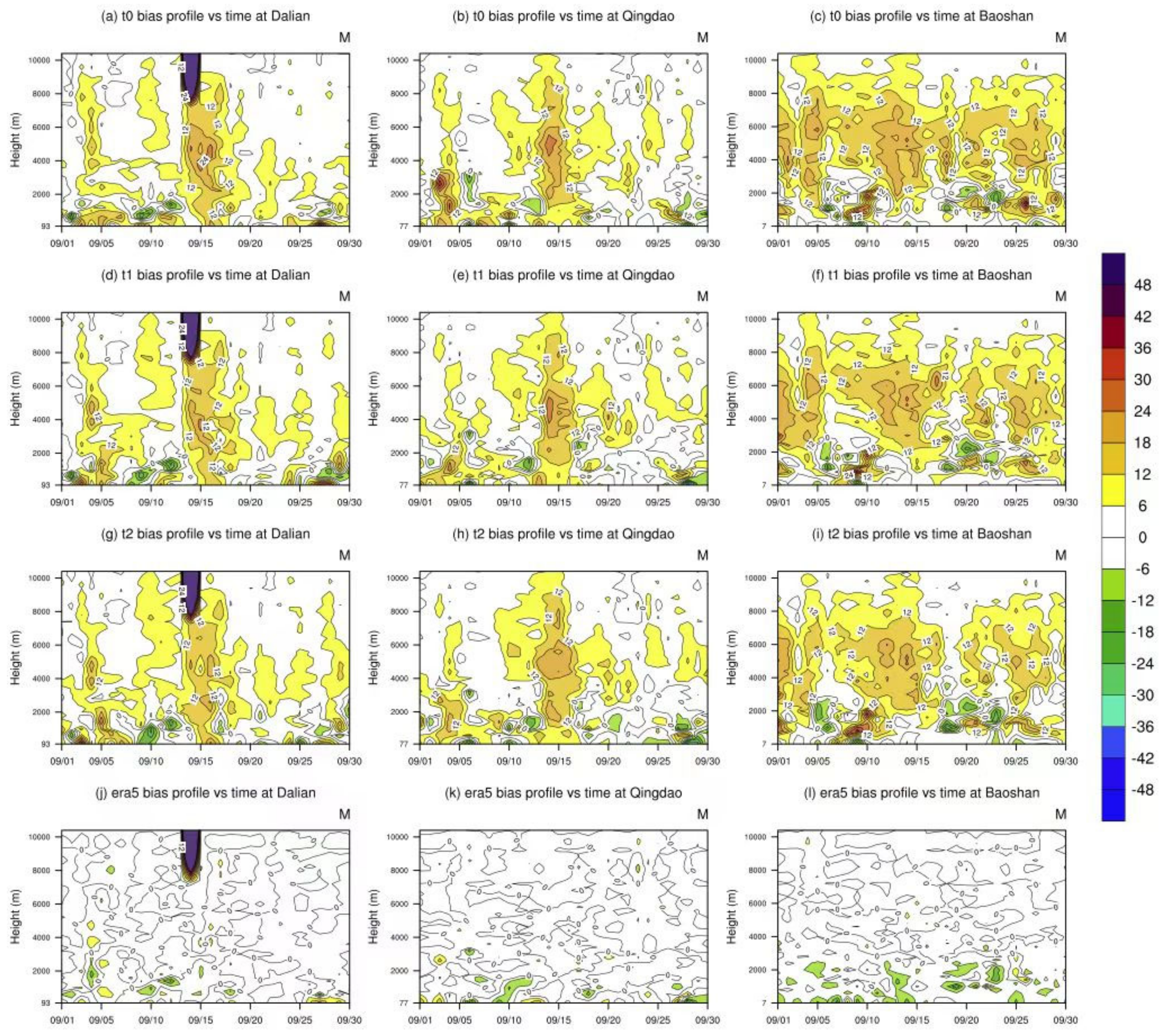
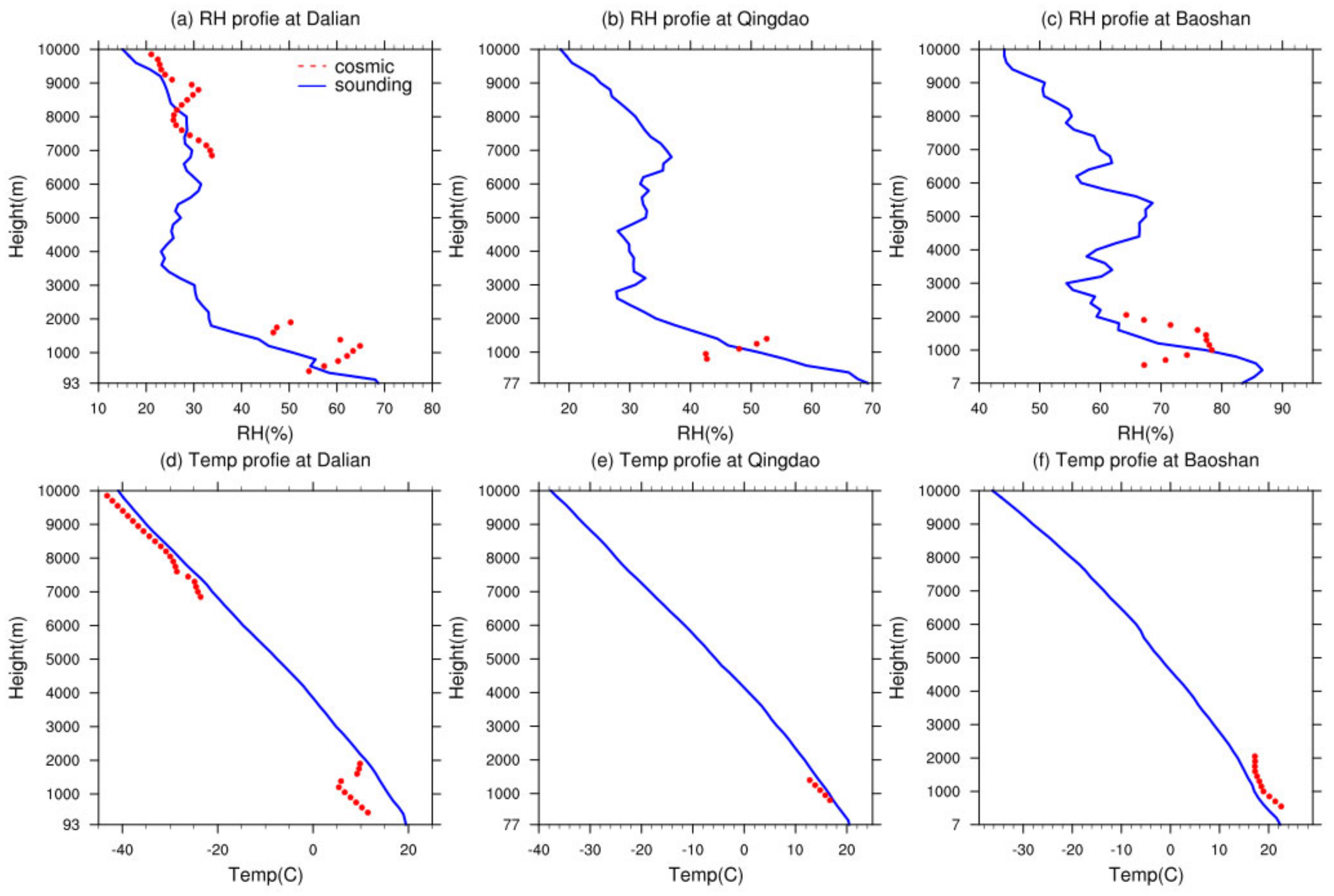
4.1.2. Comparison of the Bias Profiles

In order to investigate the vertical distribution of the revised atmospheric refraction bias, Figure 3 presents the mean bias profiles of the three forecasting tests from the ground level up to an altitude of 10 km. The minimum values of the vertical coordinates correspond to the altitudes of the three stations, respectively.

As shown in Figure 3, the mean revised atmospheric refraction bias within an altitude of 10 km for the three tests was maintained from −6 M to +16 M. In general, forecasting bias does not exhibit uniform trends with the altitude at the three stations. However, all the profiles demonstrate high biases at the levels of 4000–6000 m, indicating that the forecasts still need further improvements in the simulations at the middle troposphere. Regarding the differences among the three tests, the bias profiles of the t2 test were closest to 0 in most cases. The most significant differences between the t2 test and the others were observed at the levels below 3000 m approximately. The differences are probably related to the vertical distributions of the available COSMIC data for assimilation. Statistically, a total of 91 groups of COSMIC data were assimilated at the three stations within the level of 0–3000 m, accounting for 58% of the total data within the altitude of 10,000 m. The assimilation of more observation data in the lower troposphere led to more reductions in the forecasting bias.

For the t1 test, the assimilation of radiosonde data did not reduce the errors observed in the t0 control test at all levels and might have increased the errors in some cases. This drawback was resolved in the t2 test to a certain extent (e.g., the trend observed within the altitude of 3000 m at the Dalian and Qingdao stations). This improvement in the t2 test was roughly positively correlated with the amount of COSMIC data at that altitude level.

Regarding the bias changes due to different forecasting times, the forecasting bias did not exhibit significant increases within 72 h. Nevertheless, due to the high nonlinearity of the atmospheric system, the differences in the 72 h forecasting bias among the three tests were indeed larger than those of the 24 h forecasting bias.

Regarding the regional differences among the three stations, the vertical variability of the bias was lower at the Dalian and Qingdao stations than that at the Baoshan station. It is worth noting that the mean bias at the Dalian station exhibited an obvious increasing trend with heights above the level of 7000 m. This trend is evidently different from those observed in the other two stations. After analyzing the results, it can not be inferred to be the systematic errors, but to be caused by the large differences between the forecasts and the sounding data on certain days.

In addition, the ERA5 data maintained a high accuracy at all altitudes except for the larger differences with the sounding data at levels above 7000 m at Dalian station.

4.2. Temporal Variabilities of Forecasting Bias at Radiosonde Stations

In order to investigate the temporal variability of the error profiles of the assimilation tests, the X–Y schemes of the revised atmospheric refraction profile of the 24 h forecasts with respect to time are illustrated in Figure 4. The vertical coordinate represents the altitude level, and the horizontal coordinate represents the date.

As shown in Figure 4, the revised atmospheric refraction biases of the three forecasting tests were positive for a majority of the time and were roughly concentrated within the levels of 3000–7000 m. The forecast results of the Dalian station on 13–16 September varied considerably from the sounding data, and the bias could be up to more than 200 M. This high bias caused the unusual increase in the bias above the altitude of 7000 m at the Dalian station, which is depicted in Figure 3. The ERA5 data (Figure 4j) also exhibit similar distributions and, therefore, this feature may be related to the quality of the sounding data.

When the Typhoon Muifa passed across the domain on 15–16 September, the forecasts at both Dalian and Qingdao stations showed a larger bias than normal from the ground to 10,000 m, indicating that the forecasts still need to be improved when simulating extreme weather. The t2 test with the hybrid data assimilation could steadily reduce the forecast error of the model during the whole simulation period, with the most obvious reduction at the Qingdao station from 10 to 15 September, and the highest bias reduction could be up to 20 M. This indicates that the introduction of COSMIC–2 data assimilation can, to a certain degree, reduce the negative effects of the typhoon on the forecasting accuracy of the COAWST model. The differences between the ERA5 data and the soundings are significantly lower than the forecasting bias with only an obvious difference occurring within the levels of 0–2 km.

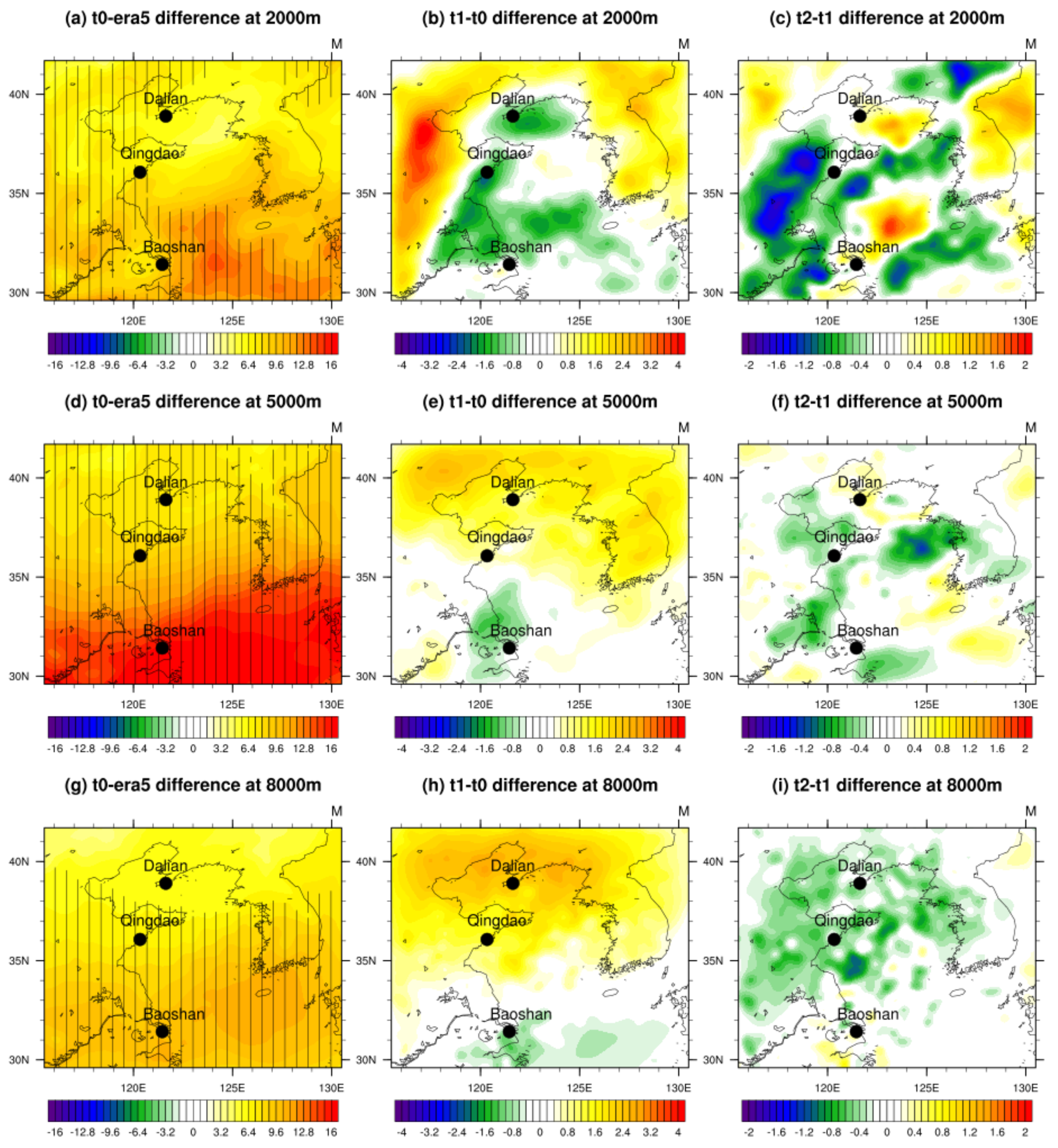
4.3. Regional Analysis of the Changes Due to the COSMIC–2 Assimilation

In view of the abovementioned single-station analysis, the forecasting bias indeed reduced after the introduction of COSMIC–2 data assimilation, and the reduction differed in different regions. In order to further investigate the regional variations of the forecasting bias, the ERA5 data were used as the references in the following analysis to examine the spatial differences among the three tests. Based on the vertical profile distribution of the forecasting bias at single stations described in the previous section, the biases at three specific levels of 2000 m, 5000 m, and 8000 m were selected for the following analysis.

Figure 5 depicts the horizontal distributions of the differences in the 24 h forecasting biases among the three tests at specific levels. The locations of the three sounding stations are marked with black dots. Figure 5a,d,g shows the distributions of the 24 h forecasting bias between the t0 test and the ERA5 data at the levels of 2000 m, 5000 m, and 8000 m. The t0 test demonstrated a significant positive bias at all levels over the domain, and the bias increased from north to south. The forecasting bias at Baoshan station, with the lowest latitude, was significantly larger than that at Qingdao and Dalian stations in the north. At the three different levels, the largest meridional gradients occurred at the height of 5000 m (Figure 5d), which also corresponded to the values of the largest bias, and the bias was up to 15 M.

Figure 5b,e,h depicts the distributions of the difference between the t1 and t0 tests. Due to the assimilation of sounding data, the revised atmospheric refraction simulated by the t1 test was reduced in certain regions, which corrected the positive bias in the t0 test to a certain extent. However, this correction occurred mainly within the lower troposphere above the ocean areas. At other levels or areas, the t1 test further increased the positive bias of the t0 test instead, except for the areas around Baoshan station, where the bias decreased at all levels. These observations of the bias distributions imply that the t1 test does not entirely improve the t0 test in terms of the mean regional bias. According to the statistics of the sounding data of the three stations at each level, the amount of data near the altitude of 2000 m was significantly higher than that at other altitudes. In addition, the amount of sounding data at Baoshan station was more than that at the other two stations near the levels of 5000 m and 8000 m. This indicates that the t1 test can improve the local forecasts over the areas with sufficient sounding observations. However, it may also cause a further increase in bias over the other areas.

To further investigate the regional variations induced by the assimilated COSMIC data, the difference distributions between the t2 and t1 test were observed in Figure 5c,f,i. From this figure, it can be noted that the t2 test effectively corrects the increased bias of the t1 test over most of the areas. This correction occurred at all levels but was most evident near the level of 2000 m, with a regional average correction of up to 1.6 M. The correction at the middle troposphere, i.e., the level of 5000 m, was relatively weakest at the three specific levels.

Since the revised atmospheric refraction is a diagnostic variable from the model outputs, the distributions of the differences in the humidity and temperature bias for the three tests were further examined. Figure 6 shows the distributions of the 24 h forecasting bias of the relative humidity compared with the ERA5 data at each level. As shown by the bias distributions between t0 and ERA5 in Figure 6a,d,g, a lower forecasted humidity was detected by the t0 test in the lower and middle troposphere. The maximum bias occurred near the level of 8000 m, which was up to 15% at most. The differences shaded by strips passed the significance test at a 95% confidence level. After adding the assimilation of the sounding data, as shown in Figure 6b,e,h, a drier atmosphere was simulated in the t1 test when compared to that in the t0 test over most of the region, and there was a significant decrease in the relative humidity near all the three radiosonde stations. The distributions of the difference in humidity between the t1 and t0 tests seem rather similar to the distributions of the difference in the revised atmospheric refraction in Figure 5. Thus, the spatial correlation coefficients between the differences in the revised atmospheric refraction and the differences in relative humidity at specific heights were examined. The coefficients were 0.92 and 0.79 at the levels of 2000 m and 5000 m, respectively, and at the level of 8000 m, the coefficient was 0.30. This indicates that the correlation between the change in the revised atmospheric refraction and the change in the relative humidity decreases with the lifting altitude. In other words, in the lower troposphere, the change in humidity is probably one of the important factors dominating the changes in the revised atmospheric refraction, while this relationship gradually weakens as the altitude increases and the relationship turns out to be inaccurate in the upper troposphere at a low humidity.

The t2 test, with the introduction of the assimilation of COSMIC data, corrected the humidity bias of the t1 test. As shown in Figure 6c,f,i, the difference between t2 and t1 was more or less complementary to the difference between t1 and t0 over many regions. In addition, the spatial correlation coefficients between the humidity bias in Figure 6c,f,i and the revised atmospheric refraction bias in Figure 5c,f,i reached 0.90, 0.71, and 0.23. The correlation also weakened with the increasing altitude.

Similar to Figure 6, Figure 7 also provides the distribution of temperature differences. All temperature differences in the figure did not pass the significance test at a 95% confidence level. Figure 7a,d,g shows the distributions of the temperature bias between the t0 test and ERA5 at three specific levels. A regional cold bias was detected at the levels of 2000 m and 5000 m, and this cold bias shifted to a weak warm bias at the level of 8000 m. As shown in Figure 7b,e,h, the t1 test presents warm differences in most regions at all levels, which can effectively correct the cold bias of the t0 test below 5000 m. In some southern regions of the domain, including the Baoshan station, the t1 test corrects the warm bias of the t0 test, but to a weak degree. Interestingly, with the increasing altitude, the distributions of such dipole-like differences between the north and south in Figure 7b,e,h gradually tend to be similar to the distributions of the differences in the revised atmospheric refraction in Figure 5b,e,h. Their spatial correlation coefficients were −0.08, 0.16, and 0.37, respectively. Considering the humidity differences in the lower and middle troposphere, the moisture factors are likely to dominate the change in the revised atmospheric refraction in the lower and middle troposphere with a higher humidity. On the other hand, the effects of the humidity on the revised atmospheric refraction gradually decrease in the drier upper troposphere, and the roles of the temperature factors become more and more important. Certainly, according to Equation (2), the revised atmospheric refraction is also related to the changes in air pressure. The linear relationship between the pressure change and the changes in the revised atmospheric refraction at each level was examined, and we found that their linear correlation is rather low (figure not shown). Therefore, we can confirm that the changes in the revised atmospheric refraction in the assimilation tests basically arise from the humidity changes in the lower and middle troposphere, instead of the combined changes in multiple factors (including humidity and temperature) in the upper troposphere. For the t1 test with the single source of assimilated data, this effecting relationship is shown quite clearly. However, with the addition of the data from the other sources, the highly nonlinear atmosphere system weakens this relationship, making the system more chaotic.

As shown in Figure 7c,f,i, at the levels of 2000 m and 5000 m, the t2 test weakens the effects of the temperature improvement in the t1 test. However, the bias of the t2 test is still lower than that of the t0 test in value. The distributions in Figure 7i at the level of 8000 m are basically opposite to that of Figure 7h, but the changes in the t2 test are rather tiny. As for the spatial correlation coefficients of Figure 7c,f,i with the corresponding subplots in Figure 5, they are −0.29, 0.09, and 0.18, respectively, and do not demonstrate correlations as high as those observed in the t1 test.

Based on the differences in temperature and humidity among the tests, a further examination was addressed to investigate the causes of these changes. In this study, the 3D EnVar algorithm assimilated only the initial conditions of forecasts and provided no constraints in the course of forecasting simulations. Thus, the differences among the t0, t1, and t2 test stemmed from the observation data assimilated at 00:00 UTC every day, when the forecasts started.

Figure 8 depicts the profiles of humidity and temperature assimilated in the t1 and t2 tests at three sounding stations. Due to the variable satellite trajectory, the COSMIC–2 data at the three station locations cannot cover all altitude levels. Therefore, they are presented in a scattered form.

As shown in Figure 8a–c, the COSMIC data at the locations of the Qingdao and Baoshan stations are concentrated below 2000 m in altitude. The COSMIC data at the Qingdao station are limited and do not exhibit significant differences from the sounding data. In contrast, the COSMIC data at the Baoshan station indicate lower humidity, by over 10%, compared to the sounding data below 1000 m, while its humidity data are slightly higher between 1000 m and 2000 m. The COSMIC data at the Dalian station provide available data for assimilation processes both above 7000 m and below 2000 m in altitude. At most altitudes, the COSMIC humidity data are higher than the sounding data. When these higher-humidity data were assimilated into the modeling system together with the sounding data after blending, they might have led to an initial field in the forecasting model with higher humidity in that region.

Figure 8d–f depict the temperature profiles used for assimilation at three station locations. At the Dalian station, the COSMIC temperature data generally appear lower than the soundings. Specifically, below 2000 m in altitude, some COSMIC temperature data even deviate by more than 10 degrees Celsius from the soundings, which is inconsistent with Dalian’s September climate. This phenomenon indicates that the COSMIC satellites still exhibit certain biases in retrieving temperature and humidity at near-surface heights. As for the temperature observations at the Qingdao and Baoshan stations, the COSMIC data tend to be lower at Qingdao and higher at Baoshan, but the overall differences from the sounding data are not significant.

The discrepancies between sounding data and COSMIC satellite data further led to differences in the initial fields of simulations for the t1 and t2 tests. Figure 9 and Figure 10 illustrate the regional changes in humidity and temperature initial fields after updates by the assimilation system. Similar to Figure 6, Figure 9 depicts the differences in humidity initial fields among the t0, t1, and t2 tests. For reference, the ERA5 reanalysis data at 00:00 each day also participate in the comparison.

As shown in Figure 9a,d,g, the initial humidity field of t0 test exhibits the greatest difference from ERA5 data at a height of 8000 m, with a regional average error reaching −10.8%. The humidity differences in only a few regions passed the significance test at a 95% confidence level. Meanwhile, the average differences at 2000 m and 5000 m heights are maintained within ±2%. Compared to Figure 6, it is evident that the differences between the model’s initial fields and ERA5 data at 00:00 are significantly larger than the average differences during the simulation period. After assimilation of sounding data in experiment t1, the initial humidity at all height levels decreased, with the most pronounced decrease occurring in the northern part of the domain. This change in initial conditions gradually diminished as the simulation time progressed. After 12~16 h, the distribution of humidity differences between the t1 and t0 tests no longer exhibited obvious regional characteristics, but instead displayed a more chaotic pattern of differences. In fact, the decrease in humidity in the central and northern part of domain increased the forecasting bias of the t1 test; however, due to the positive correlation between the atmospheric refraction and humidity changes, this dry bias reduced the higher atmospheric refractivity bias in the t0 test (see Figure 5). When the t2 test introduced the COSMIC data into assimilation, as shown in Figure 9c,f,i, the dry bias in the t1 test was corrected, but overall, it still remained relatively drier than the t0 test.

Similar to Figure 9, Figure 10 also illustrates the differences in the initial temperature field. As shown in Figure 10b,e,h, more pronounced warm difference in north and cool difference in south, compared to Figure 7, was detected in the t1 test. The warm differences in the northern part of domain even pass the significance test at a 95% confidence level. This indicates that the t1 test not only amplifies the north–south humidity difference at the beginning of the simulation but also weakens the north–south temperature gradient. Regarding the changes in revised atmospheric refraction, the northern and western warming caused by the t1 test corresponds closely to the increased atmospheric refraction bias in these regions. As for the t2 test, which conducted hybrid data assimilation, it unsurprisingly partially compensated for the north–south temperature distribution in the initial conditions of t1 test.

In addition, along with the observed warm differences in the northern region of the t1 test’s initial conditions, there were also associated high-pressure differences in the north (figure not shown). To further investigate the variations in regional water vapor transport processes caused by the initial conditions, Figure 11 presents the spatial distributions of average differences in water vapor flux during the simulation period. As shown in Figure 11b,e,h, the t1 test further enhanced the north–south difference in water vapor flux across the Yellow Sea area compared to the t0 test, thereby maintaining the initial dry bias in the northern region (see Figure 9b,e). Consequently, at altitudes of 2000 m and 5000 m, the atmospheric refraction bias was induced to decrease by the reduced humidity in the regions around the Yellow Sea. At an altitude of 8000 m, the water vapor flux difference in the t1 test shifted to a westward flux difference, weakening the westerly jet stream in the upper troposphere. Since the upper troposphere has lower humidity, the water vapor flux difference is primarily attributable to the differences in wind speed. The stronger westward flux differences in the upper troposphere accelerated the decay of the initial condition’s impacts. As for the t2 test in Figure 11c,f,i, the change in water vapor flux was more pronounced at the 2000 m altitude, while the variation at other altitudes was minimal. In the northern part of the domain, the t2 test induced a cyclonic water vapor flux change, enhancing the moisture flux from the northwest direction in Figure 11c, weakening the anticyclonic characteristics observed in the t1 test in the northern region. Consequently, it became challenging to sustain the dry bias at the regional center observed in the t1 test (Figure 6b), ultimately affecting the distribution of revised atmospheric refraction.

5. Discussion and Conclusions

It should be noted that the simulation results of this study have some limitations and uncertainties.

After assimilating the sounding data and COSMIC–2 RO data, significant regional inhomogeneity in the revised atmospheric refraction forecasting existed, with improvements not realized across all regions and altitudes. We calculated the ratio of grid points showing improved forecasting accuracy in the t1 and t2 tests compared to the t0 test. For the t1 test, the improvement ratios at altitudes of 2000 m, 5000 m, and 8000 m were 70.3%, 30.6%, and 46.4%, respectively. After the introduction of COSMIC data, these ratios increased to 79.1%, 30.5%, and 50.9% at the same altitudes. The improvement was particularly pronounced at 2000 m altitude.

As for the bias statistics of the three radiosonde stations shown in Table 1, the t2 test exhibited the lowest average bias within the 0–10,000 m altitude. However, this does not imply that t2 test effectively reduced the bias of the t0 and t1 tests at all radiosonde stations. Therefore, we additionally selected three radiosonde stations (Zhangqiu, Anqing, and Hangzhou) and evaluated the biases of the 24 h revised atmospheric refraction forecasts at these stations. The locations of these stations are shown in Figure 1a. Based on the statistics, the average bias for the t0 test at these three stations were 4.61 M, 7.68 M, and 10.48 M; for t1 they were 4.93 M, 7.35 M, and 9.84 M; and for t2 they were 4.52 M, 7.17 M, and 9.86 M. The t2 test showed the lowest bias at Zhangqiu and Anqing stations, but its bias at Hangzhou station was slightly higher than that of the t1 test. In general, the hybrid data assimilation in the t2 test effectively improved forecasting accuracy in most stations.

Certainly, the forecasting improvements mentioned above are limited to the simulation period, i.e., in September 2022. To enhance the credibility of our conclusions, we additionally conducted forecasting tests for three time periods: 11–15 March, 11–15 June, and 11–15 December, all in 2022. Using the same model configuration, we performed 5-day forecasting simulations.

Table 2. The mean bias of 24 h forecasted revised atmospheric refraction for the t0, t1, and t2 tests during other simulation periods.

Forecasting Period	Station	Mean Bias
		t0 (M)	t1 (M)	t2 (M)
	Dalian	3.07	3.50	3.24
11–15 March	Qingdao	1.79	1.75	1.68
	Baoshan	5.12	5.51	4.77
	Dalian	6.81	6.74	6.64
11–15 June	Qingdao	5.73	5.66	5.29
	Baoshan	2.34	3.47	2.43
	Dalian	3.54	3.62	3.64
11–15 December	Qingdao	3.57	3.48	3.37
	Baoshan	5.49	4.98	4.87

presents the 24 h forecasting biases of revised atmospheric refraction for t0, t1, and t2 tests during these three time periods. The results from these simulation periods are generally consistent with the conclusions based on September in this study. Compared to the t0 test, the t1 test improved about half of the cases. Considering the nonlinearity of the atmospheric system, it should be noted that the t2 test did not uniformly improve forecasting accuracy across all cases. However, it did exhibit the lowest bias in most cases. The results in Table 2 demonstrate that the hybrid data assimilation approach using the sounding and COSMIC data can maintain a good performance across different seasons of the simulation period.

Despite the uncertainties discussed above, there are some aspects which need to be further improved in the future. Firstly, in terms of the model configuration, this study used ten ensemble members to construct the ensemble 3D variational assimilation process based on a coupling coefficient of 1:1. Since the number of member variables or the setting of the coupling coefficients may have an important impact on the accuracy improvements, we will increase the number of ensemble members, construct more reasonable coupling coefficients, or use other assimilation algorithms that are more advanced to obtain more accurate results in the future.

Though the process of data assimilation can reduce the simulation bias, it still operates within the framework of numerical models to correct assimilated variables. The structural errors of the model itself remain an important source of forecasting error after assimilation. Some of these structural errors can be reduced by adjusting and optimizing the local configuration of the model, while others can only be addressed through post-processing corrections or replacement with other models.

Secondly, in addition to the assimilation methods mentioned above and the structural errors in the model itself, the quality of assimilated data also affects the accuracy of forecast simulations. Compared to the sounding data, there are certain differences in the temperature and humidity retrieved from COSMIC–2. Based on Figure 8, large differences were observed between COSMIC–2 data and sounding data in the lower troposphere. The average humidity difference could exceed 10%, while temperature difference at certain heights in Dalian station could even exceed 10 degrees Celsius. It aligns with previous assessments of the accuracy of COSMIC–2 data, as lower altitudes are more susceptible to interference in the microwave signals transmitted by satellites, leading to a decrease in data accuracy [22]. Johnston et al. compared the differences between COSMIC–2 and ERA5 humidity data, finding that the humidity retrieved from COSMIC–2 exhibited a dry bias in the lower troposphere (below 2000 m) [16], which was consistent with the lower-level differences depicted in Figure 8.

However, it is important to emphasize that despite the presence of errors in COSMIC–2 data, the overall performance of the hybrid data assimilation of t2 test in the revised atmospheric refraction forecasting still surpassed the t1 test, which only assimilated sounding data. In altitude layers with a greater amount of COSMIC–2 data, there were indeed increased grids of forecast improvement, as indicated by the phenomenon of maximum bias at 4000 m to 6000 m for the three stations mentioned in Figure 3, which was attributed to the limited data amount for assimilation within this altitude range.

Finally, we note that there are also some uncertainties in the reference data used for the evaluations. In this study, there was a very obvious inconsistency between the sounding data and the ERA5 data at the Dalian station of levels above 7000 m. This conflict was not a permanent systematic error and lasted only from September 13th to 16th. The forecasts in this study were closer to the ERA5 data, and we doubt that it may have been related to the quality of the sounding data. However, more research work should be performed for the verification of these results.

In summary, in this study, the COAWST model and the 3D EnVar algorithm were utilized to develop an assimilation forecasting model for revised atmospheric refraction. Using this model, three forecasting tests were constructed over the domain around the Yellow Sea. The first test, t0, did not use any assimilation and acted as the control test; the second test, t1, assimilated only the sounding data over the domain, and the third one, t2, further introduced the COSMIC–2 RO data on the basis of the t1 test. In this case, the static background error covariance matrix was generated from consecutive forecasts of one month before assimilation, and the ensemble samples were then obtained using the Random CV scheme. The forecasts lasted through the entire September in the year of 2022. By evaluating the bias differences among the three tests, the t2 test with hybrid data assimilation showed an excellent performance in forecasting the revised atmospheric refraction within the altitude of 10,000 m. Accurate prediction of atmospheric refraction can serve as a fundamental environmental input for electromagnetic wave propagation simulations, providing information on environmental changes for the field of electromagnetic wave propagation technologies including mobile communications, radar detection, etc. This can help maritime vessels avoid negative impacts caused by communication signal interference or interruption.

Some specific conclusions are presented as follows.

(1)

Taking the sounding data from Dalian, Qingdao, and Baoshan as the reference, the forecasting bias was maintained at a low level during the forecasting period of 72 h. When compared with the control test t0 without assimilation, the assimilation test t1 showed a high uncertainty in improving the forecasting accuracy. At some levels or locations, the forecasting bias of the t1 test increased further in a large probability. After the assimilation of the COSMIC data in the t2 test, this uncertainty was reduced. The mean bias of the revised atmospheric refraction within an altitude of 10 km reduced by 6.09–6.28%. The t2 test provided the lowest bias among the three forecasting tests. However, it was still higher by 4.38–7.38 M in bias values as compared with the ERA5 reanalysis data.

(2)

The introduction of the COSMIC data assimilation corrected the bias increase at some levels caused by the t1 test that only assimilated the sounding data. The degrees of bias correction were basically positively correlated with the amount of COSMIC data for assimilation. In this study, the degrees of improvement introduced by the COSMIC data assimilation were more evident below the level of 3000 m.

(3)

The bias improvements by the COSMIC data assimilation under extreme weather were more evident than usual. When the Typhoon Muifa passed by the Qingdao station, the bias of the t2 test even reduced by up to 99.60%.

(4)

Considering the uncertainty associated with the selection of validation sites, the data from Zhangqiu, Anqing, and Hangzhou radiosonde stations were additionally evaluated. The validation results from these three stations were consistent with those obtained from Dalian, Qingdao, and Baoshan. The t2 test, utilizing the hybrid data assimilation approach, effectively reduced forecasting biases in most of the stations. Furthermore, to address the uncertainty related to the simulation period, additional assimilation tests were conducted for March, June, and December 2022. The results demonstrated that the hybrid data assimilation approach maintained a good forecasting performance across different seasons.

(5)

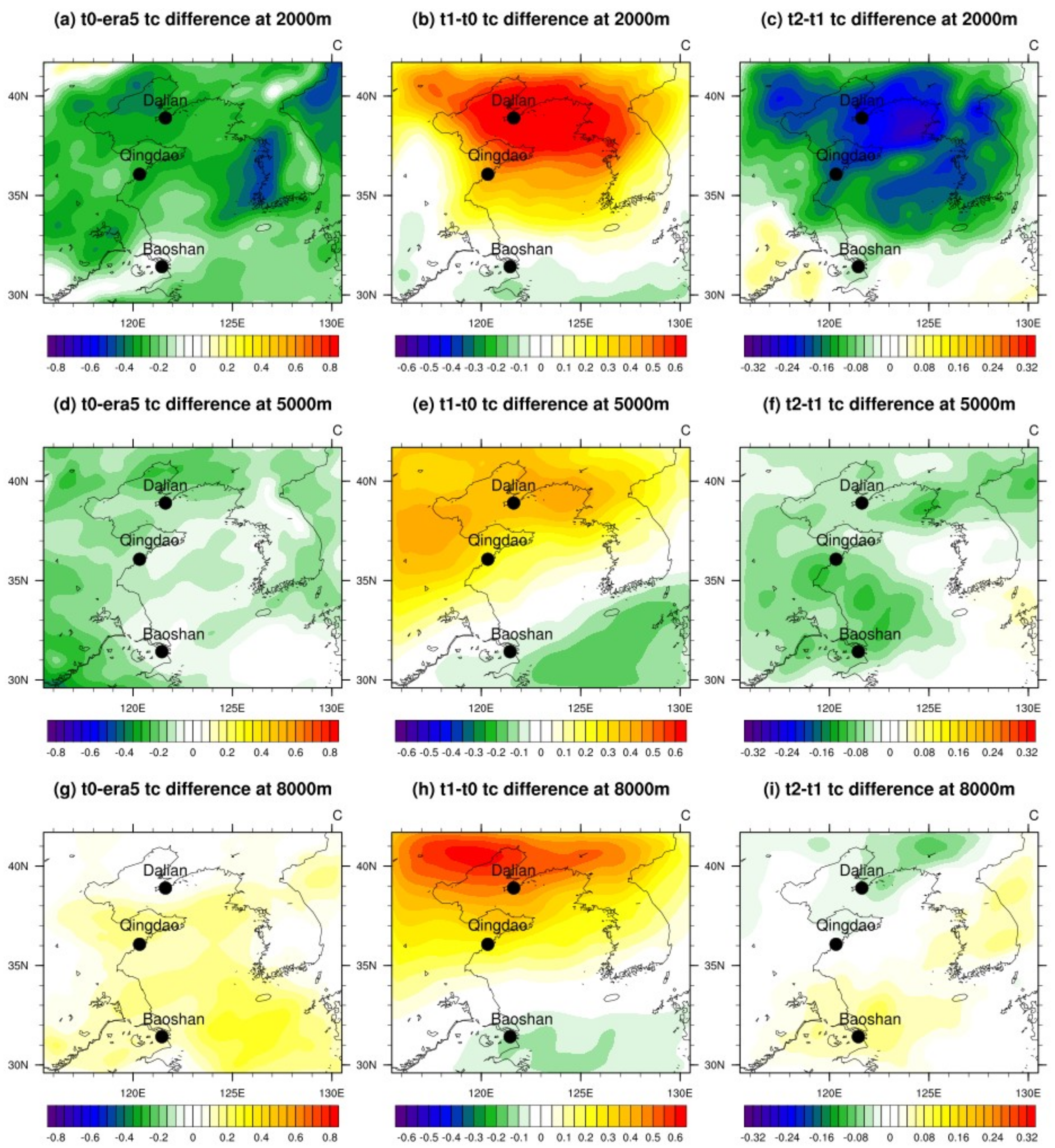
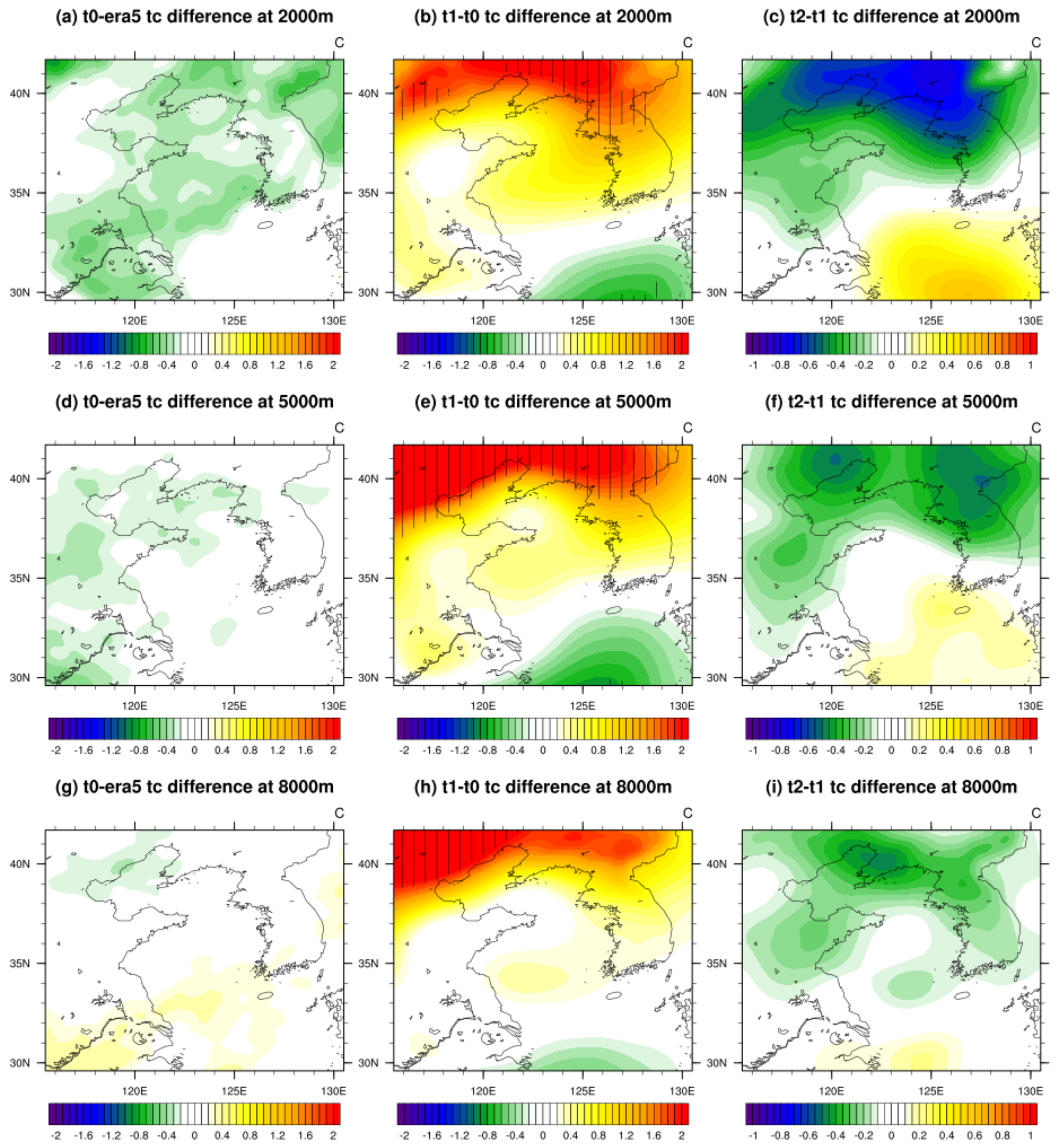
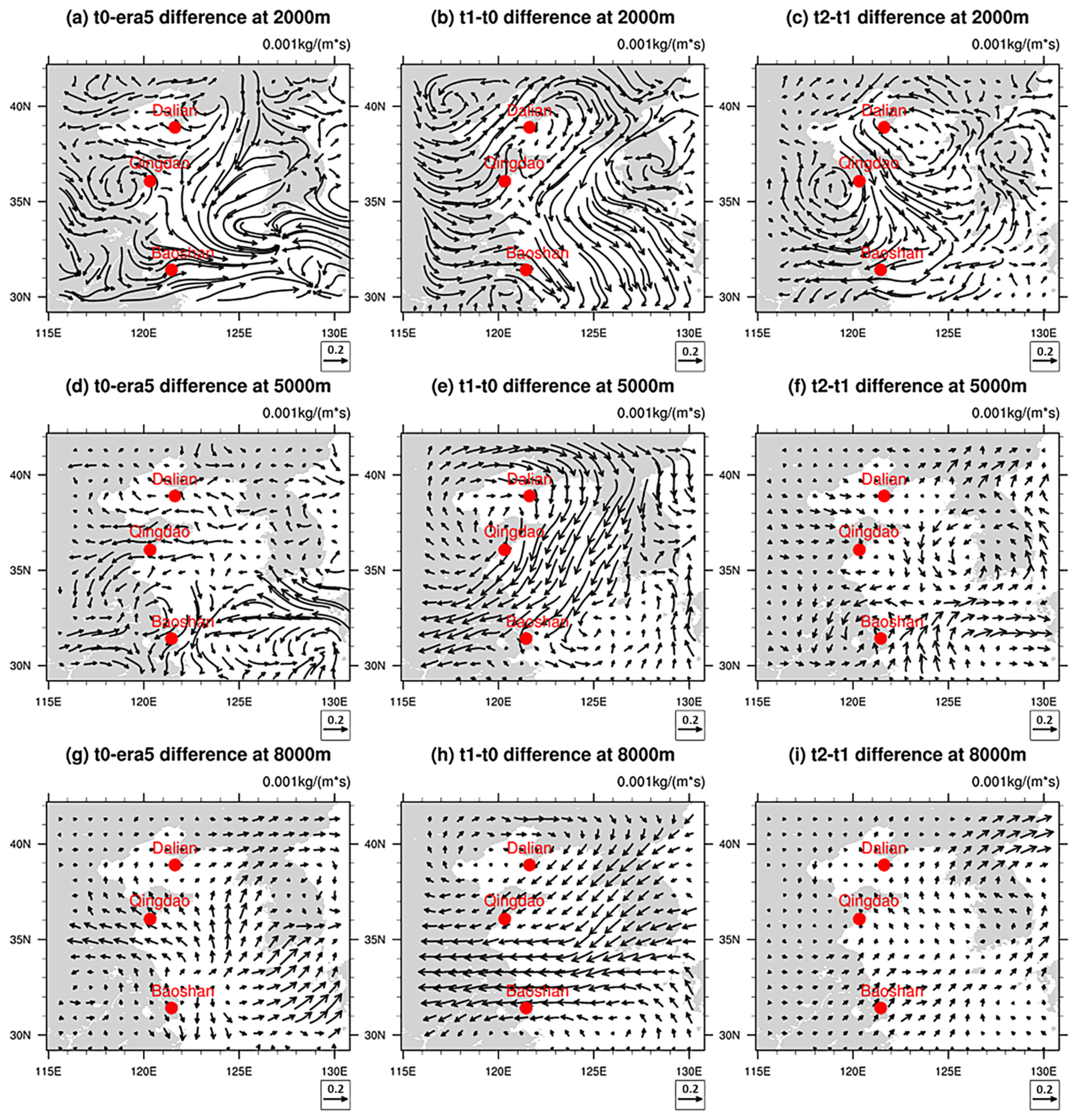
In terms of the regional bias distributions, the revised atmospheric refraction forecasts in this study were generally positively biased, and the bias was higher in the south and lower in the north. The t1 test with the inclusion of the sounding data reduced the bias of the control test over the ocean areas within the lower troposphere, but probably increased the forecasting bias at other levels with fewer data. With the addition of the COSMIC data with wider regional coverage, the t2 test weakened the increased bias of the t1 test over many areas. The most obvious correction occurred around the level of 2000 m, where the regional correction was up to 1.6 M on an average.

(6)

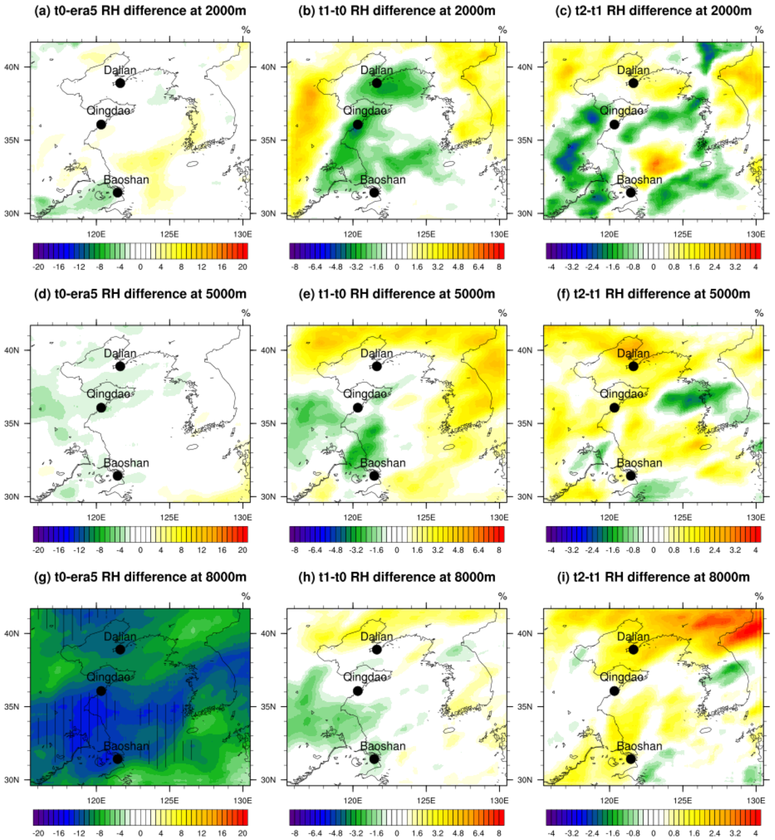
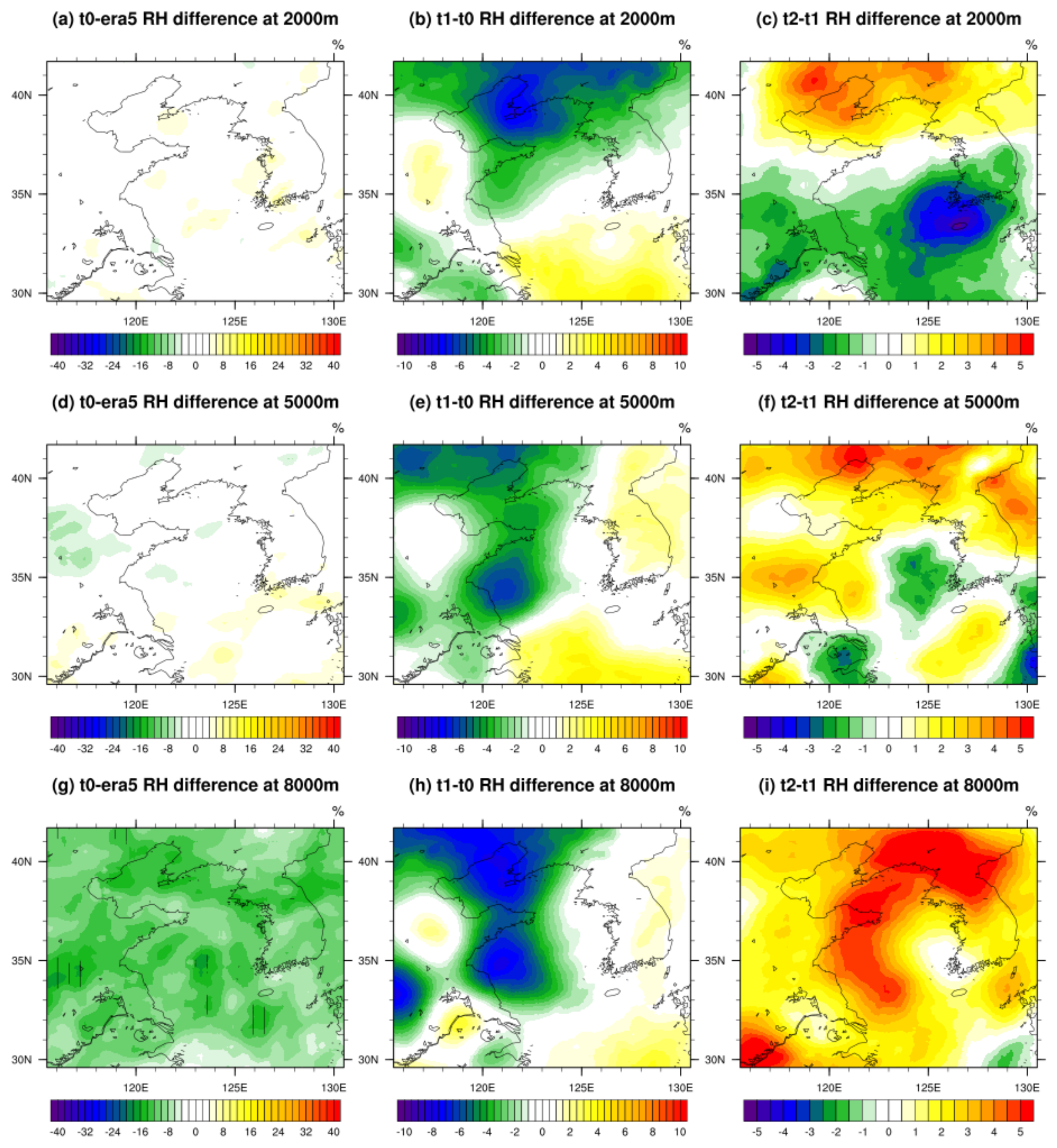
The changes in the revised atmospheric refraction due to assimilation came mainly from the changes in temperature and humidity, and rarely from the changes in air pressure. In the lower and middle troposphere, the improvements in the forecasted revised atmospheric refraction were largely dominated by the changes in humidity. The contributions of the humidity decreased with increasing altitudes. In the upper troposphere, the changes in the revised atmospheric refraction were influenced by multiple factors, including humidity and temperature.

Since this study used the 3D EnVar module, differences among the three forecasting tests were attributed to the differences in the initial humidity and temperature fields resulting from assimilation. After assimilating the sounding data, the humidity gradient between the north and south of the domain increased, while the temperature gradient decreased. The introduction of COSMIC data assimilation further weakened but did not alter the spatial distribution pattern of change. This change in temperature and humidity further caused alterations in atmospheric pressure, wind field, and water vapor transport, enabling changes from the initial field to gradually alter the spatial distribution pattern after about 12 h, ultimately affecting the distribution of revised atmospheric refraction.

References

1. Elahi, E.; Khalid, Z.; Zhang, Z. Understanding farmers’ intention and willingness to install renewable energy technology: A solution to reduce the environmental emissions of agriculture. Appl. Energy 2022, 309, 118459. [Google Scholar] [CrossRef]
2. Elahi, E.; Khalid, Z.; Tauni, M.Z.; Zhang, H.; Xing, L. Extreme weather events risk to crop production and the adaptation of innovative management strategies to mitigate the risk: A retrospective survey of rural Punjab, Pakistan. Technovation 2022, 117, 102255. [Google Scholar] [CrossRef]
3. Abbas, A.; Waseem, M.; Ahmad, R.; Khan, K.A.; Zhao, C.; Zhu, J. Sensitivity analysis of greenhouse gas emissions at farm level: Case study of grain and cash crops. Environ. Sci. Pollut. Res. 2022, 29, 82559–82573. [Google Scholar] [CrossRef]
4. Abbas, A.; Zhao, C.; Waseem, M.; Khan, K.A.; Ahmad, R. Analysis of energy input-output of farms and assessment of greenhouse gas emissions: A case study of cotton growers. Front. Environ. Sci. 2022, 9, 826838. [Google Scholar] [CrossRef]
5. Wang, Y.M.; Gao, S.H.; Fu, G.; Sun, J.L.; Zhang, S.P. Assimilating MTSAT-derived humidity in nowcasting sea fog over the Yellow Sea. Weather. Forecast. 2014, 29, 205–225. [Google Scholar] [CrossRef]
6. Chen, S.-Y.; Nguyen, T.-C.; Huang, C.-Y. Impact of radio occultation data on the prediction of typhoon Haishen (2020) with WRFDA hybrid assimilation. Atmosphere 2021, 12, 1397. [Google Scholar] [CrossRef]
7. Mueller, M.J.; Kren, A.C.; Cucurull, L.; Casey, S.P.F.; Hoffman, R.N.; Atlas, R.; Peevey, T.R. Impact of refractivity profiles from a proposed GNSS-RO constellation on tropical cyclone forecasts in a global modeling system. Mon. Weather. Rev. 2020, 148, 3037–3057. [Google Scholar] [CrossRef]
8. Feng, J.; Qin, X.; Wu, C.; Zhang, P.; Yang, L.; Shen, X.; Han, W.; Liu, Y. Improving typhoon predictions by assimilating the retrieval of atmospheric temperature profiles from the FengYun-4A’s Geostationary Interferometric Infrared Sounder (GIIRS). Atmos. Res. 2022, 280, 106391. [Google Scholar] [CrossRef]
9. Kumar, P.; Kishtawal, C.; Pal, P. Impact of satellite rainfall assimilation on Weather Research and Forecasting model predictions over the Indian region. J. Geophys. Res. Atmos. 2014, 119, 2017–2031. [Google Scholar] [CrossRef]
10. Xie, Y.; Fan, S.; Chen, M.; Shi, J.; Zhong, J.; Zhang, X. An assessment of satellite radiance data assimilation in RMAPS. Remote Sens. 2018, 11, 54. [Google Scholar] [CrossRef]
11. Zhang, B.; Wu, Y.; Zhao, B.; Chanussot, J.; Hong, D.; Yao, J.; Gao, L. Progress and challenges in intelligent remote sensing satellite systems. IEEE J. Sel. Top. Appl. Earth Obs. Remote Sens. 2022, 15, 1814–1822. [Google Scholar] [CrossRef]
12. Fang, Z.Y. The Evolution of Meteorological Satellites and the Insight from it. Adv. Meteor. Sci. Technol. 2014, 4, 27–34. (In Chinese) [Google Scholar]
13. Hajj, G.A.; Kursinski, E.R.; Romans, L.J.; Bertinger, W.I.; Leroy, S.S. A technical description of atmospheric sounding by GPS occultations. J. Atmos. Sol. Terr. Phys. 2002, 64, 451–469. [Google Scholar] [CrossRef]
14. Cucurull, L.; Kuo, Y.-H.; Barker, D.; Rizvi, S. Assessing the impact of simulated COSMIC GPS radio occultation data on weather analysis over the Antarctic: A case study. Mon. Weather. Rev. 2006, 134, 3283–3296. [Google Scholar] [CrossRef]
15. Bonafoni, S.; Biondi, R.; Brenot, H.; Anthes, R. Radio occultation and ground-based GNSS products for observing, understanding and predicting extreme events: A review. Atmos. Res. 2019, 230, 104624. [Google Scholar] [CrossRef]
16. Johnston, B.R.; Randel, W.J.; Sjoberg, J.P. Evaluation of tropospheric moisture characteristics among COSMIC-2, ERA5 and MERRA-2 in the tropics and subtropics. Remote Sens. 2021, 13, 880. [Google Scholar] [CrossRef]
17. Yamazaki, Y.; Arras, C.; Andoh, S.; Miyoshi, Y.; Shinagawa, H.; Harding, B.; Englert, C.; Immel, T.; Sobhkhiz-Miandehi, S.; Stolle, C. Examining the wind shear theory of sporadic E with ICON/MIGHTI winds and COSMIC-2 radio occultation data. Geophys. Res. Lett. 2022, 49, e2021GL096202. [Google Scholar] [CrossRef]
18. Bai, W.; Deng, N.; Sun, Y.; Du, Q.; Xia, J.; Wang, X.; Meng, X.; Zhao, D.; Liu, C.; Tan, G.; et al. Applications of GNSS-RO to Numerical Weather Prediction and Tropical Cyclone Forecast. Atmosphere 2020, 11, 1204. [Google Scholar] [CrossRef]
19. Healy, S. Assimilation of GPS radio occultation measurements at ECMWF. In Proceedings of the GRAS SAF Workshop on Applications of GPSRO Measurements; ECMWF: Reading, UK, 2008; pp. 16–18. [Google Scholar]
20. Anlauf, H.; Pingel, D.; Rhodin, A. Assimilation of GPS radio occultation data at DWD. Atmos. Meas. Tech. Discuss. 2011, 4, 1533–1554. [Google Scholar] [CrossRef]
21. Hirahara, Y.; Owada, H.; Moriya, M. Assimilation of GNSS RO data into JMA’s mesoscale NWP system. WGNE 2017, 47, 01.15–01.16. [Google Scholar]
22. Schreiner, W.S.; Weiss, J.; Anthes, R.A.; Braun, J.; Chu, V.; Fong, J.; Hunt, D.; Kuo, Y.H.; Meehan, T.; Serafino, W. COSMIC-2 radio occultation constellation: First results. Geophys. Res. Lett. 2020, 47, e2019GL086841. [Google Scholar] [CrossRef]
23. Lien, G.-Y.; Lin, C.-H.; Huang, Z.-M.; Teng, W.-H.; Chen, J.-H.; Lin, C.-C.; Ho, H.-H.; Huang, J.-Y.; Hong, J.-S.; Cheng, C.-P. Assimilation impact of early FORMOSAT-7/COSMIC-2 GNSS radio occultation data with Taiwan’s CWB Global Forecast System. Mon. Weather. Rev. 2021, 149, 2171–2191. [Google Scholar] [CrossRef]
24. Ilyas, S.Z.; Hassan, A.; Bibi, N.; Mufti, H.; Jalil, A.; Baqir, Y. Evaluation of radio refractivity in the troposphere over the big cities of Pakistan. J. Geovis. Spat. Anal. 2022, 6, 3. [Google Scholar] [CrossRef]
25. Peng, X.; Huang, W.; Li, X.; Yang, L.; Chen, F. A spatiotemporal atmospheric refraction correction method for improving the geolocation accuracy of high-resolution remote sensing images. Remote Sens. 2022, 14, 5344. [Google Scholar] [CrossRef]
26. Bean, B.R.; Dutton, E. Radio Meteorology; Superintendent of Documents, US Government Printing Office: Washington, DC, USA, 1966.
27. Tang, W.; Cha, H.; Wei, M.; Tian, B.; Ren, X. An atmospheric refractivity inversion method based on deep learning. Results Phys. 2019, 12, 582–584. [Google Scholar] [CrossRef]
28. Raju, A.; Kumar, P.; Parekh, A.; Ravi Kumar, K.; Nagaraju, C.; Chowdary, J.; Nagarjuna Rao, D. Evaluation of Upper Tropospheric Humidity in WRF Model during Indian Summer Monsoon. Asia-Pac. J. Atmos. Sci. 2019, 55, 575–588. [Google Scholar] [CrossRef]
29. Chen, S.-Y.; Liu, C.-Y.; Huang, C.-Y.; Hsu, S.-C.; Li, H.-W.; Lin, P.-H.; Cheng, J.-P.; Huang, C.-Y. An analysis study of FORMOSAT-7/COSMIC-2 radio occultation data in the troposphere. Remote Sens. 2021, 13, 717. [Google Scholar] [CrossRef]
30. Chang, C.-C.; Yang, S.-C. Impact of assimilating the Formosat-7/COSMIC-II GNSS radio occultation data on predicting the heavy rainfall event in Taiwan on August 13, 2019. Terr. Atmos. Ocean. Sci. 2022, 33, 7. [Google Scholar] [CrossRef]
31. Singh, R.; Ojha, S.P.; Anthes, R.; Hunt, D. Evaluation and assimilation of the COSMIC-2 radio occultation constellation observed atmospheric refractivity in the WRF data assimilation system. J. Geophys. Res. Atmos. 2021, 126, e2021JD034935. [Google Scholar] [CrossRef]
32. Chen, Y.-J.; Hong, J.-S.; Chen, W.-J. Impact of Assimilating FORMOSAT-7/COSMIC-2 Radio Occultation Data on Typhoon Prediction Using a Regional Model. Atmosphere 2022, 13, 1879. [Google Scholar] [CrossRef]
33. Miller, W.J.; Chen, Y.; Ho, S.-P.; Shao, X. Evaluating the Impacts of COSMIC-2 GNSS RO Bending Angle Assimilation on Atlantic Hurricane Forecasts Using the HWRF Model. Mon. Weather. Rev. 2023, 151, 1821–1847. [Google Scholar] [CrossRef]
34. Zou, J.; Zhan, C.; Song, H.; Hu, T.; Qiu, Z.; Wang, B.; Li, Z. Development and evaluation of a hydrometeorological forecasting system using the Coupled Ocean-Atmosphere-Wave-Sediment Transport (COAWST) Model. Adv. Meteorol. 2021, 2021, 6658722. [Google Scholar] [CrossRef]
35. Jiao, D.; Xu, N.; Yang, F.; Xu, K. Evaluation of spatial-temporal variation performance of ERA5 precipitation data in China. Sci. Rep. 2021, 11, 17956. [Google Scholar] [CrossRef] [PubMed]
36. Warner, J.C.; Armstrong, B.; He, R.; Zambon, J.B. Development of a coupled ocean–atmosphere–wave–sediment transport (COAWST) modeling system. Ocean. Model. 2010, 35, 230–244. [Google Scholar] [CrossRef]
37. Sian, K.T.L.K.; Dong, C.; Liu, H.; Wu, R.; Zhang, H. Effects of Model Coupling on Typhoon Kalmaegi (2014) Simulation in the South China Sea. Atmosphere 2020, 11, 432. [Google Scholar] [CrossRef]
38. Zheng, M.; Zhang, Z.; Zhang, W.; Fan, M.; Wang, H. Effects of ocean states coupling on the simulated Super Typhoon Megi (2010) in the South China Sea. Front. Mar. Sci. 2023, 10, 1105687. [Google Scholar] [CrossRef]
39. Hamill, T.M.; Snyder, C. A hybrid ensemble Kalman filter—3D variational analysis scheme. Mon. Weather. Rev. 2000, 128, 2905–2919. [Google Scholar] [CrossRef]
40. Lorenc, A.C. The potential of the ensemble Kalman filter for NWP—A comparison with 4D-Var. Q. J. Roy. Meteor. Soc. 2003, 129, 3183–3203. [Google Scholar] [CrossRef]
41. Buehner, M. Ensemble-derived stationary and flow-dependent background-error covariances: Evaluation in a quasi-operational NWP setting. Q. J. Roy. Meteor. Soc. 2005, 131, 1013–1043. [Google Scholar] [CrossRef]
42. Wang, X.; Snyder, C.; Hamill, T.M. On the theoretical equivalence of differently proposed ensemble–3DVAR hybrid analysis schemes. Mon. Weather. Rev. 2007, 135, 222–227. [Google Scholar] [CrossRef]
43. Michel, Y.; Brousseau, P. A square-root, dual-resolution 3DEnVar for the AROME Model: Formulation and evaluation on a summertime convective period. Mon. Weather. Rev. 2021, 149, 3135–3153. [Google Scholar] [CrossRef]
44. Grell, G.A.; Freitas, S.R. A scale and aerosol aware stochastic convective parameterization for weather and air quality modeling. Atmos. Chem. Phys. 2014, 14, 5233–5250. [Google Scholar] [CrossRef]
45. Hong, S.-Y.; Lim, J.-O.J. The WRF single-moment 6-class microphysics scheme (WSM6). Asia-Pac. J. Atmos. Sci. 2006, 42, 129–151. [Google Scholar]
46. Mlawer, E.J.; Taubman, S.J.; Brown, P.D.; Iacono, M.J.; Clough, S.A. Radiative transfer for inhomogeneous atmospheres: RRTM, a validated correlated-k model for the longwave. J. Geophys. Res. Atmos. 1997, 102, 16663–16682. [Google Scholar] [CrossRef]
47. Dudhia, J. Numerical study of convection observed during the winter monsoon experiment using a mesoscale two-dimensional model. J. Atmos. Sci. 1989, 46, 3077–3107. [Google Scholar] [CrossRef]
48. Hu, X.M.; Klein, P.M.; Xue, M. Evaluation of the updated YSU planetary boundary layer scheme within WRF for wind resource and air quality assessments. J. Geophys. Res. Atmos. 2013, 118, 10,490–10,505. [Google Scholar] [CrossRef]
49. Paulson, C.A. The mathematical representation of wind speed and temperature profiles in the unstable atmospheric surface layer. J. Appl. Meteorol. Clim. 1970, 9, 857–861. [Google Scholar]
50. Mellor, G.L.; Yamada, T. Development of a turbulence closure model for geophysical fluid problems. Rev. Geophys. 1982, 20, 851–875. [Google Scholar] [CrossRef]
51. Flather, R. A tidal model of the northwest European continental shelf. Mem. Soc. Roy. Sci. Liege 1976, 10, 141–164. [Google Scholar]
Figure 1. (a) Topographic map of the study area with the locations of the radiosonde stations. The study domain of the COAWST model is framed by black lines. (b) The trajectory of the COSMIC–2 satellites during September over the study domain. The trajectory lines are denoted as black lines and red date numbers. The black dots in these lines imply the locations where the satellite enters the domain, and the blue dots imply the locations for exiting.
Atmosphere 14 01776 g001
Figure 2. The box plots of revised atmospheric refraction bias for the forecasts of 24 h ahead at (a) Dalian, (b) Qingdao, and (c) Baoshan station; for the forecasts of 48 h ahead at (d) Dalian, (e) Qingdao, and (f) Baoshan station; and for the forecasts of 72 h ahead at (g) Dalian, (h) Qingdao, and (i) Baoshan station. The black, blue, and red boxes represent the bias distributions of the t0, t1, and t2 tests, respectively. The green boxes represent the difference distribution of the ERA5 reanalysis data when compared with the station sounding data.
Atmosphere 14 01776 g002
Figure 3. The profiles of revised atmospheric refraction bias versus height for the 24 h forecasts at (a) Dalian, (b) Qingdao, and (c) Baoshan station; for the 48 h forecasts at (d) Dalian, (e) Qingdao, and (f) Baoshan station; and for the 72 h forecasts at (g) Dalian, (h) Qingdao, and (i) Baoshan station. The black, blue, and red lines represent the bias profiles of the t0, t1, and t2 tests, respectively. The green lines represent the difference profiles of the ERA5 reanalysis data when compared with the station sounding data.
Atmosphere 14 01776 g003
Figure 4. The profiles of revised atmospheric refraction bias versus time during the test period for the 24 h forecasts of the t0 test at (a) Dalian, (b) Qingdao, and (c) Baoshan station; of the t1 test at (d) Dalian, (e) Qingdao, and (f) Baoshan station; and of the t2 test at (g) Dalian, (h) Qingdao, and (i) Baoshan station. The profiles of revised atmospheric refraction difference versus time for the ERA5 compared with sounding data at (j) Dalian, (k) Qingdao, and (l) Baoshan station.
Atmosphere 14 01776 g004
Figure 5. The spatial distributions of the differences in the revised atmospheric refraction from (a) t0 minus era5, (b) t1 minus t0, and (c) t2 minus t1 at the height of 2000 m; from (d) t0 minus era5, (e) t1 minus t0, and (f) t2 minus t1 at the height of 5000 m, and from (g) t0 minus era5, (h) t1 minus t0; and (i) t2 minus t1 at the height of 8000 m. The three black dots represent the locations of Dalian, Qingdao, and Baoshan stations. The areas shaded by strips represent the difference there passed the significance test at a 95% confidence level.
Atmosphere 14 01776 g005
Figure 6. The spatial distributions of the differences in relative humidity from (a) t0 minus era5, (b) t1 minus t0, and (c) t2 minus t1 at the height of 2000m; from (d) t0 minus era5, (e) t1 minus t0, and (f) t2 minus t1 at the height of 5000 m; and from (g) t0 minus era5, (h) t1 minus t0, and (i) t2 minus t1 at the height of 8000 m. The three black dots represent the locations of the Dalian, Qingdao, and Baoshan stations. The areas shaded by strips represent the difference there passed the significance test at a 95% confidence level.
Atmosphere 14 01776 g006
Figure 7. The spatial distributions of the differences in air temperature from (a) t0 minus era5, (b) t1 minus t0, and (c) t2 minus t1 at the height of 2000 m; from (d) t0 minus era5, (e) t1 minus t0, and (f) t2 minus t1 at the height of 5000 m; and from (g) t0 minus era5, (h) t1 minus t0, and (i) t2 minus t1 at the height of 8000 m. The three black dots represent the locations of the Dalian, Qingdao, and Baoshan stations.
Atmosphere 14 01776 g007
Figure 8. The profiles of relative humidity assimilated in the t1 and t2 test at (a) Dalian, (b) Qingdao, and (c) Baoshan station; and of air temperature assimilated in the t1 and t2 test at (d) Dalian, (e) Qingdao, and (f) Baoshan station. The blue lines represent the mean profiles of sounding data at 00:00 UTC, and the red scatters represent the COSMIC–2 data during the three hours before and after 00:00 UTC every day.
Atmosphere 14 01776 g008
Figure 9. The spatial distributions of the differences in the initial relative humidity fields at 00:00 UTC from (a) t0 minus era5, (b) t1 minus t0, and (c) t2 minus t1 at the height of 2000 m; from (d) t0 minus era5, (e) t1 minus t0, and (f) t2 minus t1 at the height of 5000 m; and from (g) t0 minus era5, (h) t1 minus t0, and (i) t2 minus t1 at the height of 8000 m. The areas shaded by strips represent the difference there passed the significance test at a 95% confidence level.
Atmosphere 14 01776 g009
Figure 10. The spatial distributions of the differences in the initial temperature fields at 00:00 UTC from (a) t0 minus era5, (b) t1 minus t0, and (c) t2 minus t1 at the height of 2000 m; from (d) t0 minus era5, (e) t1 minus t0, and (f) t2 minus t1 at the height of 5000 m; and from (g) t0 minus era5, (h) t1 minus t0, and (i) t2 minus t1 at the height of 8000 m. The areas shaded by strips represent the difference there passed the significance test at a 95% confidence level.
Atmosphere 14 01776 g010
Figure 11. The spatial distributions of the differences in water vapor flux from (a) t0 minus era5, (b) t1 minus t0, and (c) t2 minus t1 at the height of 2000 m; from (d) t0 minus era5, (e) t1 minus t0; and (f) t2 minus t1 at the height of 5000 m, and from (g) t0 minus era5, (h) t1 minus t0, and (i) t2 minus t1 at the height of 8000 m. The three red dots represent the locations of the Dalian, Qingdao, and Baoshan stations.
Atmosphere 14 01776 g011