Predicting and Reconstructing Aerosol–Cloud–Precipitation Interactions with Physics-Informed Neural Networks

Abstract

Interactions between clouds, aerosol, and precipitation are crucial aspects of weather and climate. The simple Koren–Feingold conceptual model is important for providing deeper insight into the complex aerosol–cloud–precipitation system. Recently, artificial neural networks (ANNs) and physics-informed neural networks (PINNs) have been used to study multiple dynamic systems. However, the Koren–Feingold model for aerosol–cloud–precipitation interactions has not yet been studied with either ANNs or PINNs. It is challenging for pure data-driven models, such as ANNs, to accurately predict and reconstruct time series in a small data regime. The pure data-driven approach results in the ANN becoming a “black box” that limits physical interpretability. We demonstrate how these challenges can be overcome by combining a simple ANN with physical laws into a PINN model (not purely data-driven, good for the small data regime, and interpretable). This paper is the first to use PINNs to learn about the original and modified Koren–Feingold models in a small data regime, including external forcings such as wildfire-induced aerosols or the diurnal cycle of clouds. By adding external forcing, we investigate the effects of environmental phenomena on the aerosol–cloud–precipitation system. In addition to predicting the system’s future, we also use PINN to reconstruct the system’s past: a nontrivial task because of time delay. So far, most research has focused on using PINNs to predict the future of dynamic systems. We demonstrate the PINN’s ability to reconstruct the past with limited data for a dynamic system with nonlinear delayed differential equations, such as the Koren–Feingold model, which remains underexplored in the literature. The main reason that this is possible is that the model is non-diffusive. We also demonstrate for the first time that PINNs have significant advantages over traditional ANNs in predicting the future and reconstructing the past of the original and modified Koren–Feingold models containing external forcings in the small data regime. We also show that the accuracy of the PINN is not sensitive to the value of the regularization factor ($\lambda$), a key parameter for the PINN that controls the weight for the physics loss relative to the data loss, for a broad range (from $\lambda =1\times {10}^3$ to $\lambda =1\times {10}^5$).

1. Introduction

1.1. Aerosol–Cloud–Precipitation System

Aerosol–cloud interactions have important influences on weather, climate, and their predictability [1]. Clouds serve as a source of precipitation and storms. Rain can form when cloud water is converted to rainwater. Factors such as aerosol particle concentration, warm cloud depth, and cloud droplet concentration affect the rate of conversion of cloud water to rainwater [2]. Additionally, clouds reflect radiation from the sun, regulating the solar radiation absorbed by the earth. Therefore, it is crucial to predict and understand aerosol–cloud interactions. However, this task is challenging because clouds are nonlinear dynamic systems with many degrees of freedom [3]. It is also understood that aerosol affects cloud depth, though it is not easy to quantify the effects [4]. Water droplet condensation on aerosol nuclei leads to cloud formation. Usually, higher aerosol concentrations result in higher cloud droplet concentrations [5], increasing the optical thickness and reflective ability of clouds and creating a stronger cooling effect by reflecting more solar radiation [6,7].

Complex and detailed models, such as large eddy simulations, are used to make predictions from an aerosol–cloud–precipitation system [8]. However, these models are computationally expensive, so the aerosol–cloud–precipitation system has been simplified with the Koren–Feingold conceptual model to improve our understanding of the major features of the system’s underlying physical mechanisms, particularly for shallow clouds [1]. This idealized model treats the aerosol–cloud–precipitation system as a predator–prey problem, with rain as the predator and clouds as the prey, modulated by aerosol or the related cloud droplet concentration. According to the delayed differential equations in the Koren–Feingold model, cloud depth, cloud droplet concentration, and rainfall exhibit oscillations. The use of simpler models to represent aerosol–cloud–precipitation interactions produces a better grasp of the underlying physics of these interactions and highlights predictable elements of a more complex system.

Wildfires are a major source of aerosols and can thus affect the cloud–precipitation system [9]. Aerosols from wildfire smoke have been a significant source of uncertainty for climate prediction [10]. Wildfires release biomass-burning aerosols that act as cloud condensation nuclei and affect cloud formation and precipitation [11]. It is important to understand how the aerosol pollution induced by environmental phenomena, such as wildfires, affects the aerosol–cloud–precipitation system. Recent studies have focused on using observational data to study the impacts of aerosol pollution on the cloud–precipitation system [12,13,14,15], but it could also be fruitful to study these impacts through the Koren–Feingold conceptual model.

Another external forcing that can be studied with the Koren–Feingold model is a diurnal radiative forcing on cloud depth. This diurnal cycle has been observed and examined in several studies [16,17,18,19,20]. This cycle occurs because surface temperatures vary as the earth is warmed during the daytime and cooled during the nighttime [21,22]. These changes in surface temperature affect the convection that forms clouds and result in cloud depths varying cyclically over the course of a day, with more low clouds appearing in the afternoon [20]. The diurnal cycle of low-level clouds is related to their ability to reflect radiation [16]. Accounting for external phenomena, such as the diurnal radiative forcing cycle, in the simple Koren–Feingold conceptual model offers an insightful and useful way to deepen our understanding of the effect of such phenomena on the aerosol–cloud–precipitation system.

1.2. Artificial Neural Network and Physics-Informed Neural Networks

Although artificial neural networks (ANNs) have already been used to analyze a wide range of dynamic systems, e.g., [23,24,25,26], they have not been used to study the Koren–Feingold conceptual system for aerosol–cloud–precipitation interactions. ANNs are able to learn complex, nonlinear relationships and perform particularly well with large datasets. However, this pure data-driven approach results in the ANN becoming a “black box” that limits physical interpretability. Furthermore, the lack of data in certain fields limits the applicability of ANNs in those fields in the small data regime, as large datasets are difficult and expensive to obtain.

Other advanced hybrid models recently used for time series modelling similarly rely on large datasets to be more successful [27,28,29,30,31,32,33,34]. For example, the advanced hybrid deep learning model combining a long short-term memory neural network with an ant–lion optimizer model (LSTM-ALO) can successfully predict monthly river runoff using 336 months of training data [27]. In this case, the total time interval covering the training data (336 months) is significantly longer than the prediction time interval (1 month), and there is a 336:1 ratio between them. Another advanced hybrid deep learning model combining the random vector functional link with a water cycle optimization algorithm and a moth–flame optimization algorithm (RVFL-WCAMFO) trained on 18 years of monthly data successfully predicted monthly air temperature [33]. The periodicity (seasonal cycle) revealed by the training dataset can also significantly improve the accuracy of the predictions [33]. Once again, the total time interval spanning the training data (216 months) is much longer than the prediction time interval (1 month), i.e., there is a 216:1 ratio between them. The training data are long enough for the model to learn the periodicity. Similarly, an advanced hybrid deep learning model combining a single vector machine and firefly algorithm–particle swarm optimization (SVM-FFAPSO) with a training dataset of 3727 daily data successfully predicted daily dissolved oxygen levels [31]. The ratio of the total time interval of the training data and the prediction time interval is 3727:1. The above-mentioned pure data-driven models depend on large training datasets and are commonly used for large data problems.

Our study focuses on a small data regime with limited training data, where the ratio between the total time interval of the training data and the prediction/reconstruction time interval is close to 1:1. In this small data regime, there are insufficient data to train advanced hybrid deep learning models for prediction and reconstruction. Therefore, the problem addressed in this study differs fundamentally from those addressed in the above studies using advanced hybrid deep learning models and large training datasets. Our study requires a different approach that focuses on the role of physical laws in aiding future predictions and past reconstructions in small data regimes. Physics-informed neural networks (PINNs) allow for prior knowledge (such as differential equations that govern a system) to be combined with data, which is especially helpful in small data regimes where data are limited but the system is regulated by physical laws [35]. The advantages of the PINN are its ability to learn from small, limited training data and its interpretability, because it is informed by physical laws and is not purely data-driven [35]. PINNs can generalize well and find patterns even with limited data [36,37,38]. A deep learning model that combines physical laws and data performs better than some conventional numerical models using data assimilation [39]. PINNs have already been used in fields such as biochemistry [40], hydrogeology [41], and astronomy [42]. They are also frequently used to solve ordinary and partial differential equations [43,44]. However, PINNs have not yet been applied to the conceptual Koren–Feingold model, which consists of nonlinear delayed differential equations. Also underexplored is the PINN’s ability to reconstruct the past in a small data regime with delayed differential equations. Most research focuses on using PINNs to predict the future or to estimate the features of a system based on small datasets [35,45,46].

Additionally, our study also explores the impact of time-varying external forcings on the conceptual Koren–Feingold model. These time-varying external forcings over the prediction and reconstruction time domains cannot be successfully learned by pure data-driven models over the small time interval of the training time domain. The PINN is able to incorporate the knowledge of the time-varying external forcings. Thus, it has an important advantage over pure data-driven models when predicting and reconstructing aerosol–cloud–precipitation interactions from the Koren–Feingold model with added time-varying external forcings.

1.3. Goals

In this study, we investigate whether PINNs can successfully learn the conceptual Koren–Feingold model and improve upon ANN performance in a small data regime where the ratio between the total time interval of the training data and the prediction/reconstruction time interval is close to 1:1. The main purpose of our paper is to investigate whether the combination of a simple ANN and a physical model will produce a PINN model that is much more accurate in predictive and reconstructive modes in a small data regime. Hence, we use a pure data-driven ANN (without a physical model) as the benchmark for our PINN. In particular, we explore the novel question of whether PINNs are able to reconstruct the Koren–Feingold model’s past as well as make predictions about the future in a small data regime. Using traditional methods, it is nontrivial to reconstruct the past of a system regulated by differential equations with a time delay, so advancements could be made in this area by using PINNs. Additionally, we modify the Koren–Feingold conceptual model to include time-varying external forcings such as wildfire-induced aerosols or the diurnal cycle of cloud depth. We explore the respective impacts of externally forced aerosols and the diurnal cycle of cloud depth on the aerosol–cloud–precipitation system and whether PINNs are able to perform well when external forcing is added to the conceptual Koren–Feingold model.

2. Materials and Methods

2.1. The Simple Conceptual Model for the Aerosol–Cloud–Precipitation System

The Koren–Feingold conceptual model of delayed differential equations is described as follows [1]:

$$H^{\prime }\left(t\right)=\frac{H_{max}-H\left(t\right)}{{\tau }_1}-\frac{R\left(t\right)}{c_{1}H(t-T)}=\frac{H_{max}-H\left(t\right)}{{\tau }_1}-\frac{\alpha }{c_1}\frac{H^2(t-T)}{N(t-T)}$$

(1)

$$N^{\prime }\left(t\right)=\frac{N_{max}-N\left(t\right)}{{\tau }_2}-c_{2}N\left(t-T\right)R\left(t\right)=\frac{N_{max}-N\left(t\right)}{{\tau }_2}-\alpha c_2{H}^3(t-T)$$

(2)

$$R\left(t\right)=\frac{\alpha H^3(t-T)}{N(t-T)}$$

(3)

In this system, $H\left(t\right)$ is cloud depth in meters, $N\left(t\right)$ is cloud droplet concentration in $\mathrm{c}{\mathrm{m}}^{-3}$, and $R\left(t\right)$ is precipitation in $\mathrm{m}\mathrm{m}/\mathrm{d}\mathrm{a}\mathrm{y}$. The system has a time delay of $T$ minutes, representing the delay of $R\left(t\right)$ relative to cloud depth and cloud droplet concentration caused by the time taken to form precipitation. According to the Koren–Feingold model, precipitation increases nonlinearly with cloud depth and decreases with cloud droplet concentration with the time delay $T,$ which has been confirmed through observation as well as theory [47,48]. Since $R\left(t\right)$ also causes $H\left(t\right)$ and $N\left(t\right)$ to decrease, the time delay $T$ appears in the equations of $H^{\prime }\left(t\right)$ and $N^{\prime }\left(t\right)$. $H_{max}$ is the maximum potential for cloud depth and $N_{max}$ is the maximum achievable cloud droplet concentration, that is, the background aerosol concentration. Here, ${\tau }_1$ and ${\tau }_2$ are characteristic time constants measured in minutes that regulate the exponential approach of $H\left(t\right)$ to $H_{max}$ and $N\left(t\right)$ to $N_{max}$, respectively, and $c_1$, $c_2$, and $\alpha$ are coefficients for the aerosol–cloud–precipitation interactions. Similar to the values used in the paper by Koren and Feingold [1], this study utilizes $H_{max}=530\mathrm{m}$, $N_{max}=180\mathrm{c}{\mathrm{m}}^{-3}$ without the diurnal cycle of cloud depth and $N_{max}=250\mathrm{c}{\mathrm{m}}^{-3}$ with the diurnal cycle of cloud depth, $T=24$ min, ${\tau }_1=60$ min, ${\tau }_2=60$ min, $\alpha =2\mathrm{m}\mathrm{m}{\mathrm{m}}^{-6}{\mathrm{d}\mathrm{a}\mathrm{y}}^{-1}$, $c_1=2\times {10}^{-6}\mathrm{m}\mathrm{m}{\mathrm{m}}^{-2}$, and $c_2=3\times {10}^4{\mathrm{m}}^{-1}$. The initial cloud depth is $H_0=200\mathrm{m}$ and the initial cloud droplet concentration is $N_0=50{\mathrm{cm}}^{-3}$ for $0\le t\le T$.

In this study, we use Mathematica NDSolve [49] to numerically solve the nonlinear delayed differential equations of the Koren–Feingold model [50] and to provide a truth to evaluate the performance of ANNs and PINNs when learning the conceptual model. Mathematica is a widely used mathematical computation software and has been applied successfully to aerosol-related research, e.g., [51,52,53,54].

2.2. Adding External Forcing to the Koren–Feingold Model

Additionally, we modify the Koren–Feingold model to study the effects of external forcing on the aerosol–cloud–precipitation system. We evaluate ANN and PINN performance when the aerosol–cloud–precipitation system experiences external forcing such as wildfire-induced aerosols or the diurnal cycle of clouds. The study represents the rapid increase in wildfire-induced aerosols as:

$$N_{wildfire}\left(t\right)=100(1-\cos \left(\frac{\pi }{750}t\right))\hspace{1em}\hspace{1em}\mathrm{for}t\le 1500\mathrm{m}\mathrm{i}\mathrm{n}$$

(4)

This equation idealizes the increase in background aerosol concentration that peaks at $t=750$ min and returns to the original $N_{max}$ value after 1500 min, in a similar manner to a pulse of anomalous external aerosol induced by wildfire smoke. The modified differential equation for cloud droplet concentration including the increase in the background cloud droplet concentration caused by wildfire induced aerosols becomes:

$$H^{\prime }\left(t\right)=\frac{N_{max}+N_{wildfire}\left(t\right)-N\left(t\right)}{{\tau }_2}-a{c}_{2}H(t-T{)}^3$$

(5)

Another idealization can be written to represent the diurnal cycle’s effects on the maximum potential for cloud depth in the environment:

$$H_{diurnal}\left(t\right)=50\sin \left(\frac{\pi }{720}t\right)$$

(6)

Here the sine function is chosen to represent the periodic nature of the diurnal cycle, with a period of 1440 min, or 24 h, as the diurnal cycle repeats every 24 h. The closeness of periods of 1500 min in Equation (4) and 1440 min in Equation (6) is serendipitous. The modified differential equation for the cloud depth with the diurnal cycle becomes the following equation:

$$H^{\prime }\left(t\right)=\frac{H_{max}+H_{diurnal}\left(t\right)-H\left(t\right)}{{\tau }_1}-\frac{\alpha }{c_1}\frac{H(t-T{)}^2}{N(t-T)}$$

(7)

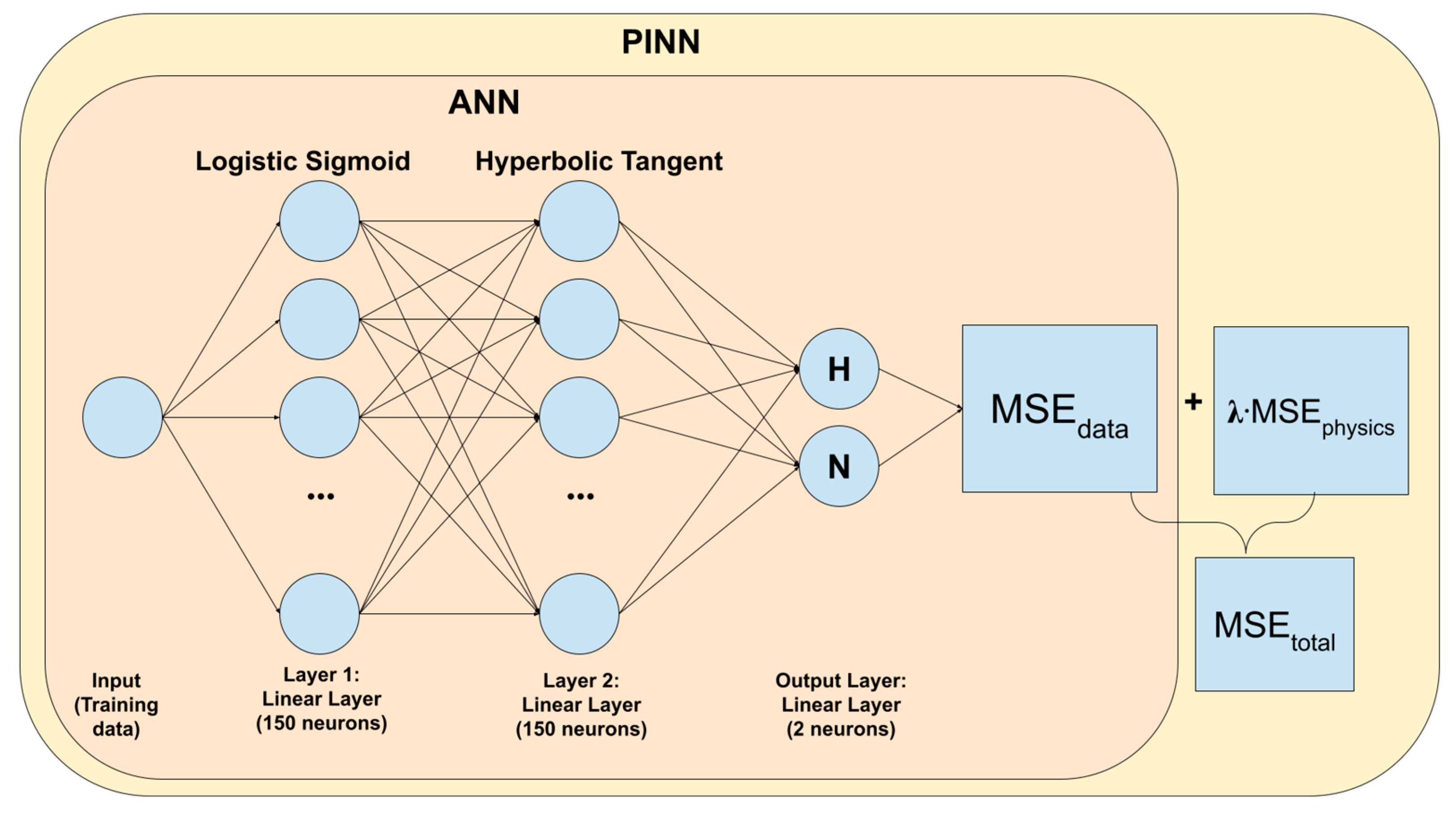
2.3. Artificial Neural Networks (ANNs) and Mean Squared Error (MSE) Loss

ANNs are made of input layers, output layers, and multiple intermediary hidden layers of data-processing neurons regulated by weights and biases [23,55]. In between the neuron layers are activation functions that decide the outputs of the neurons and help the neural network perform tasks more complicated than linear regression. The ANN is evaluated through a loss function, and it attempts to optimize weights and biases to result in the lowest loss. The loss function we use in this study is the mean squared error (MSE) loss function, which measures the average squared difference between the dataset and the neural network’s outputs using the following formula:

$$MS{E}_{data}=\frac{1}{n_{data}}\sum _{i=1}^{n_{data}}(H\left(t_i\right)-\widehat{H}\left(t_i\right){)}^2+\frac{1}{n_{data}}\sum _{i=1}^{n_{data}}(N\left(t_i\right)-\widehat{N}(t_i){)}^2$$

(8)

where ${H(t}_i)$ is the cloud depth predicted by the ANN at time $t_i$ in the data time domain, ${\widehat{H}(t}_i)$ is the true cloud depth at time $t_i$ in the data time domain, ${N(t}_i)$ is the cloud droplet concentration predicted by the ANN at time $t_i$ in the data time domain, ${\widehat{N}(t}_i)$ is the true cloud droplet concentration at time $t_i$ in the data time domain, and $n_{data}$ is the number of available data samples.

2.4. Physics-Informed Neural Networks (PINNs) and Physics Loss

PINNs were first introduced by Raissi et al. [35]. In addition to calculating loss based on data, PINNs also calculate loss based on physics principles and equations. The total loss that the PINN attempts to minimize is the sum of the data loss and the physics loss:

$$MS{E}_{total}=MS{E}_{data}+\lambda MS{E}_{physics}$$

(9)

where $MS{E}_{data}$ is the loss associated with the dataset and $MS{E}_{physics}$ is the loss associated with the differential equations of the Koren–Feingold model. Here, $\lambda$ is a regularization factor that scales the physics loss. In this study, we used $\lambda =1\times {10}^4$ because the order of magnitude of the physics loss is much smaller than that of the data loss (see Section 3.4). This value is chosen because it makes data and physics losses comparable in magnitude. With comparable data and physics losses, the PINN will attempt to minimize both while training without one loss dominating the other, as we show later in Section 3.5. If the regularization factor is too low, the PINN will not sufficiently minimize the physics loss, and if the regularization factor is too high, the PINN will not sufficiently fit to the training data and minimize the data loss (shown in Section 3.5).

The physics losses are calculated using the following equations:

$$MS{E}_{physics}=MS{E}_{physics}^H+MS{E}_{physics}^N$$

(10)

$$MS{E}_{physics}^H=\frac{1}{n_{physics}}{\sum }_{j=1}^{n_{physics}}(H^{\prime }\left(t_j\right)-\frac{H_{max}-H\left(t_j\right)}{{\tau }_1}+\frac{a}{c_1}\frac{H(t_j-T{)}^2}{N\left(t_j-T\right)}{)}^2$$

(11)

$$MS{E}_{physics}^N=\frac{1}{n_{physics}}\sum _{j=1}^{n_{physics}}(N^{\prime }\left(t_j\right)-\frac{N_{max}-N\left(t_j\right)}{{\tau }_2}+a{c}_{2}H(t_j-T{)}^3{)}^2$$

(12)

$H\left(t_j\right)$ is the cloud depth predicted by the PINN at time $t_j$ in the physics time domain, $N\left(t_j\right)$ is the cloud droplet concentration predicted by the PINN at time $t_j$ in the physics time domain, and $n_{physics}$ is the number of points in the physics time domain. It is unnecessary for the PINN to include initial conditions $H_0$ and $N_0$ because of the presence of the truth data.

With the addition of external forcing to represent the increase in maximum achievable cloud droplet concentration due to wildfire-induced aerosols, $N^{\prime }\left(t\right)$ is adjusted according to Equation (5) and the physics loss for the cloud droplet concentration becomes:

$$MS{E}_{physics}^N=\frac{1}{n_{physics}}\sum _{j=1}^{n_{physics}}(N^{\prime }\left(t_j\right)-\frac{N_{max}+N_{wildfire}\left(t_j\right)-N\left(t_j\right)}{{\tau }_2}+a{c}_{2}H(t_j-T{)}^3{)}^2$$

(13)

where

$$N_{wildfire}\left(t\right)=100(1-\cos \left(\frac{\pi }{750}t\right))\mathrm{for}t\le 1500\mathrm{m}\mathrm{i}\mathrm{n}$$

(14)

With the addition of a diurnal radiative forcing cycle of clouds affecting cloud depth, $H^{\prime }\left(t\right)$ is adjusted according to Equation (7) and the physics loss for cloud depth becomes:

$$MS{E}_{physics}^H=\frac{1}{n_{physics}}\sum _{j=1}^{n_{physics}}(H^{\prime }\left(t_j\right)-\frac{H_{max}+H_{diurnal}\left(t_j\right)-H\left(t_j\right)}{{\tau }_1}+\frac{a}{c_1}\frac{H(t_j-T{)}^2}{N\left(t_j-T\right)}{)}^2$$

(15)

where

$$H_{diurnal}\left(t\right)=50\sin \left(\frac{\pi }{720}t\right)$$

(16)

2.5. Description of Neural Network Structure and Training

In this study, we used Mathematica to create and train the ANN and PINN. The hidden layers of the ANN are composed of a 150-neuron linear layer activated by the logistic sigmoid activation function. The first layer is connected to a second 150 neuron linear layer activated by the hyperbolic tangent activation function, connected to a 2-neuron linear layer (Figure 1). The ANN trains only on data without physics for $4\times {10}^5$ rounds. However, it is important to note that after the ANN is trained for about $1\times {10}^5$ rounds, its data loss is no longer sensitive to the round number, and further training only results in a slight decrease in the ANN’s data loss. Training beyond $4\times {10}^5$ rounds does not significantly improve ANN performance.

The PINN is trained to minimize total loss, which is the sum of the data loss and the physics loss (Figure 1 and Equation (9)). The weights and biases of each linear layer are shared while the PINN is training. The initial weights and biases of each linear layer of the PINN are taken from the trained ANN. Finally, the trained neural network is extracted for the prediction and reconstruction task. In this study, the PINN is also trained for $4\times {10}^5$ rounds. With Mathematica, we used finite differentiation over a very small time interval of 0.1 min in the PINN for calculating the derivative terms of the physics loss. We also used the ADAM optimizer to minimize the training loss of both the ANN and PINN.

Both the ANN and PINN were trained on cloud depth and cloud droplet concentration truth data. The truth data were normalized by a factor of two to accelerate the ANN training process. For the future prediction, the truth dataset used for training was taken every 4.8 min between $T$ and $T_{max}/2$($T_{max}=600$ min) for a total of 58 datapoints. The models then predicted cloud depth and cloud droplet concentration from $T_{max}/2$ to $T_{max}$. The PINN was simultaneously trained to minimize the physics loss measured on the physics domain, which was every 10 min for the entire time range, from $T$ to $T_{max}$, for a total of 58 datapoints for the prediction.

For the past reconstruction, the truth dataset used for training was taken every 5 min between $T_{max}-300$ and $T_{max}$ ($T_{max}=750$ min), for a total of 61 datapoints. The models then reconstructed the cloud depth and cloud droplet concentration from $T_{max}-600$ to $T_{max}-300$. The PINN was simultaneously trained to minimize the physics loss measured in the physics domain, which was every 10 min for the entire time range, from $T_{max}-600$ to $T_{max}$, for a total of 61 datapoints for the reconstruction. Here, the time interval of the training datasets is comparable to the prediction/reconstruction time intervals (~300 min), and thus their ratio is close to 1:1.

2.6. Evaluation of Predictions and Reconstructions

MSE is widely used in other PINN studies, e.g., [35,36,41]. To be consistent with these previous studies and to allow for comparisons, we employed MSE (rather than other indices) in this study as the performance/loss index as well as the definition of the physics loss.

The predictions and reconstructions of the ANN and the PINN were evaluated with MSE loss for predicted/reconstructed cloud depth and cloud droplet concentration via the following equations:

$$MS{E}_{testdata}^H=\frac{1}{n_{testdata}}\sum _{i=1}^{n_{testdata}}(H\left(t_i\right)-\widehat{H}(t_i){)}^2$$

(17)

$$MS{E}_{testdata}^N=\frac{1}{n_{testdata}}\sum _{i=1}^{n_{testdata}}(N\left(t_i\right)-\widehat{N}(t_i){)}^2$$

(18)

where ${H(t}_i)$ is the cloud depth predicted by the ANN/PINN at time $t_i$, ${\widehat{H}(t}_i)$ is the true cloud depth at time $t_i$, ${N(t}_i)$ is the cloud droplet concentration predicted by the ANN/PINN at time $t_i$, ${\widehat{N}(t}_i)$ is the true cloud droplet concentration at time $t_i$. Here, $n_{testdata}$ is the number of test data points over the prediction/reconstruction time domain taken every 10 min, which is 31 points for the future prediction and past reconstruction.

The PINN’s physics loss for the predicted/reconstructed cloud depth and cloud droplet concentration were also calculated, respectively, using Equations (11)–(16), but only for the physics domain over the prediction/reconstruction time periods, which includes 30 physics domain points for future predictions and 31 physics domain points for past reconstructions.

3. Results

3.1. Experiments without External Forcing

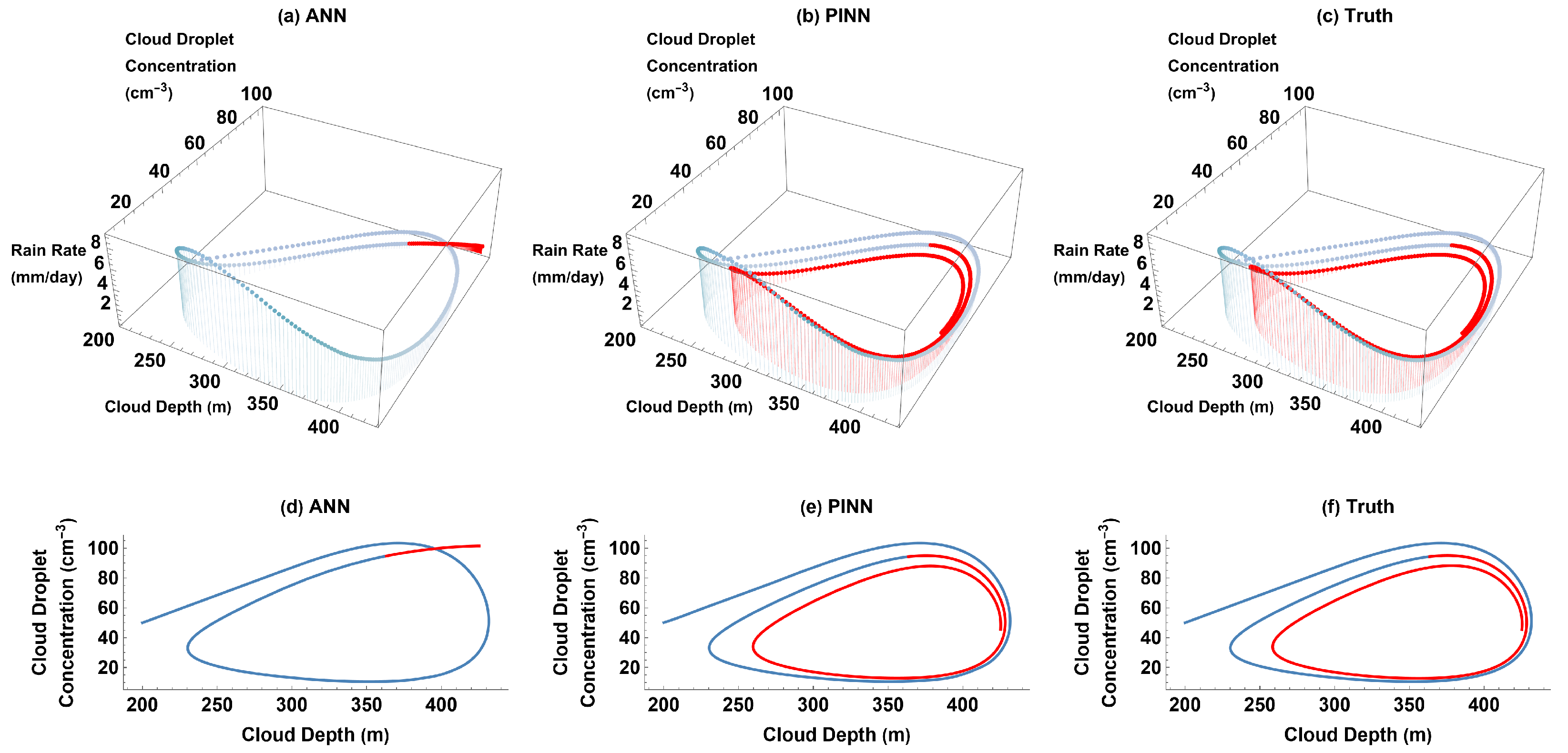
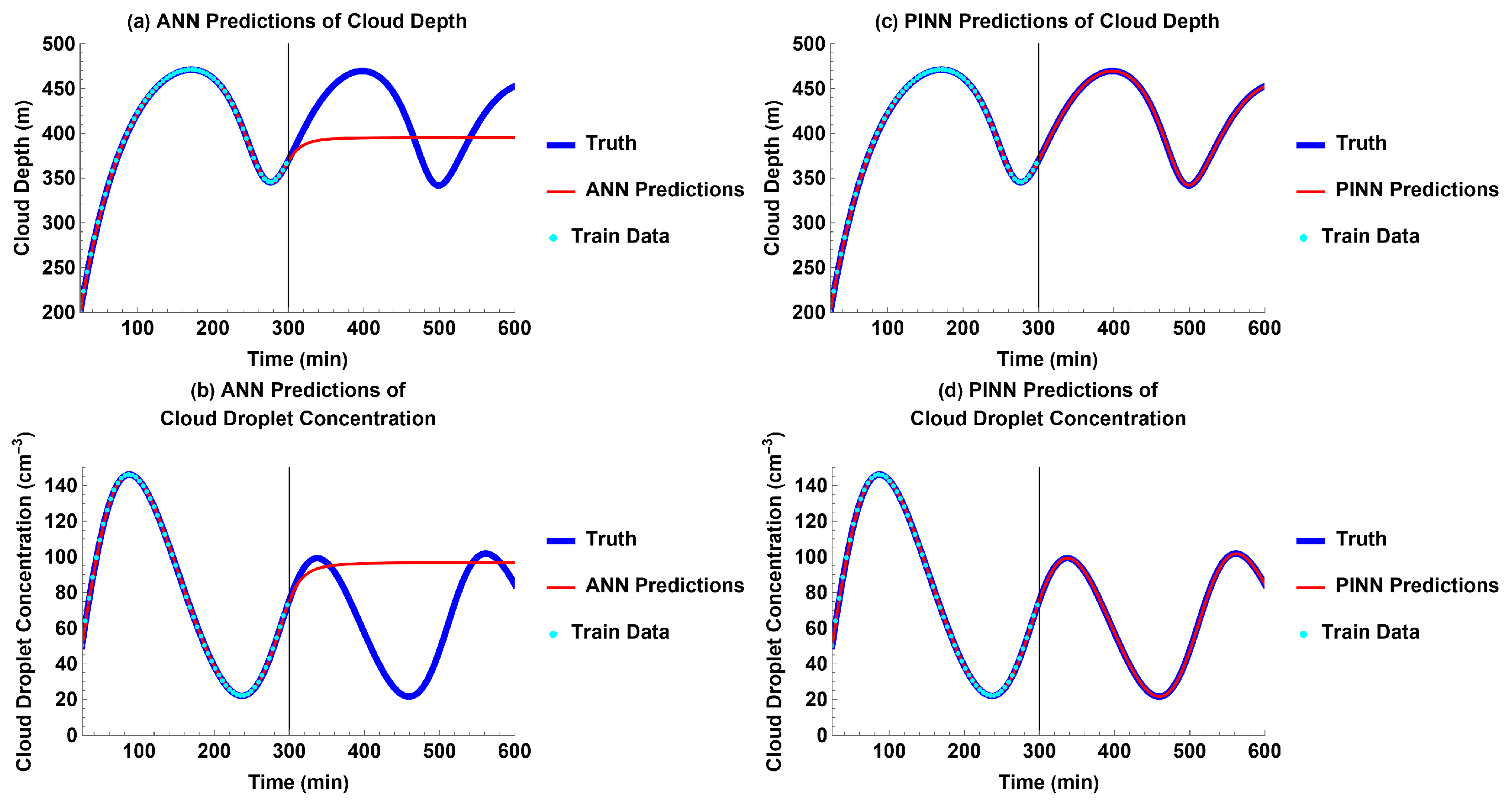
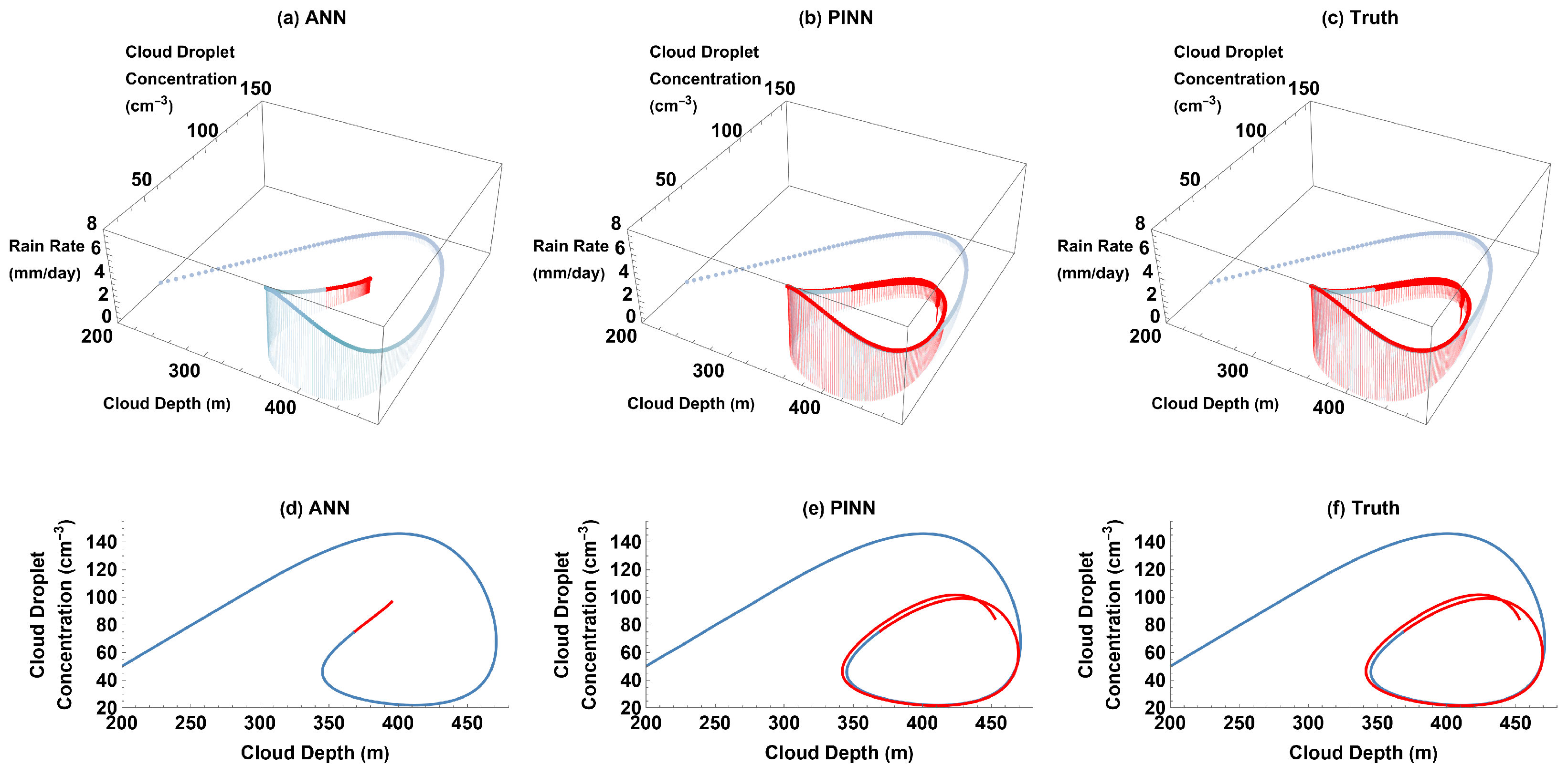
3.1.1. Predicting the Future

For the experiment without external forcing, both the cloud depth and cloud droplet concentration exhibited weakly dampened oscillations. Both the ANN and PINN were able to fit to the training data. However, the ANN was unable to successfully learn the Koren–Feingold model to make predictions of the future, given the training data. It predicts that the cloud depth and cloud droplet concentration would quickly reach a steady state instead of continuing to oscillate beyond the time domain of the training data (Figure 2a,b). In contrast, the PINN was able to very accurately predict the future of the aerosol–cloud–precipitation system, even in the time domain without the training data (Figure 2c,d).

The dampened oscillations of cloud depth, cloud droplet concentration, and precipitation in the truth and PINN predictions can be visualized through parametric plots (Figure 3b,c,e,f). Similar to Figure 2a,b, Figure 3a,d shows that the ANN predicts nearly constant values for the cloud depth, cloud droplet concentration, and precipitation after a certain time, so the parametric plots of future predictions (Figure 3a,d) do not evolve much over time. Thus, the ANN does not learn the damped oscillation aspect of the aerosol–cloud–precipitation system. Conversely, the PINN predictions (Figure 3b,e) are visually very close to the plots generated with the truth (Figure 3c,f): over time, both plots show that cloud depth and cloud droplet concentration continue to oscillate with decreasing amplitudes. Because our main purpose is to predict and/or reconstruct the time evolution of the Koren–Feingold model’s solutions in a small data regime, we chose to visualize our results through these time series and parametric plots.

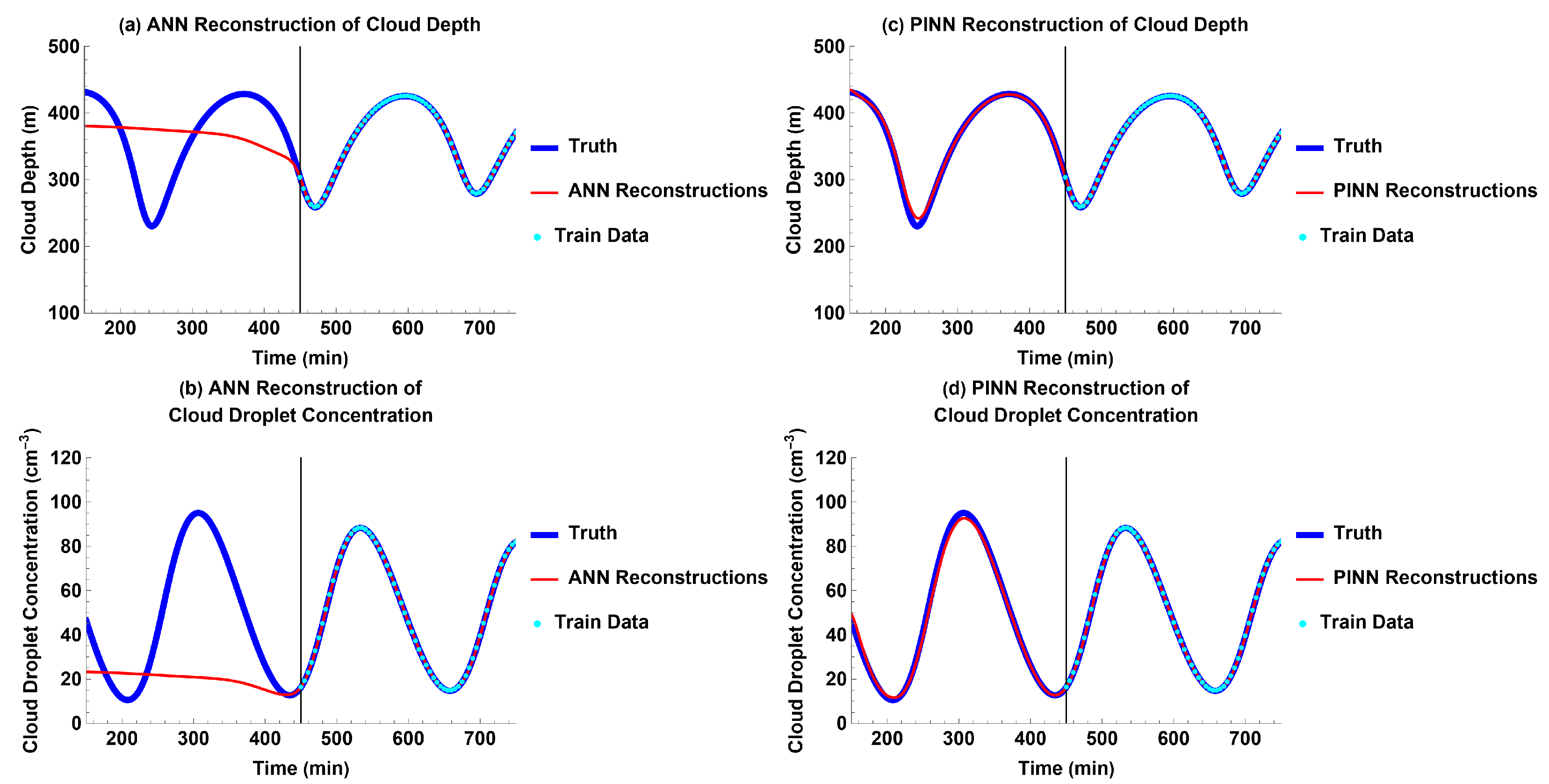
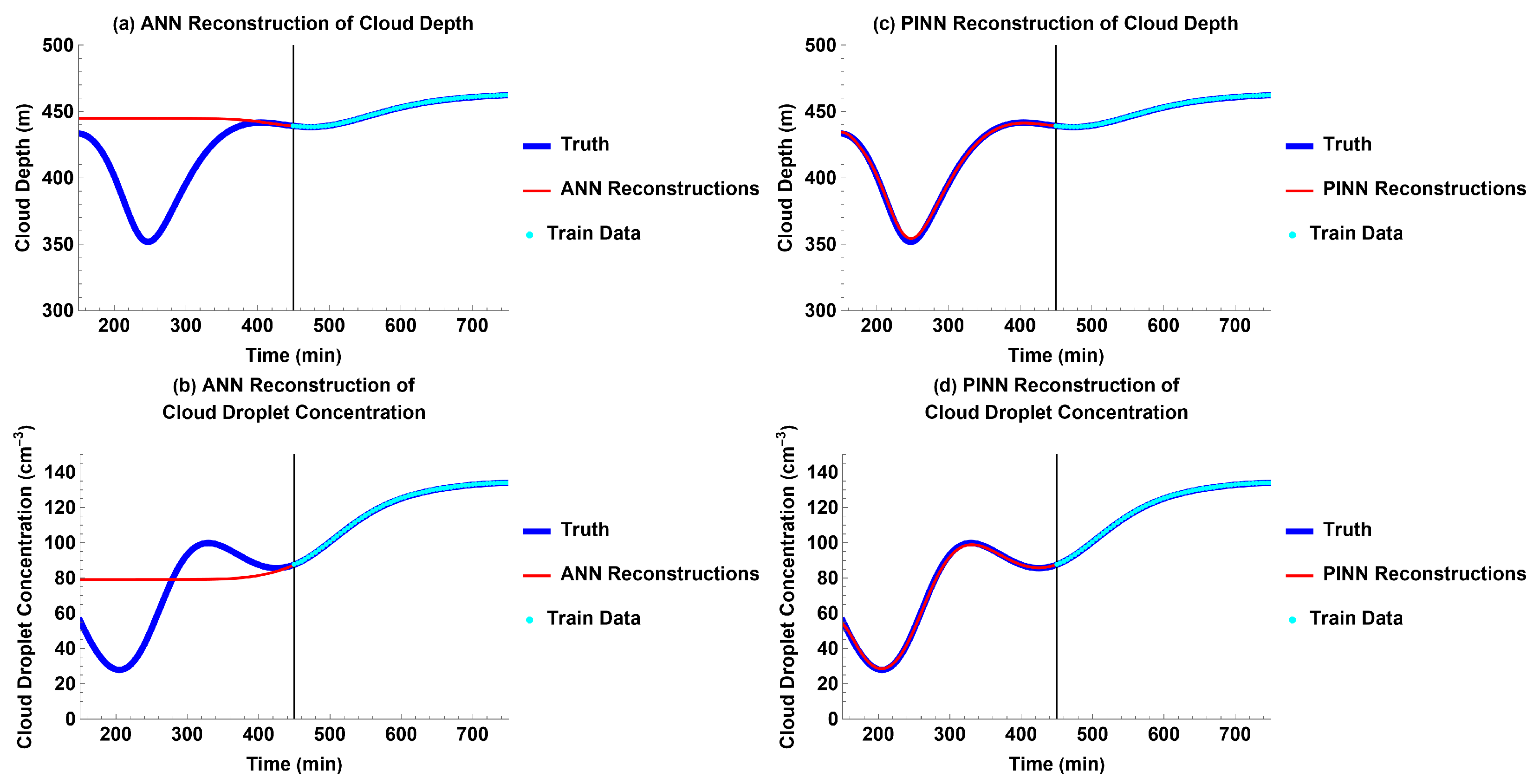
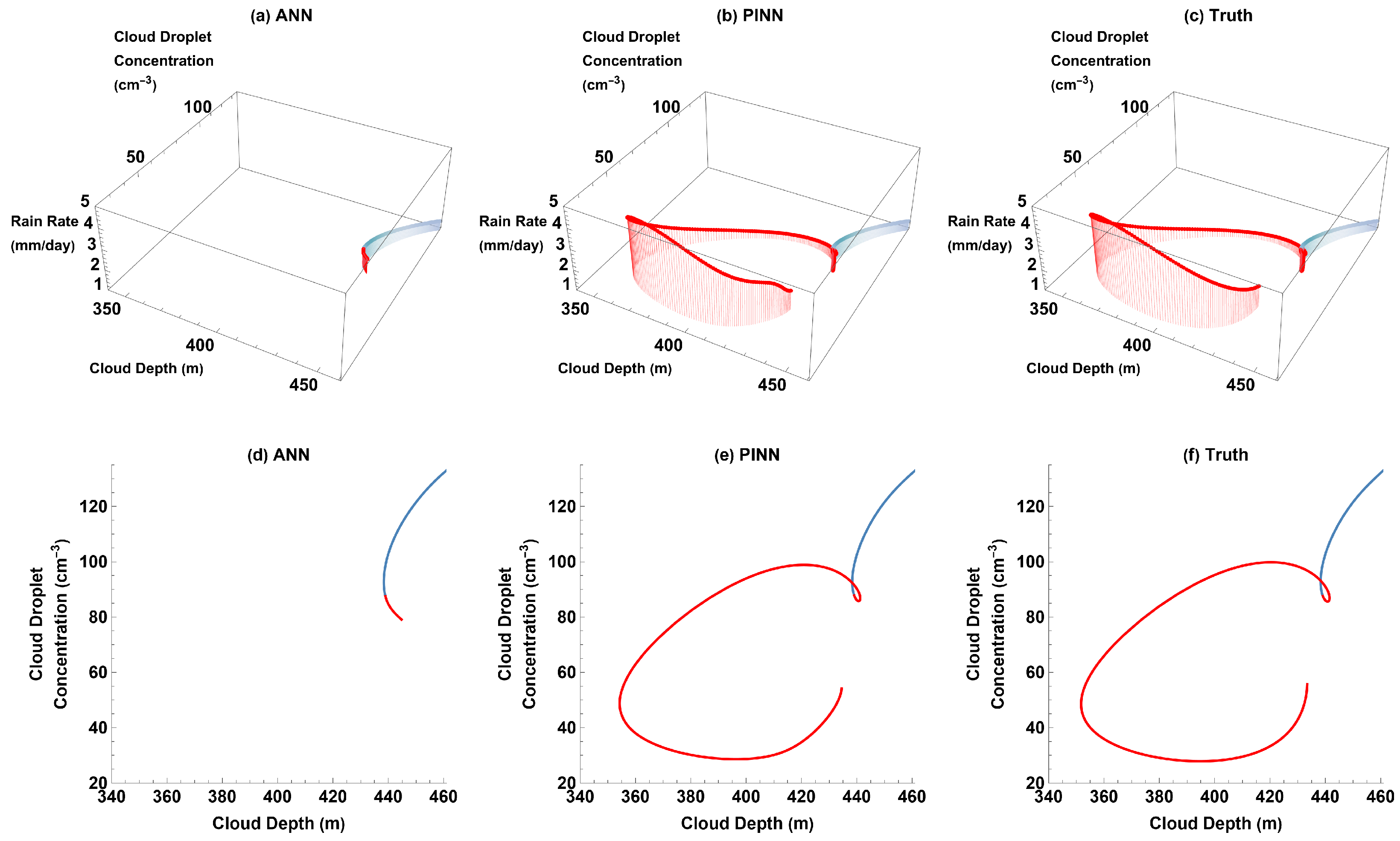
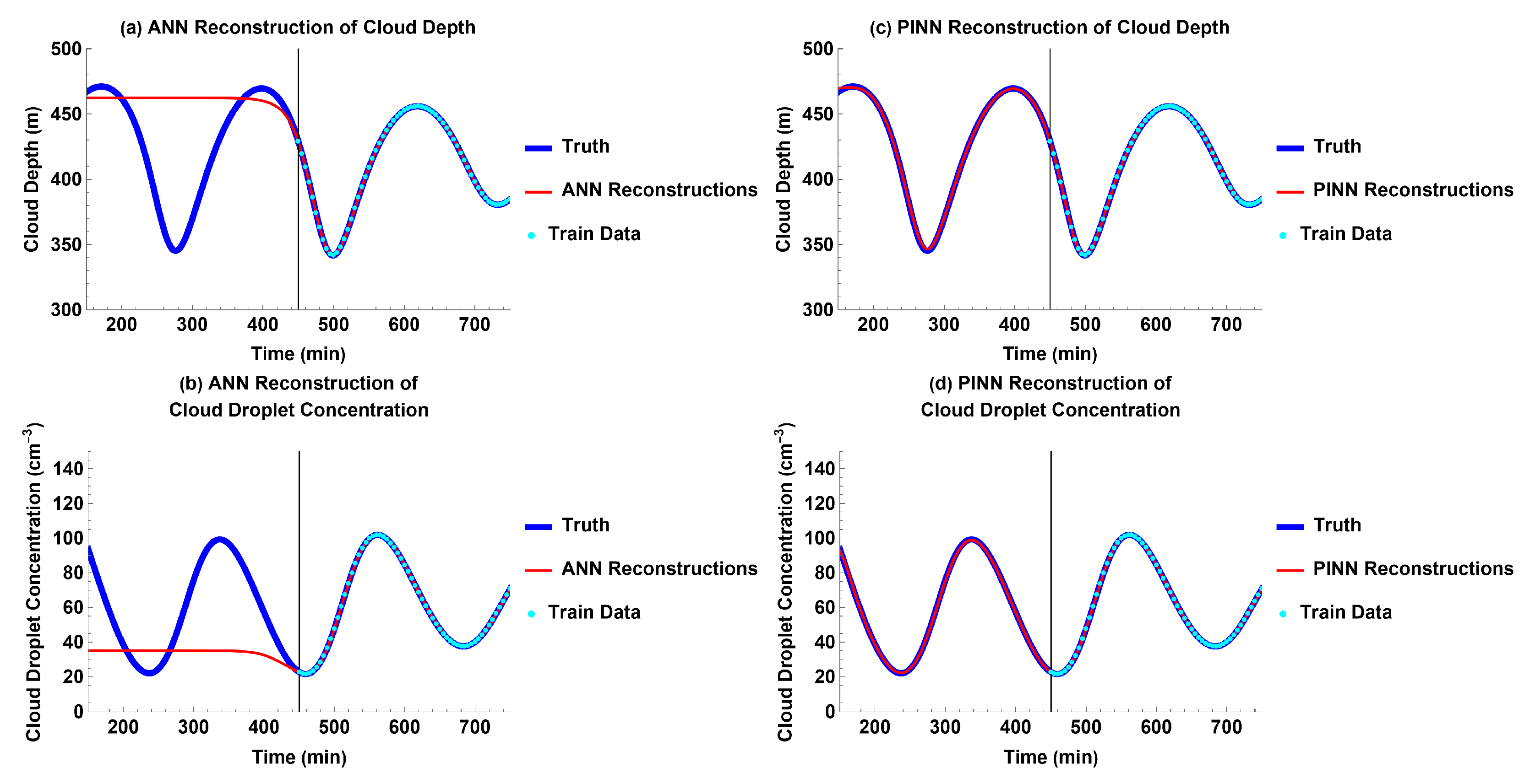
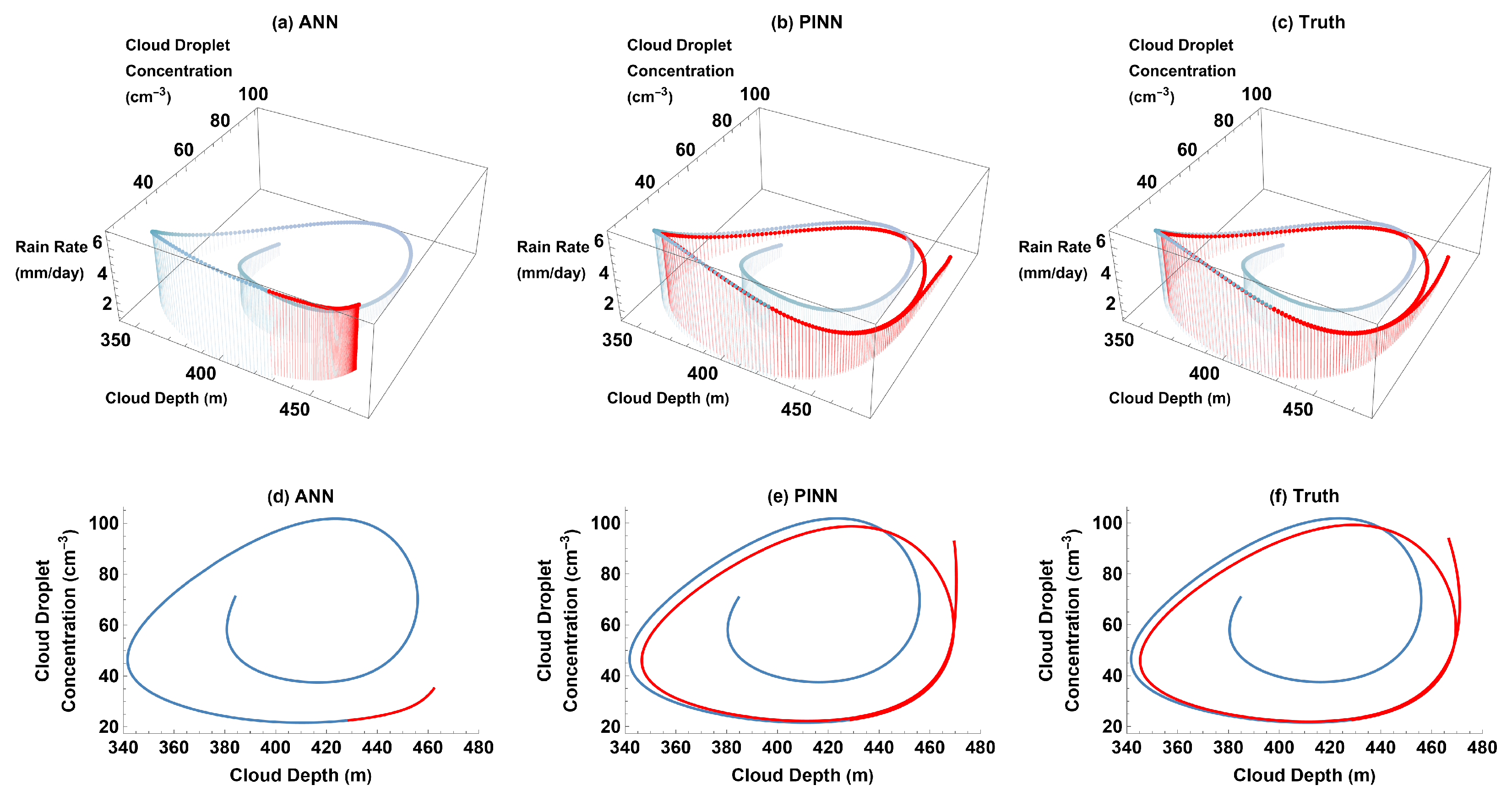
3.1.2. Reconstructing the Past

The time delay in the differential equations of the Koren–Feingold model makes the past reconstruction of cloud depth and cloud droplet concentration nontrivial. Similar to the experiment for future prediction without external forcing, the ANN is only able to fit to the training data and cannot reconstruct the past oscillations of cloud depth and cloud droplet concentration of the aerosol–cloud–precipitation system (Figure 4a,b and Figure 5a,d). However, even though the time delay makes the reconstruction of cloud depth and cloud droplet concentration challenging, the PINN is able to perform well in both future prediction and past reconstruction (Figure 2c,d and Figure 4c,d). It is able to reconstruct cloud depth and cloud droplet concentration for a past time domain equal in length to the time domain of the training data (Figure 4c,d).

In the parametric plots of the truth (Figure 5c,f), it is also evident that the oscillations of cloud depth and cloud droplet concentration decay in amplitude over time, so that the past has a larger amplitude than that of the training data given to the models. The reconstructions of the PINN also display the strengthened oscillations of the cloud depth and cloud droplet concentration in the reconstructed past, compared to the training data, and accurately reconstruct the aerosol–cloud–precipitation system’s past (Figure 5b,e).

We note that the main reason why it is possible to accurately reconstruct the past based on the Koren–Feingold model is that its equations do not have any diffusive/dissipative terms, and thus both the forward and the back-in-time models are well posed. In the presence of diffusion, however, reconstructing the past is notoriously ill-posed and only approximate (non-unique) solutions are possible [56,57,58,59,60]. Perhaps in a more general model than that of the Koren–Feingold, diffusive/dissipative processes may need to be accounted for; if so, recovering the past would not be as accurate and as easy as we demonstrate it to be for the Koren–Feingold model.

3.2. External Forcing Representing Increase in Aerosol Due to Wildfire

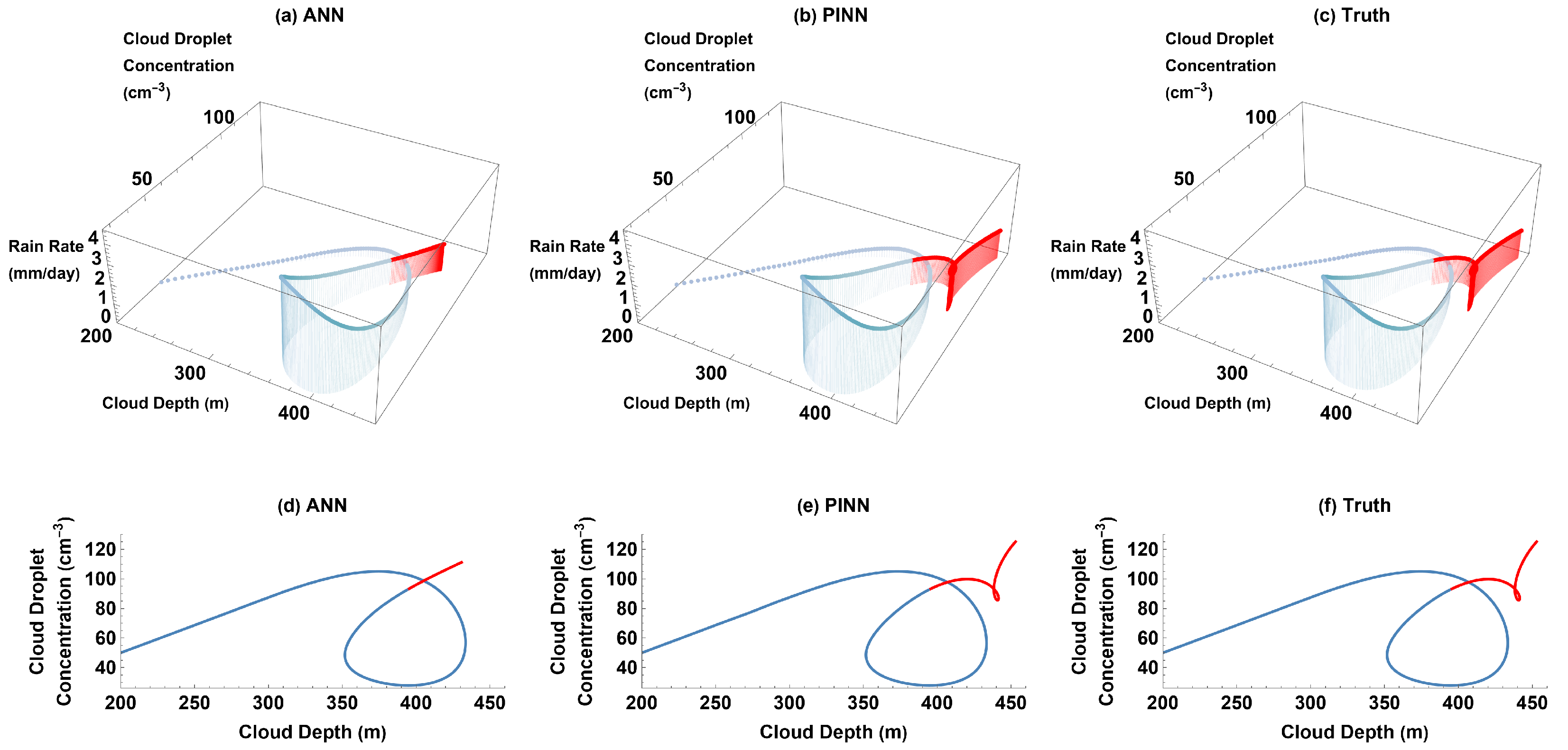
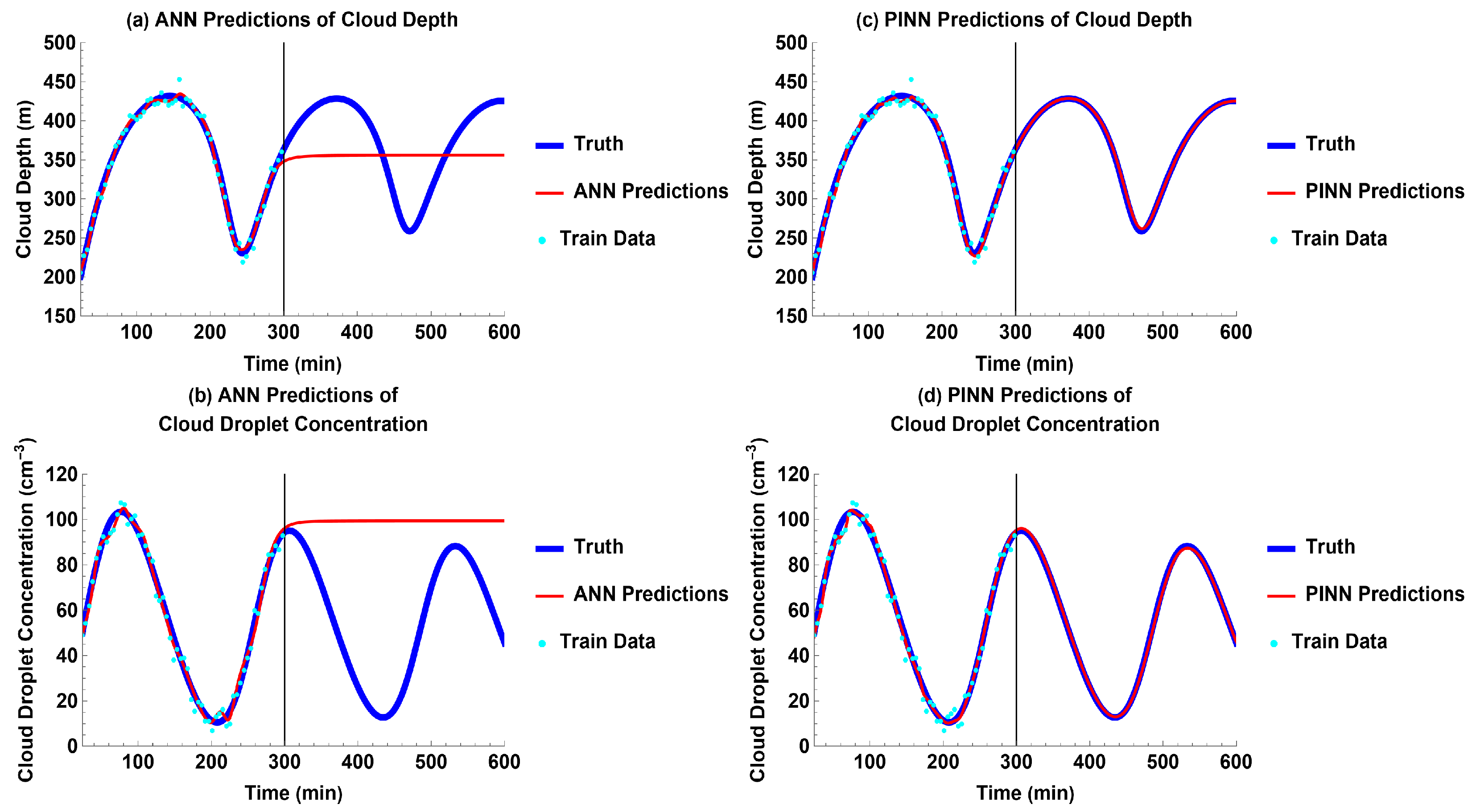
3.2.1. Predicting the Future

Compared to those without external forcing, adding external forcing to represent the sudden increase in aerosols due to wildfires (Equation (4)) results in significantly decayed oscillations for both cloud depth and cloud droplet concentration (Figure 2 and Figure 6). Due to the increase in the background aerosols, cloud droplet concentration eventually increases. Both cloud depth and cloud droplet concentration fluctuate very little as the oscillations become limited in amplitude over time (Figure 6 and Figure 7c,f). Similar to the experiments without external forcing, ANN predictions of cloud depth and cloud droplet concentration quickly reach a steady state after a certain time (Figure 2a,b, Figure 6a,b and Figure 7a,d). However, the PINN is able to further minimize its loss, successfully learn the Koren–Feingold model, and make predictions for cloud depth and cloud droplet concentration that are accurate to the truth (Figure 6c,d and Figure 7b,e). To learn the Koren–Feingold conceptual model with external forcing, such as an increase in environmental aerosols, the addition of physics loss to the total loss in the training process is crucial.

The introduction of external forcing representing the increase in wildfire-induced aerosols reduces precipitation compared to that produced by the unmodified Koren–Feingold model, as shown in the truth (Figure 5c and Figure 7c). The reduction in precipitation is consistent with the increase in cloud droplet concentration (Equation (3)). The PINN’s ability to replicate the impact of wildfire aerosols on precipitation (Figure 7b) proves that it is a viable way to study simple models of an aerosol–cloud–precipitation system.

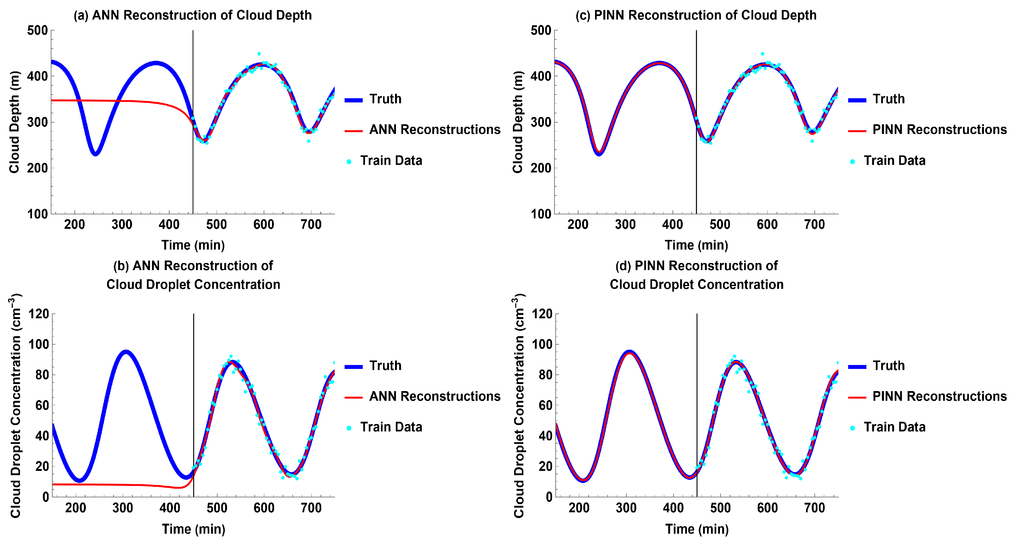
3.2.2. Reconstructing the Past

In addition to the time delay, the large difference in amplitude of the oscillations of cloud depth and cloud droplet concentration between the training time domain and the reconstructed time domain makes past reconstruction difficult (Figure 8). The data we used to train the models contain oscillations that are significantly weaker than the truth over the reconstruction time domain (Figure 9c,f), making reconstruction using the ANN (Figure 8a,b and Figure 9a,d) a challenging task without the addition of physics.

In this experiment, the PINN demonstrates its ability to accurately reconstruct a more complicated past while only training on limited data that were significantly dampened by the influx of wildfire aerosols (Figure 8c,d and Figure 9b,e).

Again, as we noted earlier, the main reason why it is possible to accurately reconstruct the past based on the Koren–Feingold model is that its equations do not have any diffusive/dissipative terms, and thus both the forward and the back-in-time models are well posed.

3.3. External Forcing Representing the Diurnal Cycle in Cloud Depth

For the experiment with external forcing representing the diurnal cycle in cloud depth, $N_{max}$ is increased from $180\mathrm{c}{\mathrm{m}}^{-3}$ to $250\mathrm{c}{\mathrm{m}}^{-3}$ to prevent cloud depth and cloud droplet concentration from becoming unstable when the background cloud depth $H_{max}$ becomes larger, as discussed by Koren and Feingold [1]. Since increasing background aerosol concentration serves to dampen the oscillations of cloud depth and cloud droplet concentration, the system rapidly reaches a steady state without adding the diurnal cycle of cloud depth. However, with the diurnal cycle of cloud depth (Equation (6)), the initial increase in the background cloud depth $H_{max}$ excites dampened oscillations in the aerosol–cloud–precipitation system at a shorter period than the diurnal cycle (Figure 10). Over a much longer time, however, the damped oscillations of the unmodified Koren–Feingold system decay. Thus, with the external forcing, the aerosol–cloud–precipitation system eventually becomes dominated by the oscillations of the diurnal cycle, and the system oscillates at a diurnal period.

3.3.1. Predicting the Future

The initial oscillations of cloud depth and cloud droplet concentration are much less uniform due to the diurnal cycle of clouds (Figure 11c,f). The PINN is able to accurately predict future cloud depth and cloud droplet concentration beyond the time domain of the training data (Figure 10c,d and Figure 11b,e), while the ANN is only able to learn the Koren–Feingold model during the time domain of the training data (Figure 10a,b and Figure 11a,d).

3.3.2. Reconstructing the Past

The past reconstructions of the ANN for cloud depth and cloud droplet concentration quickly reach a steady state (Figure 12a,b and Figure 13a,d). The PINN successfully reconstructs the past of an aerosol–cloud–precipitation system, including the diurnal cycle of clouds (Figure 12c,d and Figure 13b,e) with similar accuracy to future predictions for this system (Figure 10c,d and Figure 11b,e). Compared to the experiments for external forcing that increased the background aerosol concentration (Figure 9c,f), the difference between the amplitudes of oscillations of the training time domain and the reconstruction time domain for a system that includes the diurnal cycle of clouds is less dramatic (Figure 13c,f).

Again, it is possible to accurately reconstruct the past based on the Koren–Feingold model because its equations do not have any diffusive/dissipative terms, and thus both the forward and the back-in-time models are well posed.

3.4. Mean Squared Error Loss and Physics Mean Squared Error Loss for All Predictions and Reconstructions

Table 1. Mean squared error (MSE) of ANN and PINN over the prediction/reconstruction time domain for cloud depth and cloud droplet concentration for all experiments.

Experiment Name	Artificial Neural Network		Physics-Informed Neural Network
	$\mathbf{MSE}\mathbf{for}\mathbf{Cloud}\mathbf{Depth}\left({\mathbf{m}}^2\right)$	$\mathbf{MSE}\mathbf{for}\mathbf{Cloud}\mathbf{Droplet}\mathbf{Concentration}\left(\mathbf{c}{\mathbf{m}}^{-6}\right)$	$\mathbf{MSE}\mathbf{for}\mathbf{Cloud}\mathbf{Depth}\left({\mathbf{m}}^2\right)$	$\mathbf{MSE}\mathbf{for}\mathbf{Cloud}\mathbf{Droplet}\mathbf{Concentration}\left(\mathbf{c}{\mathbf{m}}^{-6}\right)$
Prediction	$4904.94$	$2674.28$	$0.18$	$0.025$
Reconstruction	$4269.27$	$1434.39$	$19.35$	$2.92$
Prediction with wildfire	$151.49$	$219.40$	$0.00062$	$0.0014$
Reconstruction with wildfire	$2106.81$	$719.56$	$1.22$	$0.58$
Prediction with the diurnal cycle	$2176.28$	$1520.33$	$0.075$	$0.026$
Reconstruction with the diurnal cycle	$2631.32$	$1235.47$	$0.57$	$0.18$

lists the mean squared error (MSE) loss for ANN and PINN for the prediction and reconstruction time domains, respectively, with the truth serving as the ‘test’ set (see Methods Section 2.6). The mean squared error losses of the predictions and reconstructions of the ANN are much larger than those of the predictions and reconstructions of the PINN (Table 1), highlighting the great improvement that the addition of physics makes to the accuracy of prediction and reconstruction of the aerosol–cloud–precipitation system and the learning of the Koren–Feingold model.

Table 2. Physics mean squared error (MSE) loss of PINN over the prediction/reconstruction time period (on the predicted and reconstructed physics time domain) for cloud depth and cloud droplet concentration for all experiments.

Experiment Name	$\mathit{M}\mathit{S}{\mathit{E}}_{\mathit{p}\mathit{h}\mathit{y}\mathit{s}\mathit{i}\mathit{c}\mathit{s}}^{\mathit{H}}$$\mathbf{for}\mathbf{Cloud}\mathbf{Depth}({\mathbf{m}}^2/{\mathbf{m}\mathbf{i}\mathbf{n}}^2)$	$\mathit{M}\mathit{S}{\mathit{E}}_{\mathit{p}\mathit{h}\mathit{y}\mathit{s}\mathit{i}\mathit{c}\mathit{s}}^{\mathit{N}}$$\mathbf{for}\mathbf{Cloud}\mathbf{Droplet}\mathbf{Concentration}(\mathbf{c}{\mathbf{m}}^{-6}/{\mathbf{m}\mathbf{i}\mathbf{n}}^2)$
Prediction	$0.049\times {10}^{-4}$	$0.074\times {10}^{-4}$
Reconstruction	$0.22\times {10}^{-4}$	$0.37\times {10}^{-4}$
Prediction with wildfire	$0.016\times {10}^{-4}$	$0.019\times {10}^{-4}$
Reconstruction with wildfire	$0.0090\times {10}^{-4}$	$0.016\times {10}^{-4}$
Prediction with the diurnal cycle	$0.27\times {10}^{-4}$	$0.16\times {10}^{-4}$
Reconstruction with the diurnal cycle	$0.075\times {10}^{-4}$	$0.064\times {10}^{-4}$

lists the PINN’s physics mean squared error loss for the prediction and reconstruction time domains, respectively (see Methods Section 2.6). The physics mean squared error losses for both future prediction and past reconstruction are very small (Table 2), justifying the use of the regularization factor $\lambda ={10}^4$ in the training process. The very small physics MSE losses are consistent with the fact that the PINN is able to accurately predict the future and reconstruct the past of the aerosol–cloud–precipitation system, despite challenges such as the time delay in the differential equations and the decay of oscillations of cloud depth and cloud droplet concentration.

3.5. Sensitivity of PINN to the Regularization Factor of Physics Loss

The sensitivity of the PINN to the regularization factor $\lambda$ of physics loss was tested for different values of $\lambda$. Figure 14 shows that, for the past reconstruction without external forcing, values of $\lambda$ that are too small or too large prevent the PINN from accurately reconstructing the past. If $\lambda$ is too small ($\lambda =1\times {10}^2$), the data loss dominates and the PINN does not fit well to the physical equations (Figure 14a,f). If $\lambda$ is too large ($\lambda =1\times {10}^6$), the physics loss dominates and the PINN does not fit well to the training data (Figure 14e,j). For the intermediate values of $\lambda =1\times {10}^3$, $\lambda =1\times {10}^4$, and $\lambda =1\times {10}^5$, the PINN’s accuracy is not very sensitive to the value of $\lambda$, and there is very little difference between the past reconstructions (Figure 14b–d,g–i). Thus, the choice of $\lambda =1\times {10}^4$ that we use in this paper is reasonable. These results demonstrate that it is important for the PINN to include both data and physics. Without one or the other, the PINN does not perform as well.

3.6. Sensitivity of ANN and PINN to Random Noise Added to the Training Data

To test how the ANNs and PINNs perform when trained on data biased by measurement errors, we added random Gaussian noise to the training data. Two additional experiments were conducted with noisy training data for future prediction and past reconstruction without external forcing. Random Gaussian noises with standard deviations of $8\mathrm{m}$ for cloud depth and $4\mathrm{c}{\mathrm{m}}^{-3}$ for cloud droplet concentration were, respectively, added to the training data. The standard deviations of these noises were about 11% (for cloud depth) and 13% (for cloud droplet concentration) of the standard deviations of the original, noiseless training data for the future prediction, and about 14% (for cloud depth) and 16% (for cloud droplet concentration) of the standard deviations of the original, noiseless training data for the past reconstruction. For these experiments, the ANN was trained simultaneously with both a training dataset and a validation dataset to avoid overfitting to the noise in the training data. The validation dataset was separately created by adding random Gaussian noise with the same standard deviations as listed above to the same original, noiseless training data.

In both experiments with noisy training data, the PINN still outperformed the ANN in the future prediction and the past reconstruction of aerosol–cloud–precipitation interactions, and it was able to learn the Koren–Feingold conceptual model despite the noise included in the training data (Figure 15 and Figure 16). On the other hand, the ANN was still unable to extrapolate over the prediction/reconstruction domains (Figure 15 and Figure 16).

4. Discussion

With the addition of external forcing in the form of wildfire-induced aerosols to the maximum cloud droplet concentration as a function of time, the predictions and reconstructions of the physics-informed neural network (PINN) show that rainfall is suppressed as aerosol increases. This creates a positive feedback loop, as minimal precipitation creates a drier environment conducive to wildfires. As wildfires continue to release smoke aerosols into the atmosphere, precipitation that could help stop the wildfire and its release of smoke aerosols into the atmosphere is further suppressed. Thus, an increase in wildfire-induced aerosols is likely to result in further wildfires [61]. We find that adding a sudden increase in wildfire-induced aerosols, and thereby increasing the background cloud droplet concentration, heavily dampens the normal oscillatory behavior of the system that occurs without any external forcing. We also find that the initial increase in the background cloud depth can excite damped oscillation in the aerosol–cloud–precipitation system at a shorter period than that of the diurnal cycle.

The PINN successfully predicts and reconstructs the aerosol–cloud–precipitation interactions of the original Koren–Feingold model. PINNs are also able to predict and reconstruct aerosol–cloud–precipitation interactions with the effects of external forcing such as wildfires or the diurnal cycle of clouds on the aerosol–cloud–precipitation system. As shown in Section 3.5, the accuracy of the PINN is not sensitive to the value of the regularization factor ($\lambda$), a key parameter for the PINN that controls the weight for the physics loss relative to the data loss, for a broad range (from $\lambda =1\times {10}^3$ to $\lambda =1\times {10}^5$). Thus, our choice of $\lambda =1\times {10}^4$ used in this paper is reasonable.

Our study shows that PINNs significantly outperform ANNs in both future predictions and past reconstructions. The main reason for ANN’s poor performance with small (narrow) training datasets is the fact that, as opposed to PINNs, they are not informed by the laws of physics. As discussed in the Introduction section, many pure data-driven machine learning techniques have been successful in predictions because of the large ratio between the total time interval of the training data and the prediction time interval, often on the order of more than 100:1 [27,31,33]. On the other hand, our study focuses on a small data regime with limited training data, where the ratio between the total time interval of the training data and the prediction/reconstruction time interval is close to 1:1. ANN’s poor performance is also related to its inability to extrapolate outside of the given training data.

We conducted an additional future prediction simulation using the ANN by expanding the training data from an original time interval of 276 min to 561 min and reducing the prediction time interval from 300 min to 15 min. Thus, the ratio between the total time interval of the training data and the prediction time interval increases from about 0.9:1 to about 37:1. In this new simulation, the ANN performs well in both the expanded training data interpolation domain and the reduced prediction extrapolation domain. For the new prediction domain, the MSE loss (evaluated every minute) is 20.45 for cloud depth (${\mathrm{m}}^2$) and 11.38 for cloud droplet concentration (${\mathrm{c}\mathrm{m}}^{-6}$), respectively, much smaller than that for the original prediction domain (evaluated every 10 min) using the ANN: 4904.94 for cloud depth (${\mathrm{m}}^2$) and 2674.28 for cloud droplet concentration (${\mathrm{c}\mathrm{m}}^{-6}$), respectively. We also conducted an additional past reconstruction simulation using the ANN by expanding the training data from an original time interval of 300 min to 585 min and reducing the reconstruction time interval from 300 min to 15 min. Thus, the ratio between the total time interval of the training data and the reconstruction time interval increased from about 1:1 to about 39:1. In this new simulation, the ANN performed well in both the expanded training data interpolation domain and the reduced reconstruction extrapolation domain. For the new reconstruction domain, the MSE loss (evaluated every minute) was 0.031 for cloud depth (${\mathrm{m}}^2$) and 7.76 for cloud droplet concentration (${\mathrm{c}\mathrm{m}}^{-6}$), respectively, much smaller than that for the original reconstruction domain (evaluated every 10 min) using the ANN: 4296.29 for cloud depth (${\mathrm{m}}^2$) and 1434.39 for cloud droplet concentration (${\mathrm{c}\mathrm{m}}^{-6}$), respectively. These new simulations support our explanation that the ANN’s poor performance is partially due to the small ratio between the total time interval of the training data and the prediction/reconstruction time interval; ANNs thus act as smart interpolators within the range of the training dataset, but they cannot extrapolate far outside this range, a typical characteristic of interpolation functions. It is unsurprising that the ANN performs well in both the expanded training data interpolation domain and the reduced prediction extrapolation domain that is close to the interpolation domain.

Our PINNs, on the other hand, being trained on the same small dataset, are additionally informed by the physics of the Koren–Feingold model. Thus, it is not surprising that they do well in the predictive mode. Since, as we point out in the paper, the Koren–Feingold model has no diffusive terms, it is also not surprising that the PINNs do well in the reconstructive modes. Another reason why the ANNs failed in future predictions and past reconstructions was the small size of our training dataset. Indeed, previous studies find the performance of ANNs to be excellent with large training datasets, but its quality deteriorates with the decreasing size of the training datasets [35]. Finally, the time-varying external forcings over the prediction and reconstruction time domains cannot be successfully learned by ANNs over the small time interval of the training time domain. The PINN is able to incorporate the knowledge of the time-varying external forcings. Thus, it has an important advantage over ANNs when predicting and reconstructing aerosol–cloud–precipitation interactions from the Koren–Feingold model with added time-varying external forcings.

As already mentioned, the main reason why it is possible to accurately reconstruct the past based on the Koren–Feingold model is that its equations do not have any diffusive/dissipative terms, and thus both the forward and the back-in-time models are well posed. In the presence of diffusion, however, reconstructing the past is notoriously ill-posed, and only approximate (non-unique) solutions are possible [56,57,58,59,60]. Perhaps in a more general model than that of the Koren–Feingold, diffusive/dissipative processes may need to be accounted for; if so, recovering the past would not be as accurate and as easy as we demonstrate it to be for the Koren–Feingold model.

5. Conclusions

We studied a Koren–Feingold model of an aerosol–cloud–precipitation system with neural networks, i.e., the physics-informed neural network (PINN), and investigated the PINN’s ability to learn the Koren–Feingold model. This study is the first to use PINNs to predict the Koren–Feingold model and reconstruct the past of an aerosol–cloud–precipitation system in a small data regime. Another novel aspect is the modification of the differential equations of the Koren–Feingold model to include external forcings, such as wildfire-induced aerosols or the diurnal cycle of clouds, investigating for the first time the respective impacts of including externally forced aerosols or the diurnal cycle of cloud depth on the conceptual Koren–Feingold model. We show for the first time that PINNs are able to perform well when external forcings are added to the conceptual Koren–Feingold model.

Our study demonstrates that PINNs greatly improve upon the traditional ANN’s ability to learn the Koren–Feingold model, predict the future, and reconstruct the past of the aerosol–cloud–precipitation system. We show that the combination of a simple ANN and a physical model produces a PINN model that is much more accurate in predictive and reconstructive modes, even for a small training dataset. The ANN is able to learn the conceptual Koren–Feingold model during the training time interval but is unable to accurately predict cloud depth and cloud droplet concentration over the time domain once outside the training time interval. The PINN successfully predicts the future and reconstructs the past through learning the original differential equations of the Koren–Feingold model, significantly outperforming the ANN. The PINN also learns the modified Koren–Feingold model that separately introduces wildfire-induced aerosols and the diurnal cloud cycle. The PINN is able to achieve visually similar results to the truth throughout both the training domain and the prediction/reconstruction domains in this study, proving that it successfully learned the Koren–Feingold model.

Many previous studies focused on using PINNs to predict the future of dynamic systems [35,45,46]. The PINN’s ability to reconstruct the past with limited data for a dynamic system with nonlinear delayed differential equations such as the Koren–Feingold model is underexplored. Here, we show that the PINN performs similarly well for past reconstruction compared to future prediction, despite the time delay feature of the differential equations of the Koren–Feingold model, which makes the past reconstruction nontrivial. When the solution of the Koren–Feingold model exhibits heavily dampened oscillations, the truth data that are used to train the models contain oscillations that are much weaker than those in the past time domain, making the past reconstruction a challenging task. The addition of physics loss to the PINN that differentiates it from the ANN is especially beneficial for the task of reconstructing the past (as long as there are no diffusive/dissipative terms in the underlying model). We demonstrate that when informed by the Koren–Feingold model, PINNs with a small training dataset are able not only to predict the future, as some researchers have already shown, e.g., [35,45,46], but also reconstruct the past, which we do here for the first time. We recommend that PINNs be used to predict and reconstruct solutions of delayed differential equations similar to those of the Koren–Feingold model in a small data regime.

For the majority of experiments conducted in our study, the training dataset was generated by solving the delayed differential equations of the Koren–Feingold model of aerosol–cloud–precipitation interactions (using Mathematica’s NDSolve super-function), rather than from physical observations. Thus, there is no noise present in the training dataset that would necessitate the use of decomposition methods to capture this noise. We also included two additional experiments with random noise added to the original, noiseless training dataset, and show that the PINN still outperforms the ANN in the future prediction and the past reconstruction of aerosol–cloud–precipitation interactions, despite the noise included in the training data.

One way to build on the results of this study would be to solve the differential equations of the Koren–Feingold model over successive time domains and train the PINN with its predictions of the system [62]. This strategy would improve PINN accuracy when studying complex systems and equations.

References

1. Koren, I.; Feingold, G. Aerosol-cloud-precipitation system as a predator-prey problem. Proc. Natl. Acad. Sci. USA 2011, 108, 12227–12232. [Google Scholar] [CrossRef] [PubMed]
2. Fu, H.; Lin, Y. A kinematic model for understanding rain formation efficiency of a convective cell. J. Adv. Model. Earth Syst. 2019, 11, 4395–4422. [Google Scholar] [CrossRef]
3. Pujol, O.; Jensen, A. Cloud–rain predator–prey interactions: Analyzing some properties of the Koren–Feingold model and introduction of a new species-competition bulk system with a Hopf bifurcation. Phys. D Nonlinear Phenom. 2019, 399, 86–94. [Google Scholar] [CrossRef]
4. Mülmenstädt, J.; Feingold, G. The radiative forcing of aerosol–cloud interactions in liquid clouds: Wrestling and embracing uncertainty. Curr. Clim. Chang. Rep. 2018, 4, 23–40. [Google Scholar] [CrossRef]
5. Goren, T.; Feingold, G.; Gryspeerdt, E.; Kazil, J.; Kretzschmar, J.; Jia, H.; Quaas, J. Projecting stratocumulus transitions on the albedo—Cloud fraction relationship reveals linearity of albedo to droplet concentrations. Geophys. Res. Lett. 2022, 49, e2022GL101169. [Google Scholar] [CrossRef]
6. Twomey, S. The influence of pollution on the shortwave albedo of clouds. J. Atmos. Sci. 1977, 34, 1149–1152. [Google Scholar] [CrossRef]
7. Berhane, S.A.; Bu, L. Aerosol—Cloud interaction with summer precipitation over major cities in Eritrea. Remote Sens. 2021, 13, 677. [Google Scholar] [CrossRef]
8. Lunderman, S.; Morzfeld, M.; Glassmeier, F.; Feingold, G. Estimating parameters of the nonlinear cloud and rain equation from a large-eddy simulation. Phys. D Nonlinear Phenom. 2020, 410, 132500. [Google Scholar] [CrossRef]
9. Barnaba, F.; Angelini, F.; Curci, G.; Gobbi, G.P. An important fingerprint of wildfires on the European aerosol load. Atmos. Chem. Phys. 2011, 11, 10487–10501. [Google Scholar] [CrossRef]
10. Hallar, A.G.; Molotch, N.P.; Hand, J.L.; Livneh, B.; McCubbin, I.B.; Petersen, R.; Kunkel, K.E. Impacts of increasing aridity and wildfires on aerosol loading in the intermountain Western US. Environ. Res. Lett. 2017, 12, 014006. [Google Scholar] [CrossRef]
11. Jahl, L.G.; Brubaker, T.A.; Polen, M.J.; Jahn, L.G.; Cain, K.P.; Bowers, B.B.; Sullivan, R.C. Atmospheric aging enhances the ice nucleation ability of biomass-burning aerosol. Sci. Adv. 2021, 7, eabd3440. [Google Scholar] [CrossRef] [PubMed]
12. Battula, S.B.; Siems, S.; Mondal, A.; Ghosh, S. Aerosol-heavy precipitation relationship within monsoonal regimes in the Western Himalayas. Atmos. Res. 2023, 288, 106728. [Google Scholar] [CrossRef]
13. Liu, J.; Zhu, Y.; Wang, M.; Rosenfeld, D.; Cao, Y. Marine warm cloud fraction decreases monotonically with rain rate for fixed vertical and horizontal cloud sizes. Geophys. Res. Lett. 2023, 50, e2022GL101680. [Google Scholar] [CrossRef]
14. Sharma, P.; Ganguly, D.; Sharma, A.K.; Kant, S.; Mishra, S. Assessing the aerosols, clouds and their relationship over the northern Bay of Bengal using a global climate model. Earth Space Sci. 2023, 10, e2022EA002706. [Google Scholar] [CrossRef]
15. Lee, H.; Jeong, S.J.; Kalashnikova, O.; Tosca, M.; Kim, S.W.; Kug, J.S. Characterization of wildfire-induced aerosol emissions from the Maritime Continent peatland and Central African dry savannah with MISR and CALIPSO aerosol products. J. Geophys. Res. Atmos. 2018, 123, 3116–3125. [Google Scholar] [CrossRef]
16. Rozendaal, M.A.; Leovy, C.B.; Klein, S.A. An observational study of diurnal variations of marine stratiform cloud. J. Clim. 1995, 8, 1795–1809. [Google Scholar] [CrossRef]
17. Wood, R.; Bretherton, C.S.; Hartmann, D.L. Diurnal cycle of liquid water path over the subtropical and tropical oceans. Geophys. Res. Lett. 2002, 29, 7-1–7-4. [Google Scholar] [CrossRef]
18. Min, M.; Zhang, Z. On the influence of cloud fraction diurnal cycle and sub-grid cloud optical thickness variability on all-sky direct aerosol radiative forcing. J. Quant. Spectrosc. Radiat. Transf. 2014, 142, 25–36. [Google Scholar] [CrossRef]
19. Chepfer, H.; Brogniez, H.; Noël, V. Diurnal variations of cloud and relative humidity profiles across the tropics. Sci. Rep. 2019, 9, 16045. [Google Scholar] [CrossRef]
20. Noel, V.; Chepfer, H.; Chiriaco, M.; Yorks, J. The diurnal cycle of cloud profiles over land and ocean between 51 S and 51 N, seen by the CATS spaceborne lidar from the International Space Station. Atmos. Chem. Phys. 2018, 18, 9457–9473. [Google Scholar] [CrossRef]
21. Wallace, J.M. Diurnal variations in precipitation and thunderstorm frequency over the conterminous United States. Mon. Weather Rev. 1975, 103, 406–419. [Google Scholar] [CrossRef]
22. Stubenrauch, C.J.; Chédin, A.; Rädel, G.; Scott, N.A.; Serrar, S. Cloud properties and their seasonal and diurnal variability from TOVS Path-B. J. Clim. 2006, 19, 5531–5553. [Google Scholar] [CrossRef]
23. LeCun, Y.; Bengio, Y.; Hinton, G. Deep learning. Nature 2015, 521, 436–444. [Google Scholar] [CrossRef] [PubMed]
24. Lagaris, I.E.; Likas, A.; Fotiadis, D.I. Artificial neural networks for solving ordinary and partial differential equations. IEEE Trans. Neural Netw. 1998, 9, 987–1000. [Google Scholar] [CrossRef] [PubMed]
25. Wilby, R.L.; Wigley, T.M.L.; Conway, D.; Jones, P.D.; Hewitson, B.C.; Main, J.; Wilks, D.S. Statistical downscaling of general circulation model output: A comparison of methods. Water Resour. Res. 1998, 34, 2995–3008. [Google Scholar] [CrossRef]
26. Lary, D.J.; Alavi, A.H.; Gandomi, A.H.; Walker, A.L. Machine learning in geosciences and remote sensing. Geosci. Front. 2016, 7, 3–10. [Google Scholar] [CrossRef]
27. Yuan, X.; Chen, C.; Lei, X.; Yuan, Y.; Muhammad Adnan, R. Monthly runoff forecasting based on LSTM–ALO model. Stoch. Environ. Res. Risk Assess. 2018, 32, 2199–2212. [Google Scholar] [CrossRef]
28. Ikram, R.M.A.; Mostafa, R.R.; Chen, Z.; Parmar, K.S.; Kisi, O.; Zounemat-Kermani, M. Water temperature prediction using improved deep learning methods through reptile search algorithm and weighted mean of vectors optimizer. J. Mar. Sci. Eng. 2023, 11, 259. [Google Scholar] [CrossRef]
29. Mostafa, R.R.; Kisi, O.; Adnan, R.M.; Sadeghifar, T.; Kuriqi, A. Modeling potential evapotranspiration by improved machine learning methods using limited climatic data. Water 2023, 15, 486. [Google Scholar] [CrossRef]
30. Adnan, R.M.; Mostafa, R.R.; Islam, A.R.M.T.; Kisi, O.; Kuriqi, A.; Heddam, S. Estimating reference evapotranspiration using hybrid adaptive fuzzy inferencing coupled with heuristic algorithms. Comput. Electron. Agric. 2021, 191, 106541. [Google Scholar] [CrossRef]
31. Adnan, R.M.; Dai, H.L.; Mostafa, R.R.; Parmar, K.S.; Heddam, S.; Kisi, O. Modeling multistep ahead dissolved oxygen concentration using improved support vector machines by a hybrid metaheuristic algorithm. Sustainability 2022, 14, 3470. [Google Scholar] [CrossRef]
32. Adnan, R.M.; Dai, H.L.; Mostafa, R.R.; Islam, A.R.M.T.; Kisi, O.; Heddam, S.; Zounemat-Kermani, M. Modelling groundwater level fluctuations by ELM merged advanced metaheuristic algorithms using hydroclimatic data. Geocarto Int. 2023, 38, 2158951. [Google Scholar] [CrossRef]
33. Adnan, R.M.; Meshram, S.G.; Mostafa, R.R.; Islam, A.R.M.T.; Abba, S.I.; Andorful, F.; Chen, Z. Application of Advanced Optimized Soft Computing Models for Atmospheric Variable Forecasting. Mathematics 2023, 11, 1213. [Google Scholar] [CrossRef]
34. Adnan, R.M.; Mostafa, R.R.; Dai, H.L.; Heddam, S.; Kuriqi, A.; Kisi, O. Pan evaporation estimation by relevance vector machine tuned with new metaheuristic algorithms using limited climatic data. Eng. Appl. Comput. Fluid Mech. 2023, 17, 2192258. [Google Scholar] [CrossRef]
35. Raissi, M.; Perdikaris, P.; Karniadakis, G.E. Physics-informed neural networks: A deep learning framework for solving forward and inverse problems involving nonlinear partial differential equations. J. Comput. Phys. 2019, 378, 686–707. [Google Scholar] [CrossRef]
36. Karniadakis, G.E.; Kevrekidis, I.G.; Lu, L.; Perdikaris, P.; Wang, S.; Yang, L. Physics-informed machine learning. Nat. Rev. Phys. 2021, 3, 422–440. [Google Scholar] [CrossRef]
37. Li, S.; Feng, X. Dynamic Weight Strategy of Physics-Informed Neural Networks for the 2D Navier–Stokes Equations. Entropy 2022, 24, 1254. [Google Scholar] [CrossRef]
38. Huang, Y.; Zhang, Z.; Zhang, X. A direct-forcing immersed boundary method for incompressible flows based on physics-informed neural network. Fluids 2022, 7, 56. [Google Scholar] [CrossRef]
39. Zhou, H.; Pu, J.; Chen, Y. Data-driven forward–inverse problems for the variable coefficients Hirota equation using deep learning method. Nonlinear Dyn. 2023, 111, 14667–14693. [Google Scholar] [CrossRef]
40. Omar, S.I.; Keasar, C.; Ben-Sasson, A.J.; Haber, E. Protein Design Using Physics Informed Neural Networks. Biomolecules 2023, 13, 457. [Google Scholar] [CrossRef]
41. Cuomo, S.; De Rosa, M.; Giampaolo, F.; Izzo, S.; Di Cola, V.S. Solving groundwater flow equation using physics-informed neural networks. Comput. Math. Appl. 2023, 145, 106–123. [Google Scholar] [CrossRef]
42. Jarolim, R.; Thalmann, J.; Veronig, A.; Podladchikova, T. Probing the solar coronal magnetic field with physics-informed neural networks. Nat. Astron. 2023, 7, 1171–1179. [Google Scholar] [CrossRef]
43. Inda, A.J.G.; Huang, S.Y.; İmamoğlu, N.; Qin, R.; Yang, T.; Chen, T.; Yu, W. Physics informed neural networks (PINN) for low snr magnetic resonance electrical properties tomography (MREPT). Diagnostics 2022, 12, 2627. [Google Scholar] [CrossRef] [PubMed]
44. Santana, V.V.; Gama, M.S.; Loureiro, J.M.; Rodrigues, A.E.; Ribeiro, A.M.; Tavares, F.W.; Nogueira, I.B. A First Approach towards Adsorption-Oriented Physics-Informed Neural Networks: Monoclonal Antibody Adsorption Performance on an Ion-Exchange Column as a Case Study. ChemEngineering 2022, 6, 21. [Google Scholar] [CrossRef]
45. Xu, S.; Sun, Z.; Huang, R.; Guo, D.; Yang, G.; Ju, S. A practical approach to flow field reconstruction with sparse or incomplete data through physics informed neural network. Acta Mech. Sin. 2023, 39, 322302. [Google Scholar] [CrossRef]
46. Yang, L.; Meng, X.; Karniadakis, G.E. B-PINNs: Bayesian physics-informed neural networks for forward and inverse PDE problems with noisy data. J. Comput. Phys. 2021, 425, 109913. [Google Scholar] [CrossRef]
47. Twohy, C.H.; Toohey, D.W.; Levin, E.J.; DeMott, P.J.; Rainwater, B.; Garofalo, L.A.; Fischer, E.V. Biomass burning smoke and its influence on clouds over the western US. Geophys. Res. Lett. 2021, 48, e2021GL094224. [Google Scholar] [CrossRef]
48. Kostinski, A.B. Drizzle rates versus cloud depths for marine stratocumuli. Environ. Res. Lett. 2008, 3, 045019. [Google Scholar] [CrossRef]
49. NDSolve. Wolfram Language & System Documentation Center. Available online: https://reference.wolfram.com/language/ref/NDSolve.html (accessed on 18 August 2023).
50. Gruesbeck, C. Aerosol-Cloud-Rain Equations with Time Delay. Wolfram Demonstrations Project. 2013. Available online: http://demonstrations.wolfram.com/AerosolCloudRainEquationsWithTimeDelay/ (accessed on 27 June 2023).
51. Berg, M.J. Tutorial: Aerosol characterization with digital in-line holography. J. Aerosol Sci. 2022, 165, 106023. [Google Scholar] [CrossRef]
52. Anand, S.; Mayya, Y.S. Coagulation in a diffusing Gaussian aerosol puff: Comparison of analytical approximations with numerical solutions. J. Aerosol Sci. 2009, 40, 348–361. [Google Scholar] [CrossRef]
53. Arias-Zugasti, M.; Rosner, D.E.; Fernandez de la Mora, J. Low Reynolds number capture of small particles on a cylinder by diffusion, interception, and inertia at subcritical Stokes numbers: Numerical calculations, correlations, and small diffusivity asymptote. Aerosol Sci. Technol. 2019, 53, 1367–1380. [Google Scholar] [CrossRef]
54. Li, Y.; Bowler, N. Computation of Mie derivatives. Appl. Opt. 2013, 52, 4997–5006. [Google Scholar] [CrossRef] [PubMed]
55. Srivastava, N.; Hinton, G.; Krizhevsky, A.; Sutskever, I.; Salakhutdinov, R. Dropout: A simple way to prevent neural networks from overfitting. J. Mach. Learn. Res. 2014, 15, 1929–1958. [Google Scholar]
56. Skaggs, T.H.; Kabala, Z.J. Recovering the release history of a groundwater contaminant. Water Resour. Res. 1994, 30, 71–79. [Google Scholar] [CrossRef]
57. Skaggs, T.H.; Kabala, Z.J. Recovering the history of a groundwater contaminant plume: Method of quasi-reversibility. Water Resour. Res. 1995, 31, 2669–2673. [Google Scholar] [CrossRef]
58. Skaggs, T.H.; Kabala, Z.J. Limitations in recovering the history of a groundwater contaminant plume. J. Contam. Hydrol. 1998, 33, 347–359. [Google Scholar] [CrossRef]
59. Kabala, Z.J.; Skaggs, T.H. Comment on“Minimum relative entropy inversion: Theory and application to recovering the release history of a groundwater contaminant” by Allan D. Woodbury and Tadeusz J. Ulrych. Water Resour. Res. 1998, 34, 2077–2079. [Google Scholar] [CrossRef]
60. Alapati, S.; Kabala, Z.J. Recovering the release history of a groundwater contaminant using a non-linear least-squaresmethod. Hydrol. Process. 2000, 14, 1003–1016. [Google Scholar] [CrossRef]
61. Bae, J.; Kim, D. The interactions between wildfires, bamboo and aerosols in the south-western Amazon: A conceptual model. Prog. Phys. Geogr. Earth Environ. 2021, 45, 621–631. [Google Scholar] [CrossRef]
62. Fang, D.; Lin, L.; Tong, Y. Time-marching based quantum solvers for time-dependent linear differential equations. Quantum 2023, 7, 955. [Google Scholar] [CrossRef]
Figure 1. ANN and PINN architecture. Here, the output H represents cloud depth, and the output N represents cloud droplet concentration.
Atmosphere 14 01798 g001
Figure 2. Models’ future predictions compared to truth for each output without external forcing: (a) ANN predictions for cloud depth; (b) ANN predictions for cloud droplet concentration; (c) PINN predictions for cloud depth; and (d) PINN predictions for cloud droplet concentration.
Atmosphere 14 01798 g002
Figure 3. Rain rate vs. cloud depth vs. cloud droplet concentration (3D) and cloud droplet concentration vs. cloud depth (2D) parametric plots for ANN, PINN, and truth for training domain (blue) and future prediction (red) without external forcing: (a) ANN 3D plot; (b) PINN 3D plot; (c) truth 3D plot; (d) ANN 2D plot; (e) PINN 2D plot; and (f) Truth 2D plot.
Atmosphere 14 01798 g003
Figure 4. Models’ past reconstructions compared to truth for each output without external forcing: (a) ANN reconstructions for cloud depth; (b) ANN reconstructions for cloud droplet concentration; (c) PINN reconstructions for cloud depth; (d) PINN reconstructions for cloud droplet concentration.
Atmosphere 14 01798 g004
Figure 5. Rain rate vs. cloud depth vs. cloud droplet concentration (3D) and cloud droplet concentration vs. cloud depth (2D) parametric plots for ANN, PINN, and truth for training domain (blue) and past reconstruction (red) without external forcing: (a) ANN 3D plot; (b) PINN 3D plot; (c) truth 3D plot; (d) ANN 2D plot; (e) PINN 2D plot; and (f) Truth 2D plot.
Atmosphere 14 01798 g005
Figure 6. Models’ future predictions compared to truth for each output with wildfire-induced aerosol external forcing: (a) ANN predictions for cloud depth; (b) ANN predictions for cloud droplet concentration; (c) PINN predictions for cloud depth; and (d) PINN predictions for cloud droplet concentration.
Atmosphere 14 01798 g006
Figure 7. Rain rate vs. cloud depth vs. cloud droplet concentration (3D) and cloud droplet concentration vs. cloud depth (2D) parametric plots for ANN, PINN, and truth for training domain (blue) and future prediction (red) with simulated wildfire-induced aerosols: (a) ANN 3D plot, (b) PINN 3D plot; (c) truth 3D plot; (d) ANN 2D plot; (e) PINN 2D plot; and (f) truth 2D plot.
Atmosphere 14 01798 g007
Figure 8. Models’ past reconstruction compared to truth for each output with wildfire-induced aerosol external forcing: (a) ANN reconstructions for cloud depth; (b) ANN reconstructions for cloud droplet concentration; (c) PINN reconstructions for cloud depth; and (d) PINN reconstructions for cloud droplet concentration.
Atmosphere 14 01798 g008
Figure 9. Rain rate vs. cloud depth vs. cloud droplet concentration (3D) and cloud droplet concentration vs. cloud depth (2D) parametric plots for ANN, PINN, and truth for training domain (blue) and past reconstruction (red) with simulated wildfire-induced aerosols: (a) ANN 3D plot; (b) PINN 3D plot; (c) truth 3D plot; (d) ANN 2D plot; (e) PINN 2D plot; and (f) truth 2D plot.
Atmosphere 14 01798 g009
Figure 10. Models’ future predictions compared to truth for each output with the diurnal cycle of cloud depth: (a) ANN predictions for cloud depth; (b) ANN predictions for cloud droplet concentration; (c) PINN predictions for cloud depth; and (d) PINN predictions for cloud droplet concentration.
Atmosphere 14 01798 g010
Figure 11. Rain rate vs. cloud depth vs. cloud droplet concentration (3D) and cloud droplet concentration vs. cloud depth (2D) parametric plots for ANN, PINN, and truth for training domain (blue) and future prediction (red) with the diurnal cycle of cloud depth: (a) ANN 3D plot; (b) PINN 3D plot; (c) truth 3D plot; (d) ANN 2D plot; (e) PINN 2D plot; and (f) truth 2D plot.
Atmosphere 14 01798 g011
Figure 12. Models’ past reconstruction compared to truth for each output with the diurnal cycle of cloud depth: (a) ANN reconstructions for cloud depth; (b) ANN reconstructions for cloud droplet concentration; (c) PINN reconstructions for cloud depth; and (d) PINN reconstructions for cloud droplet concentration.
Atmosphere 14 01798 g012
Figure 13. Rain rate vs. cloud depth vs. cloud droplet concentration (3D) and cloud droplet concentration vs. cloud depth (2D) parametric plots for ANN, PINN, and truth for training domain (blue) and past reconstruction (red) with the diurnal cycle of cloud depth: (a) ANN 3D plot; (b) PINN 3D plot; (c) truth 3D plot; (d) ANN 2D plot; (e) PINN 2D plot; and (f) truth 2D plot.
Atmosphere 14 01798 g013
Figure 14. PINN past reconstructions without external forcing for different values of regularization factor λ . Left column: cloud depth, right column: cloud droplet concentration: (a,f) λ = 1 × 10 2 ; (b,g) λ = 1 × 10 3 ; (c,h) λ = 1 × 10 4 , (d,i) λ = 1 × 10 5 ; and (e,j) λ = 1 × 10 6 .
Atmosphere 14 01798 g014
Figure 15. Models’ future predictions compared to truth for each output without external forcing with random Gaussian noise added to the training data: (a) ANN predictions for cloud depth; (b) ANN predictions for cloud droplet concentration; (c) PINN predictions for cloud depth; and (d) PINN predictions for cloud droplet concentration.
Atmosphere 14 01798 g015
Figure 16. Models’ past reconstructions compared to truth for each output without external forcing with random Gaussian noise added to the training data: (a) ANN reconstructions for cloud depth; (b) ANN reconstructions for cloud droplet concentration; (c) PINN reconstructions for cloud depth; and (d) PINN reconstructions for cloud droplet concentration.
Atmosphere 14 01798 g016