A Numerical Simulation Study of Secondary Ice Productions in a Squall Line Case

Abstract

Secondary ice productions (SIPs) can produce ice crystals with a number concentration much higher than that of ice nucleating particles in mixed-phase clouds and therefore influence cloud glaciation and precipitation. For midlatitude continental mesoscale convective systems (MCSs), how SIPs affect the microphysical properties and precipitation is still not clear. There are few studies of SIPs in midlatitude continental MCSs. This study investigates the roles of three SIPs (rime splintering, freezing drop shattering, and ice-ice collisional breakup) on a squall line case in North China on 18 August 2020 using the WRF model with a modified Morrison double-moment bulk microphysical scheme. Including SIPs, especially ice-ice collisional breakup, in the model simulations markedly improves the simulated convective area and convective precipitation rate of the squall line, while slightly improving the area and precipitation of the stratiform region. Within the mixed-phase layer in both the convective and stratiform regions of the squall line, ice-ice collisional breakup is the dominant process to generate ice crystals. In contrast, rime splintering generates an order of magnitude fewer ice crystals than ice-ice collisional breakup, while freezing drop shattering plays a negligible role due to the lack of large drops. Ice multiplication through ice-ice collisional breakup and rime splintering produces numerous snowflakes and graupel. This leads to enhanced depositional growth and weaker riming, which in turn weakens rime splintering. It is recommended to add SIP parameterization to the model.

1. Introduction

Secondary ice productions (SIPs) can produce ice crystals that have a number concentration of 1–5 orders of magnitude higher than the concentration of ice nucleating particles (INPs) in mixed-phase clouds [1,2,3,4,5,6,7]. Six possible mechanisms of SIPs have been proposed based on laboratory and theoretical studies, including rime splintering [8], freezing drop shattering [9], ice-ice collisional breakup [10,11], sublimation fragmentation [12,13], ice particle fragmentation due to thermal shock [14,15], and activation of ice nucleating particles in transient supersaturation around freezing drops [16]. These mechanisms have been summarized in detail by Korolev and Leisner [17]. Field observations have provided much evidence that rime splintering, freezing drop shattering and ice-ice collisional breakup are responsible for ice multiplication in various types of mixed-phase clouds (e.g., Refs. [18,19]). Model parameterization has extensively considered rime splintering in the past two decades (e.g., [20]), and recently has started to include freezing drop shattering (e.g., [21,22]) and ice-ice collisional breakup (e.g., [23,24,25]). But the other three SIPs are not yet confirmed in natural clouds and are not considered in the models [17].

Rime splintering occurs when supercooled droplets rime onto graupel or snow particles and subsequently break up to form many small ice crystals in the temperature range of −3 °C to −8 °C [8]. Simultaneous observations of high concentrations of pristine column ice, supercooled droplets, and graupels at the temperature range of −3 °C to −8 °C have been observed in cumulus clouds [26,27,28], weakly convective cells embedded in mixed-phase mid-level stratus and frontal clouds [29,30,31], and the edge of a tropical mesoscale convective system (MCS) with weak updraft in Africa [18]. These observations provide strong evidence for rime splintering occurring in relative week convections. In the strong updraft region of deep convection, large amounts of small ice crystals have been observed, but numerical modeling studies [32,33] have shown that the overall contribution of rime splintering is significantly lower than that of freezing drop shattering to the production of secondary ice in tropical MCSs. Numerical simulations by Aleksić et al. [34] showed that rime splintering induced rapid glaciation within a maritime convective cloud but played a less significant role in a continental convective cloud due to the lower liquid water content and narrower droplet spectrum. The modeling work of cumulus clouds in New Mexico found that rime splintering can sufficiently explain the observed rates of glaciation of cumulus clouds [20]. Their subsequent research has revealed that increasing cloud condensation nuclei (CCN) number concentration can lead to smaller droplets, weaker rime splintering, and hence slower glaciation [35]. But the model simulation of UK summertime cumulus clouds showed that doubled CCN produced more numerous small cloud droplets and fewer graupel, resulting in an increased rime splintering rate [27], as opposed to the result in Phillips, Choularton, Blyth and Latham [35]. The different results may be because the two cases have different liquid water content (LWC) and use different parameters to calculate the rate of the rime splintering process. The case in Phillips, Choularton, Blyth and Latham [35], is a continental cumulus and only considers the rime splintering of large droplets (diameters larger than 24 μm), while the case in Huang et al. [27] is closer to the ocean and also takes into account the rime splintering of small droplets (diameters smaller than 13 μm).

Freezing drop shattering is the production of small ice fragments upon the freezing of large drops. At present, there is no clear understanding of the condition for occurrence, but this process tends to occur when there are large drops. Laboratory works have shown that large (80–400 μm diameter) supercooled drops emitted small fragments upon freezing in the temperature range from −5 °C to −30 °C, and larger drops shatter more than the small ones [36,37,38]. Freezing drop shattering is usually observed in tropical maritime convective clouds, which have warm bases and large supercooled drops [19,21,39]. According to observations by Korolev et al. [19] in four tropical maritime MCSs during their mature stages, large ice particles precipitate and melt in the warm layer to generate large drops. After being recirculated by turbulent updrafts, those large drops collide with the aged ice to freeze and shatter. The observations over the coastal waters of Washington State by Rangno [40] suggest that ice particle concentrations in supercooled stratiform frontal clouds containing drizzle drops (50–500 μm in diameter) can be modestly enhanced (up to 20%) due to the fragmentation of freezing drops where ice is first appearing. Modeling by Sullivan et al. [25] has shown that freezing drop shattering needs a warm cloud base and strong updraft, which tend to help form large supercooled drops. Modeling of tropical maritime convective clouds confirms that the ice number is increased by an order of magnitude and is close to observation when including freezing drop shattering [21,22].

Ice-ice collisional breakup is the generation of multiple ice crystals caused by the collision between ice-phase particles and plays a significant role in clouds with a large number of ice-phase particles. Although recent studies have observed naturally fragmented ice crystals, there is no indication of whether it is caused by ice-ice collisional breakup or by sublimation fragmentation [41]. So far, studies often compare the ice crystal number concentrations from observations with those from cloud model simulations that include ice-ice collisional breakup. The results have consistently proved that only the simulations including ice-ice collisional breakup can reproduce the observed number concentration of ice-phase particles in a summer convective line with cold cloud bases over the U.S. high plains [42], in wintertime mixed-phase orographic clouds over the Swiss Alps [43,44], and in the summer clouds over the Antarctic coast [45]. These studies also consistently found that ice-ice collisional breakup can produce more than 90% of all nonhomogeneous ice (including heterogeneous nucleation and SIPs) and that the contribution of freezing drop shattering to ice production is negligible. But note that the insignificant effect of freezing drop shattering may be because the parameterizations of drop freezing used in these studies may underestimate the number of freezing drops [46] and therefore may underestimate the secondary ice crystal number concentration from freezing drop shattering. The study of Arctic stratocumulus using a cloud model by Sotiropoulou et al. [47] showed that ice-ice collisional breakup and rime splintering are weak when activated alone because the Arctic is a pristine region (low INP concentration) with a low concentration of ice and low riming rates. Only the combination of rime splintering and ice-ice collisional breakup can explain the observed ice crystal number concentration because the ice crystals produced by rime splintering further enhance ice-ice collisional breakup.

It is generally seen that in different cloud conditions, the dominant SIP may be different. Sullivan et al. [48] investigated the initial conditions and enhancement of the ice crystal number concentration through the three SIPs with a parcel model. The results suggested that the initiation and enhancement of the ice crystal number concentration through rime splintering and freezing drop shattering are determined by a specific set of thermodynamic conditions (such as a warm cloud base and modest updraft) rather than a minimum INP concentration. Too strong updrafts are not conducive to the occurrence of rime splintering and freezing drop shattering because the residence time in the favorable temperature zone is not enough. Freezing drop shattering also needs a warmer cloud base than rime splintering. The results also suggested that a certain concentration of INPs is required to initiate ice-ice collisional breakup.

The effects of SIPs on surface precipitation are studied in some model simulations. Earlier studies focused on the effect of only rime splintering. The model results by Connolly et al. [49] showed that the mean accumulated surface precipitation has no significant change when the rate of rime splintering becomes higher in a deep convective cloud case because higher rime splintering is offset by slower accretion and raindrop freezing rates, and therefore, there is no change in precipitation. When rime splintering occurs in a shallow convective cloud with cloud top temperatures higher than −8 °C, the maximum precipitation intensity is not significantly impacted while the spatial extent of the precipitation increases [50]. Recently, studies have considered freezing drop shattering and ice-ice collisional breakup, as well as rime splintering in the models (e.g., [25,42]). For a summertime cold frontal cloud system with a cloud top around 7 km, where rime splintering dominates ice formation, it is found that the precipitation rate is increased in the convective towers and decreased in the non-convective gap regions by SIPs [25]. Precipitation rates in summertime and wintertime mixed-phase orographic clouds are impacted when ice-ice collisional breakup dominates ice formation. Summertime accumulated surface precipitation was reduced by 20–40% [42], while wintertime localized regions of high precipitation rates were reduced [43]. A sensitivity study showed that a higher rate of ice-ice collisional breakup can decrease the maximum accumulated precipitation in a deep convective event [23]. Freezing drop shattering has a relatively low rate and thus has little effect on precipitation in the cloud types in these modeling studies. For the clouds where freezing drop shattering dominates, the effect of freezing drop shattering on precipitation remains to be studied.

Previous studies mainly focused on the evidence of SIPs and the effects of SIPs on the production of ice crystals, cloud glaciation, and surface precipitation for various cloud types. Notably, there is a scarcity of studies investigating SIPs in midlatitude continental mesoscale convective systems (MCSs), like squall lines, characterized by coexisting convective and stratiform regions. The mechanisms and microphysical feedbacks involving SIPs in these MCSs also need to be studied, especially for the convective region of the MCSs, where both liquid and ice phases have high mass concentrations. The main purpose of this study is to investigate the role of SIPs, including rime splintering, freezing drop shattering, and ice-ice collisional breakup, in a squall line case in North China. We investigate the dominant SIP and the effects of SIPs on the microphysical properties and precipitation of the squall line. Mechanisms or feedbacks are also elucidated. In Section 2, we introduce the case overview and the model setup. Section 3 shows the comparisons between observations and simulations of the squall line. Section 4 examines how the different SIPs affect the squall line system and the microphysical feedback. Section 5 and Section 6 discuss the unresolved issues and summarize the main conclusions, respectively.

2. Case and Methods

2.1. Observation Data

The observed precipitation rate data are from GPM (Global Precipitation Measurement) IMERG Final Precipitation L3 Half Hourly 0.1 degree × 0.1 degree V06 data (hereafter GPM-Final), a Level 3 NASA product retrieved from Multi-Satellites [51]. They are available from https://gpm.nasa.gov/data (accessed on 1 January 2020). These GPM-Final data are climatologically adjusted using the monthly GPCC (Global Precipitation Climatology Centre) gauge analysis product, which is derived from measurements at approximately 6700 gauge stations around the globe [51,52]. In comparison to other precipitation datasets such as CMORPH [53], TMPA [51], and others, GPM-Final offers precipitation measurements at a higher spatial (0.1°) and temporal (half-hourly) resolution. Furthermore, Jiang et al. [54] showed that precipitation based on GPM-Final data and gauge-based precipitation across Mainland China agree quite well. For the analysis in this study, only precipitation rates higher than 0.01 mm h⁻¹ are analyzed.

The observed radar reflectivity can be accessed from the website of the National Meteorological Center of China (http://www.nmc.cn/publish/radar/huabei.html, accessed on 1 January 2020). We only have access to the composite radar reflectivity images at a time resolution of 6 min. The radar data and the precipitation data for a squall line case in North China are compared to the model simulations with or without SIPs in this study.

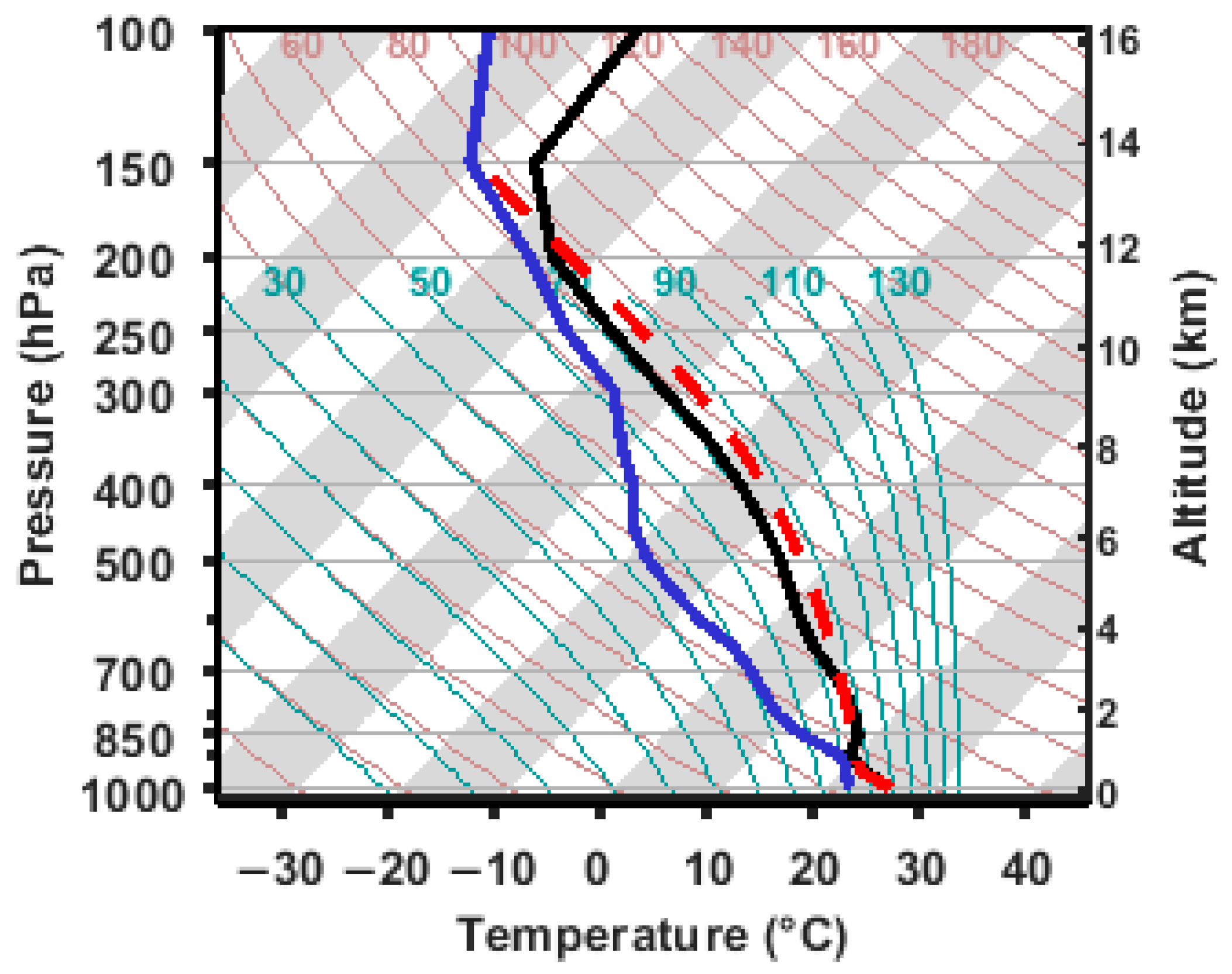
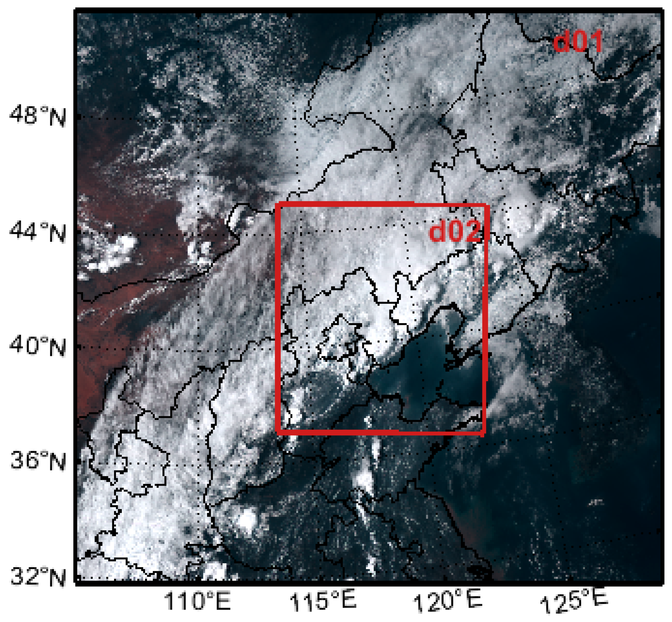
2.2. Overview of the Case

A squall line case occurred in the North China area on 18 August 2020 and produced heavy precipitation. This case is associated with a cold frontal system. The prefrontal sounding at 14:00 BJT (06:00 UTC) averaged for the region of 39–42° N and 117–121° E is shown in Figure 1, based on Final (FNL) reanalysis data (https://rda.ucar.edu/datasets/ds083.2/, accessed on 1 January 2020). The lower troposphere of this region has sufficient water vapor and a modest Convective Available Potential Energy (CAPE) of 850 J kg⁻¹ (parcels from the surface). The lifting condensation level is about 0.5 km at 21 °C. These conditions are favorable for convective triggering. The squall line was then triggered on the leading edge of the cold frontal system and developed into a mature stage in the period around 15:00–17:00 BJT. The squall line then moved in the northeast direction and started to decline. The early stage of this MCS is embedded in the cold frontal cloud. In the mature stage, the MCS moves faster than the cold frontal cloud and then separates. This type of MCS, triggered by cold frontal systems, occurs frequently in North China.

2.3. Model Setup

This squall line case is simulated with the Weather Research and Forecast (WRF) model, version 4.0 [55]. FNL reanalysis data with a horizontal resolution of 1° × 1° every 6 h are used as the initial field and lateral boundary conditions. The case is simulated from 02:00 to 20:00 BJT on 18 August 2020. Figure 2 shows the satellite cloud image at 15:00 BJT and the two nested domains designed for this study. The horizontal grid spacings of the domains are 9 and 3 km, respectively. The domains have 50 layers in the vertical direction, with resolutions of about 50~300 m in the boundary layer and 400~600 m in the free troposphere. Simulation results in domain 2 output every 10 min for the analysis of the structure and processes. All the simulations use the four-order Runge–Kutta algorithm on the time integration scheme, with a time resolution of 18 s. Morrison double-moment bulk microphysical scheme [56], Yonsei University boundary layer scheme [57], RRTM longwave radiation scheme [58], and Dudhia shortwave radiation scheme [59] are used in three domains. The Kain-Fritsch cumulus parameterization [60] is only used in domain 1. Details of the simulation setup can be seen in

Table 1. Simulation setup in the Weather Research and Forecasting model (WRF).

Parameters	Domain 1	Domain 2
Grid size (km)	9	3
Vertical resolution	σ-z terrain tracking coordinates; 50 layers; model top: 10 hPa;
Output time (min)	60	10
Microphysical scheme	Morrison	Morrison
Cumulus parameterization scheme	Kain–Fritsch	None
Boundary layer scheme	Yonsei University	Yonsei University
Longwave radiation scheme	RRTM	RRTM
Shortwave radiation scheme	Dudhia	Dudhia

.

The Morrison double-moment bulk microphysical scheme includes five hydrometeor species: cloud droplet, rainwater, ice crystal, snow, and graupel [56]. The cloud droplet concentration is set to be constant at 250 cm⁻³, which is a default value in the Morrison scheme. The number concentrations of the other hydrometeors are predicted. Mass concentrations are all predicted. All hydrometeors are assumed to be spheres with Marshall-Palmer distributions when calculating the microphysical process rates. The maximum number concentration of ice crystal uses the default value of 300 L⁻¹. A sensitivity test with the maximum number concentration of ice crystal to be 1000 L⁻¹ is also performed. The results show that this value does not affect the analysis of the effect of SIPs on concentrations of ice crystal (Figure S1) and precipitation rate (Figure S2).

In the Morrison scheme, ice crystals are produced by both primary ice processes (PIPs) and SIPs. PIPs, including homogeneous freezing of cloud droplets and heterogeneous nucleation (immersion freezing, contact freezing, and deposition and condensation freezing nucleation), are considered in the scheme. The parameterizations of PIPs are described in the Supplementary Materials (Text S1) in detail. For SIPs, only rime splintering was originally included in the scheme. Freezing drop shattering and ice-ice collisional breakup processes are added to the Morrison scheme in this study. Details of the SIP parameterizations are described in Section 2.4.

Table 2. Case description.

Case	Secondary Ice Productions (SIPs)
NOSIP	No SIPs
ALLSIP	Including all the three SIPs
RS	Only including rime splintering
DS	Only including freezing drop-shattering
CB	Only including ice-ice collisional breakup

is a summary of each case. This study mainly conducts a comparison between two simulations: one without SIPs (referred to as the NOSIP case) and another involving all three SIPs (referred to as the ALLSIP case). To dissect the individual effects and explore the relative importance of these three SIPs, three separate cases are simulated, each focusing on only one SIP. Specifically, the RS case only considers the rime splintering process, the DS case solely involves the freezing drop shattering process, and the CB case only includes the ice-ice collisional breakup process.

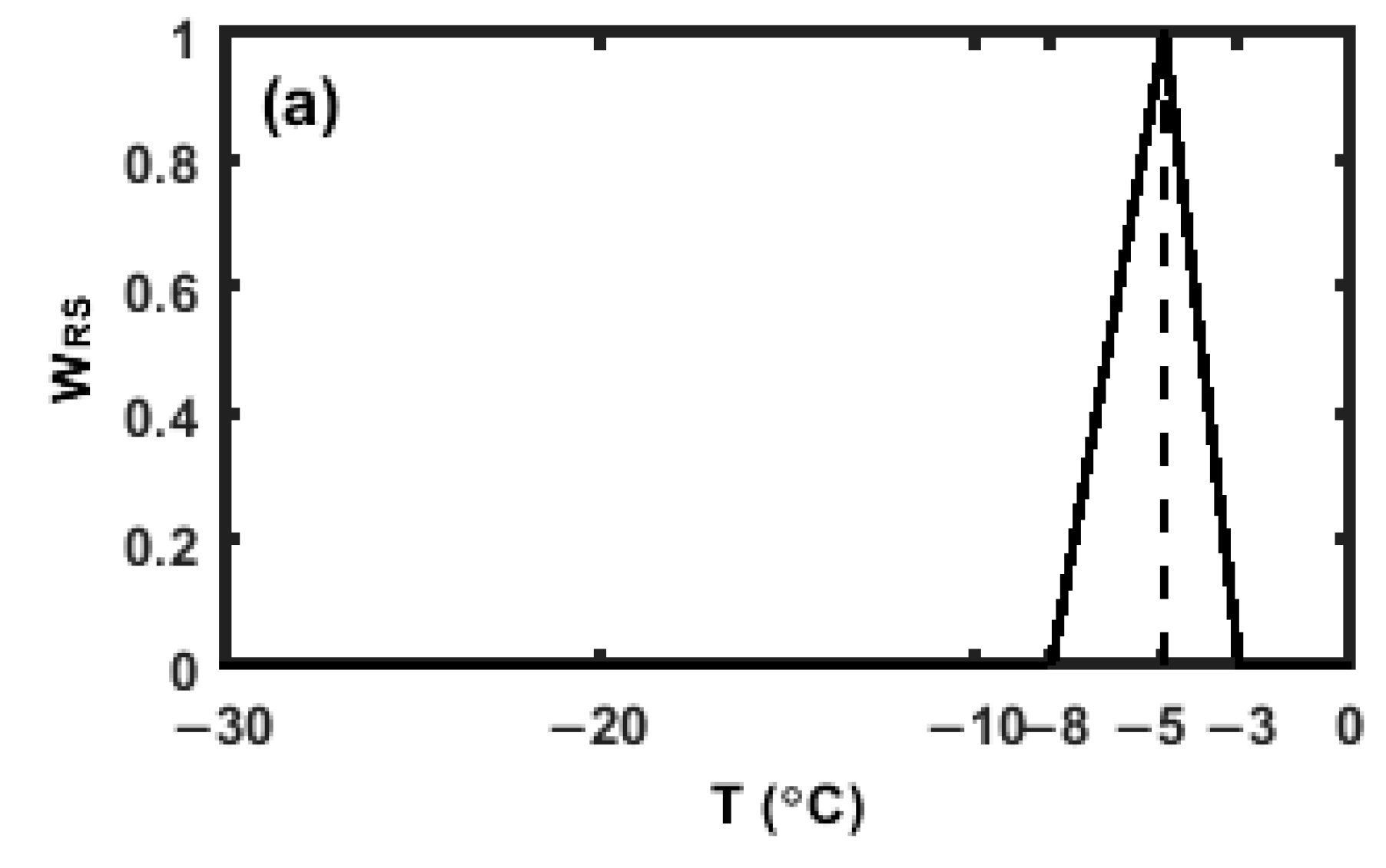
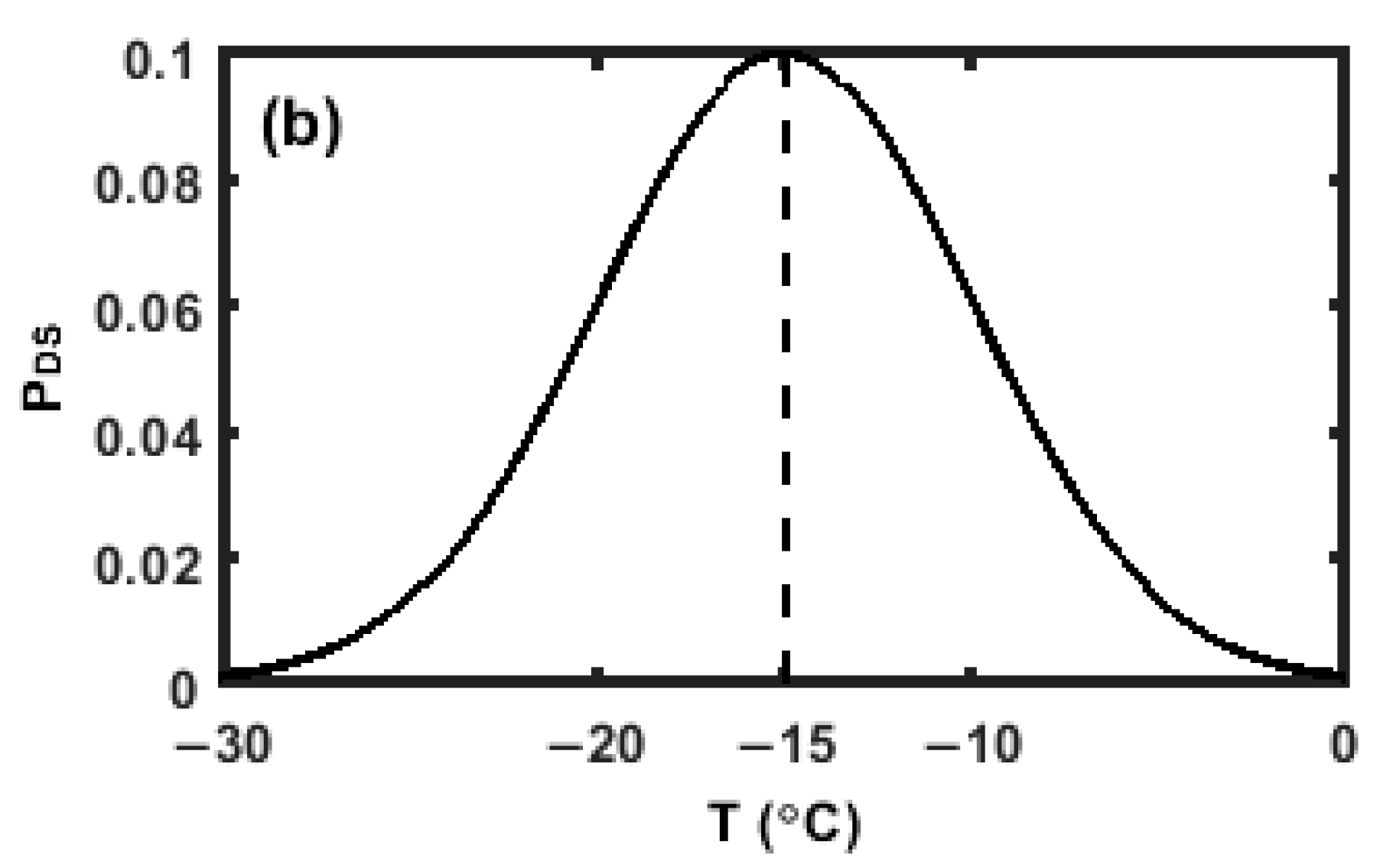
2.4. Parameterizations of SIPs

The rate of change of secondary ice number concentration through rime splintering is positively correlated with the rate of riming in the Morrison scheme and can be expressed as follows:

$$\frac{\partial n_{ice}}{\partial t}{|}_{RS}=w_{RS}{N}_{RS}\frac{\partial q_{rime}}{\partial t}$$

(1)

where $q_{rime}$ is the mass concentration of rimed droplets by snow and graupel [8]. The fragment number per milligram of rime, $N_{RS}$, is set to 3.5 × 10⁵. The weight function of ambient temperature, $w_{RS}$, has a form of piecewise linear distribution, which is set to 0 outside −3 to −8 °C and has a maximum value of 1 at −5 °C (Figure 3a). The secondary ice mass concentration is diagnosed using the number concentration, assuming all the ejected splinters have a diameter of 10 µm.

This study adds freezing drop shattering to the Morrison scheme using the parameterization format in Sullivan et al. [25], which assumes all freezing drops produce the same number of ice crystals and is applicable to bulk microphysics schemes. This treatment is not dependent on drop size, as in the bin schemes [21,22,39]. The rate of change of secondary ice number concentration through freezing drop shattering is as follows:

$$\frac{\partial n_{ice}}{\partial t}{|}_{DS}=\left[1+p_{DS}{N}_{DS}\right]\frac{\partial n_{freeze}}{\partial t}$$

(2)

where $n_{freeze}$ is the number of freezing drops. In Sullivan et al. [25], only immersion freezing is considered to calculate $n_{freeze}$. Korolev et al. [19] found that the number concentration of freezing drops measured above −4 °C cannot be explained by immersion freezing alone but also by ice-rain collisions in tropical maritime MCSs. Therefore, ice-rain collision (the parameterization is described in Supplementary Materials, Text S2) is also considered to calculate $n_{freeze}$ in this study, similar to Phillips et al. [22]. The fragment number by freezing drop shattering, $N_{DS}$, is set to 10, and the shattering probability, $p_{DS}$, is set to be a normal distribution of temperature centered at −15 °C with a maximum value of 10% and a standard deviation of 5 °C (Figure 3b), as in Sullivan et al. [25]. The mass concentration of secondary ice crystals through freezing drop shattering is calculated using the same method as in rime splintering in this study.

Parameterization of ice-ice collisional breakup is also added to the Morrison scheme in this study. The number and mass concentrations of ice crystals produced by ice-ice collisional breakup have the same format as in Phillips et al. [24]:

$$\frac{\partial n_{ice}}{\partial t}{|}_{CB}=N_{CB}·\frac{\partial n_{collision}}{\partial t}$$

(3)

$$\frac{\partial q_{ice}}{\partial t}{|}_{CB}=0.1\%·\frac{\partial q_{collided}}{\partial t}$$

(4)

where $N_{CB}$ is the breakup factor and represents the number of ice crystals produced by one collisional breakup, $n_{collision}$ is the total number of collisions between ice phase particles, and $q_{collided}$ is the mass of collided ice phase particles. In this study, there are five ice-ice collisional types: graupel-graupel, snow-graupel, ice crystal-graupel, snow-snow, and ice crystal-snow. The calculations of $N_{CB}$, $n_{collision}$, and $q_{collided}$ are summarized in

Table 3. The calculation method of three parameters in the equations of ice-ice collisional breakup rate. This study includes five collisional breakup types. Note that $N_{CB}$ is calculated based on Phillips et al. [24], while the $\frac{\partial n_{collision}}{\partial t}$ and $\frac{\partial q_{collided}}{\partial t}$ are calculated based on the method described in Sotiropoulou et al. [45].

Collision Type in this Study	${\mathit{N}}_{\mathit{C}\mathit{B}}$	$\frac{\partial {\mathit{n}}_{\mathit{c}\mathit{o}\mathit{l}\mathit{l}\mathit{i}\mathit{s}\mathit{i}\mathit{o}\mathit{n}}}{\partial \mathit{t}}$	$\frac{\partial {\mathit{q}}_{\mathit{c}\mathit{o}\mathit{l}\mathit{l}\mathit{i}\mathit{d}\mathit{e}\mathit{d}}}{\partial \mathit{t}}$
Graupel-Graupel	Type I in Phillips et al. [24]	Format in Passarelli [61], but with parameters of graupel instead of snow	Format in Verlinde et al. [62], but with parameters of graupel instead of snow
Snow-Graupel	Type II in Phillips et al. [24]	Format in Ikawa and Saito [63]	Format in Ikawa and Saito [63]
Ice crystal-Graupel	Type II in Phillips et al. [24]	Format in Reisner [64], but with parameters of graupel instead of raindrop	\
Snow-Snow	Type III in Phillips et al. [24]	Format in Passarelli [61], which is already concluded in default Morrison scheme	Format in Verlinde et al. [62]
Ice crystal-Snow	Type III in Phillips et al. [24]	Format in Reisner [64], but with parameters of snow instead of raindrop	\

.

$N_{CB}$ is calculated using the method in Phillips et al. [24] and has a format as follows:

$$N_{CB}=aA\left\{1-\exp \left[-{(\frac{C{K}_0}{aA})}^{\gamma }\right]\right\}$$

(5)

where $A$ is a measure of the number density (per unit area) of breakable vapor-grown branches or other asperities on the colliding surfaces in the region of contact,$\gamma$ is a power exponent, $C$ is the asperity-fragility coefficient (including a collection for sublimation effect), $a=\pi D^2$ is the equivalent spherical area of the collided particle, $K_0=\frac{1}{2}\frac{m_1{m}_2}{m_1+m_2}{\left(v_1-v_2\right)}^2$ is the collisional kinetic energy between two colliding particles. In Phillips et al. [24], the ice-ice collisions are categorized into three broad types, and each type has a set of parameters of $A$, $\gamma$, and $C$. Type I is the collision of graupel with graupel, where $A$ depends on temperature, and $\gamma$ and $C$ are two constants. Type II is the collision of ice crystals or snow with graupel, and Type III is the collision of ice crystals or snow with other ice crystals or snow. In Type II and Type III, $A$ and $\gamma$ are functions depending on the rimed fraction and habits of ice crystals and snow (either dendrite or planar), and $C$ is a constant.

When applying the method in Phillips et al. [24] to calculate the $N_{CB}$ in this study, graupel-graupel collision uses the type I parameters in Phillips et al. [24], snow-graupel and ice crystal-graupel collisions use the type II parameters, while snow-snow and ice crystal-snow collisions use the type III parameters in Phillips et al. [24]. Because all ice-phase particles are assumed to be spherical in the Morrison scheme, the calculations of $A$ and $\gamma$ for collisions involving ice crystal and snow use the functions for planar habit, which has a closer density and fall speed to the spherical shape of ice particles than the dendrites. $a$ and $K_0$ are calculated using the default spherical shape, fall velocity, and effective radius calculated from the Morrison scheme. The rimed fraction is not calculated in the Morrison scheme. Sensitivity tests on the rimed fraction indicate that the rimed fraction has little effect on ice crystal number concentration (Figure S3). The rimed fraction of ice crystal and snow is set to be 0.3 in this study, representing a moderately rimed condition.

$\frac{\partial n_{collision}}{\partial t}$ and $\frac{\partial q_{collided}}{\partial t}$ are predicted in the bin microphysics scheme in Phillips et al. (2017a). In this study,$\frac{\partial n_{collision}}{\partial t}$ and $\frac{\partial q_{collided}}{\partial t}$ are calculated using the method described in Sotiropoulou et al. [45]. Here we briefly describe the methods used for each of the five collision types. $\frac{\partial n_{collision}}{\partial t}$ by snow-snow is calculated in the original Morrison scheme when calculating the rate of snow aggregation. The calculation is based on Passarelli [61], which is related to the size distribution and fall speed of snow particles. $\frac{\partial q_{collided}}{\partial t}$ by snow-snow is added to the Morrison scheme and is calculated by the analytical solution for self-collection derived by Verlinde et al. [62], depending on the size distribution and fall speed parameters of snow particles. $\frac{\partial n_{collision}}{\partial t}$ and $\frac{\partial q_{collided}}{\partial t}$ by graupel-graupel is added to Morrison scheme using a similar method for the snow-snow collision, but with the size distribution and fall speed parameters replaced with those of graupel. $\frac{\partial n_{collision}}{\partial t}$ and $\frac{\partial q_{collided}}{\partial t}$ by snow-graupel are added to the Morrison scheme and are calculated based on Ikawa and Saito [63], which depends on the size distribution and fall speed parameters of snow and graupel. $\frac{\partial n_{collision}}{\partial t}$ by ice crystal-snow and ice crystal-graupel is added to the Morrison scheme and is calculated using the “continuous collection” approach based on Reisner [64], but with the size distribution and fall speed parameters replaced with those of snow or graupel. These two collision types do not change the mass of ice crystals, and therefore $\frac{\partial q_{collided}}{\partial t}$ does not need to be calculated.

3. Comparisons between the Observations and Simulations

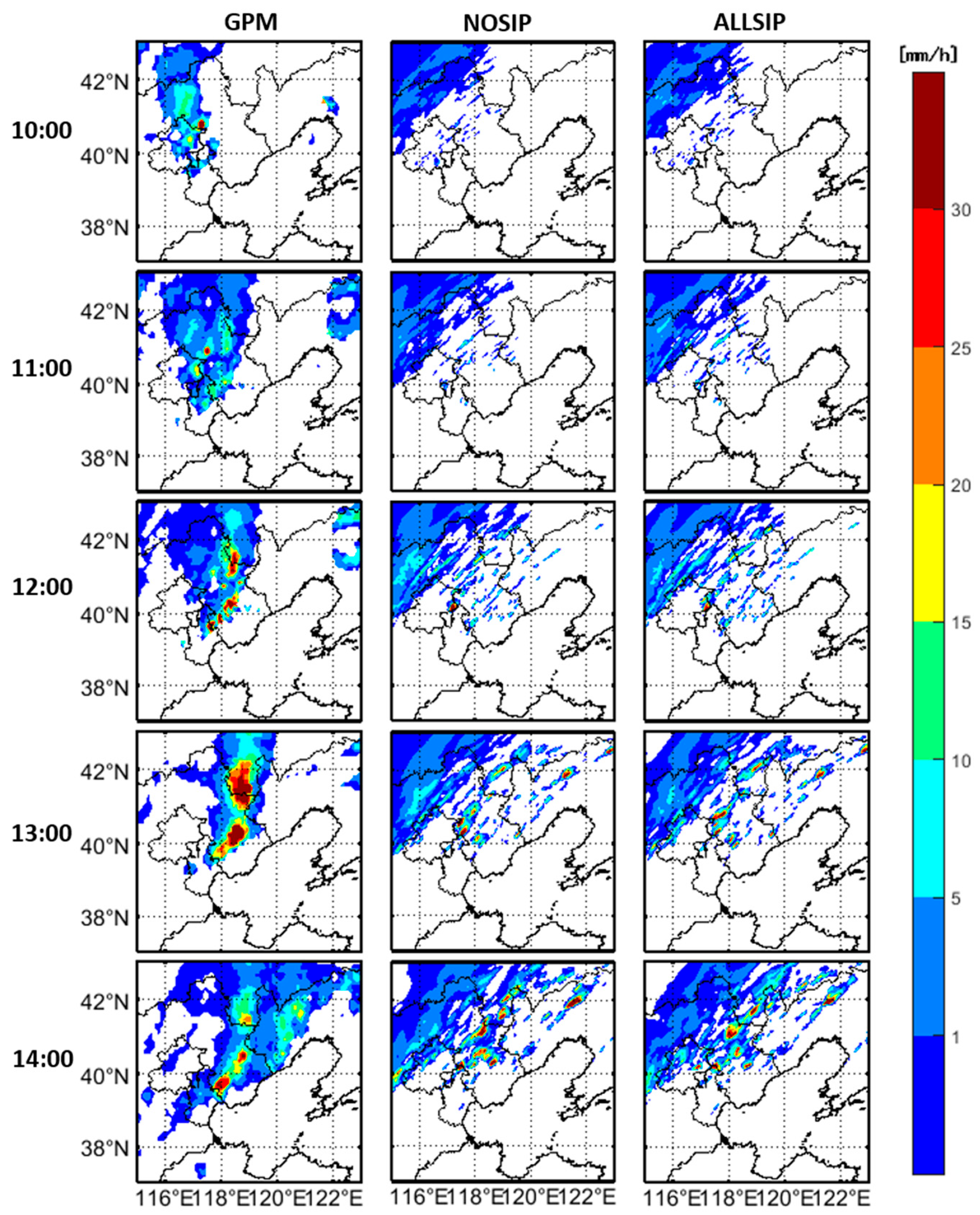
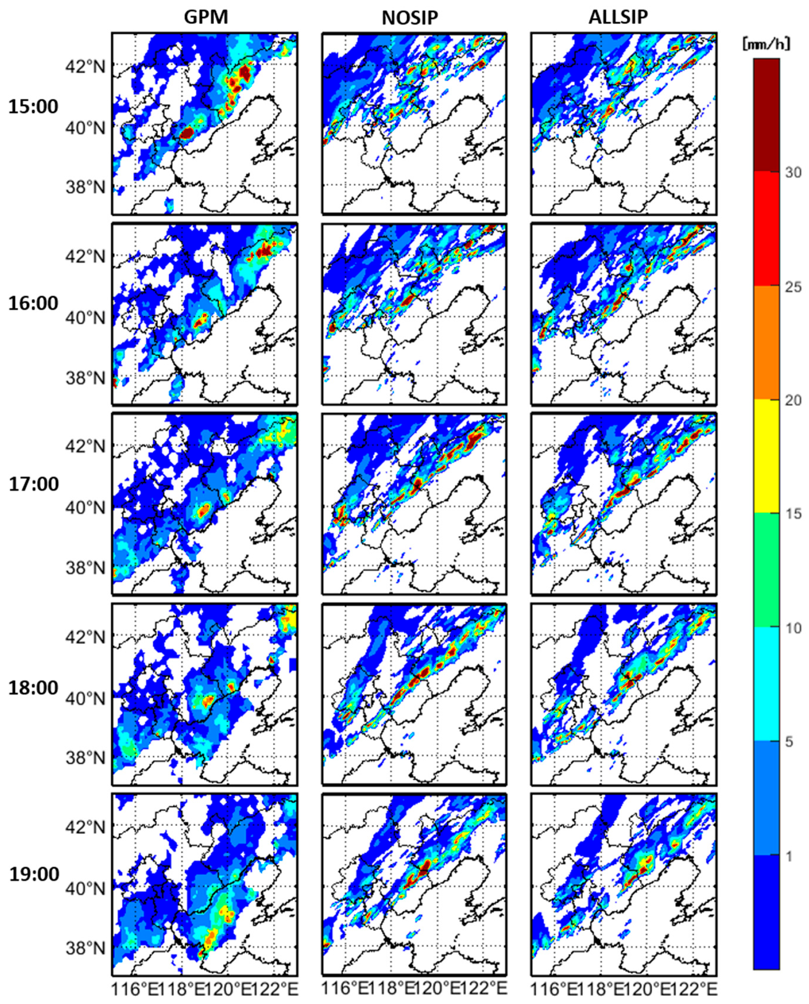
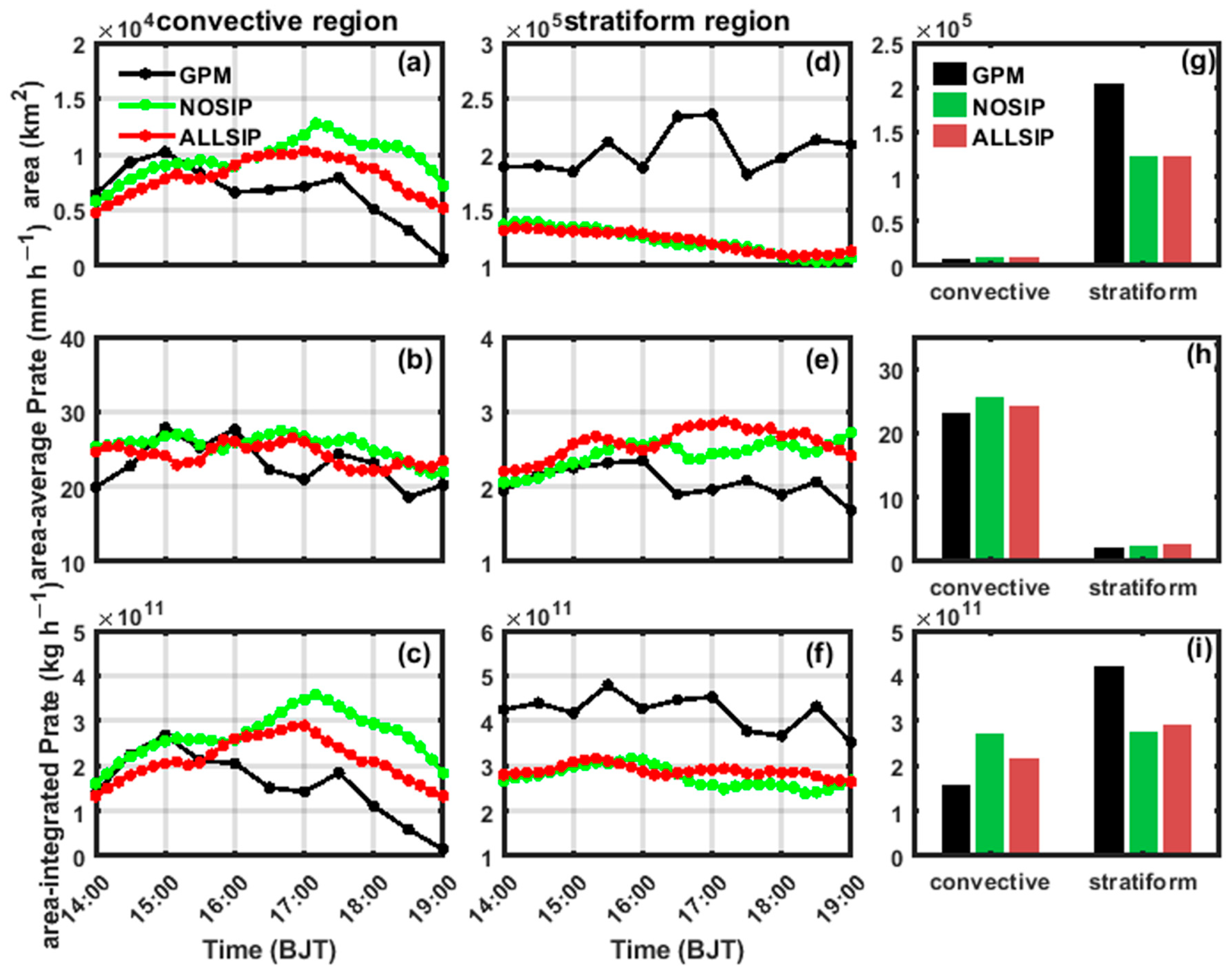
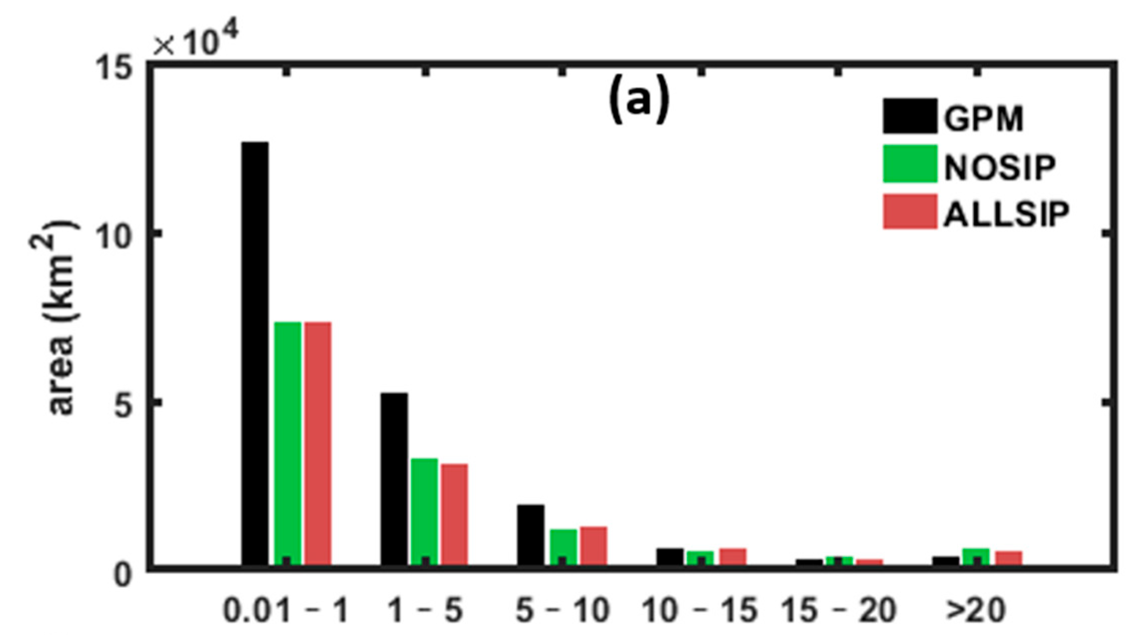
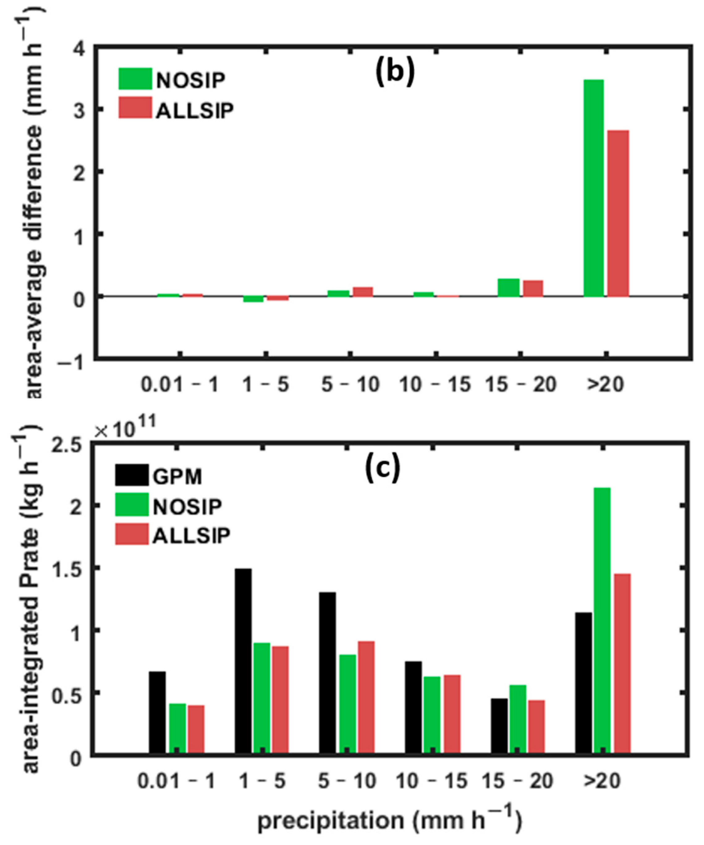
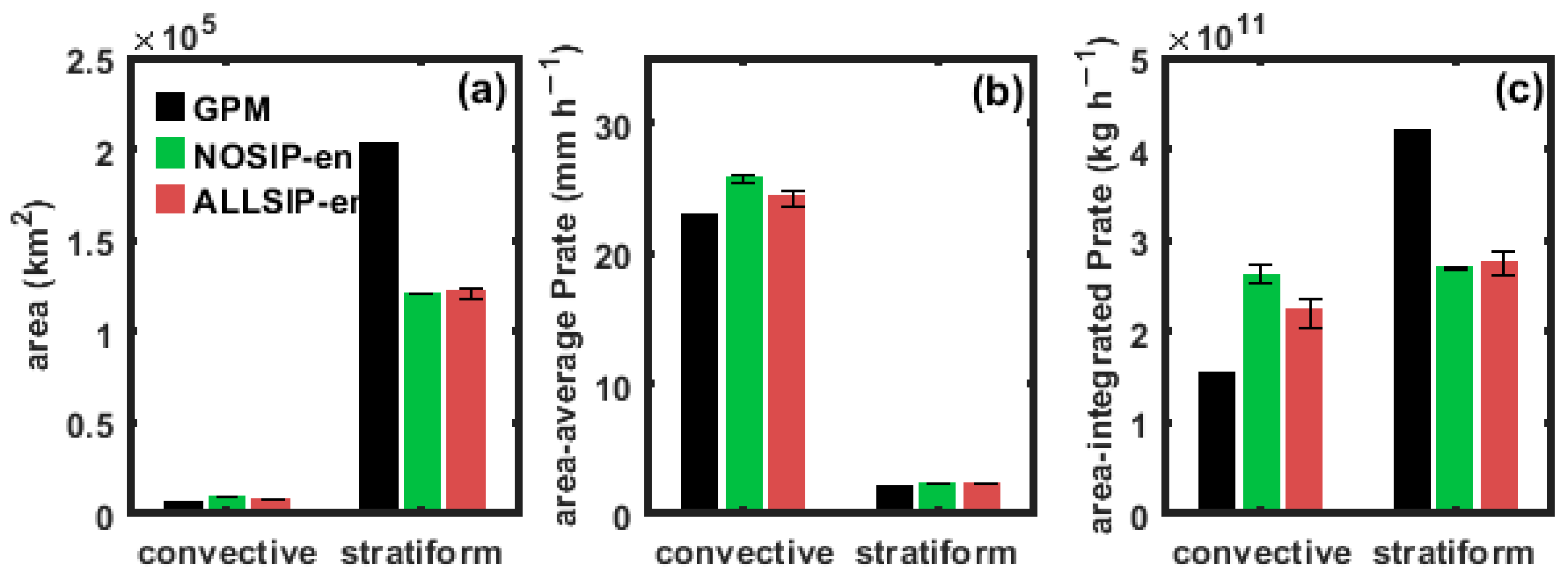
3.1. Comparison of Precipitation between Observations and Simulations

Figure 4 shows comparisons of the spatial distribution of the observed and simulated precipitation rates. 10 snapshots are shown from 10:00 to 19:00 BJT. The observed precipitation rate (the left column of Figure 4) shows that the organized convective clouds formed at 10:00 BJT and gradually intensified while moving in the northeast direction. These organized convective clouds continue to grow and line up as a very typical squall line from 15:00 to 17:00 BJT. This squall line begins to decline after 17:00 BJT. The simulated precipitation rate (the middle column for the NOSIP case and the right column for the ALLSIP case) generally shows a similar squall line system forming during the time period from 10:00 to 19:00 BJT, but the location of the simulated squall line is approximately 200 km to the west of the observed squall line, and the time is about 2 h late. The simulated convective clouds line up and develop into a typical squall line during 17:00 to 19:00 BJT, which closely resembles the observed squall line during 15:00 to 17:00 BJT.

In Figure 5, we focus on the precipitation area, area-averaged precipitation rate, and area-integrated precipitation rate (precipitation mass in the region per hour, a multiplication of precipitation area, area-averaged precipitation rate, and water density) during 14:00 to 19:00 BJT, which covers the typical squall line period. The precipitating area is partitioned into the convective region and stratiform region of the squall line. The observed and simulated precipitation properties are compared in each region. A precipitation rate threshold in the range of 10–25 mm h⁻¹ has been used in the literature for partitioning convective and stratiform regions of squall lines [65]. Here, in this study, we use a precipitation rate threshold of 15 mm h⁻¹. The convective region is defined as the strong precipitation area (precipitation rate above 15 mm h⁻¹), and the stratiform region is defined as the weak precipitation area (precipitation rate below 15 mm h⁻¹ and larger than 0.01 mm h⁻¹). 10 mm h⁻¹ and 20 mm h⁻¹ are also tested as the thresholds for partitioning convective and stratiform regions, and the results are shown in Figure S4 and S5. Regardless of the threshold used, the convective area is one order of magnitude smaller than the stratiform area, and the ALLSIP case shows a better simulation of the precipitation in the convective region. Details will be shown below.

For the convective region, it is seen in Figure 5a that the observed and simulated convective areas all reach their maximum during 14:00–19:00 BJT. The maximum of the observed convective areas appears at 15:00 BJT, while the maximum of the simulated convective area appears at 17:10 BJT for the NOSIP case and 17:00 BJT for the ALLSIP case, about 2 h later than the observed, as has been seen in Figure 4. The maximum of the convective area is respectively 1.02 × 10⁴, 1.27 × 10⁴, and 1.03 × 10⁴ km² in the observation, NOSIP case, and ALLSIP case. The time-averaged convective area is shown in Figure 5g and is, respectively, 6.51 × 10³, 9.63 × 10³, and 8.03 × 10³ km² in the observation, NOSIP case, and ALLSIP case. The root-mean-square error between the ALLSIP case and observation is 2.86 × 10³ km², and that between the NOSIP case and observation is 4.11 × 10³ km². The convective area in the ALLSIP case is closer to the observation in terms of the maximum and time-averaged convective area, as well as the root-mean-square error.

The observed and simulated area-averaged precipitation rates in the convective region all show typical pulsating features on a time scale of about 1 h but are out of phase (Figure 5b). The time-averaged precipitation rate during 14:00 to 19:00 BJT is, respectively, 23.01, 25.47, and 24.19 mm h⁻¹ in the observation, NOSIP, and ALLSIP cases (Figure 5h). The precipitation rate simulated by the ALLSIP case is also closer to the observation, and the root-mean-square error between the ALLSIP case and observation is 3.27 mm h⁻¹, which is also smaller than that between the NOSIP case and observation (3.4 mm h⁻¹).

The area-integrated precipitation rate in the convective region, which is governed by both the convective area and the precipitation rate, is shown in Figure 5c. The area-integrated precipitation rate in the ALLSIP case is closer to the observed, as expected. In general, including SIPs improves the simulated convective area and precipitation rate in the convective region.

For the stratiform region, Figure 5d–f shows the observed and simulated area, area-averaged precipitation rate, and area-integrated precipitation rate. Both the NOSIP case and the ALLSIP case underestimate the stratiform area (Figure 5g) and overestimate the area-averaged precipitation rate (Figure 5h) in the stratiform region, which can also be seen in Figure 4. The area-integrated precipitation rate in the stratiform region simulated by NOSIP and ALLSIP cases is both less than the observed rate (Figure 5i). The underestimation of the stratiform area has been a common issue in the model simulation of squall lines [56,66,67,68,69]. Here, in this study, including SIPs does not improve the simulation of the stratiform area or the precipitation rate in the stratiform region.

Figure 6 shows the histogram of the precipitation in six bins. We have shown in Figure 5 that including SIPs can improve the precipitation averaged in the convective region but does not improve the precipitation averaged in the stratiform region. Here we classify the precipitation rate into six bins and compare the simulations and observations in each bin between 14:00 and 19:00 BJT. Figure 6a shows the precipitation area, Figure 6b shows the difference in the area-averaged precipitation rate between the simulated case and the GPM observation, and Figure 6c shows the area-integrated precipitation rate. For each bin in the convective region (precipitation rate in the range of 15–20 and >20 mm h⁻¹), the ALLSIP case improves the simulation of the convective area, area-averaged precipitation rate, and area-integrated precipitation rate. For each bin in the stratiform region (precipitation rate in the range of 0.01–1, 4, 5–10, and 10–15 mm h⁻¹), the ALLSIP case nearly does not improve the simulation of stratiform area, area-averaged precipitation rate, and the area-integrated precipitation rate. For the bin with a precipitation rate of 0.01–1 mm h⁻¹, the precipitating area contributes most to the area of the stratiform region. The simulated area in this bin in the NOSIP case and the ALLSIP case is significantly smaller than that observed, which may explain the large difference in stratiform area between simulations and observations in Figure 5d. In general, considering SIPs in the model indeed improves the simulation of the convective area and precipitation rate in each bin of the convective region and therefore shows better model performance in simulating the convective area.

Three cases, including single SIP (RS, DS, and CB), also improve the simulations of convective area, area-average precipitation rate, and area-integrated precipitation rate in the convective region, but do not improve the simulations in the stratiform region (Figure S6). The CB case has a better simulation of the convective region compared to the RS case and the DS case. But it can be seen that none of these cases can simulate the convective region as well as the ALLSIP case.

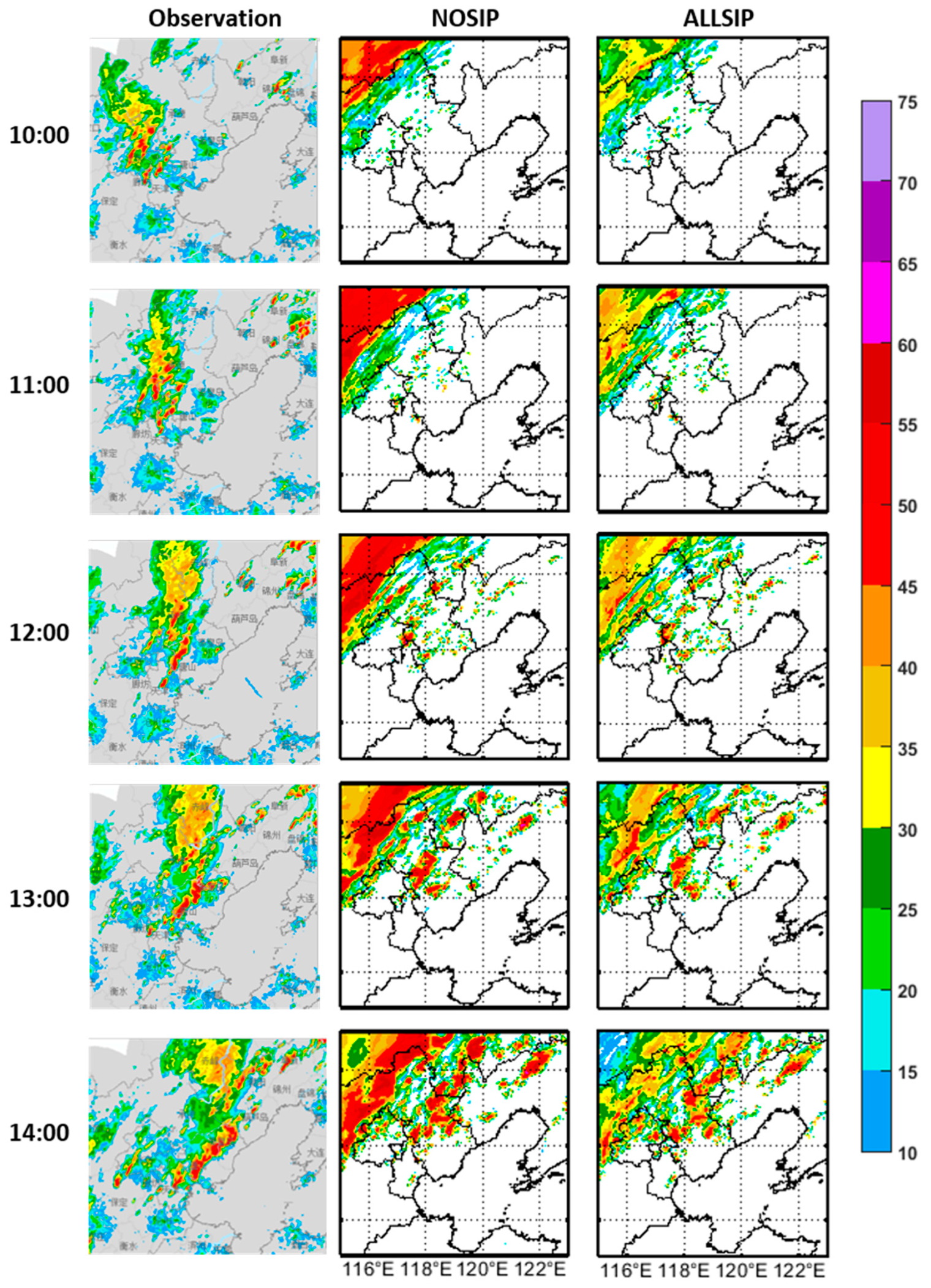
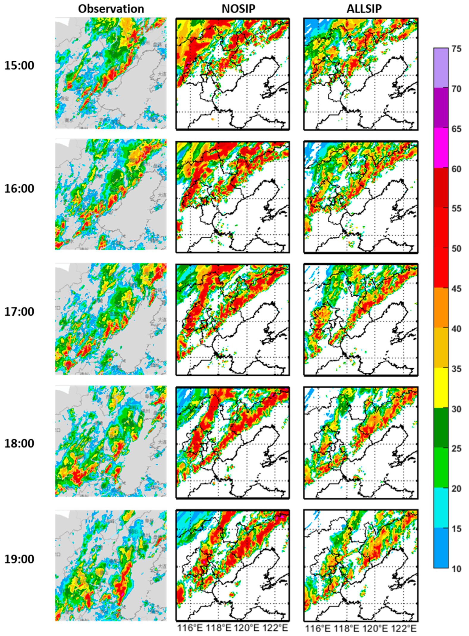
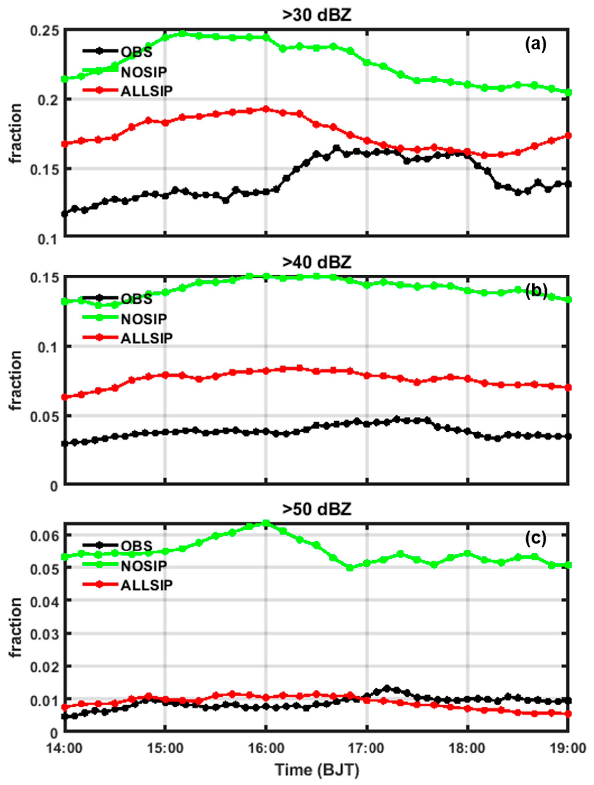
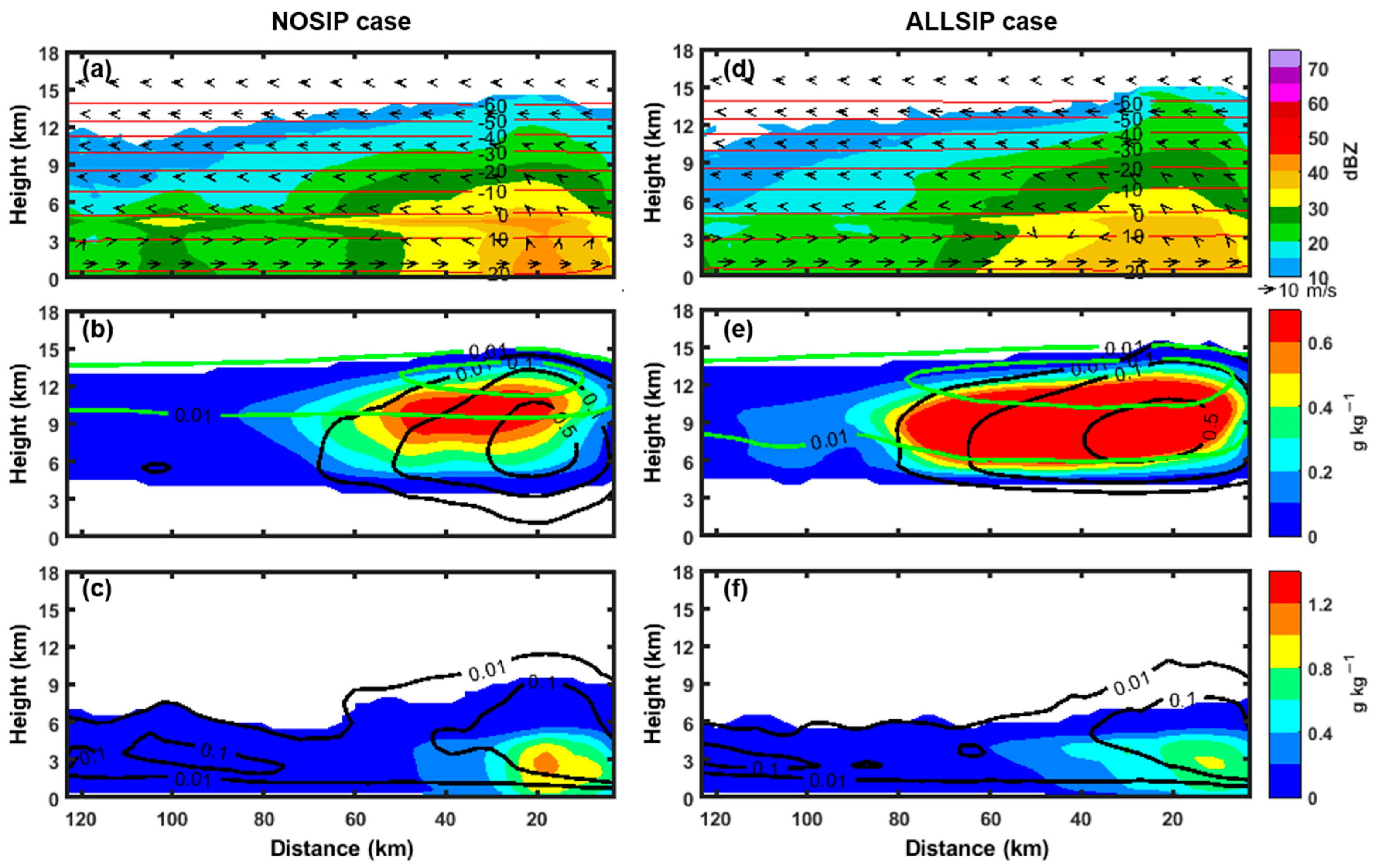
3.2. Comparison of Radar Reflectivity between Observations and Simulations

Any overestimation of strong precipitation by the model might not necessarily be incorrect, as it could be attributed to observational uncertainty, as highlighted by Shahi [70]. To address this, we conducted a comparison between simulated and observed radar reflectivity. Figure 7 presents a spatial distribution comparison of observed and simulated composite radar reflectivity, featuring 10 snapshots from 10:00 to 19:00 BJT—covering the same time period as the precipitation comparison in Figure 4. The composite radar reflectivity, calculated following Stoelinga [71], reveals that the location and timing of the simulated squall line are posterior to the observed and positioned westward, aligning with the spatial distribution of precipitation rate (Figure 4). A noteworthy observation is the distinct feature where the area with composite radar reflectivity exceeding 50 dBZ (indicating strong convections and strong precipitation) in the ALLSIP case closely aligns with the observation. In contrast, the NOSIP case exhibits a significantly larger area with reflectivity exceeding the observation and the ALLSIP case across all 10 snapshots.

The composite radar reflectivity in observations and simulations between 14:00 and 19:00 BJT is classified into six bins. The ratio of the area of each bin to the total area of the studied region is compared between observations and simulations. For the observation, the area for each bin and the total area of the studied region are obtained using the image recognition technique because we only have images of radar reflectivity. We manually select the area in the image to replicate the simulated area (37° N–43° N and 115° E–123° E) as close as possible, as can be seen in Figure 7. It is found that the fraction of area for each bin does not significantly alter when shifting the studied region in the simulated radar reflectivity by 0.5° to the east, west, south, and north of 37° N–43° N and 115° E–123° E (Figure S7). This suggests that the slight difference between the studied area in the simulations and observation has little impact on the results of the above analysis.

Figure 8 shows the histogram of the composite radar reflectivity in 6 bins from 14:00 to 19:00 BJT. The fraction of area for each bin simulated by the ALLSIP case is closer to the observation, especially in the bins of 50–60 dBZ, as already seen in Figure 7. For the bins of 40–50 dBZ and 50–60 dBZ, the NOSIP case overestimates the fraction of area by a significant amount. For the bins of 10–20 dBZ, 20–30 dBZ, and 30–40 dBZ, the NOSIP case underestimates the fraction of the area. Note that large composite radar reflectivity usually exists in the convective region with relatively strong precipitation. Results shown in Figure 8 are consistent with the results shown in Figure 8 that the ALLSIP case has a better simulation of the convective area (defined as precipitation rate larger than 15 mm h⁻¹) and that the NOSIP case overestimates the convective area by a significant amount (Figure 8a). Small composite radar reflectivity usually belongs to the stratiform region. It is seen in Figure 8 that the fraction of area for smaller radar reflectivity is still underestimated even after adding SIPs. The underestimation of the stratiform area has been a common issue in the model simulation of squall lines, which has also been discussed in Figure 5. Processes other than SIPs should be considered to resolve this issue.

We now investigate if the ALLSIP case has a better simulation at all snapshots in the convective region. Figure 9 shows the time series of the fraction of area with radar reflectivity larger than 30 dBZ, 40 dBZ, and 50 dBZ. These dBZ thresholds tend to represent convective regions of the squall line. At each snapshot between 14:00 and 19:00 BJT, the fraction of the convective area simulated by the ALLSIP case is closer to the observation than the NOSIP case. This time-resolving result in Figure 9 is in agreement with the histogram analysis in Figure 8.

Considering the contrast between precipitation and radar reflectivity, including SIPs indeed can improve the simulation of the convective area and precipitation rate in the convective region. This indicates that future simulations of squall lines should consider SIPs in the models. However, it is noteworthy that the simulation tends to underestimate the stratiform area, and despite including SIPs, there is no observable improvement in simulating the stratiform region.

3.3. Model Uncertainty

In order to prove that the better simulation of the convective area and precipitation rate in the convective region in the ALLSIP case is caused by including SIPs in the model rather than the model uncertainty, five additional ensemble simulations are performed, respectively, in the NOSIP case and the ALLSIP case. The initial temperature field at each grid point is perturbed randomly, ranging from −1 K to +1 K, as the model setting in Qu et al. [33]. Figure 10 shows the time average of precipitation area, time- and area-averaged precipitation rate, and the time-average of area-integrated precipitation rate of the convective and stratiform regions for the GPM observation, 6 ensembles of the NOSIP case, and 6 ensembles of the ALLSIP case. The 6 ensemble results are very consistent with each other. It can be seen in Figure 10 that the error bars of the 6 ensembles are very small. The difference between ensemble simulations is smaller than the difference between the NOSIP case and the ALLSIP case in the convective region. This indicates that including SIPs indeed improves the simulations of convective area and precipitation rate in the convective region in this case. The microphysical feedbacks that lead to improved precipitation and radar reflectivity in the ALLSIP case are analyzed below.

4. Microphysical Properties and Feedback

4.1. General Features of the Simulated Cases

Figure 11 shows the time-averaged cross-sections for the NOSIP and ALLSIP cases. To get a time-averaged cross-section, we first define the leading edge of the storm at each snapshot as the leading line that is oriented in the northeast-southwest direction and also passes a maximum radar reflectivity of 35 dBZ. We then get a time-averaged cross-section based on the relative distance to the leading edge of the storm for all 13 snapshots between 17:00 and 19:00 BJT, as can be seen in Figure 11. Cross sections for single snapshots are shown in Figures S8–S10 for reference.

For both the NOSIP case and the ALLSIP case, the simulated squall line has a cloud top height of about 15 km, the −38 °C layer at about 11 km, and the 0 °C layer at about 5 km (Figure 11a,d). Here, we can define the layer above 11 km as the anvil layer. The layer at 5–11 km can be defined as the mixed-phase layer. The layer below 5 km can be defined as the warm layer. Note that the definition of the mixed-phase layer here does not imply that every grid in this layer is mixed-phase. The definition here mainly considers the height range and temperature range that are possibly mixed-phase for the convenience of analysis. As can be seen in Figure 12a, the fraction of the grids that are mixed-phase (with both liquid and ice phase particles) can be as high as 89% at about 6 km. The WBF process typically only occurs in regions where the air is supersaturated over ice but subsaturated with water in the mixed-phase layer [72]. Figure 12b shows the fraction of the grids satisfying both the conditions of subsaturation for liquid water and supersaturation for ice, and Figure 12c shows the fraction of the grids where the WBF process could occur. The WBF process only occurs in less than 50% of the grids in the mixed-phase layer.

Figure 11a,d shows that the maximum radar reflectivity in each column is distributed mainly in the warm layer (below 5 km). The anvil layer (above 11 km) mainly contains ice crystals and a little amount of snow and graupel (Figure 11b,e). The mixed-phase layer (5–11 km) mainly contains snow and graupel and also contains some supercooled water. The warm layer mainly contains rainwater and cloud water (Figure 11c,f), as well as melting snow and graupel.

The time-averaged cross sections in the ALLSIP case (Figure 11d–f) have some differences in the mixed-phase layer and warm layer compared with the NOSIP case (Figure 11a–c). In the mixed-phase layer (5–11 km), a very interesting feature is that the ALLSIP case has significantly higher radar reflectivity than the NOSIP case (Figure 11d), due to the significantly increased snow (Figure 11e). The mass of ice crystals is also increased in the mixed-phase layer in the ALLSIP case compared with the NOSIP case. In the warm layer, the radar reflectivity and rainwater mass are decreased in the ALLSIP case (Figure 11d,f). The smaller radar reflectivity in the ALLSIP case in the warm layer is consistent with the smaller composite radar reflectivity in the ALLSIP case as seen in Figure 7. The decreased rainwater and graupel mass account in the ALLSIP case account for the smaller radar reflectivity, compared with the NOSIP case. The difference in the hydrometeor concentrations between the two simulations and the related microphysical mechanisms will be discussed in detail below.

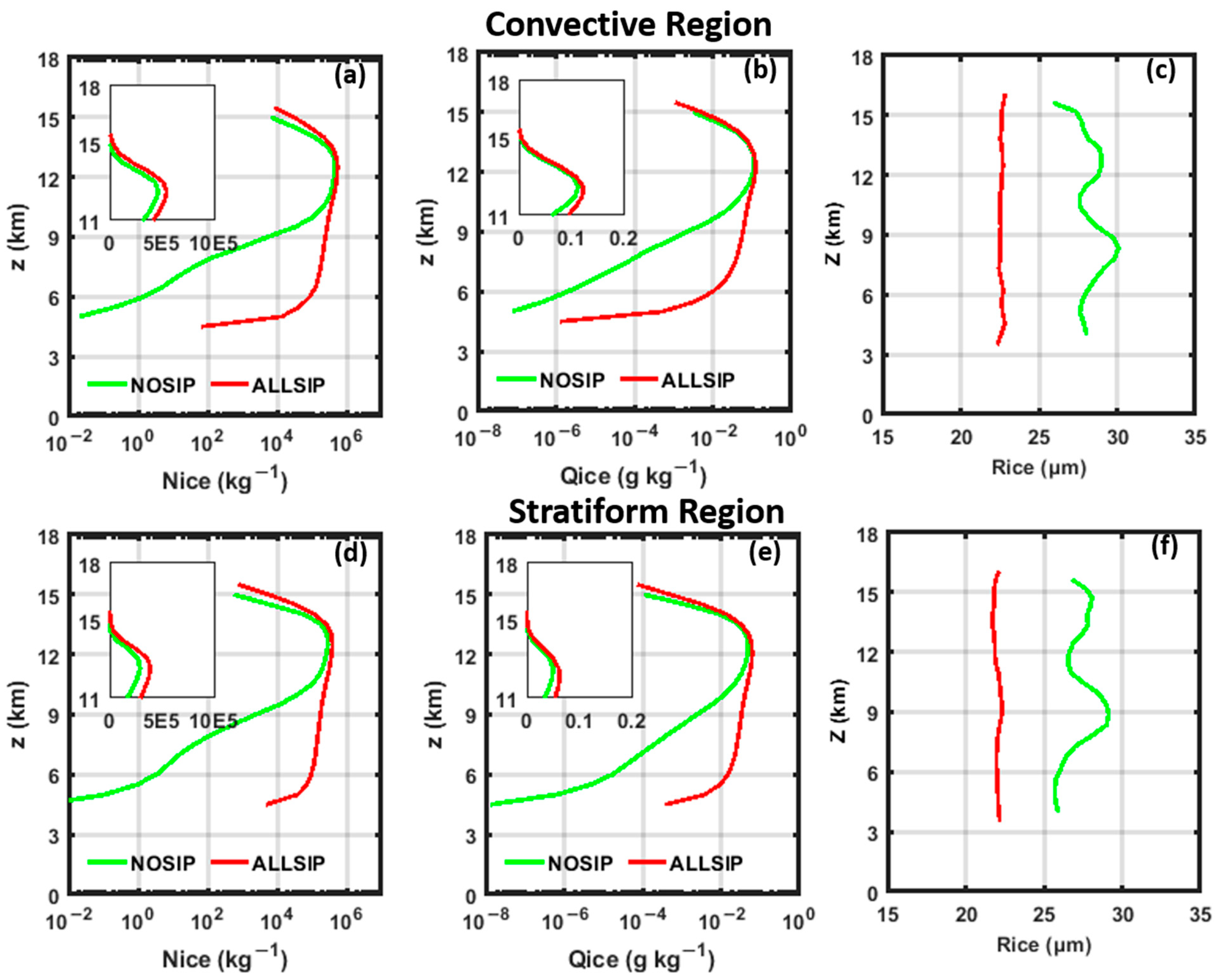
4.2. Ice Crystal Properties

Figure 13 shows the ice crystal number concentration (a,d), mass concentration (b,e), and effective radius (c,f) averaged over the convective region and stratiform region for the five cases. The number and mass concentrations of ice crystals progressively increase in the DS, RS, and CB cases in the mixed-phase layer, for both the convective and stratiform regions. This indicates that ice-ice collisional breakup plays the most significant role in ice crystal production among the three SIPs. The DS case can produce ice crystals with a similar number, mass concentration, and effective radius as the NOSIP case, while the CB case is similar to the ALLSIP case. The RS case produces an ice crystal number and mass concentration that is one order of magnitude lower than that in the ALLSIP case. This also suggests that freezing drop shattering played little role in this squall line case, while ice-ice collisional breakup played the dominant role, almost covering the role of rime splintering. Below, only the microphysical properties in the NOSIP and ALLSIP cases are analyzed in detail.

In the convective region, as can be seen from Figure 13a,b, SIPs in the ALLSIP case lead to the most pronounced increase of ice number and mass concentrations by about 5 orders of magnitude at the −8 °C (~6 km) level, compared to the NOSIP case. The number and mass concentration of ice crystals increase by 27% (inset of Figure 7a) and 7% (inset of Figure 13b) in the anvil layer, with the effective radius decreasing by 19% (Figure 7c), which means that there are more but smaller ice crystals in the anvil layer. In the stratiform region, SIPs also increase the number and mass concentrations of ice crystals most significantly at the −8 °C (~6 km) level, by 5 and 4 orders of magnitude, respectively (Figure 13d,e). The number and mass concentrations in the anvil layer increase by 47% and 33%, respectively, and hence the effective radius of ice crystals decreases by 18% (Figure 7f).

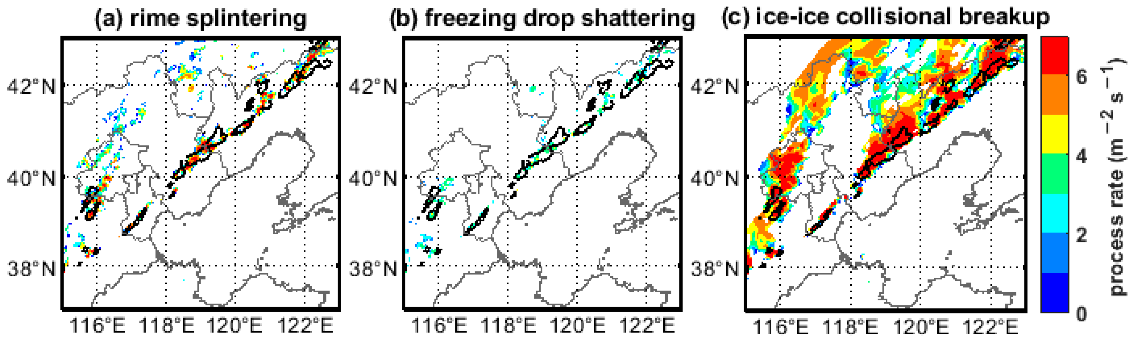
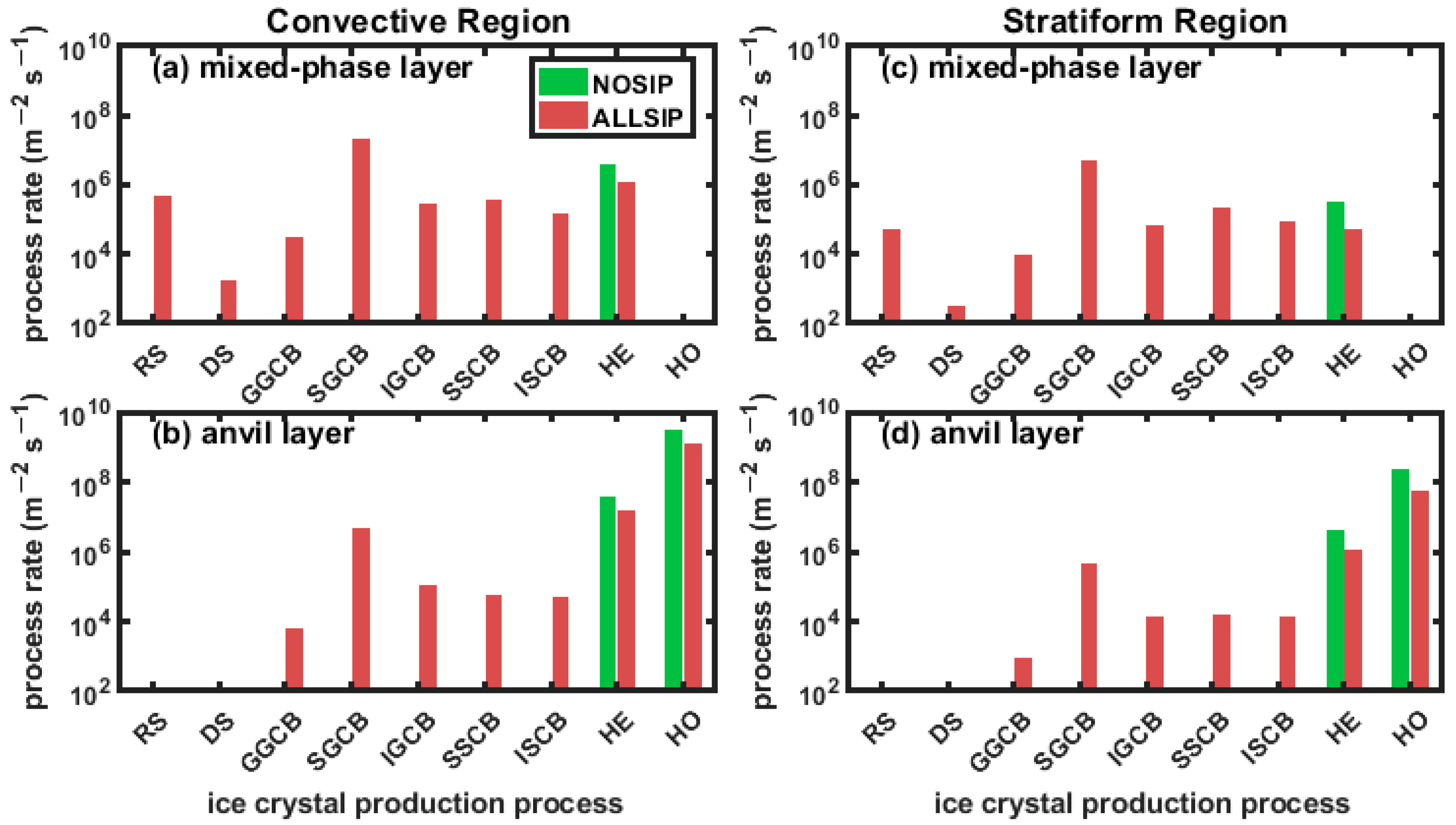
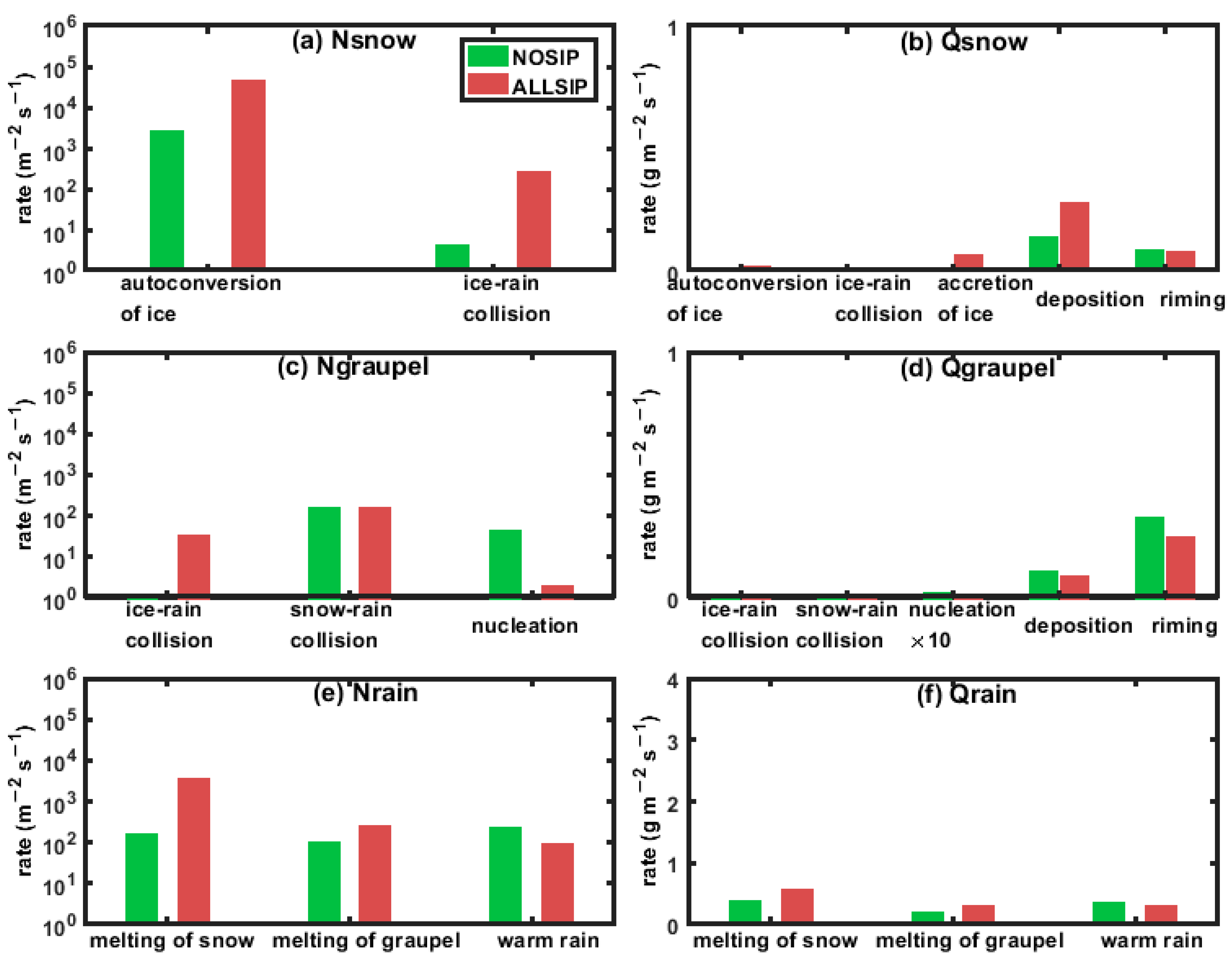
4.3. Secondary and Primary Ice Production Rates

Now we focus on the ALLSIP case to study the SIPs and their contributions to ice production. Figure 14 shows the spatial distribution of the vertically averaged rates of three SIPs in the ALLSIP case. Rime splintering and freezing drop shattering occur mainly in the convective region and only in limited areas of the stratiform region (Figure 14a,b), and also have rates at least one order of magnitude lower than ice-ice collisional breakup. This is because supercooled water is required in the rime splintering and freezing drop shattering. In contrast, the ice-phase particles are spread throughout the squall line (Figure 11e) therefore, ice-ice collisional breakup extensively occurs in both the convective and stratiform regions (Figure 14c). However, the rate of ice-ice collisional breakup in the convective region is about an order of magnitude larger than that in the stratiform region.

Figure 15 shows the rates of SIPs and PIPs averaged over the convective region and the stratiform region. In the mixed-phase layer of the convective region, rime splintering produces only 3% of ice crystals, freezing drop shattering contributes less than 1%, while ice-ice collisional breakup of snow-graupel produces 90% of ice crystals, which is at least one order of magnitude higher than the other types of collisional breakup. SIPs produce ice crystals much more than PIPs from heterogeneous nucleation (5%) (Figure 15a). In the anvil layer of the convective region, rime splintering and freezing drop shattering do not occur, and collisional breakup contributes less than 1% to ice production. PIPs dominate over SIPs in ice production (Figure 15b). The process that produces the most ice crystals is homogeneous nucleation of cloud droplets (98%), rather than heterogeneous nucleation (1%).

In the mixed-phase layer of the stratiform region, supercooled cloud water and graupel are less than that in the convective region (see Figure 11e, f), so rime splintering produces only 1% of ice crystals, and freezing drop shattering contributes less than 1% (Figure 15c), which is consistent with Figure 14. Ice crystal production is also dominated by ice-ice collisional breakup of snow–graupel (90%). In the anvil layer of the stratiform region (Figure 15d), the ice crystal production rate is about an order of magnitude smaller than in the convective region. Homogeneous nucleation of cloud droplets also contributes most to the ice crystal number concentration (97%), which is consistent with the convective region.

In the NOSIP case, only the PIPs occur. For both the convective region and stratiform region, ice crystals in the mixed-phase layer are generated by the heterogeneous nucleation process, but ice crystals in the anvil layer are mainly generated by the homogeneous nucleation process. Compared with the NOSIP case, the PIP rates in the ALLSIP case can be reduced by SIPs in both the mixed-phase layer and the anvil layer (Figure 15). The relevant microphysical feedback will be explained in Section 4.4.

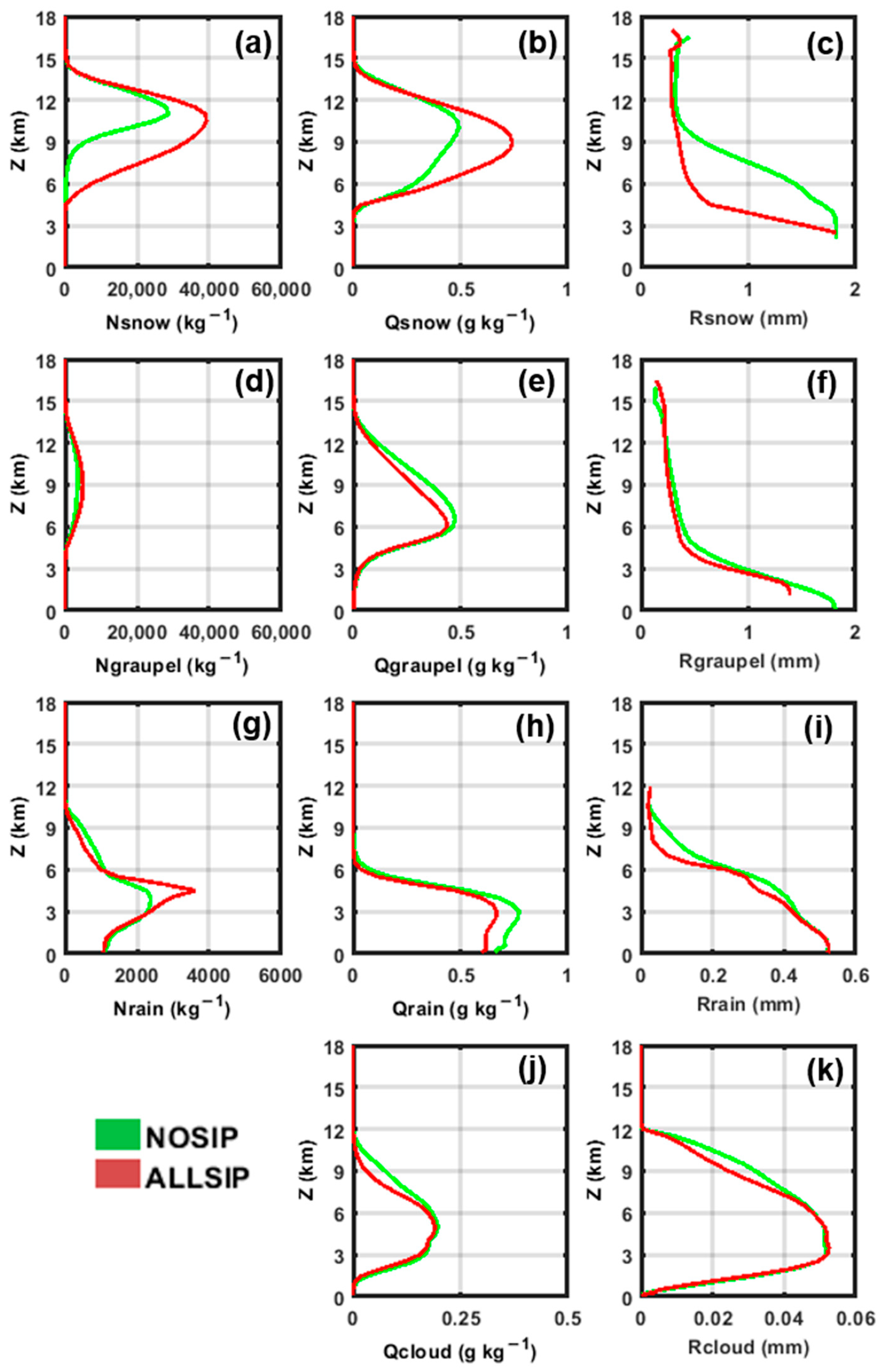
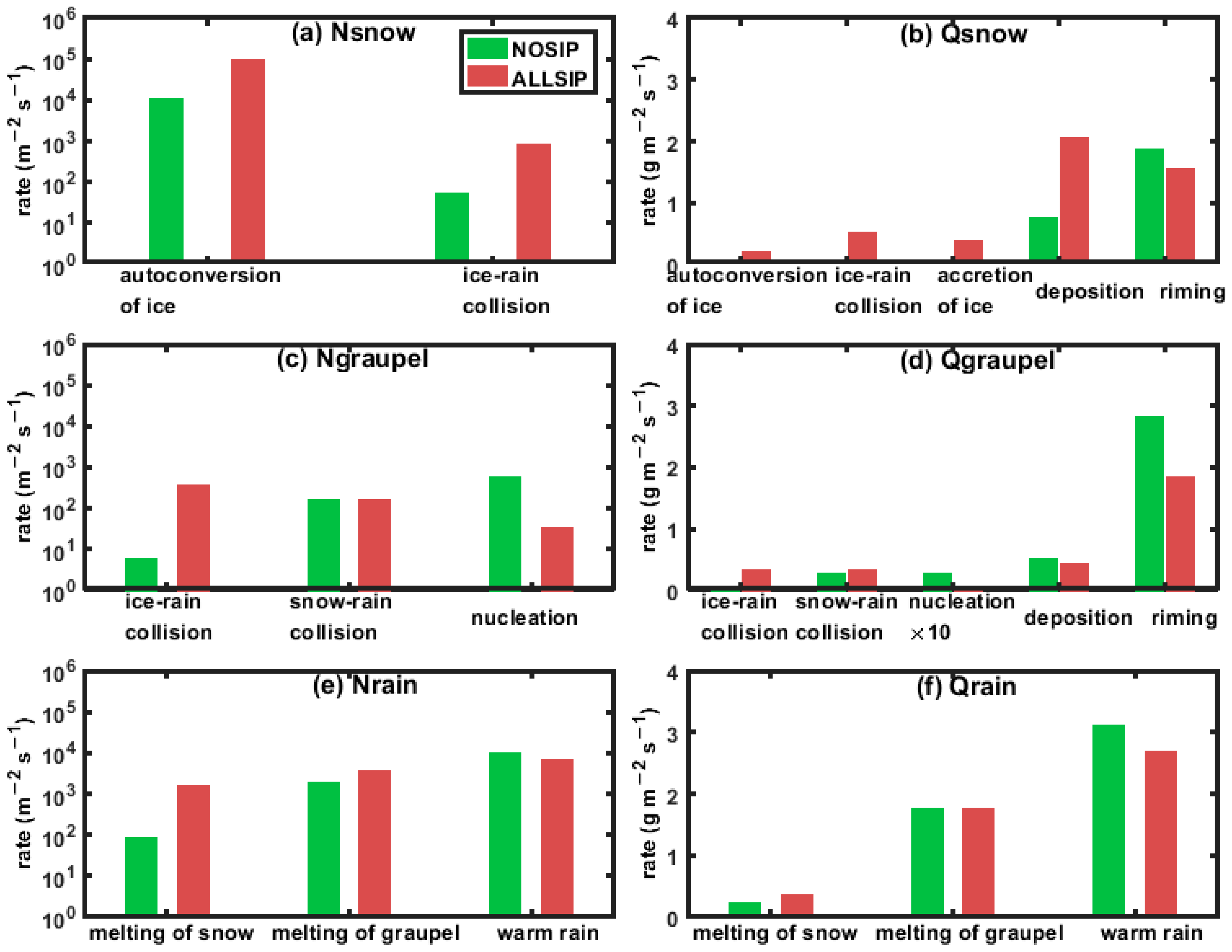
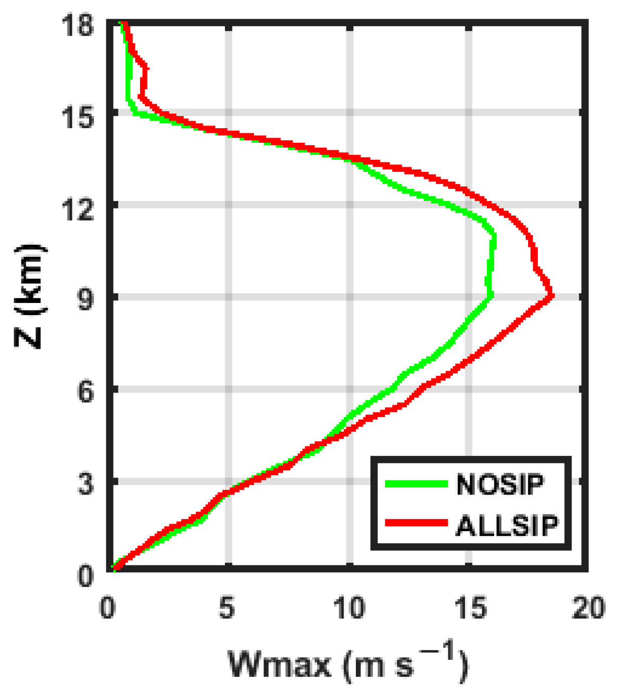
4.4. SIP-Related Microphysical Feedbacks in the Convective Region

Figure 16 shows the number concentration, mass concentration, and effective radius of snow, graupel, cloud water, and rainwater averaged in the convective region in the NOSIP and ALLSIP cases. The ALLSIP case generally has more ice-phase content and less liquid-phase content than the NOSIP case, indicating that SIPs accelerate cloud glaciation. In the mixed-phase layer (5 to 11 km), snow and graupel, respectively, have a 358% and 36% increase in the vertically averaged number concentration in the ALLSIP case, compared with the NOSIP case. Snow also has a 51% increase in mass concentration, but graupel has a 13% decrease in mass concentration. Cloud water and rainwater, respectively, decrease by 41% and 40% in mass concentration. In the anvil layer (above 11 km), the number and mass concentrations of snow and graupel change little. In the warm layer (below 5 km), the number concentration of rainwater is increased by 10%, while the number concentration of cloud water is fixed in this study and not shown in the figure. The masses of rainwater and cloud water decreased by 5% and 16%, respectively. In addition, the effective radius of all the particle types has decreased, indicating the important role of SIPs in affecting particle sizes. SIPs mainly occur and have a strong influence on the microphysical properties in the mixed-phase layer. In the following, we mainly focus on the SIP-related microphysical feedbacks in the mixed-phase layer. The subsequent influences on the anvil layer and the warm layer in the convective region will also be discussed.

In the mixed-phase layer of the convective region, the increased ice crystal number from SIPs leads to increased snow number primarily through the enhanced autoconversion of ice crystals, as shown in Figure 17a. SIPs also lead to a significant increase in the rate of ice-rain collisions, which plays a secondary role in snow number production. Meanwhile, enhanced ice-rain collision becomes the dominant process that leads to a graupel number increase in the ALLSIP case, whereas nucleation of rain and snow-rain collision are the dominant processes in the NOSIP case (Figure 17c). The increased number of ice crystals and snow leads to significantly enhanced depositional growth, which is the primary reason for the increased mass of ice crystals and snow in the ALLSIP case. The depositional growth rate of ice crystals increases from 10⁻⁵ g m⁻² s⁻¹ in the NOSIP case to 10⁻³ g m⁻² s⁻¹ in the ALLSIP case, meanwhile, the depositional growth rate of snow increases from 0.7 g m⁻² s⁻¹ in the NOSIP case to 2.1 g m⁻² s⁻¹ in the ALLSIP case (Figure 17b). The enhanced depositional growth consumes a large amount of liquid water, and thus the riming rates of snow and graupel both decrease (Figure 17b,d). Therefore, the contribution of riming to snow mass is less important, whereas the contribution of depositional growth is more important and becomes the primary reason for snow mass increase in the ALLSIP case. The weaker riming of the graupel is the dominant reason for the graupel mass decrease in the ALLSIP case.

In the anvil layer, SIPs do not cause direct feedback but can affect PIPs by influencing the liquid water amount transported aloft from the mixed-phase layer. Less liquid water leads to a decreased homogeneous nucleation rate in the anvil layer (Figure 15b), meanwhile, the smaller liquid droplets aloft also lead to smaller ice crystals with lower fall velocity in the anvil layer (Figure 13c). The increase in ice crystals due to lower fall velocity offsets the decrease in ice production from a slower homogeneous nucleation rate, resulting in a small increase in ice crystal number, as seen in Figure 13a. The deposition of ice crystals is weak, and hence the mass of ice crystals is increased slightly. The slightly increased number of snow and graupel is caused by the slightly enhanced autoconversion of ice crystals and ice-rain collisions, as well as by lower fall velocity due to smaller sizes (see Figure 16). More numerous but smaller snow and graupel particles make their mass change insignificant.

The microphysical properties of the warm layer in the convective region are also affected by the SIP-related microphysical feedbacks in the mixed-phase layer. In the warm layer, the rain number is increased in the ALLSIP case mainly due to the melting of more numerous snow particles (Figure 17e). But the melting of snow does not directly contribute much to the rain mass, because of the smaller snow size in the ALLSIP case. Rain mass is decreased mainly due to the weaker warm rain process (Figure 17f). The warm rain process becomes weaker because of two factors. One is smaller rain from the melting of smaller snow and graupel. The other is the decreased cloud water mass.

The microphysical feedbacks in the mixed-phase layer caused by SIPs could in turn affect the SIPs. It is found that the riming rate of snow and graupel are both decreased in the ALLSIP case. Therefore, rime splintering becomes weaker because the parameterization of rime splintering depends on the mass of rimed liquid produced by snow and graupel. Moreover, the vertically-integrated rate of rime splintering averaged in the convective region is 6.6 × 10⁴ m⁻² s⁻¹ in the ALLSIP case (with three SIPs), and 8.7 × 10⁴ m⁻² s⁻¹ in the RS case (only with rime splintering). This indicates that rime splintering is negative feedback. Freezing drop shattering is also a negative feedback because the rain droplets are decreased in cases with SIPs. Moreover, freezing drop shattering has a negligible effect on ice multiplication due to the limited number of large droplets. In addition, SIPs lead to more numerous but smaller snow and graupel. The increased number concentrations of snow and graupel lead to an increased collision rate, whereas smaller snow and graupel can lead to a smaller collision rate. Note that, whether it is positive or negative feedback, all SIPs lead to ice multiplication, but to different degrees. Ice-ice collisional breakup has the highest contribution to ice production in this squall line case.

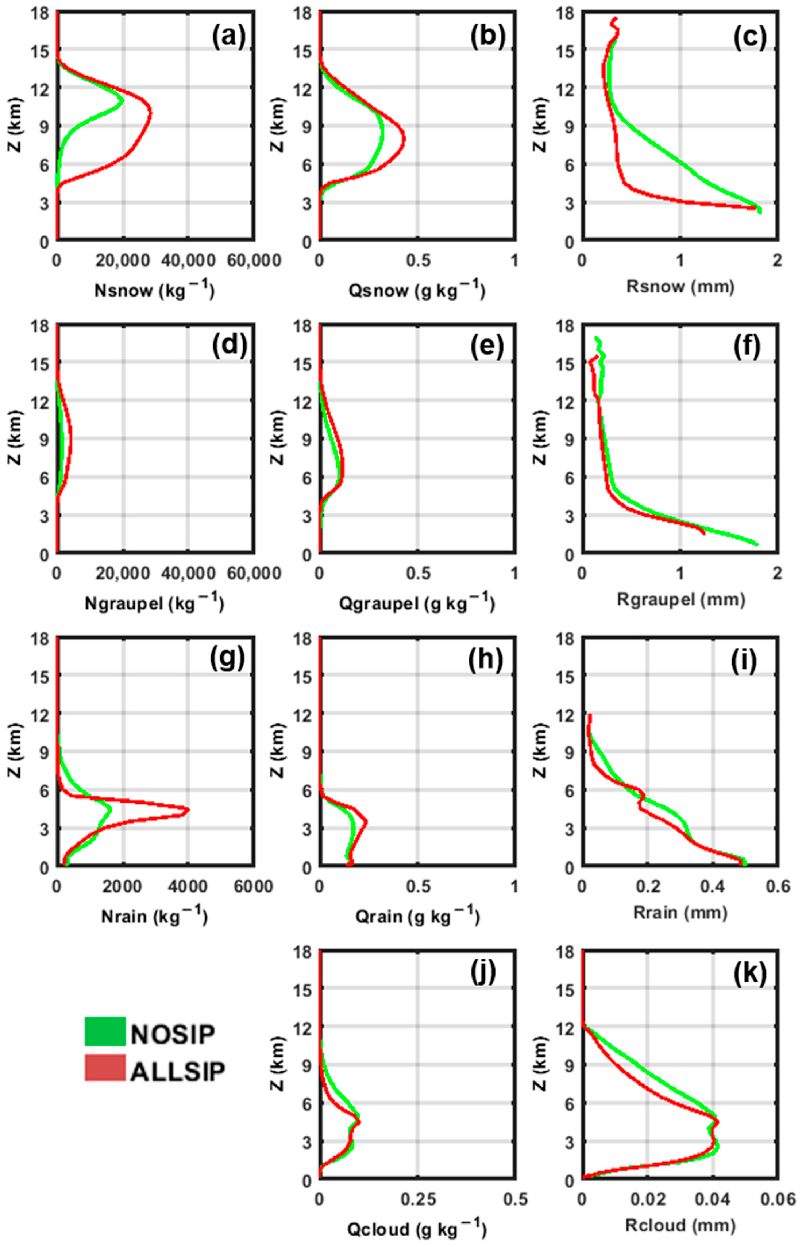
4.5. SIP-Related Microphysical Feedbacks in the Stratiform Region

Figure 18 shows the number concentration, mass concentration, and effective radius of snow, graupel, cloud water, and rainwater averaged in the stratiform region in the NOSIP and ALLSIP cases. In the mixed-phase layer and anvil layer, the main hydrometeor is snow, in addition to ice crystals. Snow number and mass increased by 230% and 26%, respectively, in the ALLSIP case in the mixed-phase layer, while they increased by 26% and 26% in the anvil layer. Graupel and supercooled water both have little amount in the mixed-phase and anvil layers and change little by the SIPs. In the warm layer, rain and cloud water have similar amounts. The rainwater number increases by 44% in the ALLSIP case, while the cloud water number is fixed. Rain mass increases by 28%, but cloud water mass has no significant change. In addition, the effective radius of snow and rain decreases, while that of graupel and cloud water changes little. In the following, we analyze the SIP-related microphysical feedbacks in the stratiform region and mainly focus on the changes in snow and rain.

In the mixed-phase layer, where SIPs mainly occur, the microphysical reasons for the increased snow number and mass are the enhanced local autoconversion of ice crystal process and deposition of snow, respectively (Figure 19a,b), similar to the convective region. The processes leading to the increase in snow number and mass in the anvil layer are also the autoconversion of ice crystals and the deposition of snow, respectively. Previous studies show that the microphysical properties of the stratiform region are determined by a combination of transport from the convective region and local microphysical processes [68,73,74]. As can be seen from Figure 11a,d, there are air flows from the upper levels of the convective region to the stratiform region, implying the transport of hydrometeors from the convective region to the stratiform region. Therefore, the increased number and mass concentration of snow in the stratiform region may also be caused by the increased transport from the convective region, where snow number and mass are higher. However, this study does not aim to investigate the relative importance of transport and local microphysics. Our focus is on the effect of SIPs on microphysical properties.

In the warm layer of the stratiform region, the increased rain number and mass are mainly due to the increased melting of snow directly (Figure 19c,d), which is the dominant process among rainwater production. The rain mass is increased also through the enhanced melting of graupel and warm rain processes, but these two processes are not the dominant causes. In addition, the melting of snow occurs in a wide range of stratiform regions, while the melting of graupel and warm rain processes only occur in the limited stratiform region close to the convective region. This is most likely because the formation and growth of graupel is mainly limited to the convective region, whereas the formation and growth of snow can spread over both the convective and stratiform regions.

The stratiform region has limited supercooled water in the mixed-phase layer, and therefore the feedbacks involving deposition and riming as in the convective region have relatively small effects. In addition, the ice multiplication is weaker in the stratiform region than in the convective region (as can be seen in Figure 13).

5. Discussion

This study is focused on the mature stage of a midlatitude continental MCS. The SIP-related microphysical feedback is very important at this stage. However, a detailed analysis of the SIPs in the early stages is not included in this study. It is possible that different SIPs work at different stages of the same cloud. Qu et al. [32] found that, in a tropical maritime deep convective cloud, freezing drop shattering contributes most to the ice multiplication during the developing stage of cloud evolution, while ice-ice collisional breakup dominates when clouds become nearly glaciated. Rime splintering is not important in this case. Consistently, this study found that ice-ice collisional breakup dominates in the mature stage of a midlatitude continental MCS. Given that this MCS is embedded in a cold frontal cloud during its initial stage, another MCS case or an ideal case may be more suitable to explore which SIP is dominant and whether these microphysical feedbacks exist in the initial stage of a midlatitude continental MCS.

Freezing drop shattering is not important in this case because supercooled liquid water is only sufficient in limited areas of the cloud in the mature stage. This is quite different from cumulus congestus in tropical regions (e.g., [21]) and tropical MCSs [33], where supercooled liquid water is the dominant phase and freezing drop shattering is very important. In contrast to tropical maritime clouds, measurements in midlatitude continental clouds show that updraft cores do not develop large (≥70 μm) supercooled drops [30,39]. Less LWC and fewer large drops in this midlatitude continental MCS may result in a small role of freezing drop shattering. Future studies could investigate if a limited number of large drops is the main reason for freezing drop shattering to be unimportant.

The SIP-related microphysical feedback described in the mature stage of this squall line case is different from the feedback in Arctic stratocumulus clouds. Here, the microphysical feedbacks associated with ice-ice collisional breakup weaken rime splintering. This study also found that rime splintering has little effect on ice-ice collisional breakup because the rates of ice-ice collisional breakup in the ALLSIP case and CB case have little difference. However, in the Arctic stratocumulus cloud, rime splintering can enhance ice-ice collisional breakup, and ice-ice collisional breakup is weak when activated alone [47]. The different feedbacks may be caused by different water contents in different clouds. The ice water content of MCSs is sufficient to initiate ice-ice collisional breakup at a high rate, and there is also sufficient liquid water content to maintain a high rate of ice-ice collisional breakup by allowing secondary ice crystals to grow into snow and graupel through deposition. However, Arctic clouds have very few ice-phase particles and liquid-phase particles, so rime splintering is needed to generate more ice-phase particles to maintain the high collisional breakup rate.

This study found that including SIPs (mainly ice-ice collisional breakup) results in an increase of about 27% in the ice number concentration and a decrease of 19% in the radius of ice particles in the anvil layer. This kind of change in cloud microphysical properties is similar to the aerosol effect on anvil clouds, which may result in a significant change in cloud radiative properties [75]. The simulations without ice-ice collisional breakup process in Fan et al. [75] show that the ice crystal number concentration in the anvil layer increases by a factor of 3–5 and the size of ice particles is reduced by up to 50% when the initial aerosol concentrations increase by a factor of 6. It seems that SIPs and increased aerosol number concentrations have similar effects on the anvil layer, but the aerosol effect is stronger than the SIP effect. The relative importance and joint impact of SIPs and aerosol effects on cloud anvils can be studied in the future.

The study of Han et al. [68] mentioned that the simulated precipitation rate in the stratiform region of squall lines is often lower, while that in the convective region is often higher than the observation, but the reason is still unclear. Several mechanisms, including SIPs, have been proposed, but ice-ice collisional breakup is not considered in their study. Our study shows that adding ice-ice collisional breakup can lead to less precipitation in the convective region and more precipitation in the stratiform region. Moreover, including three SIPs (especially ice-ice collisional breakup) improves the simulations of the convective area and precipitation rate in the convective region. Note that the parameterizations of three SIPs utilized in the study are based on theoretical results or laboratory results. The ALLSIP case that uses these parameterizations has a better simulation of the surface precipitation and radar reflectivity for this squall line. In the future, more model simulations for more cases are needed to investigate if considering SIPs can improve the simulations in other clouds.

The microphysical feedback in the convective region caused by SIPs could change the latent heats, which could have an impact on the dynamics. As can be seen from Figure 20, the maximum vertical velocity in the convective region increases in the mixed-phase layer in the ALLSIP case. The stronger updrafts may be caused by the SIP-induced phase transition from water vapor and liquid to ice phase, which promotes latent heat release and convection invigoration. However, surface precipitation still decreases as the cloud is invigorated, possibly because the microphysical feedbacks are strong and can dominate over the dynamic effects.

6. Conclusions

Three SIPs, including rime splintering, freezing drop shattering, and ice-ice collisional breakup, were investigated in a squall line case in North China on 18 August 2020 using the WRF model with the Morrison double-moment bulk microphysical scheme, which originally includes rime splintering. Freezing drop shattering and ice-ice collisional breakup processes are added to the Morrison scheme here. This study mainly investigates the relative importance of rime splintering, freezing drop shattering, and ice-ice collisional breakup in the mature stage of the squall line case.

The simulations show that including SIPs in the model, especially ice-ice collisional breakup, improves the simulations of convective area and convective precipitation rate, but slightly improves the simulations in the stratiform region. SIPs mainly occur in the mixed-phase layer, exhibiting the most pronounced effect on ice production at about the −8 °C (~6 km) level. Here, ice-ice collisional breakup and rime splintering can respectively increase ice crystal number concentration by up to 5 and 4 orders of magnitude compared to the simulation with no SIPs. Freezing drop shattering has a negligible effect on ice production because there are few large droplets in the mature stage. Ice-ice collisional breakup affects both the convective and stratiform regions of the squall line case, while rime splintering mainly affects the convective region but occurs in a limited area in the stratiform region.

A chain of microphysical changes occurs in the convective region and stratiform region. Following the ice multiplication by ice-ice collisional breakup and rime splintering, autoconversion of ice crystals and ice-rain collision are enhanced, leading to more numerous snow and graupel. The increased number of ice-phase particles enhances the deposition process, which increases the mass of ice and snow while decreasing the mass of supercooled water through WBF. Subsequently, this weakens the riming process and decreases the mass of the graupel. Notably, all the ice-phase particles have a smaller size in the ALLSIP case compared to the NOSIP case.

Moreover, this chain of microphysical changes can feedback to rime splintering and ice-ice collisional breakup in different ways. Rime splintering is limited by itself and also limited by ice-ice collisional breakup because the weaker riming due to the two SIPs leads to a lower rime splintering rate, as set in the parameterization of rime splintering. Therefore, in the presence of ice-ice collisional breakup, rime splintering plays a secondary role in secondary ice production in the mature stage of the system. In addition, SIPs lead to more numerous but smaller snow and graupel. The increased number concentrations of snow and graupel lead to an increased collision rate, whereas smaller snow and graupel can lead to a smaller collision rate. Note that, whether it is positive or negative feedback, all SIPs lead to ice multiplication, but to different degrees. The ice-ice collisional breakup has the highest contribution to ice production in this squall line case.

The ice-ice collisional breakup has a slower rate than the primary ice production in the anvil layer. Therefore, it does not directly affect ice production in the anvil layer. However, ice-ice collisional breakup can affect PIPs by transporting fewer and smaller droplets aloft from the mixed-phase layer in the convective region. The fewer droplets and smaller droplets lead to fewer and smaller ice crystals through PIPs, which have a lower fall velocity. The lower fall velocity of smaller ice crystals leads to an increase in ice number, offsetting the decrease in ice production from PIPs, resulting in an increase of 27% and 7% in ice crystal number and mass in the convective region, respectively. The stratiform region has increased in ice number and mass, which is also due to the transport of ice from the convective to the stratiform region.

The rainwater in the warm layer and the surface precipitation rates are also affected by ice-ice collisional breakup. In the convective region, warm rain is the dominant process for rain mass. Ice-ice collisional breakup, on the one hand, can lead to more numerous and smaller snow in the mixed-phase layer, resulting in more and smaller raindrops after melting. On the other hand, ice-ice collisional breakup can lead to decreased cloud water mass through enhanced WBF. Therefore, the warm rain process becomes weaker, and the rain mass decreases. In the stratiform region, the melting of snow is the dominant process for rain mass. Ice-ice collisional breakup increases snow number and mass, and the enhanced melting of snow directly leads to increased number and mass concentrations of rain in the warm layer. As such, there is a smaller surface precipitation rate in the convective region and a larger rate in the stratiform region. Compared with observations, including SIPs (especially ice-ice collisional breakup) in the model improves the simulations of convective area and convective precipitation rate, but slightly improves the simulations in the stratiform region.

This study only simulated one midlatitude continental squall line case. In the future, it is necessary to consider whether the roles of the three SIPs are different among different MCSs. In addition, the relative importance and joint impact of SIPs and aerosol effects on cloud anvils can be studied in the future.

References

1. Clark, P.D.; Choularton, T.W.; Brown, P.R.A.; Field, P.R.; Illingworth, A.J.; Hogan, R.J. Numerical modelling of mixed-phase frontal clouds observed during the CWVC project. Q. J. R. Meteorol. Soc. 2005, 131, 1677–1693. [Google Scholar] [CrossRef]
2. Crosier, J.; Choularton, T.W.; Westbrook, C.D.; Blyth, A.M.; Bower, K.N.; Connolly, P.J.; Dearden, C.; Gallagher, M.W.; Cui, Z.; Nicol, J.C. Microphysical Properties of Cold Frontal Rainbands. Q. J. R. Meteorol. Soc. 2013, 140, 1257–1268. [Google Scholar] [CrossRef]
3. Field, P.R.; Lawson, R.P.; Brown, P.R.A.; Lloyd, G.; Westbrook, C.; Moisseev, D.; Miltenberger, A.; Nenes, A.; Blyth, A.; Choularton, T.; et al. Chapter 7. Secondary Ice Production-current state of the science and recommendations for the future. Meteorol. Monogr. 2017, 58, 7.1–7.20. [Google Scholar] [CrossRef]
4. Finlon, J.A.; Rauber, R.M.; Wu, W.; Zaremba, T.J.; McFarquhar, G.M.; Nesbitt, S.W.; Schnaiter, M.; Järvinen, E.; Waitz, F.; Hill, T.C.J.; et al. Structure of an Atmospheric River Over Australia and the Southern Ocean: II. Microphysical Evolution. J. Geophys. Res. Atmos. 2020, 125, e2020JD032514. [Google Scholar] [CrossRef]
5. Hobbs, P.V.; Rangno, A.L. Ice Particle Concentrations in Clouds. J. Atmos. Sci. 1985, 42, 2523–2549. [Google Scholar] [CrossRef]
6. Ladino, L.A.; Korolev, A.; Heckman, I.; Wolde, M.; Fridlind, A.M.; Ackerman, A.S. On the role of ice-nucleating aerosol in the formation of ice particles in tropical mesoscale convective systems. Geophys. Res. Lett. 2017, 44, 1574–1582. [Google Scholar] [CrossRef] [PubMed]
7. Lasher-Trapp, S.; Leon, D.C.; DeMott, P.J.; Villanueva-Birriel, C.M.; Johnson, A.V.; Moser, D.H.; Tully, C.S.; Wu, W. A Multisensor Investigation of Rime Splintering in Tropical Maritime Cumuli. J. Atmos. Sci. 2016, 73, 2547–2564. [Google Scholar] [CrossRef]
8. Hallett, J.; Mossop, S.C. Production of Secondary Ice Particles During Riming Process. Nature 1974, 249, 26–28. [Google Scholar] [CrossRef]
9. Langham, E.J.; Mason, B.J. The heterogeneous and homogeneous nucleation of supercooled water. Proc. R. Soc. London. Ser. A Math. Phys. Sci. 1958, 247, 493–504. [Google Scholar]
10. Takahashi, T.; Nagao, Y.; Kushiyama, Y. Possible High Ice Particle Production during Graupel–Graupel Collisions. J. Atmos. Sci. 1995, 52, 4523–4527. [Google Scholar] [CrossRef]
11. Vardiman, L. The Generation of Secondary Ice Particles in Clouds by Crystal–Crystal Collision. J. Atmos. Sci. 1978, 35, 2168–2180. [Google Scholar] [CrossRef]
12. Bacon, N.J.; Swanson, B.D.; Baker, M.B.; Davis, E.J. Breakup of levitated frost particles. J. Geophys. Res. Atmos. 1998, 103, 13763–13775. [Google Scholar] [CrossRef]
13. Oraltay, R.; Hallett, J. Evaporation and melting of ice crystals: A laboratory study. Atmos. Res. 1989, 24, 169–189. [Google Scholar] [CrossRef]
14. Dye, J.E.; Hobbs, P.V. Influence of environmental parameters on freezing and fragmentation of suspended water drops. J. Atmos. Sci. 1968, 25, 82–96. [Google Scholar] [CrossRef]
15. King, W.D.; Fletcher, N.H. Thermal Shock as an Ice Multiplication Mechanism. Part I. Theory. J. Atmos. Sci. 1976, 33, 85–96. [Google Scholar] [CrossRef]
16. Baker, B.A. On the Nucleation of Ice in Highly Supersaturated Regions of Clouds. J. Atmos. Sci. 1991, 48, 1904–1907. [Google Scholar] [CrossRef]
17. Korolev, A.; Leisner, T. Review of experimental studies of secondary ice production. Atmos. Meas. Tech. 2020, 20, 11767–11797. [Google Scholar] [CrossRef]
18. Heymsfield, A.; Willis, P. Cloud Conditions Favoring Secondary Ice Particle Production in Tropical Maritime Convection. J. Atmos. Sci. 2014, 71, 4500–4526. [Google Scholar] [CrossRef]
19. Korolev, A.; Heckman, I.; Wolde, M.; Ackerman, A.S.; Fridlind, A.M.; Ladino, L.A.; Lawson, R.P.; Milbrandt, J.; Williams, E. A new look at the environmental conditions favorable to secondary ice production. Atmos. Meas. Tech. 2020, 20, 1391–1429. [Google Scholar] [CrossRef]
20. Phillips VTJBlyth, A.M.; Brown, P.R.A.; Choularton, T.W.; Latham, J. The glaciation of a cumulus cloud over New Mexico. Q. J. R. Meteorol. Soc. 2001, 127, 1513–1534. [Google Scholar] [CrossRef]
21. Lawson, R.P.; Woods, S.; Morrison, H. The Microphysics of Ice and Precipitation Development in Tropical Cumulus Clouds. J. Atmos. Sci. 2015, 72, 2429–2445. [Google Scholar] [CrossRef]
22. Phillips, V.T.J.; Patade, S.; Gutierrez, J.; Bansemer, A. Secondary Ice Production by Fragmentation of Freezing Drops: Formulation and Theory. J. Atmos. Sci. 2018, 75, 3031–3070. [Google Scholar] [CrossRef]
23. Hoarau, T.; Pinty, J.-P.; Barthe, C. A representation of the collisional ice break-up process in the two-moment microphysics LIMA v1.0 scheme of Meso-NH. Geosci. Model Dev. 2018, 11, 4269–4289. [Google Scholar] [CrossRef]
24. Phillips, V.T.J.; Yano, J.-I.; Khain, A. Ice Multiplication by Breakup in Ice–Ice Collisions. Part I: Theoretical Formulation. J. Atmos. Sci. 2017, 74, 1705–1719. [Google Scholar]
25. Sullivan, S.C.; Barthlott, C.; Crosier, J.; Zhukov, I.; Nenes, A.; Hoose, C. The effect of secondary ice production parameterization on the simulation of a cold frontal rainband. Atmos. Meas. Tech. 2018, 18, 16461–16480. [Google Scholar] [CrossRef]
26. Blyth, A.M.; Latham, J. Development of ice and precipitation in New Mexican summertime cumulus clouds. Q. J. R. Meteorol. Soc. 1993, 119, 91–120. [Google Scholar] [CrossRef]
27. Huang, Y.; Blyth, A.M.; Brown, P.R.A.; Choularton, T.W.; Connolly, P.; Gadian, A.M.; Jones, H.; Latham, J.; Cui, Z.; Carslaw, K. The development of ice in a cumulus cloud over southwest England. New J. Phys. 2008, 10, 105021. [Google Scholar] [CrossRef]
28. Lasher-Trapp, S.; Scott, E.L.; Järvinen, E.; Schnaiter, M.; Waitz, F.; DeMott, P.J.; McCluskey, C.S.; Hill, T.C.J. Observations and Modeling of Rime Splintering in Southern Ocean Cumuli. J. Geophys. Res. Atmos. 2021, 126, e2021JD035479. [Google Scholar] [CrossRef]
29. Crosier, J.; Bower, K.N.; Choularton, T.W.; Westbrook, C.D.; Connolly, P.J.; Cui, Z.Q.; Crawford, I.P.; Capes, G.L.; Coe, H.; Dorsey, J.R.; et al. Observations of ice multiplication in a weakly convective cell embedded in supercooled mid-level stratus. Atmos. Meas. Tech. 2011, 11, 257–273. [Google Scholar] [CrossRef]
30. Hogan, R.J.; Field, P.R.; Illingworth, A.J.; Cotton, R.J.; Choularton, T.W. Properties of embedded convection in warm-frontal mixed-phase cloud from aircraft and polarimetric radar. Q. J. R. Meteorol. Soc. 2002, 128, 451–476. [Google Scholar] [CrossRef]
31. Hou, T.; Lei, H.; He, Y.; Yang, J.; Zhao, Z.; Hu, Z. Aircraft Measurements of the Microphysical Properties of Stratiform Clouds with Embedded Convection. Adv. Atmos. Sci. 2021, 38, 966–982. [Google Scholar] [CrossRef]
32. Qu, Y.; Khain, A.; Vaughan, P.; Eyal, I.; Shpund, J.S.; Patade, S.; Chen, B. The Role of Ice Splintering on Microphysics of Deep Convective Clouds Forming Under Different Aerosol Conditions: Simulations Using the Model With Spectral Biwithcrophysics. J. Geophys. Res. Atmos. 2020, 125, e2019JD031312. [Google Scholar] [CrossRef]
33. Qu, Z.; Korolev, A.; Milbrandt, J.A.; Heckman, I.; Huang, Y.; McFarquhar, G.M.; Morrison, H.; Wolde, M.; Nguyen, C. The impacts of secondary ice production on microphysics and dynamics in tropical convection. Atmos. Meas. Tech. 2022, 22, 12287–12310. [Google Scholar] [CrossRef]
34. Aleksić, N.M.; Farley, R.; Orville, H. A numerical cloud model study of the Hallett-Mossop ice multiplication process in strong convection. Atmos. Res. 1989, 23, 1–30. [Google Scholar] [CrossRef]
35. Phillips, V.T.J.; Choularton, T.W.; Blyth, A.M.; Latham, J. The influence of aerosol concentrations on the glaciation and precipitation of a cumulus cloud. Q. J. R. Meteorol. Soc. 2002, 128, 951–971. [Google Scholar] [CrossRef]
36. Keinert, A.; Spannagel, D.; Leisner, T.; Kiselev, A. Secondary Ice Production upon Freezing of Freely Falling Drizzle Droplets. J. Atmos. Sci. 2020, 77, 2959–2967. [Google Scholar] [CrossRef]
37. Lauber, A.; Kiselev, A.; Pander, T.; Handmann, P.; Leisner, T. Secondary Ice Formation during Freezing of Levitated Droplets. J. Atmos. Sci. 2018, 75, 2815–2826. [Google Scholar] [CrossRef]
38. Wildeman, S.; Sterl, S.; Sun, C.; Lohse, D. Fast Dynamics of Water Droplets Freezing from the Outside In. Phys. Rev. Lett. 2017, 118, 084101. [Google Scholar] [CrossRef]
39. Lawson, R.P.; Gurganus, C.; Woods, S.; Bruintjes, R. Aircraft Observations of Cumulus Microphysics Ranging from the Tropics to Midlatitudes: Implications for a “New” Secondary Ice Process. J. Atmos. Sci. 2017, 74, 2899–2920. [Google Scholar] [CrossRef]
40. Rangno, A.L. Fragmentation of Freezing Drops in Shallow Maritime Frontal Clouds. J. Atmos. Sci. 2008, 65, 1455–1466. [Google Scholar] [CrossRef]
41. Schwarzenboeck, A.; Shcherbakov, V.; Lefevre, R.; Gayet, J.-F.; Pointin, Y.; Duroure, C. Indications for stellar-crystal fragmentation in Arctic clouds. Atmos. Res. 2009, 92, 220–228. [Google Scholar] [CrossRef]
42. Phillips, V.T.J.; Yano, J.-I.; Formenton, M.; Ilotoviz, E.; Kanawade, V.; Kudzotsa, I.; Sun, J.; Bansemer, A.; Detwiler, A.G.; Kahin, A.; et al. Ice Multiplication by Breakup in Ice–Ice Collisions. Part II: Numerical Simulations. J. Atmos. Sci. 2017, 74, 2789–2811. [Google Scholar]
43. Dedekind, Z.; Lauber, A.; Ferrachat, S.; Lohmann, U. Sensitivity of precipitation formation to secondary ice production in winter orographic mixed-phase clouds. Atmos. Meas. Tech. 2021, 21, 15115–15134. [Google Scholar] [CrossRef]
44. Georgakaki, P.; Sotiropoulou, G.; Vignon, É.; Billault-Roux, A.-C.; Berne, A.; Nenes, A. Secondary ice production processes in wintertime alpine mixed-phase clouds. Atmos. Meas. Tech. 2022, 22, 1965–1988. [Google Scholar] [CrossRef]
45. Sotiropoulou, G.; Vignon, É.; Young, G.; Morrison, H.; O’Shea, S.J.; Lachlan-Cope, T.; Berne, A.; Nenes, A. Secondary ice production in summer clouds over the Antarctic coast: An underappreciated process in atmospheric models. Atmos. Meas. Tech. 2021, 21, 755–771. [Google Scholar] [CrossRef]
46. Morrison, H.; Curry, J.A.; Khvorostyanov, V.I. A New Double-Moment Microphysics Parameterization for Application in Cloud and Climate Models. Part I: Description. J. Atmos. Sci. 2005, 62, 1665–1677. [Google Scholar] [CrossRef]
47. Sotiropoulou, G.; Sullivan, S.; Savre, J.; Lloyd, G.; Lachlan-Cope, T.; Ekman, A.M.L.; Nenes, A. The impact of secondary ice production on Arctic stratocumulus. Atmospheric Meas. Tech. 2020, 20, 1301–1316. [Google Scholar] [CrossRef]
48. Sullivan, S.C.; Hoose, C.; Kiselev, A.; Leisner, T.; Nenes, A. Initiation of secondary ice production in clouds. Atmos. Meas. Tech. 2018, 18, 1593–1610. [Google Scholar] [CrossRef]
49. Connolly, P.J.; Choularton, T.W.; Gallagher, M.; Bower, K.N. Cloud-resolving simulations of intense tropicalHector thunderstorms: Implications for aerosol–cloud interactions. Q. J. R. Meteorol. Soc. 2006, 132, 3079–3106. [Google Scholar] [CrossRef]
50. Crawford, I.; Bower, K.N.; Choularton, T.W.; Dearden, C.; Crosier, J.; Westbrook, C.; Capes, G.; Coe, H.; Connolly, P.J.; Dorsey, J.R.; et al. Ice formation and development in aged, wintertime cumulus over the UK: Observations and modelling. Atmos. Meas. Tech. 2012, 12, 4963–4985. [Google Scholar] [CrossRef]
51. Huffman, G.J.; Bolvin, D.T.; Nelkin, E.J.; Wolff, D.B.; Adler, R.F.; Gu, G.; Hong, Y.; Bowman, K.P.; Stocker, E.F. The TRMM Multisatellite Precipitation Analysis (TMPA): Quasi-Global, Multiyear, Combined-Sensor Precipitation Estimates at Fine Scales. J. Hydrometeorol. 2007, 8, 38–55. [Google Scholar] [CrossRef]
52. Tian, Y.; Peters-Lidard, C.D.; Choudhury, B.J.; Garcia, M. Multitemporal Analysis of TRMM-Based Satellite Precipitation Products for Land Data Assimilation Applications. J. Hydrometeorol. 2007, 8, 1165–1183. [Google Scholar] [CrossRef]
53. Joyce, R.J.; Janowiak, J.E.; Arkin, P.A.; Xie, P. CMORPH: A Method that Produces Global Precipitation Estimates from Passive Microwave and Infrared Data at High Spatial and Temporal Resolution. J. Hydrometeorol. 2004, 5, 487–503. [Google Scholar] [CrossRef]
54. Jiang, L.; Bauer-Gottwein, P. How do GPM IMERG precipitation estimates perform as hydrological model forcing? Evaluation for 300 catchments across Mainland China. J. Hydrol. 2019, 572, 486–500. [Google Scholar] [CrossRef]
55. Skamarock, W.C.; Klemp, J.B.; Dudhia, J.; Gill, D.O.; Liu, Z.; Berner, J.; Wang, W.; Powers, J.G.; Duda, M.G.; Barker, D.M.; et al. A Description of the Advanced Research WRF Version 4; NCAR Tech; Note NCAR/TN-556+STR; National Center for Atmospheric Research: Boulder, CO, USA, 2019; 145p. [Google Scholar]
56. Morrison, H.; Thompson, G.; Tatarskii, V. Impact of Cloud Microphysics on the Development of Trailing Stratiform Precipitation in a Simulated Squall Line: Comparison of One- and Two-Moment Schemes. Mon. Weather. Rev. 2009, 137, 991–1007. [Google Scholar] [CrossRef]
57. Hong, S.-Y.; Noh, Y.; Dudhia, J. A New Vertical Diffusion Package with an Explicit Treatment of Entrainment Processes. Mon. Weather Rev. 2006, 134, 2318–2341. [Google Scholar] [CrossRef]
58. Mlawer, E.J.; Taubman, S.J.; Brown, P.D.; Iacono, M.J.; Clough, S.A. Radiative transfer for inhomogeneous atmospheres: RRTM, a validated correlated-k model for the longwave. J. Geophys. Res. Atmos. 1997, 102, 16663–16682. [Google Scholar] [CrossRef]
59. Dudhia, J. Numerical Study of Convection Observed during the Winter Monsoon Experiment Using a Mesoscale Two-Dimensional Model. J. Atmos. Sci. 1989, 46, 3077–3107. [Google Scholar] [CrossRef]
60. Kain, J.S. The Kain–Fritsch Convective Parameterization: An Update. J. Appl. Meteorol. 2004, 43, 170–181. [Google Scholar] [CrossRef]
61. Passarelli, R.E. An Approximate Analytical Model of the Vapor Deposition and Aggregation Growth of Snowflakes. J. Atmos. Sci. 1978, 35, 118–124. [Google Scholar] [CrossRef]
62. Verlinde, J.; Flatau, P.J.; Cotton, W.R. Analytical Solutions to the Collection Growth Equation: Comparison with Approximate Methods and Application to Cloud Microphysics Parameterization Schemes. J. Atmos. Sci. 1990, 47, 2871–2880. [Google Scholar] [CrossRef]
63. Ikawa, M.; Saito, K. Description of a nonhydrostatic model developed at the forecast research department of the MRI. Meteorol. Res. Institude Tech. Rep. 1991, 28, 238. [Google Scholar]
64. Reisner, J.; Rasmussen, R.M.; Bruintjes, R.T. Explicit forecasting of supercooled liquid water in winter storms using the MM5 mesoscale model. Q. J. R. Meteorol. Soc. 1998, 124, 1071–1107. [Google Scholar] [CrossRef]
65. Churchill, D.D.; Houze, R.A., Jr. Development and Structure of Winter Monsoon Cloud Clusters On 10 December 1978. J. Atmos. Sci. 1984, 41, 933–960. [Google Scholar] [CrossRef]
66. Fan, J.; Han, B.; Varble, A.; Morrison, H.; North, K.; Kollias, P.; Chen, B.; Dong, X.; Giangrande, S.E.; Khain, A.; et al. Cloud-resolving model intercomparison of an MC3E squall line case: Part I—Convective updrafts. J. Geophys. Res. Atmos. 2017, 122, 9351–9378. [Google Scholar] [CrossRef]
67. Liu, Y.-C.; Fan, J.; Zhang, G.J.; Xu, K.-M.; Ghan, S.J. Improving representation of convective transport for scale-aware parameterization: 2. Analysis of cloud-resolving model simulations. J. Geophys. Res. Atmos. 2015, 120, 3510–3532. [Google Scholar] [CrossRef]
68. Han, B.; Fan, J.; Varble, A. Cloud-Resolving Model Intercomparison of an MC3E Squall Line Case: Part II. Stratiform Precipitation Properties. J. Geophys. Res. Atmos. 2019, 124, 1090–1117. [Google Scholar] [CrossRef]
69. Shpund, J.; Khain, A.; Lynn, B.; Fan, J.; Han, B.; Ryzhkov, A.; Snyder, J.; Dudhia, J.; Gill, D. Simulating a Mesoscale Convective System Using WRF With a New Spectral Bin Microphysics: 1: Hail vs Graupel. J. Geophys. Res. Atmos. 2019, 124, 14072–14101. [Google Scholar] [CrossRef]
70. Shahi, N.K.; Polcher, J.; Bastin, S.; Pennel, R.; Fita, L. Assessment of the spatio-temporal variability of the added value on precipitation of convection-permitting simulation over the Iberian Peninsula using the RegIPSL regional earth system model. Clim. Dyn. 2022, 59, 471–498. [Google Scholar] [CrossRef]
71. Stoelinga, M.T. Simulated Equivalent Reflectivity Factor as Currently Formulated in RIP: Description and Possible Improvements. White Paper, 2005; 5p. [Google Scholar]
72. Korolev, A. Limitations of the Wegener–Bergeron–Findeisen Mechanism in the Evolution of Mixed-Phase Clouds. J. Atmos. Sci. 2007, 64, 3372–3375. [Google Scholar] [CrossRef]
73. Varble, A.; Zipser, E.J.; Fridlind, A.M.; Zhu, P.; Ackerman, A.S.; Chaboureau, J.P.; Collis, S.; Fan, J.; Hill, A.; Shipway, B. Evaluation of cloud-resolving and limited area model intercomparison simulations using TWP-ICE observations: 1. Deep convective updraft properties. J. Geophys. Res. Atmos. 2014, 119, 13891–13918. [Google Scholar] [CrossRef]
74. Varble, A.; Zipser, E.J.; Fridlind, A.M.; Zhu, P. Evaluation of cloud-resolving and limited area model intercomparison simulations using TWP-ICE observations: 2. Precipitation microphysics. J. Geophys. Res. Atmos. 2014, 119, 13919–13945. [Google Scholar] [CrossRef]
75. Fan, J.; Leung, L.R.; Rosenfeld, D.; Chen, Q.; Li, Z.; Zhang, J.; Yan, H. Microphysical effects determine macrophysical response for aerosol impacts on deep convective clouds. Proc. Natl. Acad. Sci. USA 2013, 110, E4581–E4590. [Google Scholar] [CrossRef] [PubMed]
Figure 1. Skew T-logP diagram based on profiles averaged in the region between 37° N–43° N and 115° E–123° E at 14:00 BJT on 18 August 2020 (06:00 UTC on 17 August 2020) according to the FNL analysis.
Atmosphere 14 01752 g001
Figure 2. The visible image from Himawari-8 at 15:00 BJT on 18 August 2020 and the domain design of the WRF model. Domains 1 and 2 are abbreviated to d01 and d02, respectively.
Atmosphere 14 01752 g002
Figure 3. The distribution of weight function w R S in the rime splintering (a) and shattering probability p D S in the freezing droplet shattering (b).
Atmosphere 14 01752 g003aAtmosphere 14 01752 g003b
Figure 4. Spatial distribution of precipitation rate for GPM (left column), NOSIP case (middle column), and ALLSIP case (right column) for the 10 snapshots from 10:00 to 19:00 BJT. Only precipitation rates higher than 0.01 mm h−1 are plotted in this figure.
Atmosphere 14 01752 g004aAtmosphere 14 01752 g004b
Figure 5. (ac) The time series of convective area (a), area-average precipitation rate (b), and area-integrated precipitation rate (c) for the convective region. (df) The same as in (ac), but for the stratiform region. (gi) The temporal average of area, the area-average precipitation rate, and the area-integrated precipitation rate of the convective and stratiform regions, respectively. The convective and stratiform regions are defined by a threshold of 15 mm h−1.
Atmosphere 14 01752 g005
Figure 6. (a) Histogram of the precipitation area of each bin. (b) Histogram of the difference in area-average precipitation rate in each bin between the simulated case and the GPM observation. (c) Histogram of the area-integrated precipitation rate in each bin. The analysis time period is 14:00–19:00 BJT.
Atmosphere 14 01752 g006aAtmosphere 14 01752 g006b
Figure 7. Spatial distribution of composite radar reflectivity (unit: dBZ) for observations (left column), NOSIP case (middle column), and ALLSIP case (right column) for the 10 snapshots from 10:00 to 19:00 BJT. The composite radar reflectivity is calculated as the maximum radar reflectivity in each column. The color bar used for composite radar reflectivity is exactly the same for observations and simulations.
Atmosphere 14 01752 g007aAtmosphere 14 01752 g007b
Figure 8. The histogram of the composite radar reflectivity. The analysis time period is 14:00–19:00 BJT for the observation, NOSIP case, and ALLSIP case. The studied area in the NOSIP and ALLSIP cases is 37° N–43° N and 115° E–123° E. The studied area in the observation is shown in the left column of Figure 7. The fraction is the ratio of the area of each bin to the total area of the studied region.
Atmosphere 14 01752 g008
Figure 9. The time series of the fraction of area with the radar reflectivity larger than 30 dBZ (a), 40 dBZ (b), and 50 dBZ (c). The fraction is the ratio of the area for each bin to the total area of the studied region.
Atmosphere 14 01752 g009
Figure 10. The temporal average of precipitation area (a), temporal and area-average precipitation rate (b), and temporal average of area-integrated precipitation rate (c) of the convective and stratiform region for the GPM observation, 6 ensembles of the NOSIP case, and 6 ensembles of the ALLSIP case. The analysis time range is 14:00–19:00 BJT. Color bars are the means of the ensembles, and the error bar represents the maximum and minimum value in the 6 ensemble simulations.
Atmosphere 14 01752 g010
Figure 11. (a) The time-averaged vertical cross-section of radar reflectivity (shading, unit: dbz), wind (arrows), and temperature (red line, unit: °C) in the NOSIP case. (b) The time-averaged vertical cross-section of snow mass (shading, unit: g kg−1), graupel mass (black line, unit: g kg−1), and ice crystal mass (green line, unit: g kg−1) in the NOSIP case. (c) The time-averaged vertical cross-section of rain water mass (shading, unit: g kg−1) and cloud water mass (black line, unit: g kg−1) in the NOSIP case. Panels (df) are the same as in panels (ac), but for the ALLSIP case. Note that the time-averaged vertical cross-section is calculated based on the relative distance to the leading edge of the storm for all 13 snapshots between 17:00 and 19:00 BJT.
Atmosphere 14 01752 g011
Figure 12. (a) The fraction of the grids belonging to the mixed-phase (with both liquid and ice phase particles) to all grids in each precipitation rate bin. (b) The fraction of the grids satisfying both the conditions of subsaturation for liquid water and supersaturation for ice in all grids in each precipitation rate bin. (c) The fraction of the grids where the WBF process could occur to all grids in each precipitation rate bin. Between the two solid gray lines is the mixed-phase layer (5–11 km). The gray dashed line represents the separation line between the convective region and the stratiform region. The analysis time range is 17:00–19:00 BJT.
Atmosphere 14 01752 g012
Figure 13. Vertical profile of the number concentration (a,d), mass concentration (b,e), and effective radius (c,f) of ice crystals averaged in the convective region (ac) and stratiform region (df) during 17:00 BJT to 19:00 BJT for five cases. The small boxes in these panels are the profiles of the 11–18 km (anvil layer) in a linear scale for the NOSIP case and the ALLSIP case.
Atmosphere 14 01752 g013
Figure 14. The distribution of vertically integrated rime splintering rate (a), freezing drop shattering rate (b), and total ice-ice collisional breakup rate (c) in the ALLSIP case at 17:00 BJT. The black line in (ac) represents the boundary of the convective region.
Atmosphere 14 01752 g014
Figure 15. The vertically integrated production rates of ice crystals averaged of the convective region (a,b) and stratiform region (c,d) during 17:00 BJT and 19:00 BJT for the ALLSIP case. (a,c) are for the mixed-phase layer. (b,d) are for the anvil layer. Note that GGCB, SGCB, IGCB, SSCB, and ISCB represent graupel-graupel, snow-graupel, ice crystal-graupel, snow-snow, and ice crystal-snow collisional breakup. RS represents rime splintering. DS represents freezing drop shattering. HE and HO represent heterogeneous nucleation and homogeneous nucleation.
Atmosphere 14 01752 g015
Figure 16. Vertical profile of the number concentration (a,d,g), mass concentration (b,e,h,j), and effective radius (c,f,i,k) of snow (ac), graupel (df), rain water (gi), and cloud water (j,k) averaged in the convective region during 17:00 BJT and 19:00 BJT for the NOSIP and ALLSIP cases.
Atmosphere 14 01752 g016
Figure 17. Simulated vertically integrated production rates of the number concentration (a,c,e) and mass concentration (b,d,f) of snow (a,b), graupel (c,d) and rainwater (e,f) averaged in the convective region during 17:00 BJT and 19:00 BJT. Note that the warm rain process includes the autoconversion of cloud droplets to raindrops and the collection of cloud droplets by raindrops.
Atmosphere 14 01752 g017
Figure 18. Vertical profile of the number concentration (a,d,g), mass concentration (b,e,h,j), and effective radius (c,f,i,k) of snow (ac), graupel (df), rain water (gi), and cloud water (j,k) averaged in the stratiform region during 16:00 BJT and 19:00 BJT for the NOSIP and ALLSIP cases.
Atmosphere 14 01752 g018
Figure 19. Simulated vertically integrated production rates of the number concentration (a,c,e) and mass concentration (b,d,f) of snow (a,b), graupel (c,d) and rainwater (e,f) averaged in the stratiform region during 17:00 BJT and 19:00 BJT.
Atmosphere 14 01752 g019
Figure 20. Vertical profiles of maximum vertical velocity in the convective region during 17:00 and 19:00 BJT.
Atmosphere 14 01752 g020