Variability in Global Climatic Circulation Indices and Its Relationship

Abstract

Global climatic circulation indices play a major role in determining regional and global climate conditions. These atmospheric circulation patterns exhibit substantial variability, covering a wide geographical area and affecting weather-related events. The primary goal of this study was to examine and characterize various global climatic variability indices during the 1950 to 2020 period (El Niño Southern Oscillation, ENSO; Southern Oscillation Index, SOI; North Atlantic Oscillation, NAO; Atlantic Meridional Mode, AMM; and Indian Ocean Dipole, IOD). Also, this article try to investigating the link between these global climatic indices. Trend analysis showed that the ENSO index exhibits the highest recurrence frequency of correlation relationships with the other yearly global indices with significance at the 95% and 99% levels, while the NAO index exhibits the lowest recurrence frequency. On a seasonal basis, most indices demonstrate more abrupt changes during the winter season than during the summer. An increase occurred in events of abrupt changes in these indices over the last two decades (2000 to 2020), especially annually and in summer. The SOI exhibits the largest number of abrupt changes throughout the entire study period, spanning from positive to negative significant trends, whereas the IOD did not exhibit abrupt changes annually. Increasing and decreasing trends in the global climatic circulation indices may be related to natural and anthropogenic causes of climate change. Regarding both the correlation coefficient (CC) and partial correlation results, there existed a highly negative association between the ENSO and SOI in the annual, winter and summer time series. On the other hand, there is no relationship between ENSO and NAO. Furthermore, on an annual basis, there existed a highly negative association between the NAO and AMM and a less negative but still statistically significant association between these indices during the winter and summer seasons, respectively. Therefore, through the Azore high, the NAO could promote AMM. Moreover, when the NAO, AMM, and SOI are held constant, a positive and robust correlation is reached between the ENSO and IOD in winter season. Therefore, a developing IOD is intensified and sustained during the onset of an El Niño event in winter season.

1. Introduction

The atmosphere is disturbed by oceanic heat sources, which allows waves to disperse as they return to their original state. These waves define teleconnection patterns by influencing the climate in remote areas [1]. According to the Intergovernmental Panel on Climate Change (IPCC), climate indices link nearby regions mainly through large-scale, quasistationary atmospheric Rossby waves, and as a result, certain regions receive more precipitation or are hotter than indicated by the prevailing global-scale changes [2]. In addition, climate variation occurs due to large-scale ocean and atmospheric circulations, moisture transportation and heat fluxes. Changes in the natural patterns of the modes of atmospheric and oceanic variability control global weather and climate variations on seasonal, annual, or longer time scales, and any change in the behavior or relationships among these climate modes can lead to changes in the global climate [3]. These mode patterns are crucial characteristics of complex dynamical systems and provide enhanced prediction capacity [4].

In the 1920s, Sir Gilbert Walker discovered the NAO as the difference in the surface pressure between the northern region and the tropical region of the NAO [5]. The NAO has also been defined as one of the most frequent and dominant patterns of atmospheric variability, but at the same time, there exists no definition of its temporal or spatial structure [6]. However, single modes of variability are typically considered separately. The combined effect of the NAO and AMM, which has also been described as the cross-equatorial meridional gradient of the sea surface temperature anomaly (SSTA) in the tropical Atlantic, has been examined for the precipitation season in some regions, such as the Caribbean [7].

The AMM is a well-known coupled ocean-atmosphere mode of variability that is primarily observed in the tropical Atlantic during the boreal spring, though it can also be active during the summer and fall in certain years. Due to its modification of the Intertropical Convergence Zone, which is often found over the warmer hemisphere during the AMM peak phase, the AMM has an impact on continental land regions [8]. Additionally, recent research has demonstrated that the atmospheric disturbances caused by the coupled variability of the ocean and atmosphere in the tropical Atlantic basin serve as driving conditions for the Indian monsoon [9], ENSO [10], and NAO [11]. Moreover, recent studies have shown that there are two routes by which the IOD, which is known as the interannual climatic variability in the Indian Ocan’s tropical regions [12], is one of the primary drivers of climate variations on our planet and affects the surface temperature [13], precipitation [14] and evaporation [15]. The IOD can travel to the North Atlantic, first via a Rossby wave train that crosses the Pacific and Atlantic from the Indian Ocean and then passes through the Aleutian region and the stratospheric polar vortex [16]. Other studies have focused on only the IOD and its possible part in the abrupt transition between ENSO phases. They have revealed that positive IOD situations could contribute to the rapid phase change from El Niño to La Niña without the support of the Indian Ocean Basin-wide Mode [17].

The ENSO is a well-known air–sea coupled phenomenon that generates climatological effects well beyond the tropical Pacific. Changes in tropical convection associated with the ENSO affect global atmospheric circulation, even though the air–sea interactions that generate ENSO are primarily focused within the equatorial Pacific Ocean [18]. Moreover, evidence indicating the influence of the Atlantic Sea surface temperature (SST) on ENSO variability has been mounting in recent years. However, the effects of abnormal large-scale climate indices on various regions are heterogeneous across both space and time [19]. In addition, the interannual variability in the ENSO heavily depends on the west-east thermal asymmetry over the tropical Pacific and the related Walker circulation [20]. Furthermore, while the ENSO is most obviously observed as a yearly climate fluctuation, its dynamics comprise a wide variety of mechanisms interacting in timeframes ranging from weeks to decades. Here, we refer to the variety of patterns, amplitudes, and temporal evolution features of this climate phenomenon as ENSO complexity [21].

Decadal fluctuations and modulations of the ENSO have been reported [20,21,22], including changes in its strength, unequal distribution of its two stages (El Niño and La Niña), and multiyear La Niña and El Niño events. The tropical Pacific SST also shows a long-term warming trend, demonstrating that ENSO may be associated with human-induced global warming [23]. The climate record is now long enough to provide evidence of both gradual and sudden changes in the type and intensity of atmosphere–ocean coupling, and alterations in the teleconnection structure of the ENSO and other key modes of atmospheric general circulation are expected due to both natural variability and human forcing, as has been confirmed by other researchers [24]. Under increased greenhouse warming, most Coupled Model Intercomparison Project Phase 5 (CMIP5) models predict decreased interannual SST variability in the equatorial Pacific, whereas the Kiel Climate Mode (KCM) is among the minority, showing increased variability [25]. However, the ENSO response to human forces is fraught with uncertainties [23,26].

The abrupt changes in climate indices reported in many studies, for example, Hasanean (2005), suggested that there was an abrupt change in the Subtropical Circulation Index (SCI) during the 1970s and the 1980s, and these change points may be linked to El Niño and La Niña events that occurred in these years. These abrupt changes are also highlighted in many studies, but the overall results indicate that many abrupt changes remain unresolved [27,28]. Climate indices are a quantitative tool for climate change analysis [29]. Observational information has been crucial in improving our comprehension of past ENSO variability [30,31,32].

In this paper, the authors are concerned with the global climatic teleconnection indices (ENSO, SOI, AMM, NAO and IOD) that because we will aim in the next article by study the relationship between these indices and surface air temperature over our region. In this article we will aim to study the variability of these indices and their relationship. Additionally, we documented the processes responsible for the abrupt and changes in these climatic indices. To this end, we used over 70 years (1950 to 2020) of historical datasets to comprehensively investigate these indices. In Section 2, we evaluate and assess the variability in the given indices by analyzing their monthly average distribution. In Section 3, we provide an overview of the historically significant abrupt changes in the annual and seasonal (winter and summer) variations during the study period and determine the possible causes of these changes. In Section 4, we perform a trend analysis of the global climatic indices on an annual basis and over the summer and winter seasons.

2. Data and Methods

2.1. Data

Climatic teleconnection indices such as the ENSO, SOI, NAO and AMM were obtained from the National Centers for Environmental Information (NCEI) [22]. The NOAA Physical Sciences Laboratory (PSL) provides free resources to support the research community with analytical tools, observational reanalysis datasets and climate model ensembles for managing and addressing various issues related to weather, climate variability/indices, and underlying causes [33]. To calculate the different climate indices, monthly atmospheric and ocean time-series data of NOAA PSL composites for the various climate indices, including the NAO, SOI, Niño3.4, IOD and AMM (

Table 1. Area of Global Climate Circulation Indices.

Index	NAO	ENSO	SOI	AMM	IOD
Area	(20° N–80° N) (80° W–30° E)	(5° S–5° N) (170° W–120° W)	(80° W–130° W, 5° N–5° S) (90° E to 140° E, 5° N to 5° S)	(21° S–32° N) (74° W–15° E)	(50° E–70° E) (10° S to 10° N)

), were employed in this investigation for the 1950 to 2020 period [34].

The Niño3.4 index and the Oceanic Niño Index (ONI) (5° S to 5° N latitude and 170° W to 120° W longitude) are the most common indices used to determine El Niño and La Niña events. Typically, Niño3.4 uses a 5-month running mean and is defined as an El Niño or La Niña event when the Niño3.4 sea surface temperature exceeds 0.4 °C (plus or minus) for six months or more. The ONI mostly uses a three-month running mean, and events (El Niño or La Niña) are classified when the anomalies exceed +/− 0.5 °C for 5 continuous months [35]. The National Climate Centre (NCC) uses the Niño3.4 index to classify ENSO conditions [36].

The SOI is based on the observed seal level pressure (SLP) variations between Tahiti and Darwin, Australia. The SOI is a large-scale fluctuating measure of the air pressure that occurs between the eastern and western tropical Pacific. Negative values of the SOI indicate a below-normal air pressure in Tahiti combined with abnormally warm ocean waters across the eastern tropical Pacific typical of El Niño, and the positive phase exhibits an above-normal pressure over Darwin coinciding with above-normal cold ocean water (La Niña).

The NAO (20° N–80° N, 80° W–30° E) is normally described as the difference between the station pressures on Iceland and the Azores. Monthly variations in the daily NAO index are consistent with NAO patterns. Throughout the past century, daily NAO index values have been integrated with the standard deviation of the monthly NAO index from 1950 to 2020. The calculation method used for the NAO teleconnection index is based on rotated principal component analysis (RPCA) [37].

The AMM mode refers to the meridional variability in the tropical Atlantic Ocean over the 21° S to 32° N and 74° W to 15° E region [38]. Additionally, the AMM is described as an equatorial meridional gradient of the SST anomaly throughout the Atlantic or Atlantic dipole mode [39,40]. The AMM can be calculated by applying maximum covariance analysis (MCA) to the SST with meridional and zonal components at 10 m retrieved from NCEP/NCAR reanalysis datasets with monthly intervals and time coverage from 1950 to 2020.

The IOD is identified as the variation in the sea surface temperature in the tropical western and eastern Indian Ocean, and the SST gradient between the western equatorial Indian Ocean and the southeastern equatorial Indian Ocean (50° E to 70° E and 10° S to 10° N) is referred to as the Dipole Mode Index (DMI). The calculation method uses the HadISST1.1 SST dataset for the entire period.

2.2. Methodology

This investigation of the trends and distributions of the seasonal and interannual climate variability in the potential space focuses on global climatic indices. The ratio of the standard deviation to the mean is denoted as the coefficient of variation (CV). The higher the coefficient of variation is, the higher the dispersion level around the mean. The CV of each individual index can be determined as:

$$CV=100\times SD/\overline{T}$$

(1)

where SD is the standard deviation, defined as:

$$\mathit{S}\mathit{D}=\sqrt{\frac{\sum _{\mathit{i}=\mathbf{1}}^{\mathit{n}}{\left({\mathit{T}}_{\mathit{i}}-\overline{\mathit{T}}\right)}^{\mathbf{2}}}{\mathit{n}-\mathbf{1}}}$$

(2)

where Ti is the time series of the indices, and $\overline{\mathit{T}}$ is the temporal mean over n years.

The benefit of the CV is its suitability to analyze any quantifiable data because it is a dimensionless metric. This enables us to evaluate how two datasets differ in terms of variation. The relative dispersion of data points around the mean can be measured using the CV. Additionally, the CV may be employed to assess the degree of variability between several datasets. Moreover, the CV aids in quantifying the degree of uniformity and consistency in the distribution of datasets.

The sequential form of the Mann–Kendall rank statistic can be used to detect a sudden change in climate [41]. The method most suitable for assessing climatic changes in climatological time series is this test [42].

Trend evaluation of global climatic index time series is performed based on the Hu 1998 method [43]. With this filtering method, 11 years of running mean filtering (RMF) data were used. In addition, this method removes the changes within a period shorter than ten years in a time series on decadal time scale. Furthermore, different weights can be assigned in the running mean to each of the eleven years to retain winter and summer time-series information. The running windows of this filtering method are 1/24, 1/24, 1/12, 1/8, 1/8, 1/6, 1/8, 1/8, 1/12, 1/24 and 1/24 sequentially. Coherence of the assigned weights ensures that no variation shift occurs in the time series after filter application [44]. In contrast, there is a slight effect on variations with frequencies lower than the cutoff frequency of the filter, while it imposes a notable effect on variations with a frequency near the cutoff frequency (for example 12 years of variation).

Principal component analysis and correlation analysis can be used to assess teleconnection patterns. Due to their advantages and disadvantages, these techniques are frequently utilized in climate research. Correlation analysis is the simpler of these two techniques [45]. The method known as partial correlation (PC) enables us to evaluate how well the correlation between two variables holds up while accounting for the impact of other variables. We can also determine the correlation between two variables if the other variables are maintained constant owing to the PC. When the effects of variables 3, 4 and 5 are ignored or kept constant, the PC between variables 1 and 2 can be expressed as follows:

$${\mathit{r}}_{\mathbf{12.345}}=\frac{{\mathit{r}}_{\mathbf{12.34}}-{\mathit{r}}_{\mathbf{15.34}}{\mathit{r}}_{\mathbf{25.34}}}{\sqrt{\mathbf{1}-{\mathit{r}}_{\mathbf{15.34}}^{\mathbf{2}}}\sqrt{\mathbf{1}-{\mathit{r}}_{\mathbf{25.34}}^{\mathbf{2}}}}$$

(3)

$${\mathit{r}}_{\mathbf{12.34}}=\frac{{\mathit{r}}_{\mathbf{12.3}}-{\mathit{r}}_{\mathbf{14.3}}{\mathit{r}}_{\mathbf{25.3}}}{\sqrt{\mathbf{1}-{\mathit{r}}_{\mathbf{14.3}}^{\mathbf{2}}}\sqrt{\mathbf{1}-{\mathit{r}}_{\mathbf{25.3}}^{\mathbf{2}}}}$$

(4)

$${\mathit{r}}_{\mathbf{12.3}}=\frac{{\mathit{r}}_{\mathbf{12}}-{\mathit{r}}_{\mathbf{13}}{\mathit{r}}_{\mathbf{23}}}{\sqrt{\mathbf{1}-{\mathit{r}}_{\mathbf{13}}^{\mathbf{2}}}\sqrt{\mathbf{1}-{\mathit{r}}_{\mathbf{23}}^{\mathbf{2}}}}$$

(5)

and the last equation of correlation coefficient (CC) between two variables can be written as:

$${\mathit{r}}_{\mathbf{12}}=\frac{\sum _{\mathit{i}=\mathbf{1}}^{\mathit{n}}{\mathit{x}}_{\mathit{i}}{\mathit{y}}_{\mathit{i}}-(\sum _{\mathit{i}}^{\mathit{n}}{\mathit{x}}_{\mathit{i}}\left)\right(\sum _{\mathit{i}=\mathbf{1}}^{\mathit{n}}{\mathit{y}}_{\mathit{i}})}{\sqrt{\mathit{n}\left(\sum _{\mathit{i}=\mathbf{1}}^{\mathit{n}}{\mathit{x}}_{\mathit{i}}^{\mathbf{2}}\right)-{\left(\sum _{\mathit{i}=\mathbf{1}}^{\mathit{n}}{\mathit{y}}_{\mathit{i}}\right)}^{\mathbf{2}}}}$$

(6)

Here, 1, 2, 3, 4 and 5 denote the global climatic circulation indices NAO, ENSO, AMM, IOD, and SOI, respectively.

3. Results and Discussion

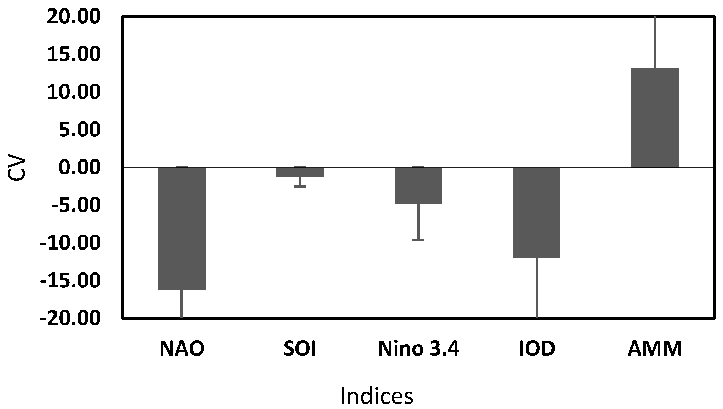
3.1. Coefficient of Variation

The coefficient of variation (CV), defined as the most common statistical tool, captures the dispersion in the data relative to the mean as the standard deviation divided by the mean [46] and measures the variability in a series of numbers independently of the measurement unit used for this process [47]. The monthly CV of the time series of the given indices has been adopted to evaluate and assess their variability. Figure 1 and

Table 2. Monthly Averages, Standard Deviation (SD) and coefficient of variation (CV) for climatic Indices. The value between brackets is the absolute value of average and CV.

Indices	Average	SD	CV
NAO	−0.07 (0.07)	1.08	−16.18 (16.18)
SOI	−1.21 (1.21)	1.52	−1.26 (1.62)
Nino 3.4	−0.18 (0.18)	0.85	−4.82 (4.82)
IOD	−0.03 (0.03)	0.34	−12.02 (12.02)
AMM	0.19	2.51	13.14

reveal a highly positive value for the AMM of 13.4 (it is the only index with a positive CV value). In contrast, the remaining indices indicate negative values ranging from −1.26 to −16.18 during the study period. A negative CV value is due to a negative value of the mean. It is advised to utilize the mean without sign module for improved CV comparison. As a result, the index CVs are positive. These results show a relatively high variability in the time series of all indices, especially the NAO, IOD, and AMM indices, because the CV is greater than 1. The degree of uniformity and the consistency in the distribution of the index datasets indicate that the NAO, IOD, and AMM climatic indices are less uniform and less consistent than the SOI and ENSO. The standard deviation of the monthly variation listed in Table 2 indicates slightly positive values (ranging from 0.32 to 2.51) for most of the climate indices with consistent relationships. Although there is no notable difference in the standard deviation, there are large differences in the CV due its high sensitivity to the average.

3.2. Trend Analysis of Global Climatic Indices

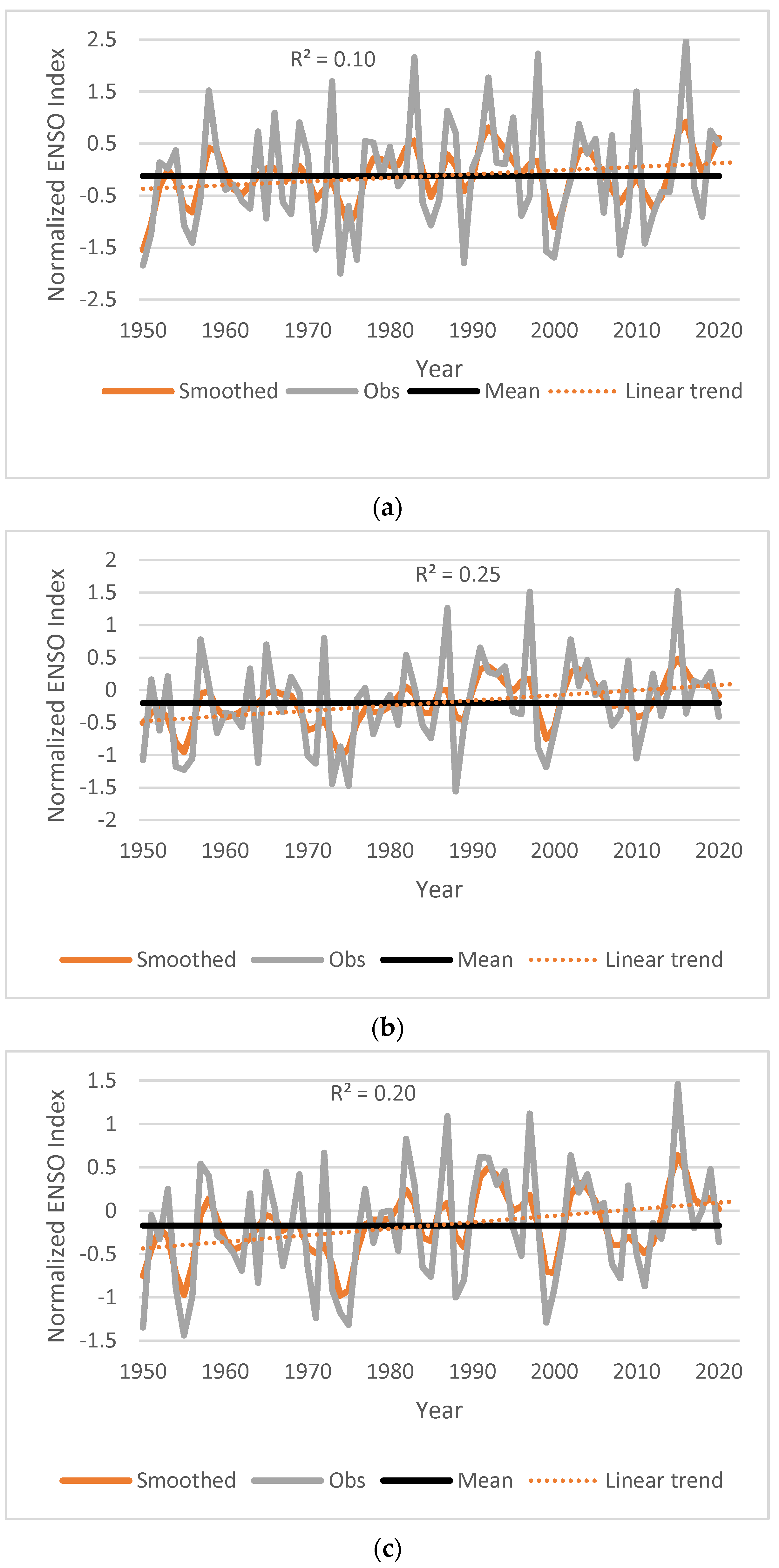
3.2.1. Trend Analysis of the ENSO Index

The trend analysis using the running mean filtering method in the ENSO index (Figure 2a–c) show that the smoothed and observational time series continue to exhibit a favorable match in the winter, summer, and annual results. In addition, this indicates an increasing trend in the ENSO index during the study period (1950–2020). The trends of the time series of the ENSO (Nino 3.4) in the annual, summer and winter data range from positive to negative trends. The linear trends increase on an annual basis and during the summer and winter seasons but not significantly, with R² values less than 0.25. In general, one can show from Figure 2a–c the increase in the ENSO index from mid-1970’s up to the end of study. Increase and decrease in the ENSO index from year to year is observed. El Niño imposes warming effects on the world’s climate, but La Niña imposes an immediate cooling effect, which is often most significant in the year after occurrence. Positive and negative responses that occur naturally through the climate system are among the processes responsible for SST fluctuations in the tropical Pacific [20]. Moreover, El Niño episodes became common in the tropical Pacific throughout the 1980s and 1990s. Furthermore, a significant increase at 95% confidence level in the linear trend is observed in the summer season of ENSO. However, there is no significant increase in the linear trend of ENSO for both winter and annual time series. There remains a lack of knowledge regarding the mechanisms underlying decadal ENSO changes [48].

3.2.2. Trend Analysis of the SOI

The SOI index indicates a general decreasing trend in the summer and annual time series (Figure 3b,c), while in contrast, no changes are detected in the winter long-range trend, as shown in Figure 3a. Additionally, the smoothed and observational time series fluctuations are acceptable with positive and negative values throughout the study period. The decreasing linear trends in the SOI index in the annual, summer and winter time series are not significant because $R^{\mathbf{2}}$ is less than 14%. From the definition of the SOI, the positive phase represents an above-normal air pressure in Tahiti and a below-normal air pressure in Darwin. Long durations of positive (negative) SOI values correspond with the unusually cold (warm) ocean waters that are characteristic of La Niña (El Niño) events in the eastern tropical Pacific. Additionally, the Walker circulation strength can be determined by the SOI, which is considered one of the most important atmospheric indicators for determining the intensity of El Niño and La Niña occurrences. Figure 3a–c clearly show a decrease in the SOI from the mid-1970s up to the start or mid-1980s (according to the season) and over the last decade (2010–2020). The Walker circulation seems to be weakening as a result of both a natural increase in the frequency of El Niño events and a natural decrease in the frequency of La Niña events [49,50,51], as well as to a certain extent due to global warming [23,51,52]. Power and Smith examined the possibility that global warming might have contributed to some of the observed decreases in the value of the SOI after 1976 [51]. An increase in the SOI occurs approximately during the period from the mid-1960s to mid-1970s and from the mid-1980s up to the first decade of the 21st century. Power and Kociuba demonstrated that, contrary to expectations, the SOI tends to rise rather than fall during the 21st century [53]. The MSLP tends to rise in Darwin and Tahiti during global warming, while Tahiti tends to exhibit greater increases than Darwin. Tahiti is located in a vast area in which the MSLP tends to increase as a result of global warming. The SOI is thus a highly uncertain indicator of long-term tropical changes related to global warming, despite functioning as a suitable measure of yearly variability in both the equatorial MSLP gradient and the WC. The findings of Power and Kociuba also suggest that internal, naturally occurring variability is the primary cause of the first 21st-century decline in the SOI.

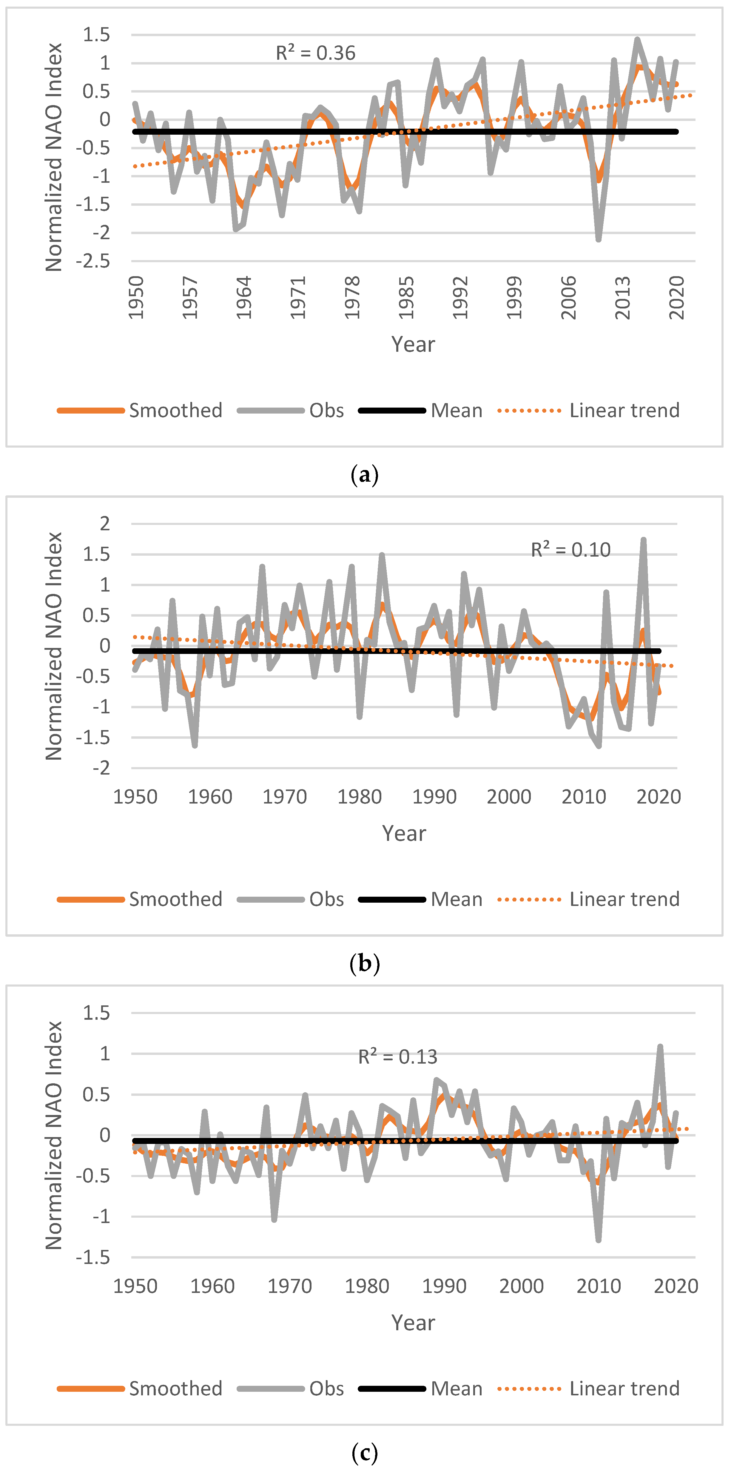
3.2.3. Trend Analysis of the NAO Index

Generally, the NAO index shows an increasing trend in the winter and annual time series (Figure 4a,c), while it exhibits a decreasing trend during the summer season (Figure 4b). Regarding the winter season NAO time series (Figure 4a), the 1950s up to mid-1960s showed decreasing trends and gradually increasing trends up to the start of the 1990s, then decreasing trends up to 2010 (mostly above the mean) and an increasing trend up to the end of the study period. The linear trend in the NAO winter series is a significant increasing trend, while the increasing trends of the NAO in the annual and summertime series are not significant. The winter NAO index tends to rise in most climate models as a result of rising greenhouse gas concentrations; however, these increases are often lower than those in reality, but overall, the mechanism of the response to greenhouse gases remains open to debate [54]. Regarding the summer NAO time series (Figure 4b), the 1950s showed decreasing trends and gradually increasing trends from the 1960s up to the mid-1990s, then decreasing trends up to 2010 and an increasing trend up to the end of the study period (still below the mean of the series). The NAO summer series showed a linear decreasing trend. Regarding the annual NAO time series (Figure 4c), the 1950s and 1960s showed decreasing trends, a gradually increasing trend up to the first 1990s, a decreasing trend to 2010 and then an increasing trend up to the end of the study period (2020). The linear trend in the series was a slightly increasing trend. A positive NAO index was associated with ozone increase over Greenland and/or its depletion over the Azores, as was the case at the start and end of the 20th century [55]. Ozone depletion at polar latitudes, particularly over Greenland and Iceland, could be attributed to the negative NAO phase, which was recorded in the middle of the last century [56].

3.2.4. Trend Analysis of the AMM Index

The smoothed AMM time series and the observational time series during the winter with the same sample size also exhibited favorable matching (Figure 5a), beginning with positive values (trends) from 1950 to 1970 and decreasing values during (negative trends) the mid-1970s and 1990s. The remainder of the time series was interspersed with positive trends in 2000 and 2010 and a declining trend at the end of the study period. During the summer season (Figure 5b), the change in AMM starts with positive trends over the first decade during the study period (1950 to 1960) and a declining trend during the 1970s followed by an increasing trend. During the rest of the period, the smoothed time series and the observational time series fluctuated between positive and negative trends in almost identical patterns with a top positive value at the beginning of each decade. The time series depicted in Figure 5c shows the annual variation of AMM with 11 smoothing algorithms. The figure clearly shows that the sample size of the smoothed time series is the same as that of the observational time series. Additionally, it shows that the fluctuation match between both records is satisfactory. The smoothed time series of the AMM starts with a positive value from 1950 to 1970, and thereafter, a significant decreasing trend occurs until approximately the mid-1970s. The remainder of the time series ranges from positive trends in 1980, 1998, 2004 and 2011 to negative trends in 1985 and 1993. Moreover, it gradually increased from the mid-1970s until the end of the period and did not return to its original value, which may be similar to an increase in the surface temperature under global warming. The trend in the wintertime series is approximately similar to the trend in the annual time series of the AMM. Therefore, the wintertime series of the AMM may impose a greater effect on the annual time series of the AMM than the summertime series of the AMM. There are no significant linear trends in the annual, summer and winter time series of the AMM, with an R² value of approximately zero.

The positive phase of the AMM is accompanied by considerable above-normal SST and southwest wind stress anomalies in the northern tropical Atlantic. This suggests that the baseline northeast trade winds are weakened over the northern tropical Atlantic, resulting in reduced wind-driven evaporation and consequently lower heat fluxes from the ocean into the atmosphere. In this situation, the ocean loses less heat, resulting in a higher SST. Regarding the negative phase of the AMM, opposite circumstances can be attained [57,58,59].

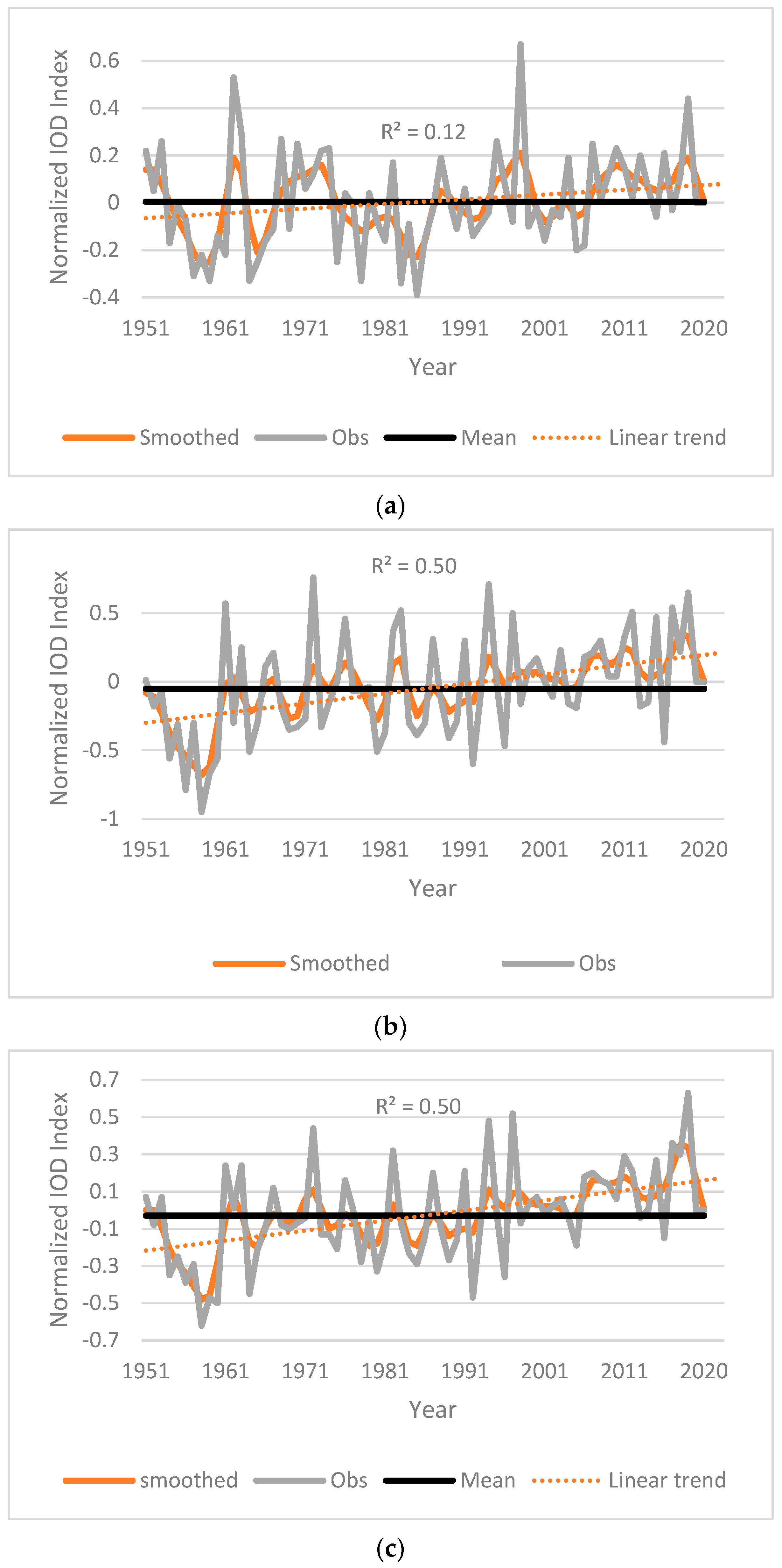
3.2.5. Trend Analysis of the IOD Index

A decreasing trend in the wintertime series of the IOD (Figure 6a) from the mid-1970s to mid-1990s is observed. An increasing trend in the wintertime series of the IOD index (Figure 6a) is found from the mid-1990s up to the end of the study period. The linear trends in the annual and summer IOD time series are significant positive trends (R² = 0.50), while the linear trend in the winter IOD time series is not significant (R² = 0.12).

Overall, the trend in the summertime series of the IOD index (Figure 6b) is similar to the trend of the annual time series of the IOD index (Figure 6c). The trend in the annual IOD index time series (Figure 6c) is a negative trend (decrease) over the first decade (1950s), a positive trend (increase) over the second decade (1960s), ranges from positive to negative trends or vice versa during the 1970s and 1980s, and then increases until the end of the study period. The linear trend in the annual IOD index time series is a significant increasing trend. There are a similarity of the trend analysis results for the annual, summer and winter time series of the IOD index, which starts from negative values at the beginning of the study period toward positive values at the end of the study period. Trend analysis of the winter, summer, and annual IOD index time series showed approximately the same trend, which decreased during the first decade of the 1950s.

Climate model projections of the response of the IOD to global warming are generally uncertain [60]. Additionally, strong positive IOD cool anomalies are caused by enhanced equatorial non-linear advection resulting from enhanced equatorial convection, which raises the temperature of the lower troposphere due to greenhouse warming. Consequently, the greenhouse effect is likely to increase the frequency of occurrence of climatic extremes compared to 2019 [61,62]. Evidence from other sources also points to a greater role of the tropical Indian Ocean in influencing the interannual climate variability [63].

Overall, the seasonal time series results indicate greater values (+ or −) than the annual values for most indices; interestingly, the trends in most cases start with negative values except the summer season for the SOI, NAO and AMM indices.

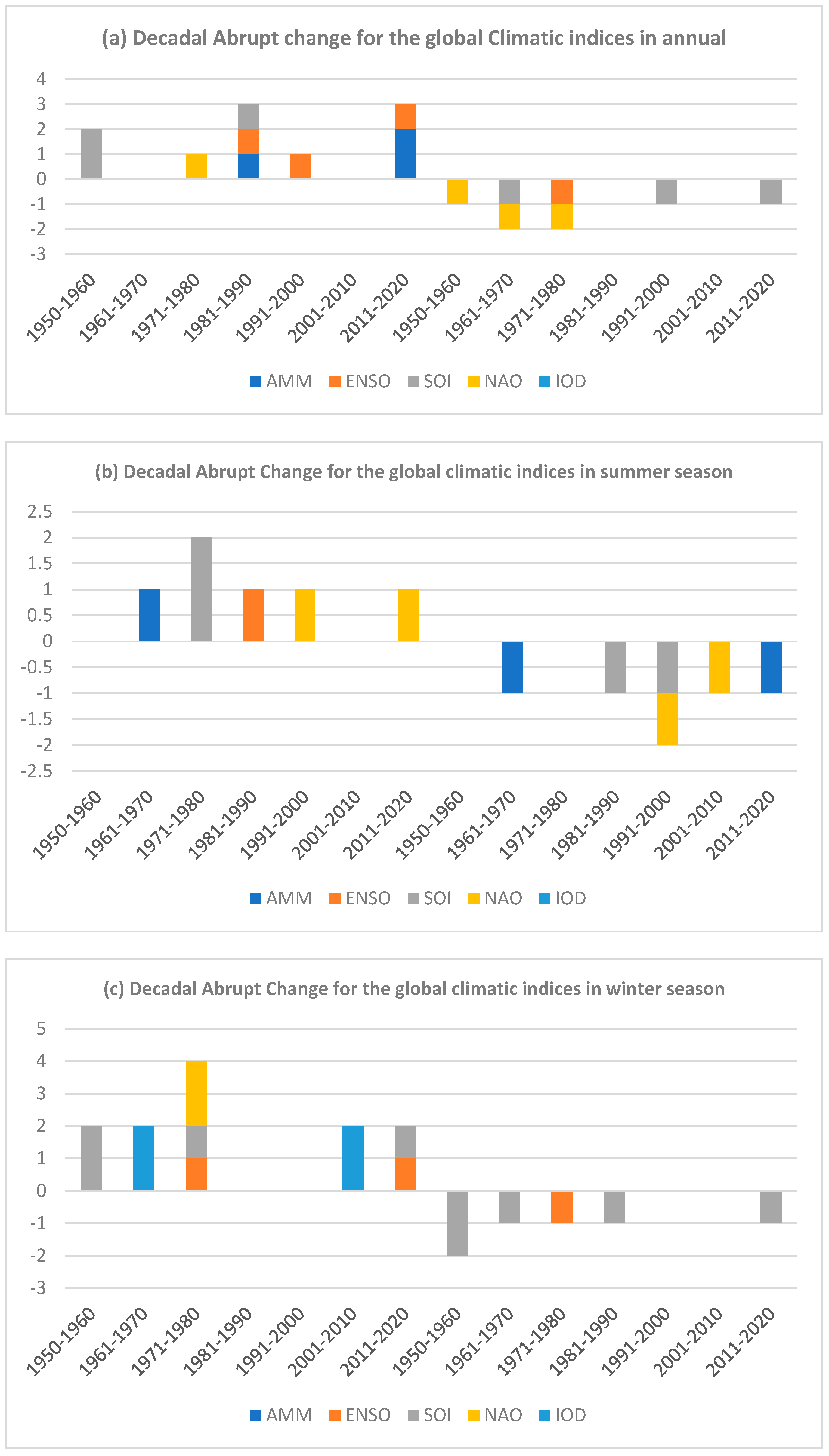
3.3. Abrupt Change in the Global Climatic Circulation Indices

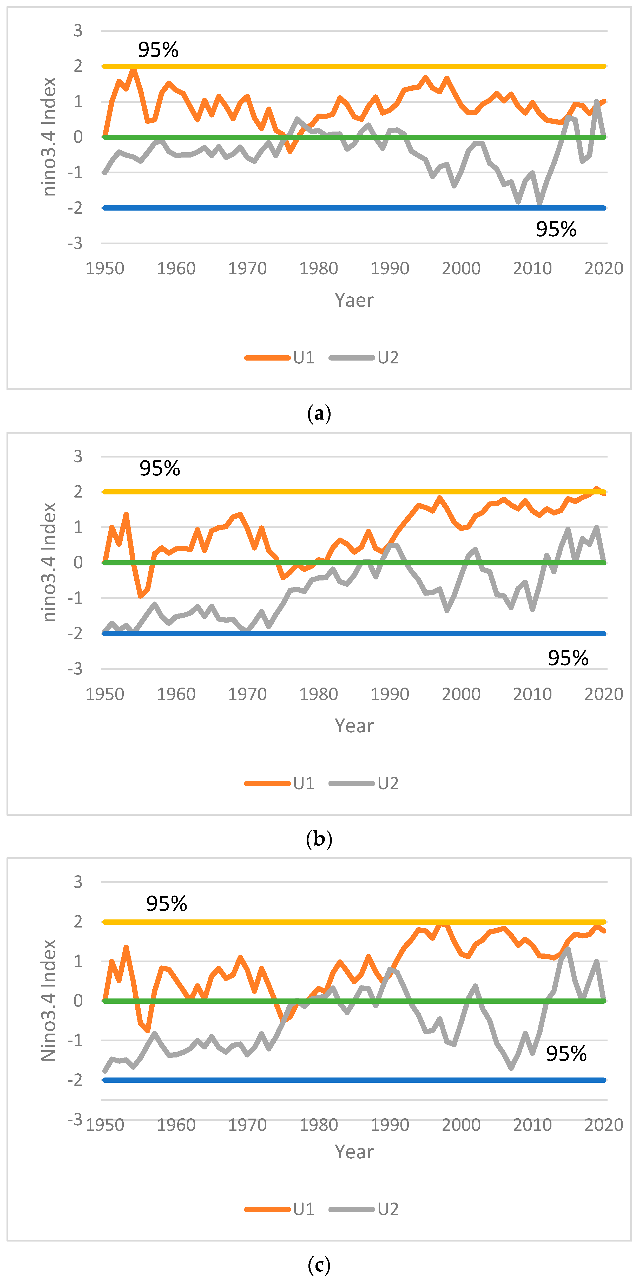
3.3.1. Abrupt Change in the ENSO Index

Figure 7a–c show the abrupt change in the ENSO index, which was obtained using the sequential form of the Mann-Kendall test for the winter, summer, and annual seasons (U1 forward sequential statistic and U2 backward sequential statistic, respectively). During the winter season (Figure 7a), there was an abrupt change (decreasing trend) in 1976 and an increasing trend in 1978 and 2019. In 2002 Rodo found a shift in the ENSO in 1976 that may possibly be linked to global warming [64]. Also, Rashid illustrated that forced changes in the ENSO are associated with global warming [65]. The abrupt change in the ENSO index during the summer season (Figure 7b) indicates an increasing trend in 1990 only. Figure 7c shows the Mann–Kendall t test results for the annual ENSO index. This figure illustrates annual positive abrupt changes in 1982, 1991, and 2015 and a negative abrupt change in approximately 1976. Similarly, other studies [66,67,68,69] have detected these changes, and they coupled and identified them with the ENSO cycle-related variability on an interannual timescale, which is also linked to climate change in general. Additionally, the time series are not smooth during the study period.

The observed trend toward positive values over the last 30 years of climate change in the tropical Pacific from approximately 1976 may be manifested both as shifting means and changing preferences in specific regimes [2]. Furthermore, there has been a rise in uncertainty in those climate change components that heavily depend on regional changes due to the importance of the ENSO and NAO as the primary drivers of regional climate change and their potential to trigger sudden shifts. The inference drawn from the observed ENSO variability is that small forcings could cause large changes in the behavior of this nonlinear system. The last two decades are marked by higher El Niño variability, including the two strongest El Niño events (1982/83 and 1997/98) over the 130 years of instrumental records and a prolonged warm spell in the early 1990s. This is in response to the apparent climate shift in the tropical Pacific in approximately 1976 [67,68], which is part of the recent tropical Pacific warming pattern [70,71]. Although attribution is dubious in light of the considerable natural variability observed [72] and the models’ inability to fully replicate the ENSO realistically, tropical Pacific warming may be linked to anthropogenic forcing [73].

There have been recorded multidecadal variations in the ENSO variability, although it is uncertain whether these shifts are caused by the ENSO cycle itself or by other types of climatic variability [74]. These records demonstrate the significant impact of the Atlantic on the ENSO multidecadal variability. The Walker circulation in the tropical Pacific Ocean is known to be forced by changes in Atlantic Multidecadal Oscillation-related tropical Atlantic SSTs. This demonstrates that these modifications to the Walker circulation affect the ENSO stability on both annual and multidecadal time scales, changing it in a way that produces a characteristic multidecadal ENSO variability pattern discovered in observations and ocean reanalysis.

3.3.2. Abrupt Change in the SOI

The winter season shows several abrupt changes, starting with positive trends in 1950, 1956, 1975 and 2013 and decreasing trends in 1952, 1958, 1964, 1986 and 2015 (Figure 8a). The summer season time series (Figure 8b) indicates that a positive increasing trend occurred in 1974 and 1979. There were decreasing abrupt changes in 1983 and 1991; thereafter, no changes occurred over the last decade of the study period. Figure 8c shows the significant positive abrupt change in the annual SOI in 1955, 1958, 1971, and 1987. In contrast, there were several decreasing trends (abrupt negative change) in 1965 and 1992 and more similar events starting in 2013. From the definition of the SOI, this index is one of the key atmospheric indices for gauging the strength of El Niño and La Niña events and their potential impacts, and from this perspective, the abrupt changes in the SOI might also be linked to the ENSO cycle-related variability on an interannual timescale, which also contributes to climate change in general.

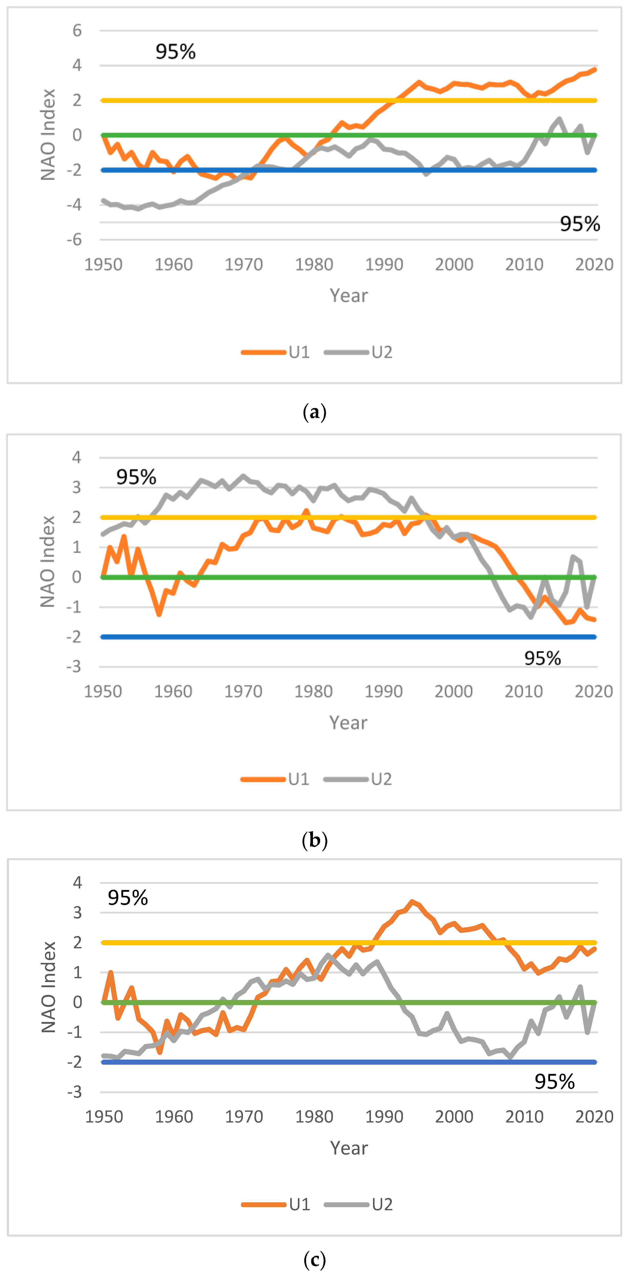
3.3.3. Abrupt Change in the NAO Index

The winter season time series (Figure 9a) shows only an increasing trend in a couple of years (1972 and 1979). Abrupt changes in the summer season time series start in the mid-1990s (1996), with a positive abrupt short-term change and another change in 2012 (Figure 9b). In contrast, negative abrupt changes occurred in 1999 and 2002. Figure 9c shows significant negative abrupt changes in 1958, 1963 and 1980 above the 95% confidence level. Additionally, a positive significant trend (increasing) starts in 1974 and in 1983, after which no abrupt change occurs until the end of the study period. The observed trend in the NAO index toward positive values over the past 30 years starting in 1976 [2] suggests that climate change may be seen as both shifting and changing in some regimes. Negative events occurred when the zonal flow across the Atlantic Ocean was weaker than usual, while positive episodes occurred when westerlies were stronger than usual [75]. The sudden NAO phase reversal is due to the change in the propagation direction of Rossby waves over northeastern North America due to the ENSO [76]. This change is mostly controlled by a climatological alteration in the local jet meridional shear. They also showed how the inherent eddy-low-frequency flow feedback in the North Atlantic supports and amplifies the NAO responses. Regarding intra-seasonal climate forecasting in the Euro-Atlantic region, the abrupt NAO phase reversal signal is strong enough during the ENSO winter.

3.3.4. Abrupt Change in the Atlantic Meridional Mode (AMM)

Figure 10a shows the winter season time series that exhibits an increasing trend (abrupt change) in 1977 and a decreasing trend in 2014 and 2019. Figure 10b shows the Mann–Kendall t test results for the AMM on a seasonal (summer) basis. There is an abrupt change (increasing trend) in 1961 and a decreasing trend in 1964 and 2018. Figure 10c shows the Mann–Kendall t test results for the abrupt changes in the AMM on an annual basis. This reveals that abrupt climatic changes occurred at different times during the study period from 1950–2020. An increasing trend abruptly occurred in 1981, 2013, and 2016. These change points in the AMM might be related to the phases of the ENSO cycle. It is proposed that the Pacific and Atlantic modes are similar and controlled by physics essential to the ITCZ [38]. In addition, the episodic changes in climate variabilities accompanied by changes in atmospheric circulation may be linked to changes in the Atlantic Meridional Overturning Circulation (AMOC) [77], which conforms with the AMM structure [78]. The AMOC is an important component of the Earth’s climate system, characterized by a northward flow of warm, salty water in the upper layers of the Atlantic and a southward flow of colder water in the deep Atlantic. Furthermore, changes in this circulation pattern profoundly impact the global climate system, and it is very likely that the strength of the AMOC will decrease over the course of the 21st century in response to increasing levels of greenhouse gases [79,80]. Generally, the annual, summer and winter U1 and U2 vectors share the same patterns except for no abrupt changes during the 1980s in summer.

3.3.5. Abrupt Change in the IOD Index

In the case of the IOD, the summer and annual time series show that there are no significant abrupt changes during the study period (Figure 11b,c), while during the winter (Figure 11a), a positive trend is clearly observed involving abrupt changes in the early and mid-60s. Moreover, other positive trend values of abrupt changes occurred in 2006 and 2010. There is evidence that the declining Walker circulation plays a role in the occurrence of these out-of-season IOD events, but more research is necessary. If true, this suggests increased IOD activity and, consequently, increased unseasonable IOD events in a warming world [81].

Figure 12 summarizes the annual and seasonal (summer and winter) abrupt changes in the global climatic indices. The data in these figures are magnified in terms of any climatic patterns between the chosen indices on a decadal basis, and we search for relationships with atmospheric large-scale circulations such as Hadley, Ferrel, Walker and Polar cells. These variations transition from positive to negative results throughout the study period (1950–2020); certain indices show no abrupt changes annually, such as the IOD index, while there is no abrupt change in the AMM index during the winter season only. In contrast, the SOI indicates the most abrupt changes, especially annually, over the study period, with the exception of the decade from 2000 to 2010 and winter (from 1950 to 1990), with approximately equal positive and negative occasions of abrupt changes. In addition, the IOD indicates only positive changes during the summer (once from 1950–1960) and winter seasons (twice from 1961–1970 and 2001–2010), while the NAO shows positive results between 1971 and 1980 in winter and transitions from positive to negative values over the last three decades during the summer season. Similar to the IOD, ENSO exhibits a single positive abrupt change during the summer season while indicating two mixed instances during the winter season (1971–1980 and 2011–2020).

As a result of the previous outputs, there is no clear fixed pattern except that with each positive or negative change, there is a similar future change in direction in the subsequent decades, but without a guarantee or expectation that this will occur at a specific time. However, further investigation and measurement are needed to increase the degree of confidence in these findings. The correlation between the indices and atmospheric large-scale circulations is one reason why this pattern should be monitored and reviewed. Notably, The Ferrel and Hadley circulations in the atmosphere are enhanced at times of high NAO index values, and the warm phase of the ENSO is characterized by a weakening in the Pacific Walker circulation, western Pacific Hadley circulation, and Atlantic Hadley circulation and a strengthening in the eastern Pacific Hadley circulation [82]. Moreover, the strengthening in the Hadley circulation in the North Atlantic area during the 1950s is indicated by the Atlantic Hadley’s rising pressure [83]. The ENSO Modoki, North Pacific Oscillation (NPO), and NAO all influence the interannual variability in the Western Pacific Hadley cell [84]. Furthermore, another study [85] suggested that the pre-monsoon AMM modifies the pressure systems and monsoonal Hadley circulation over India, hence affecting the monsoon circulation intensity.

3.4. Relationship between the Global Climatic Circulation Indices

The CC values between the global climatic indices during the winter season are listed in

Table 3. (a) Correlation Coefficient between climatic circulation indices in winter season. (b) Correlation Coefficient between climatic circulation indices in summer season. (c) Correlation Coefficient between climatic circulation indices in winter season.

(a)
CC	AMM	IOD	ENSO	SOI	NAO
NAO	−0.24 *	0.06	−0.02	0.00	1.0
SOI	0.34 **	0.11	−0.88 **	1.0
ENSO	−0.30 *	0.07	1.0
IOD	0.15	1.0
AMM	1.0
(b)
CC	AMM	IOD	ENSO	SOI	NAO
NAO	−0.24 *	0.11	−0.09	−0.02	1.0
SOI	0.24 *	−0.44 **	−0.81 **	1.0
ENSO	−0.16	0.42 **	1.0
IOD	−0.24 *	1.0
AMM	1.0
(c)
CC	AMM	IOD	ENSO	SOI	NAO
NAO	−0.59 **	0.15	0.25 *	−0.22	1.0
SOI	0.45 **	−0.32 **	−0.87 **	1.0
ENSO	−0.59 **	0.39 **	1.0
IOD	−0.31 **	1.0
AMM	1.0

**: means 99% significant level. *: means 95% significant level.

a. The highest negative CC value (r = −0.88, at the 99% confidence level) is found between the ENSO and SOI. The SOI and AMM also show a highly significant correlation (99%) (r = 0.34). Additionally, negative CC values were observed between the ENSO and AMM with r = −0.30 at the 95% confidence level. The CC during the summer season (Table 3b) exhibits several positive and negative values and significant relationships between the indices. Highly negative CC values (−0.81) between the ENSO and SOI at the 99% confidence level are observed. Additionally, a negative association (−0.44) between the SOI and IOD is found. However, a positive relationship (0.42) between the ENSO and IOD is observed. Moreover, the association between the SOI and AMM is 0.24 at the 95% confidence level.

Table 3c shows the annual CC between the six global climatic circulation indices (NAO, SOI, ENSO, IOD, and AMM). Generally, a positive correlation was observed between the NAO and ESO at the 95% significance level (0.25). Moreover, the CC value between the annual SOI and AMM is 0.45 at the 99% significance level. However, negative CC values between the annual SOI and each of the IOD and ENSO events (−0.32 and −0.87, respectively) at the 99% significance level are found. In addition, the ENSO exhibits positive and negative CC values with three global climatic circulations (AMM and IOD) at the 99% confidence level (r = −0.59 and 0.39, respectively). The IOD exhibits an annual (positive and negative) CC value of −0.31 at the 99% confidence level with the AMM index. Notably, the NAO index has a negative relationship (r = −0.24, at the 95% significance level) with the AMM index during the winter and summer seasons and a highly negative relationship (r = −0.59, at the 99% significance level) annually.

Due to the interaction between these global circulations and the effect on each other, the question is now which two of these indices are the most correlated when removing the effects of the other indices. To investigate the annual and seasonal PC values for the global climatic indices used in this study, we kept 4 of these indices constant each time to obtain PC results for the other two indices. Here, 1, 2, 3, 4 and 5 denote the global climatic circulation indices NAO, ENSO, AMM, IOD, and SOI, respectively.

In the winter, summer, and annual time series (

Table 4. (a) Winter Partial Correlation between seasonal global climatic indices. (b) Summer Partial Correlation between seasonal global climatic indices. (c) Annual Partial Correlation between global climatic indices.

(a)
PC	r12.345	r13.245	r14.235	r15.234
1950–2020	−0.08	−0.24 *	0.11	−0.03
PC	r23.145	r24.135	r25.134
1950–2020	−0.05	0.36 **	−0.88 **
PC	r34.125	r35.124
1950–2020	0.15	0.11
PC	r45.123
1950–2020	0.34 **
(b)
PC	r12.345	r13.245	r14.235	r15.234
1950–2020	−0.17	−0.24	0.10	−0.09
PC	r23.145	r24.135	r25.134
1950–2020	0.04	0.16	−0.76 **
PC	r34.125	r35.124
1950–2020	−0.14	0.14
PC	r45.123
1950–2020	−0.14
(c)
PC	r12.345	r13.245	r14.235	r15.234
1950–2020	−0.17	−0.57 **	0.00	−0.12
PC	r23.145	r24.135	r25.134
1950–2020	−0.44 **	−0.18	−0.84 **
PC	r34.125	r35.124
1950–2020	−0.08	−0.20
PC	r45.123
1950–2020	0.04

* means 95% significant confidence level, and ** 99% significant confidence level.

a, Table 4b, and Table 4c, respectively), the ENSO and SOI indices are negatively correlated (r = −0.88, r = −0.76, and r = −0.84, respectively) at the 99% significance level, with the other indices kept constant. The SOI is a climatological variable that captures the El Niño state in the Pacific [86]. Ocean–atmosphere interactions in the tropical Pacific and the surrounding atmosphere cause ENSO occurrence. Positive temperature anomalies in the eastern equatorial Pacific help decrease the generally wide sea surface temperature gradient range in the tropical Pacific. The trade winds weakened as a result, and the SOI becomes abnormally negative. The initial positive temperature anomaly is strengthened by these reduced trade winds because they stop cold water from upwelling in the eastern equatorial Pacific [87]. The temperature anomaly in the east consequently decreases and drastically changes after the generation of these negative anomalies. Oscillations may be caused by tropical air–sea instability and the delayed negative feedback of subsurface ocean dynamics [88]. The ENSO and SOI indices are almost fully anti-correlated, with low SOI values (weak trade winds) matching abnormally high SSTs and vice versa. The strong link between these two indices illustrates the positive feedback between the ocean and the atmosphere that causes ENSO oscillations [89].

With the NAO, AMM, and SOI maintained constant, a positive relationship between the ENSO and IOD (r = 0.36, at the 99% significance level) during the winter season is found (Table 4a). Ham et al. A weakening link has been observed between the ENSO and the IOD mode after the 2000s and 2010s relative to the preceding two decades (1980s and 1990s) [90]. Their results showed that the relationship between the IOD from September-November and the ENSO index from December-February was weaker during the 1999–2014 period (0.21) than during the preceding two decades (1979–1998) (0.64). Additionally, the differences in the spatial patterns of ENSO evolution during the boreal spring and summer are linked to the weakening in ENSO-IOD coupling in the 2000s and 2010s. The link between the IOD and ENSO, a significant mode of the interannual climate variability, has been the subject of intense debate since the IOD was discovered [91,92]. Most IOD episodes are considered associated with the ENSO; however, others are considered to result from the natural oscillations in the tropical Indian Ocean [93,94]. Through a change in the Walker circulation, the ENSO impacts the IOD. For instance, an experiment using an atmosphere–ocean coupled model showed that the ENSO might cause the formation of the IOD to be postponed until the boreal summer, while IOD events unrelated to the ENSO could occur as early as the boreal spring [95]. The periodicity, strength, and formation processes of the IOD are influenced by the ENSO variability in years of co-occurrence [96], although the IOD may also impact ENSO development [97]. A growing IOD is intensified and sustained when an El Niño event also occurs. The IOD can arise even in the absence of such an El Niño event or the related reinforcing air–sea interaction from the tropical Pacific, but it typically does so during the austral winter and ends within the season [81].

There exists no relationship between the ENSO and NAO based on partial correlation analysis, and only a weak positive relationship between these indices is found when using classical correlation (Table 4a). Only on an annual basis is the positive relationship between the NAO and ENSO in classical correlation analysis weak but statistically significant. A weak negative correlation between the two during the winter season, suggesting that a positive NAO phase may favor La Niña conditions [98,99]. However, the relationship is complex and can vary over time. The spatial correlation between the ENSO-related atmospheric pattern and the traditional NAO pattern is 0.86 and 0.85 in January and February, respectively [100]. The NAO causes a north-south dipole response over the North Atlantic throughout winter and spring, with potentially linked interactions with the ENSO stemming from the Pacific pool in winter [101]. The stability of linkages over time was examined using a running correlation for specific common global atmospheric and oceanic teleconnection indicators with a 35-year window width.

Keeping the ENSO, IOD, and SOI constant, the NAO is negatively associated with the AMM in winter and summer (r = −0.24, at the 95% confidence level)) and annually (r = −0.57, at the 99% confidence level). According to several studies [38,102,103,104,105], the NAO can stimulate the AMM through its southern portion of the Atlantic high. The North Atlantic Oscillation (NAO) exerts a significant impact on the development of the NTA and, consequently, the AMM [106,107,108]. However, further research is needed to determine how well models can simulate the NAO-AMM connection and its associated influence on the AMM. The AMO is likely a part of the mechanism that might force the AMM on decadal time scales [109]. The positive phase of AMO triggers wintertime negative phase of the NAO [110]. Both phenomena are related to variations in the strength and position of the Azores high-pressure system [98]. The lifetime of an AMM event begins in the boreal winter, when stochastic meteorological noise stemming from the Northern Hemisphere extratropics stretches into the subtropics and alters the strength of trade winds [111].

4. Conclusions

In this study, we examined the role of the variability in global climatic indices (ENSO, SOI, NAO, AMM, and IOD) and attempted to determine the relationship between these climatic indices during the period from 1950 to 2020. Monthly climatic index time series data were obtained from the NOAA PSL. Monthly average, standard deviation (SD) and coefficient of variation (CV) values of these climatic indices were calculated. Linear and nonlinear trend distributions of the time series on seasonal and annual bases were investigated. Moreover, abrupt changes throughout the study period in the annual and seasonal climatic indices were investigated, which indicate various significant positive to negative changes.

According to the CV results, all CV values of the climatic indices are negative due to a negative average value, with the exception of the CV value of the AMM. Moreover, all climatic index time series exhibit relatively high variability because the CV values are greater than 1.0. The NAO, IOD, and AMM climate indices are less uniform and less consistent than the SOI and ENSO, according to the degree of uniformity and consistency in the distribution of these index datasets.

Trend analysis of the annual time series for the AMM indicated a positive value from 1950 to 1970. Additionally, it steadily increased from the middle of the 1970s to the end of the period and did not return to its original value, which might be comparable to the increase in the surface temperature under global warming. During the summer season, the AMM exhibited a general decrease from 1950 up to the start of the 1970s, then increased up to 1980 and then fluctuated up to 2010, but it indicated a decrease over the last decade. The trend analysis results for the wintertime series are approximately similar to those for the annual time series. There are no obvious linear patterns in the annual, summer, or wintertime series of the AMM, and R² is close to zero. The annual, summer, and winter ENSO time series trends change from positive to negative. Winter and summer seasonal linear trends are rising but are not statistically significant, with an R² value less than 0.25. Over the study period, the SOI index annual, summer, and winter series values fluctuated between positive and negative values. The annual, summer, and winter declining linear trends in the SOI index were not notable. Generally, the annual NAO index showed a slowly increasing trend from the first period up to 1991 and then a decreasing trend up to 2010, while it indicated an increasing trend up to the end of 2020. The nonlinear trend in the summertime series illustrated a gradual increase from the first period up to the mid-1980s, and it decreased up to the end of the period. Regarding the winter season NAO time series, the period from the 1950s up to the mid-1960s showed decreasing trends and, in general, increasing trends up to the end of the study. While the rising trends in the NAO in the annual and summertime series were not considerable, the linear trend in the NAO winter series was a significant increasing tendency. The annual IOD index attained a downward trend in the 1950s, an upward trend in the 1960s, a fluctuating trend from positive to negative values or vice versa in the 1970s and 1980s, and then an upward trend to the end of the era. Generally, the summer IOD index pattern was similar to that of the annual IOD time series trend. Throughout the first decade of the 1950s and from the middle of the 1970s to the middle of the 1990s, the wintertime IOD index trend decreased. However, a rising trend in the wintertime series IOD index was observed from the middle of the 1990s until the end of the study period. The linear trend in the annual and summer IOD index time series was a significant increasing trend. The linear trend in the winter IOD time series was an increasing trend but not significant.

Regarding the abrupt change and considering the annual results, the SOI showed the largest number of abrupt change events ranging from positive to negative significant trends throughout the study period, while the IOD did not indicate any abrupt variations throughout the entire period. Another interesting finding is that the AMM showed positive trends only, especially over the last decade of the study period. In terms of seasonal changes, it exhibited more abrupt changes during the winter season than during the summer season, with approximately double the number of cases. Moreover, there were no changes in the AMM during the winter season. In contrast, the IOD indicated more increasing trends during the winter season than during the summer season (only one case).

Furthermore, we investigated the annual and seasonal (winter and summer) CC and PC values between the global climatic indices at the 95% and 99% confidence levels. In winter, the highest negative CC value was found between the ENSO and SOI. Additionally, statistically significant negative (positive) CC values occurred between the ENSO (SOI) and AMM. The CC values during the summer season indicated a highly negative (positive) relationship between the ENSO and SOI (IOD). Moreover, a highly negative association between the SOI and IOD was found, while a less positive association was found between the SOI and AMM. In the annual time series, there was a positive relationship between the ENSO and each of the NAO and IOD events, while there existed a negative relationship with each of the SOI and AMM events. Additionally, the SOI attained a positive (negative) association with the AMM (IOD). Moreover, the AMM index exhibited a negative association with the IOD index. In the winter and summer time series, it was evident that there exists a statistically negative association between the NAO index and the AMM index, while on an annual basis, a strongly negative relationship was discovered.

The ENSO and SOI indices, with the other indicators kept constant, were significantly negatively associated in the winter, summer, and annually time series, according to the PC results. A strong anti-correlation existed between the ENSO and SOI indices, with low SOI values (weak trade winds) corresponding to unusually high SSTs and vice versa. The close relationship between these two indices shows how the ocean and atmosphere positively interact to produce ENSO cycles [89]. The ENSO and IOD attained a very strong association during the winter season when the NAO, AMM, and SOI are absent. The ENSO affects the IOD by altering the Walker circulation. When an El Niño event also develops, a developing IOD is amplified and prolonged. When utilizing PC analysis, there is no association between the ENSO and NAO; nevertheless, when using classical correlation analysis, there exists only a weak positive relationship between these indices. However, the connection is complex and subject to change over time. Throughout winter and spring, the NAO is responsible for the north-south dipole reaction over the North Atlantic, with possible interactions with the ENSO from the Pacific pool in winter [101]. With the ENSO, IOD, and SOI kept unchanged, the NAO attains yearly and seasonal negative correlations with the AMM. When stochastic meteorological noise from the Northern Hemisphere extra tropics spreads into the subtropics and modifies the strength of trade winds, the boreal winter is when an AMM event first manifests itself [111].

References

1. Marengo, J.A.; Ambrizzi, T.; Barreto, N.; Cunha, A.P.; Ramos, A.M.; Skansi, M.; Molina Carpio, J.; Salinas, R. The heat wave of October 2020 in central South America. Int. J. Climatol. 2022, 42, 2281–2298. [Google Scholar] [CrossRef]
2. IPCC. Climate Change 2014. Impacts, Adaptation and Vulnerability. Working Group II Contribution to the IPCC Fifth Assessment Report; Cambridge University Press: Cambridge, UK, 2014. [Google Scholar]
3. Hurrell, J.W.; Deser, C. North Atlantic climate variability: The role of the North Atlantic Oscillation. J. Mar. Syst. 2010, 79, 231–244. [Google Scholar] [CrossRef]
4. Wang, G.; Schimel, D. Climate change, climate modes, and climate impacts. Annu. Rev. Environ. Resour. 2003, 28, 1–28. [Google Scholar] [CrossRef]
5. Walker, G.T. Probable amount of monsoon rainfall in 1920. Mon. Weather. Rev. 1920, 48, 415. [Google Scholar] [CrossRef]
6. Hurrell, J.W.; Kushnir, Y.; Ottersen, G.; Visbeck, M. An overview of the North Atlantic oscillation. Geophys. Monogr.-Am. Geophys. Union 2003, 134, 1–36. [Google Scholar]
7. Moraes, F.; Kooperman, G.; Mote, T. The combined and individual effects of the North Atlantic oscillation and the Atlantic meridional mode on early rainfall season precipitation in the insular Caribbean. In Proceedings of the AGU Fall Meeting 2019, San Francisco, CA, USA, 9–13 December 2019. [Google Scholar]
8. Veiga, S.M.F. The Influence of Oceanic and Atmospheric Large-Scale Variabilities on the Atlantic Meridional Mode Decadal the Scale. Ph.D. Thesis, Instituto Nacional de Pesquisas Espaciais—INPE Gabinete do Diretor (GBDIR), São José dos Campos, Brazil, 2018. Available online: http://urlib.net/8JMKD3MGP3W34R/3RATA2H (accessed on 2 April 2023).
9. Abram, N.J.; Hargreaves, J.A.; Wright, N.M.; Thirumalai, K.; Ummenhofer, C.C.; England, M.H. Palaeoclimate perspectives on the Indian Ocean dipole. Quat. Sci. Rev. 2020, 237, 106302. [Google Scholar] [CrossRef]
10. Pottapinjara, V.; Girishkumar, M.S.; Sivareddy, S.; Ravichandran, M.; Murtugudde, R. Reltion between the upper ocean heat content in the equatorial Atlantic during breal spring and the Indian monsoon rainfall during June-September. Int. J. Climatol. 2016, 36, 2469–2480. [Google Scholar] [CrossRef]
11. Park, J.Y.; Yeh, S.W.; Kug, J.S.; Yoon, J. Favorable connections between seasonal foot printing mechanism and El Niño. Clim. Dyn. 2013, 40, 1169–1181. [Google Scholar] [CrossRef]
12. Wu, L.; He, F.; Liu, Z.; Li, C. Atmospheric teleconnections of tropical Atlantic variability: Interhemispheric, tropical-extratropical, and cross-basin interactions. J. Clim. 2007, 20, 856–870. [Google Scholar] [CrossRef]
13. Thirumalai, K.; DiNezio, P.N.; Okumura, Y.; Deser, C. Extreme temperatures in Southeast Asia caused by El Niño and worsened by global warming. Nat. Commun. 2017, 8, 15531. [Google Scholar] [CrossRef]
14. Dai, A.; Wigley, T.M.L. Global patterns of ENSO-induced precipitation. Geophys. Res. Lett. 2000, 27, 1283–1286. [Google Scholar] [CrossRef]
15. Martens, B.; Waegeman, W.; Dorigo, W.A.; Verhoest, N.E.; Miralles, D.G. Terrestrial evaporation response to modes of climate variability. NPJ Clim. Atmos. Sci. 2018, 1, 43. [Google Scholar] [CrossRef]
16. Hardiman, S.C.; Dunstone, N.J.; Scaife, A.A.; Smith, D.M.; Knight, J.R.; Davies, P.; Claus, M.; Greatbatch, R.J. Predictability of European winter 2019/20: Indian Ocean dipole impacts on the NAO. Atmos. Sci. Lett. 2020, 21, e1005. [Google Scholar] [CrossRef]
17. Yoo, J.H.; Moon, S.; Ha, K.J.; Yun, K.S.; Lee, J.Y. Cases for the sole effect of the Indian Ocean Dipole in the rapid phase transition of the El Niño–Southern Oscillation. Theor. Appl. Climatol. 2020, 141, 999–1007. [Google Scholar] [CrossRef]
18. Alexander, M.; Scott, J. The influence of ENSO on air-sea interaction in the Atlantic. Geophys. Res. Lett. 2002, 29, 46-1–46-4. [Google Scholar] [CrossRef]
19. Li, B.; Li, Y.; Chen, Y.; Zhang, B.; Shi, X. Recent fall Eurasian cooling linked to North Pacific Sea surface temperatures and a strengthening Siberian high. Nat. Commun. 2020, 11, 5859. [Google Scholar] [CrossRef]
20. Timmermann, A.; An, S.-I.; Kug, J.-S.; Jin, F.-F.; Cai, W.; Capotondi, A.; Cobb, K.M.; Lengaigne, M.; McPhaden, M.J.; Stuecker, M.F.; et al. El Niño–southern oscillation complexity. Nature 2018, 559, 535–545. [Google Scholar] [CrossRef]
21. Chen, D.; Lian, T.; Fu, C.; Cane, M.A.; Tang, Y.; Murtugudde, R.; Song, X.; Wu, Q.; Zhou, L. Influence of westerly wind bursts on El Niño diversity. Nat. Geosci. 2015, 8, 339–345. [Google Scholar] [CrossRef]
22. McPhaden, M.J.; Santoso, A.; Cai, W. El Niño Southern Oscillation in a Changing Climate; Wiley: Hoboken, NJ, USA, 2020. [Google Scholar]
23. Collins, M.; An, S.-I.; Cai, W.; Ganachaud, A.; Guilyardi, E.; Jin, F.-F.; Jochum, M.; Lengaigne, M.; Power, S.; Timmermann, A.; et al. The impact of global warming on the tropical Pacific Ocean and El Niño. Nat. Geosci. 2010, 3, 391–397. [Google Scholar] [CrossRef]
24. Diaz, H.F.; Hoerling, M.P.; Eischeid, J.K. ENSO variability, teleconnections and climate change. Int. J. Climatol. A J. R. Meteorol. Soc. 2001, 21, 1845–1862. [Google Scholar] [CrossRef]
25. Latif, M.; Semenov, V.A.; Park, W. Super El Niños in response to global warming in a climate model. Clim. Change 2015, 132, 489–500. [Google Scholar] [CrossRef]
26. Bellenger, H.; Guilyardi, É.; Leloup, J.; Lengaigne, M.; Vialard, J. ENSO representation in climate models: From CMIP3 to CMIP5. Clim. Dyn. 2014, 42, 1999–2018. [Google Scholar] [CrossRef]
27. Namias, J. Basis for prediction of the sharp reversal of climate from autumn to winter 1988–1989. Int. J. Climatol. 1990, 10, 659–678. [Google Scholar] [CrossRef]
28. Overpeck, J.T.; Cole, J.E. Abrupt change in Earth’s climate system. Annu. Rev. Environ. Resour. 2006, 31, 1–31. [Google Scholar] [CrossRef]
29. Hansen, J.; Sato, M.; Glascoe, J.; Ruedy, R. A common-sense climate index: Is climate changing noticeably? Proc. Natl. Acad. Sci. USA 1998, 95, 4113–4120. [Google Scholar] [CrossRef] [PubMed]
30. Bjerknes, J. Atmospheric teleconnections from the equatorial pacific. Month. Weather Rev. 1969, 97, 163–172. [Google Scholar] [CrossRef]
31. Rasmusson, E.M.; Carpenter, T.H. Variations in tropical sea surface temperature and surface wind fields associated with the Southern Oscillation/El Niño. Monthly Weather Rev. 1982, 110, 354–384. [Google Scholar] [CrossRef]
32. Wallace, J.M.; Rasmusson, E.M.; Mitchell, T.P.; Kousky, V.E.; Sarachik, E.S.; von Storch, V. On the structure and evolution of climate variability in the tropical Pacific: Lessons from TOGA. J. Geophys. Res. 1998, 103, 14241–14259. [Google Scholar] [CrossRef]
33. Murray, D.; Hoell, A.; Hoerling, M.; Perlwitz, J.; Quan, X.-W.; Allured, D.; Zhang, T.; Eischeid, J.; Smith, C.A.; McWhirter, J.; et al. Facility for weather and climate assessments (FACTS): A community resource for assessing weather and climate variability. Bull. Am. Meteorol. Soc. 2020, 101, E1214–E1224. [Google Scholar] [CrossRef]
34. Climate Indices: Monthly Atmospheric and Ocean Time Series: National Oceanic and Atmospheric Administration (NOAA), Physical Sciences Laboratory (PSL). Available online: https://psl.noaa.gov/data/climateindices/list/ (accessed on 10 April 2023).
35. National Center for Atmospheric Research (NCAR). Available online: https://climatedataguide.ucar.edu/climate-data/nino-sst-indices-nino-12-3-34-4-oni-and-tni (accessed on 10 April 2023).
36. National Climate Centre (NCC), Bureau of Meteorology (BOM). Available online: http://www.bom.gov.au/climate/ahead/about-ENSO-outlooks.shtml (accessed on 10 April 2023).
37. Barnston, A.G.; Livezey, R.E. Classification, seasonality and persistence of low-frequency atmospheric circulation patterns. Mon. Weather. Rev. 1987, 115, 1083–1126. [Google Scholar] [CrossRef]
38. Chiang, J.C.H.; Vimont, D.J. Analogous Pacific and Atlantic Meridional Modes of Tropical Atmosphere–Ocean Variability. J. Clim. 2004, 17, 4143–4158. [Google Scholar] [CrossRef]
39. Carton, J.A.; Giese, B.S.; Grodsky, S.A. Sea level rise and the warming of the oceans in the Simple Ocean Data Assimilation (SODA) ocean reanalysis. J. Geophys. Res. Ocean. 2005, 110. [Google Scholar] [CrossRef]
40. Doi, T.; Tozuka, T.; Yamagata, T. The Atlantic meridional mode and its coupled variability with the Guinea Dome. J. Clim. 2010, 23, 455–475. [Google Scholar] [CrossRef]
41. Sneyers, R. On the statistical analysis of series of observations (No. 143). In Technical Note; World Meteorological Organization: Geneva, Switzerland, 1991; 218p. [Google Scholar]
42. Goossens, C.; Berger, A. Annual and seasonal climatic variations over the northern hemisphere and Europe during the last century. Ann. Geophys. 1986, 4, 385. [Google Scholar]
43. Hu, F.S.; Ito, E.; Brubaker, L.B.; Anderson, P.M. Ostracode geochemical record of Holocene climatic change and implications for vegetational response in the northwestern Alaska Range. Quat. Res. 1998, 49, 86–95. [Google Scholar] [CrossRef]
44. Shapiro, R. Linear filtering. Math. Comput. 1975, 29, 1094–1097. [Google Scholar] [CrossRef]
45. Nigam, S. In Teleconnection. In Encyclopedia of Atmospheric Science; Holton, J.R., Pyle, J., Curry, J.A., Eds.; Academic Press: Cambridge, MA, USA; Elsevier Science Ltd.: Amsterdam, The Netherlands, 2003; Volume 6, pp. 2243–2269. [Google Scholar]
46. Lovie, P. Coefficient of variation. Encycl. Stat. Behav. Sci. 2005, 1. [Google Scholar]
47. Abdi, H. Coefficient of variation. Encycl. Res. Des. 2010, 1, 1–5. [Google Scholar]
48. Zhang, R.-H.; Gao, C.; Feng, L. Recent ENSO evolution and its real-time prediction challenges. Natl. Sci. Rev. 2022, 9, nwac052. [Google Scholar] [CrossRef]
49. Trenberth, K.E.; Hoar, T.J. El Niño and climate change. Geophys. Res. Lett. 1997, 24, 3057–3060. [Google Scholar] [CrossRef]
50. Folland, C.K.; Karl, T.R.; Christy, J.R.; Clarke, R.A.; Gruza, G.V.; Jouzel, J.; Mann, M.E.; Oerlemans, J.; Salinger, M.J.; Wang, S.-W. Observed climate variabiltiy and change. In Climate Change 2001: The Scientific Basis. Contributions of WG1 to the Third Assessment Report of the IPCC; Houghton, J.T., Ed.; Cambridge University Press: Cambridge, UK, 2001; p. 881. [Google Scholar]
51. Power, S.B.; Smith, I.N. Weakening of the Walker circulation and apparent dominance of El-Nino both reach record levels, but has ENSO really changed? Geophys. Res. Lett. 2007, 34. [Google Scholar] [CrossRef]
52. Vecchi, G.A.; Soden, B.J.; Wittenberg, A.T.; Held, I.M.; Leetmaa, A.; Harrison, M.J. Weakening of the topical atmospheric circulation due to anthropogenic forcing. Nature 2006, 419, 73–76. [Google Scholar] [CrossRef]
53. Power, S.B.; Kociuba, G. The impact of global warming on the Southern Oscillation Index. Clim. Dyn. 2011, 37, 1745–1754. [Google Scholar] [CrossRef]
54. Gillett, N.P.; Graf, H.F.; Osborn, T.J. Climate change and the North Atlantic oscillation. Geophys. Monogr.-Am. Geophys. Union 2003, 134, 193–210. [Google Scholar]
55. Kilifarska, N.A.; Bakhmutov, V.G.; Melnyk, G.V. The Hidden Link between Earth’s Magnetic Field and Climate. In Chapter 8—Geomagnetic Field and Internal Climate Modes; Elsevier: Amsterdam, The Netherlands, 2020; ISBN 978-0-12-819346-4. [Google Scholar]
56. Velichkova, T.; Kilifarska, N. Lower stratospheric ozone’s influence on the NAO climatic mode. Comptes Rendus De L’acade’mie Bulg. Des Sci. 2019, 72, 219–225. [Google Scholar] [CrossRef]
57. Xia, F.; Zuo, J.; Sun, C.; Liu, A. The Atlantic Meridional Mode and Associated Wind–SST Relationship in the CMIP6 Models. Atmosphere 2023, 14, 359. [Google Scholar] [CrossRef]
58. Chang, T.-C.; Hsu, H.H.; Hong, C.-C. Enhanced influences of tropical Atlantic SST on WNP-NIO atmosphere-ocean coupling since the early 1980s. J. Clim. 2016, 29, 6509–6525. [Google Scholar] [CrossRef]
59. Hong, C.-C.; Chang, T.-C.; Hsu, H.-H. Enhanced relationship between the tropical Atlantic SST and the summertime western North Pacific subtropical high after the early 1980s. J. Geophys. Res. 2014, 119, 3715–3722. [Google Scholar] [CrossRef]
60. Hui, C.; Zheng, X.T. Uncertainty in Indian Ocean Dipole response to global warming: The role of internal variability. Clim. Dyn. 2018, 51, 3597–3611. [Google Scholar] [CrossRef]
61. Cai, W.; Yang, K.; Wu, L.; Huang, G.; Santoso, A.; Ng, B.; Wang, G.; Yamagata, T. Opposite response of strong and moderate positive Indian Ocean Dipole to global warming. Nat. Clim. Change 2021, 11, 27–32. [Google Scholar] [CrossRef]
62. Wang, G.; Cai, W. Two-year consecutive concurrences of positive Indian Ocean Dipole and Central Pacific El Niño preconditioned the 2019/2020 Australian “black summer” bushfires. Geosci. Lett. 2020, 7, 19. [Google Scholar] [CrossRef]
63. Zhang, L.; Han, W. Indian Ocean Dipole leads to Atlantic Niño. Nat. Commun. 2021, 12, 5952. [Google Scholar] [CrossRef]
64. Rodo, X.; Pascual, M.; Fuchs, G.; Faruque, A.S.G. ENSO and cholera: A nonstationary link related to climate change? Proc. Natl. Acad. Sci. USA 2002, 99, 12901–12906. [Google Scholar] [CrossRef] [PubMed]
65. Rashid, I.U.; Abid, M.A.; Almazroui, M.; Kucharski, F.; Hanif, M.; Ali, S.; Ismail, M. Early summer surface air temperature variability over Pakistan and the role of El Niño–Southern Oscillation teleconnections. Int. J. Climatol. 2022, 42, 5768–5784. [Google Scholar] [CrossRef]
66. Quinn, W.H.; Neal, V.T. Recent climate change and the 1982–1983 El Nino. In Proceedings of the 8th Annual Climate Diagnostic Workshop, Toronto, ON, Canada; NOAA: Washington, DC, USA, 1984; pp. 148–154. [Google Scholar]
67. Trenberth, K.E.; Hurrell, J.W. Decadal atmosphere-ocean variations in the Pacific. Clim. Dyn. 1994, 9, 303–319. [Google Scholar] [CrossRef]
68. Graham, N.E. Decadal-scale climate variability in the tropical and North Pacific during the 1970s and 1980s: Observations and model results. Clim. Dyn. 1994, 10, 135–162. [Google Scholar] [CrossRef]
69. Zhang, Y.; Wallace, J.M.; Iwasaka, N. Is climate variability over the North Pacific a linear response to ENSO? J. Clim. 1996, 9, 1468–1478. [Google Scholar] [CrossRef]
70. Ganachaud, A.; Wunsch, C. Improved estimates of global ocean circulation, heat transport and mixing from hydrographic data. Nature 2000, 408, 453–457. [Google Scholar] [CrossRef] [PubMed]
71. Trenberth, K.E.; Fasullo, J.T. An apparent hiatus in global warming? Earth’s Future 2013, 1, 19–32. [Google Scholar] [CrossRef]
72. Latif, M.; Kleeman, R.; Eckert, C. Greenhouse warming, decadal variability, or El Niño? An attempt to understand the anomalous 1990s. J. Clim. 1997, 10, 2221–2239. [Google Scholar] [CrossRef]
73. Knutson, T.R.; Manabe, S. Model assessment of decadal variability and trends in the tropical Pacific Ocean. J. Clim. 1998, 11, 2273–2296. [Google Scholar] [CrossRef]
74. Levine, A.F.Z.; McPhaden, M.J.; Frierson, D.M.W. The impact of the AMO on multidecadal ENSO variability. Geophys. Res. Lett. 2017, 44, 3877–3886. [Google Scholar] [CrossRef]
75. Jianping, L.; Wang, J.X.L. A new North Atlantic Oscillation index and its variability. Adv. Atmos. Sci. 2003, 20, 661–676. [Google Scholar] [CrossRef]
76. Kug, J.-S.; Geng, X.; Zhao, J. ENSO-driven abrupt phase shift in North Atlantic Oscillation in early January. Res. Sq. 2023. [Google Scholar] [CrossRef]
77. Kundzewicz, Z.W.; Pi’nskwar, I.; Koutsoyiannis, D. Variability of global mean annual temperature is significantly influenced by the rhythm of ocean-atmosphere oscillations. Sci. Total Environ. 2020, 747, 141256. [Google Scholar] [CrossRef] [PubMed]
78. Vimont, D.J. Analysis of the Atlantic meridional mode using linear inverse modeling: Seasonality and regional influences. J. Clim. 2012, 25, 1194–1212. [Google Scholar] [CrossRef]
79. Delworth, T.L.; Zeng, F. Simulated impact of altered Southern Hemisphere winds on the Atlantic meridional overturning circulation. Geophys. Res. Lett. 2008, 35. [Google Scholar] [CrossRef]
80. Lynch-Stieglitz, J. The Atlantic meridional overturning circulation and abrupt climate change. Annu. Rev. Mar. Sci. 2017, 9, 83–104. [Google Scholar] [CrossRef]
81. Du, Y.; Cai, W.; Wu, Y. A New Type of the Indian Ocean Dipole since the Mid-1970s. J. Clim. 2013, 26, 959–972. [Google Scholar] [CrossRef]
82. Wang, C. ENSO, Atlantic climate variability, and the walker and hadley circulations. In The Hadley Circulation: Present, Past and Future; Springer: Dordrecht, The Netherlands, 2004; pp. 173–202. [Google Scholar]
83. Iqbal, M.J.; Rehman, S.U.; Hameed, S.; Qureshi, M.A. Changes in Hadley circulation: The Azores high and winter precipitation over tropical northeast Africa. Theor. Appl. Climatol. 2019, 137, 2941–2948. [Google Scholar] [CrossRef]
84. Huang, R.; Chen, S.; Chen, W.; Yu, B.; Hu, P.; Ying, J.; Wu, Q. Northern poleward edge of regional Hadley cell over western Pacific during boreal winter: Year-to-year variability, influence factors and associated winter climate anomalies. Clim. Dyn. 2021, 56, 3643–3664. [Google Scholar] [CrossRef]
85. Vittal, H.; Villarini, G.; Zhang, W. Early prediction of the Indian summer monsoon rainfall by the Atlantic Meridional Mode. Clim. Dyn. 2020, 54, 2337–2346. [Google Scholar] [CrossRef]
86. Edgell, D.J. Correlation analysis of the El Nino-Southern Oscillation index and average temperatures and monthly precipitation totals in southeastern North Carolina. J. Elisha Mitchell Sci. Soc. 1999, 115, 71–81. [Google Scholar]
87. Stocker, T.F.; Clarke, G.K.C.; Le Treut, H.; Lindzen, R.S.; Meleshko, V.P.; Mugara, R.K.; Palmer, T.N.; Pierrehumbert, R.T.; Sellers, P.J.; Trenberth, K.E.; et al. Physical climate processes and feedbacks. In IPCC, 2001: Climate Change 2001: The Scientific Basis. Contribution of Working Group I to the Third Assessment Report of the Intergovernmental Panel on Climate Change; Houghton, J.T., Ding, Y., Griggs, D.J., Noguer, M., van der Linden, P.J., Dai, X., Maske, K., Eds.; Cambridge University Press: Cambridge, UK, 2001; pp. 417–470. [Google Scholar]
88. Neelin, J.D.; Battisti, D.S.; Hirst, A.C.; Jin, F.-F.; Wakata, Y.; Yamagata, T.; Zebiak, S.E. 1998:ENSO theory. J. Geophys. Res. 1998, 103, 14261–14290. [Google Scholar] [CrossRef]
89. Mcphaden, M.J. Evolution of the 2006–2007 El Nino: The role of intraseasonal to interannual time scale dynamics. Adv. Geosci. 2008, 14, 219–230. [Google Scholar] [CrossRef]
90. Ham, Y.G.; Choi, J.Y.; Kug, J.S. The weakening of the ENSO–Indian Ocean Dipole (IOD) coupling strength in recent decades. Clim. Dyn. 2017, 49, 249–261. [Google Scholar] [CrossRef]
91. Allan, R.; Chambers, D.; Drosdowsky, W.; Hendon, H.; Latif, M.; Nicholls, N.; Smith, I.; Stone, R.; Tourre, Y. Is There an Indian Ocean Dipole, and Is It Independent of the El Nino–Southern Oscillation? CLIVAR Exchanges, No. 6; International CLIVAR Project Office: Southampton, UK, 2001; pp. 18–22. [Google Scholar]
92. Yamagata, T.; Behera, S.K.; Rao, S.A.; Guan, Z.; Ashok, K.; Saji, H.N. The Indian Ocean Dipole: A Physical Entity. CLIVAR Exchanges, No. 24; International CLIVAR Project Office: Southampton, UK, 2002; pp. 15–22. [Google Scholar]
93. Yamagata, T.; Behera, S.K.; Luo, J.J.; Masson, S.; Jury, M.R.; Rao, S.A. Coupled ocean-atmosphere variability in the tropical Indian Ocean. Earth’s Climate: The Ocean-Atmosphere Interaction. Geophys. Monogr. Am. Geophys. Union 2004, 147, 189–211. [Google Scholar]
94. Meyers, G.; McIntosh, P.; Pigot, L.; Pook, M. The years of El Nino, La Nina, and interactions with the tropical Indian Ocean. J. Clim. 2007, 20, 2872–2880. [Google Scholar] [CrossRef]
95. Behera, S.K.; Luo, J.J.; Masson, S.; Rao, S.A.; Sakuma, H.; Yamagata, T. A CGCM study on the interaction between IOD and ENSO. J. Clim. 2006, 19, 1608–1705. [Google Scholar] [CrossRef]
96. Annamalai, H.; Xie, S.-P.; McCreary, J.P.; Murtugudde, R. Impact of Indian Ocean sea surface temperature on developing El Niño. J. Clim. 2005, 18, 302–319. [Google Scholar] [CrossRef]
97. Luo, J.J.; Behera, S.; Masumoto, Y.; Sakuma, H.; Yamagata, T. Successful prediction of the consecutive IOD in 2006 and 2007. Geophys. Res. Lett. 2008, 35, L14S02. [Google Scholar] [CrossRef]
98. Li, J.; Sun, C.; Jin, F.F. NAO implicated as a predictor of Northern Hemisphere mean temperature multi-decadal variability. Geophys. Res. Lett. 2013, 40, 5497–5502. [Google Scholar] [CrossRef]
99. Rodríguez-Fonseca, B.; Suárez-Moreno, R.; Ayarzagüena, B.; López-Parages, J.; Gómara, I.; Villamayor, J.; Mohino, E.; Losada, T.; Castaño-Tierno, A. A Review of ENSO Influence on the North Atlantic. A Non-Stationary Signal. Atmosphere 2016, 7, 87. [Google Scholar] [CrossRef]
100. Zhang, W.; Jiang, F. Subseasonal Variation in the Winter ENSO-NAO Relationship and the Modulation of Tropical North Atlantic SST Variability. Climate 2023, 11, 47. [Google Scholar] [CrossRef]
101. Patra, A.; Min, S.K.; Seong, M.G. Climate variability impacts on global extreme wave heights: Seasonal assessment using satellite data and ERA5 reanalysis. J. Geophys. Res. Ocean. 2020, 125, e2020JC016754. [Google Scholar] [CrossRef]
102. Xie, S.-P.; Tanimoto, Y. A pan-Atlantic decadal climate oscillation. Geophys. Res. Lett. 1998, 25, 2185–2188. [Google Scholar] [CrossRef]
103. Czaja, A.; Van der Vaart, P.; Marshall, J. A diagnostic study of the role of remote forcing in tropical Atlantic variability. J. Clim. 2002, 15, 3280–3290. [Google Scholar] [CrossRef]
104. Huang, B.; Shukla, J. Ocean–Atmosphere Interactions in the Tropical and Subtropical Atlantic Ocean. J. Clim. 2005, 18, 1652–1672. [Google Scholar] [CrossRef]
105. Penland, C.; Hartten, L.M. Stochastic forcing of north tropical Atlantic sea surface temperatures by the North Atlantic Oscillation. Geophys. Res. Lett. 2014, 41, 2126–2132. [Google Scholar] [CrossRef]
106. Chen, S.; Wu, R.; Chen, W. Strengthened connection between springtime North Atlantic Oscillation and North Atlantic tripole SST pattern since the late-1980s. J. Clim. 2020, 35, 2007–2022. [Google Scholar] [CrossRef]
107. Qiao, S.; Zou, M.; Tang, S.; Cheung, H.N.; Su, H.; Li, Q.; Feng, G.; Feng, G.; Dong, W. The Enhancement of the Impact of the Wintertime North Atlantic Oscillation on the Subsequent Sea Surface Temperature over the Tropical Atlantic since the Middle 1990s. J. Clim. 2020, 33, 9653–9672. [Google Scholar] [CrossRef]
108. Chen, S.; Wu, R.; Chen, W. The changing relationship between interannual variations of the North Atlantic Oscillation and northern tropical Atlantic SST. J. Clim. 2015, 28, 485–504. [Google Scholar] [CrossRef]
109. Veiga, S.F.; Giarolla, E.; Nobre, P.; Nobre, C.A. Analyzing the Influence of the North Atlantic Ocean Variability on the Atlantic Meridional Mode on Decadal Time Scales. Atmosphere 2019, 11, 3. [Google Scholar] [CrossRef]
110. Gastineau, G.; Frankignoul, C. Influence of the North Atlantic SST variability on the atmospheric circulation during the twentieth century. J. Clim. 2015, 28, 1396–1416. [Google Scholar] [CrossRef]
111. Amaya, D.J. The Pacific meridional mode and ENSO: A review. Curr. Clim. Change Rep. 2019, 5, 296–307. [Google Scholar] [CrossRef]
Figure 1. Monthly Coefficient of Variation for Indices.
Atmosphere 14 01741 g001
Figure 2. Trend analysis for ENSO index (a) Winter season, (b) Summer season, and (c) Annual.
Atmosphere 14 01741 g002
Figure 3. Trend analysis for Southern Oscillation Index (SOI) (a) Winter season, (b) Summer season, and (c) Annual.
Atmosphere 14 01741 g003
Figure 4. Trend analysis for North Atlantic Oscillation Index (NAO) (a) Winter season, (b) Summer season, and (c) Annual.
Atmosphere 14 01741 g004
Figure 5. Trend analysis for Atlantic Meridional Mode (AMM) (a) Winter season, (b) Summer season, and (c) Annual.
Atmosphere 14 01741 g005
Figure 6. Trend analysis for Indian Ocean Dipole (IOD) (a) Winter season, (b) Summer season, and (c) Annual.
Atmosphere 14 01741 g006
Figure 7. Abrupt change for ENSO index as derived from sequential version of the Mann-Kendall test (a) Winter season, (b) Summer season, and (c) Annual (U1 forward sequential statistic and U2 backward sequential statistic).
Atmosphere 14 01741 g007
Figure 8. Abrupt change for the Southern Oscillation Index (SOI) as derived from sequential version of the Mann-Kendall test. (a) Winter season, (b) Summer season, and (c) Annual (U1 forward sequential statistic and U2 backward sequential statistic).
Atmosphere 14 01741 g008
Figure 9. Abrupt change for the North Atlantic Oscillation (NAO) as derived from sequential version of the Mann-Kendall test. (a) Winter season, (b) Summer season, and (c) Annual (U1 forward sequential statistic and U2 backward sequential statistic).
Atmosphere 14 01741 g009
Figure 10. Abrupt change for Atlantic Meridional Mode (AMM) index as derived from sequential version of the Mann-Kendall test. (a) Winter season, (b) Summer season, and (c) Annual (U1 forward sequential statistic and U2 backward sequential statistic).
Atmosphere 14 01741 g010
Figure 11. Abrupt change for the Indian Ocean dipole (IOD) as derived from sequential version of the Mann-Kendall test (a) Winter season, (b) Summer season, and (c) Annual (U1 forward sequential statistic and U2 backward sequential statistic).
Atmosphere 14 01741 g011
Figure 12. Decadal abrupt change for the global climatic indices (a) annual, (b) Summer season, and (c) winter season.
Atmosphere 14 01741 g012