Article

Roles of Air–Sea Interactions in the Predictability of Typhoon Mawar and Remote Heavy-Rainfall Events after Five Days

Meteorological Research Institute, Japan Meteorological Agency, 1-1 Nagamine, Tsukuba 305-0052, Ibaraki, Japan
Atmosphere 2023, 14(11), 1638; https://doi.org/10.3390/atmos14111638
Submission received: 2 October 2023 / Revised: 25 October 2023 / Accepted: 30 October 2023 / Published: 31 October 2023
(This article belongs to the Special Issue Weather and Climate Extremes: Observations, Modeling, and Impacts)

Abstract

:
This study investigated the relationship between the predicted track of Typhoon Mawar (2023) and the quasi-stationary front along the southern coast of Japan where heavy rainfall occurred. Also, the role of ocean coupling was explored by using global model predictions and numerical simulations conducted by a regional atmosphere–wave–ocean coupled model. The track predictions by four major global models showed that the prediction errors became significantly larger after the recurvature. One of the global models could reasonably predict both the track and the location of the front, even after five days. The results of numerical simulations of which the initial and boundary conditions were based on the successful predictions suggest that ocean coupling contributes to the improvement of central pressure simulations compared with fixed oceanic conditions. More northward translation of Mawar after the recurvature simulated by the coupled model could be explained by the separation of the inner-core vortex into two parts in the upper and lower troposphere. However, the predictability of the Subtropical High was more important in determining not only the track but also environmental southerly flow over the moisture road formed between Mawar and the Subtropical High and in accurately predicting the location of the front.

1. Introduction

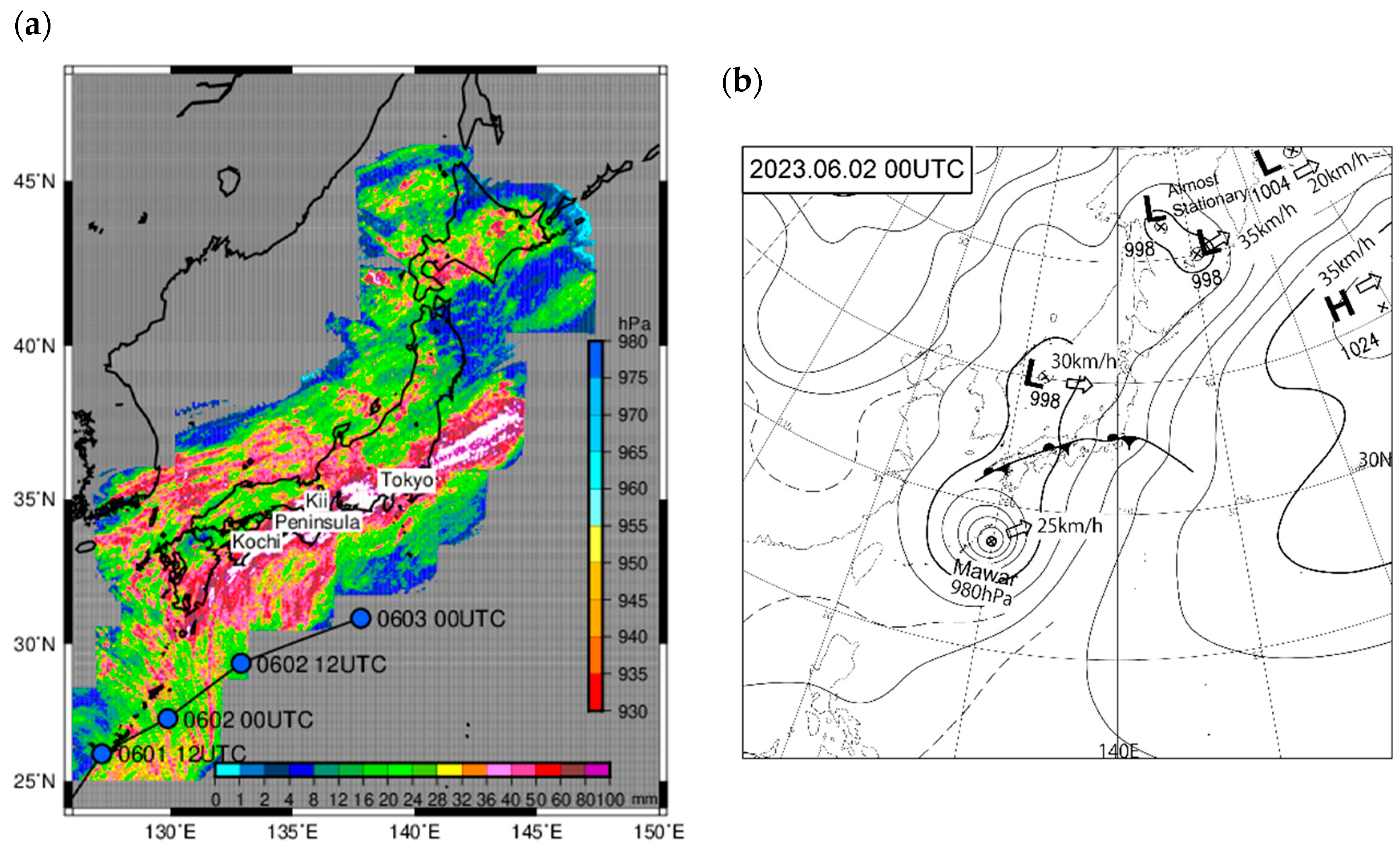
1.1. Typhoon Mawar and the Quasi-Stationary Front

In the western North Pacific, the average tropical cyclone (TC) occurrence has been approximately 26 since 1951 when the statistics started, with just under three making landfall in Japan. When a TC approaches Japan, it causes serious disasters due to high winds, torrential rains, storm surges, and high ocean waves. Therefore, the forecasting of TCs and associated extreme weather events is of great social interest. In particular, Typhoon Mawar (2023) had a major impact on Japanese society, including the planned suspension of rail and air services.
Mawar was developed from a tropical depression southeast of Guam at 06 UTC on 20 May in 2023. It moved northward, slowing down and then becoming almost stationary near the island of Guam and then moved west–northwestward. Mawar experienced rapid intensification twice during its lifetime, and its peak central pressure reached 905 hPa according to the Regional Specialized Meteorological Center (RSMC) Tokyo preliminary analysis. After slowing down in the east of the Philippines, Mawar changed the track to the northeast (recurvature) and became an extratropical cyclone at 06 UTC on 3 June. The typhoon brought heavy rainfall and associated disasters mainly along the southern coast of Japan from 1 to 2 June. Figure 1a shows the horizontal distribution of the accumulated radar–rain gauge analyzed rainfall, and Figure 1b shows the weather map at 00 UTC on 2 June in 2023. The accumulated rainfall with a horizontal resolution of 5 km was calculated by summing the total rainfall amount within ten minutes based on radar observations calibrated with rain gauge measurements from the Japan Meteorological Agency (JMA) automated meteorological data acquisition system [1]. Heavy rainfall was analyzed over a wide area of Japan. In particular, a belt of areas over the stationary front along the southern coast of Japan recorded accumulated precipitation exceeding 100 mm for two days. Moreover, in the southern coastal areas of Japan, localized stagnant heavy rainfall areas were observed in places over a wide area, causing disasters and significant impacts on society in Japan. Such heavy rainfall events frequently occur over the quasi-stationary front in East Asia, particularly in China and Japan during the early summer rainy season, which is called Meiyu in Chinese and Baiu in Japanese [2]. The quasi-stationary front is usually called the ‘Meiyu–Baiu front’, but it is simply called a ‘front’ in this study.
In Figure 1a, Mawar moved northeastward over the southern oceans of mainland Japan without landfalling. Such remote heavy-rainfall events that are far from a typhoon sometimes occur in Japan [2,3,4]. A statistical analysis showed that remote precipitation tends to occur when TCs are located over the southern or southwestern oceans of mainland Japan and when the tracks of TCs are northward or changing to the northeast [3]. Predecessor rain events are well-known remote effects that are enhanced by a broad region of deep tropical moisture that is transported poleward to the front over mainland Japan [5]. A broad and deep area of moisture transport from the tropical ocean on a length scale of approximately 1000 km is called a ‘moisture road’, whereas an area on a length scale exceeding 2000 km is called an ‘atmospheric river’ in general [4]. Moisture conveyer belt [6] is another terminology that is associated with atmospheric rivers mainly induced by extratropical cyclones. The elongated band of enhanced poleward water vapor fluxes oriented from the Tropics is formed by a trough or a low cutoff at very low latitudes [7]. The poleward transport of moisture is enhanced by an increase in the pressure gradient between a TC and a Subtropical High in addition to the moisture transport along the edge of the Subtropical High [2]. A change in the TC track affects the amount of poleward transport to the front by changing the location of the moisture road which, in turn, affects the amount of rainfall produced by the remote effect [2].

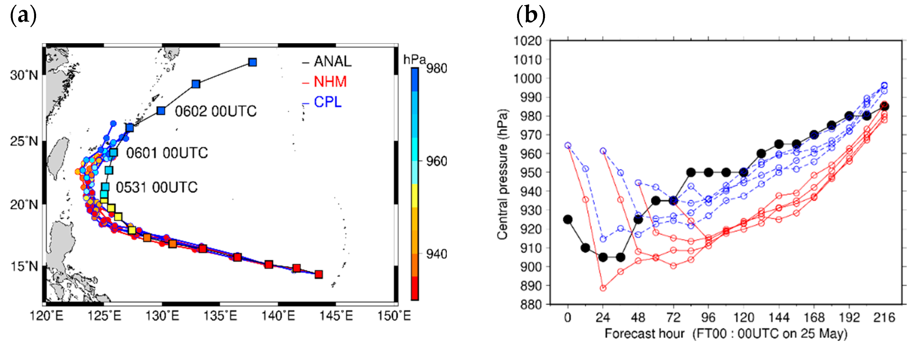
1.2. Predictability of Typhoon Mawar

If the heavy rainfall over the Meiyu–Baiu front along the southern coast of Japan (Figure 1a) is influenced by Mawar’s track, the longer the lead time for accurate track predictions, the better prepared we are for the onset of heavy rainfall in advance. Figure 2 shows the results of various Mawar’s track predictions at which the initial time was 00 UTC from 25 to 28 May in 2023. The data set was obtained from The Observing System Research and Predictability Experiment (THORPEX) Interactive Grand Global Ensemble (TIGGE) TC track model analysis and forecast data [8]. Deterministic TC track prediction data from the European Center for Medium-Range Weather Forecasts (ECMWF), the Japan Meteorological Agency (JMA), the National Centers for Environmental Prediction (NCEP), and the United Kingdom Met Office (UKMet) were used. The specifications of the global forecast model in each institute are shown in Table 1.
When comparing the results of TC track prediction among the above four major institutes, the uncertainty was greater during and after the recurvature of Mawar rather than before the recurvature (Figure 2a). The errors in track prediction were particularly large when the initial date was 25 May. Factors contributing to the track errors included both the continued northwestward movement without recurvature and the uncertain track direction after the recurvature. When compared with the RSMC Tokyo preliminary analysis, the relatively slow-moving speed predicted for Mawar also contributed to the increase in track errors.
Some model results predicted an excessive deepening of the central pressure around the recurvature area while moving excessively northwestward (Figure 2b). The excessive deepening around the recurvature area stood out in the JMA’s predictions, although the track prediction after the recurvature was the most reasonable among the four institutes (Figure 3). In other words, the other three institutes reasonably predicted the evolution of Mawar’s central pressure, although the track prediction was relatively poor compared to the JMA’s prediction. The effect of ocean coupling is considered to be one of the factors associated with the reasonable prediction of Mawar’s central pressure, since the ECMWF and UKMet global atmosphere–ocean coupled models could reasonably predict the central pressure.

1.3. Research Purposes
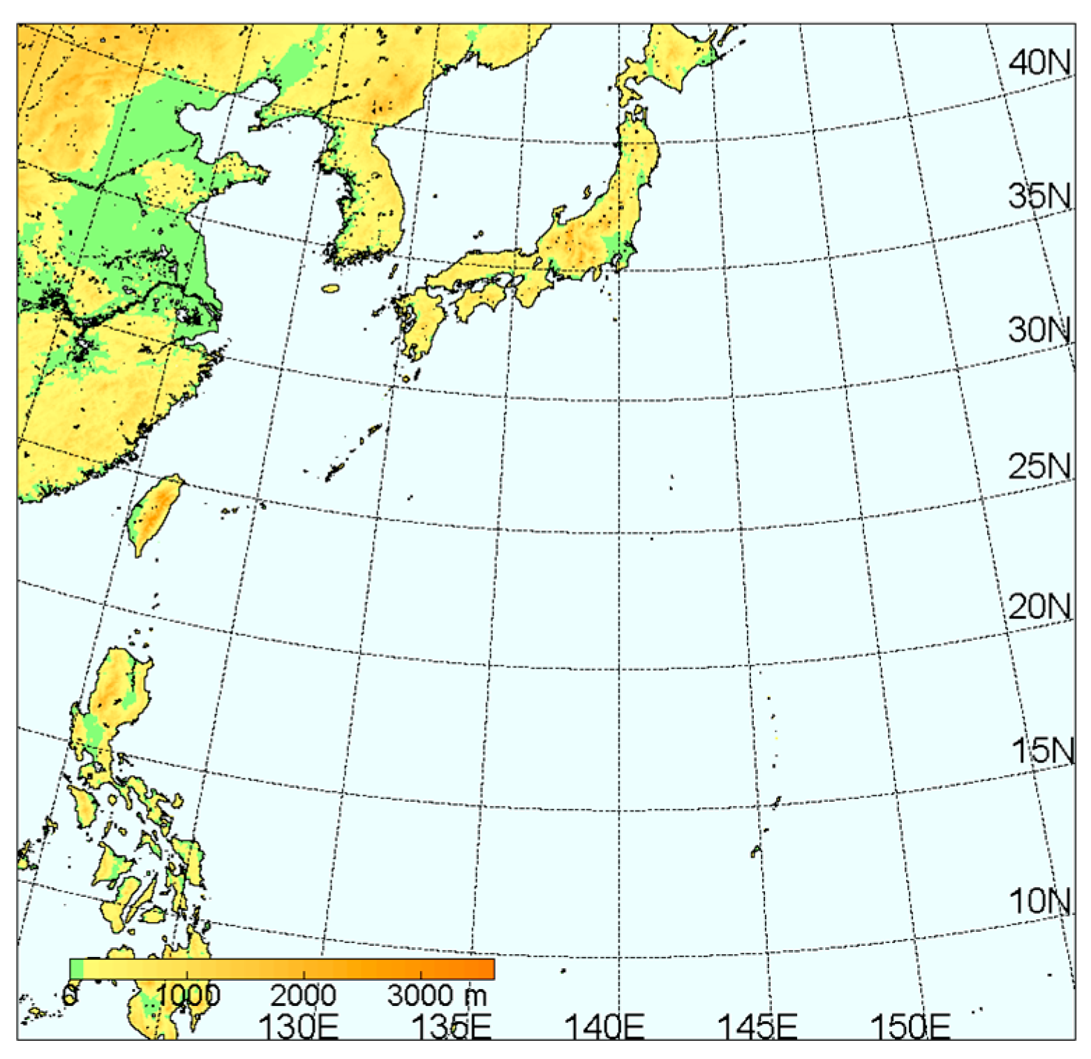
Numerical weather forecasting systems, as shown in Table 1, are constructed based on observation data, a data assimilation system, and a numerical model and are continuously being developed. Particularly in cases of extreme weather events, for which the prediction error is large, an in-depth investigation on the mechanism by using the model products will contribute to the idea that is necessary for making the prediction system more sophisticated. The extreme weather event associated with Mawar as well as the predictability of Mawar are appropriate cases to explore.
Therefore, the first purpose of this study is to show the predictability of the quasi-stationary front along the southern coast of Japan on 1–2 June when heavy rainfall was observed if the track prediction of Mawar followed the RSMC Tokyo preliminary analysis. The concern is whether or not the remote effect plays a crucial role in the rainfall event over the front. The second purpose is to assess the impact of ocean coupling on Mawar’s prediction when the track prediction by the global atmosphere model is reasonable but the prediction of the central pressure is excessive. The third purpose is to clarify the mechanism of Mawar’s predicted/simulated track after the recurvature and the associated heavy rainfall over the front along the southern coast of Japan, including a remote effect induced by Mawar in a framework of air–sea interactions.
The remainder of this paper is organized as follows: Section 2 briefly describes the global model data products, numerical models, their configuration, and the specifications for Mawar’s numerical simulations. Section 3 shows the results of the analyses with the JMA and NCEP global model data products and the numerical simulations performed by an atmosphere model and the regional atmosphere–wave–ocean coupled model. Section 4 discusses the effect of ocean coupling on the simulation of Mawar, the moisture road, and heavy rainfall over the front along the southern coast of Japan. Section 5 summarizes this study.

2. Data and Methods

First, NCEP and JMA global longitude–latitude grid products at which the initial time was 00 UTC on 25 and 28 May in 2023 were used to verify the synoptic-field prediction as well as Mawar’s track and rainfall predictions over the front along the southern coast of Japan on 1–2 June when heavy rainfall was observed. In addition, the JMA global longitude–latitude grid products at which the initial time was 00 UTC on 25–28 May in 2023 were used to create initial and lateral boundary conditions for numerical simulations by a regional nonhydrostatic atmosphere model (NHM) and the atmosphere–wave–ocean coupled model (CPL). The atmospheric physics used in the numerical simulations are shown in Table 2. The NHM included an explicit three-ice bulk microphysics scheme [9,10]. Air–sea momentum fluxes and sensible and latent heat fluxes, with exchange coefficients for air–sea momentum and enthalpy transfers over the sea, were based either on the bulk formulas of Kondo [11] for the NHM or on the roughness lengths proposed by Taylor and Yelland [12] in addition to a sea spray formulation [13] for the CPL. A turbulent closure model by Klemp and Wilhelmson [14] and Deardorff [15] and a radiation scheme by Sugi [16] were used for both the NHM and the CPL. No cumulus parameterization was used in the simulations.
The CPL consists of NHM [17], a Meteorological Research Institute (MRI) third-generation ocean surface-wave model [18], and an MRI multilayer ocean model based on the hurricane–ocean coupled model [19]. The MRI multilayer ocean model includes a diurnally varying SST scheme based on Schiller and Godfrey [20] with the shortwave absorption and penetration formulation of Ohlmann and Siegel [21]. The CPL has not been updated since the numerical simulation of Typhoon Haiyan in 2013 [13].
The model configuration is shown in Table 3. The integration was performed from 00 UTC on 25–28 May to 00 UTC on 4 June. The horizontal resolution of the NHM and CPL was 3 km in this study. The computational domain was single and covered the domain of 4500 km × 4320 km, centered at 25° N, 137° E in the Lamber Conformal Conic projection (Figure 4). The computational domain included synoptic features such as the Subtropical High, an area of heavy rainfall over the front along the southern coast of Japan (Figure 1) and a moisture road (or atmospheric river). The NHM used 55 levels in vertical coordinates, with intervals ranging from 40 m for the near-surface layer to 1013 m for the uppermost layer, and the top height was approximately 27 km.
The sea surface temperature (SST) at the initial time was derived from the Microwave Optimally Interpolated SST daily product with a horizontal resolution of 0.25° [22]. In order to create the oceanic initial conditions, this study used the North Pacific version of the Four-dimensional variational Ocean ReAnalysis data set for the western North Pacific (FORA) spanning 1996–2015 [23] and the subsequent oceanic analysis data that were operationally analyzed by the Japan Meteorological Agency from January 2016 (e.g., [24]). The horizontal resolution was 0.5° in the longitude–latitude coordinate system. The atmospheric initial and boundary conditions were created from the JMA six-hourly global model product with a horizontal grid spacing of approximately 10 km, although the horizontal resolution of the JMA global model was approximately 13 km (Table 1). The interval of the atmospheric boundary condition was 6 h (6 h).

3. Results

3.1. Results of Global Model Predictions

The products of the JMA and NCEP global models at which the initial time was 00 UTC on 25 and 28 May were used to verify the predictability of heavy rainfall over the front along the southern coast of Japan on 1–2 June (Figure 1). The JMA track prediction for Mawar at which the initial time was 00 UTC on 28 May was the most realistic prediction among the four predictions, in that it successfully predicted the northeastward movement after the recurvature (Figure 2). The JMA track prediction at which the initial time was 00 UTC on 25 May showed relatively slow northeastward motion. As for the NCEP products, the NCEP track prediction at which the initial time was 00 UTC on 25 May showed that the predicted Mawar tended to move eastward compared with the RSMC Tokyo preliminary analysis and the JMA global model predictions. The NCEP track predicton showed relatively slow translation before arriving at the recurvature area compared with the JMA prediction at the same initial time. In addition, the latitude of Mawar’s location predicted by the NCEP global model was relatively low compared with that of the JMA track predictions.
Figure 5 shows the horizontal distributions of the predicted precipitation amount summed every 6 h from 00 UTC on 1 June to 00 UTC on 3 June in 2023. Although the temporal resolution of the JMA and NCEP global-model products was relatively coarse compared to the analysis shown in Figure 1, the results shown in Figure 5 qualitatively correspond to the observations. The JMA predictions were able to predict the area of band-like zonal precipitation extending along the southern coast of Japan, regardless of the initial time (Figure 5a,b). However, the NCEP predictions failed to predict the frontal band-like precipitation area along the southern coast of the western side of Japan (Figure 5c,d). The predicted band-like precipitation area shifted eastward compared to the analysis (Figure 1). In addition, the locations of Mawar at 00 UTC on 2 June predicted by the NCEP global model at which the initial time was 00 UTC on 25 May were more eastward with lower latitudes (Figure 5c) than those predicted by the JMA global model (Figure 5a). However, only the difference in the latitude of Mawar’s predicted location at 00 UTC on 2 June was found between the two global model products at which the initial time was 00 UTC on 28 May (Figure 5b,d). The predicted location of Mawar at a relatively high latitude in the JMA global model predictions was accompanied by a broad southerly wind area to the east of the predicted Mawar, whereas this feature was not distinct in the NCEP global model product. Due to the relatively high latitude and northeastward translation after the recurvature predicted by the JMA global model, moist air was transported into the front along the southern coast of Japan by the lower-tropospheric flows. Although limited to this case, the JMA global model showed the predictability of both Mawar’s track and the front along the southern coast of Japan where heavy rainfall was observed, even after 5 days.
The motion of a TC is usually influenced not only by the lower-tropospheric winds, but also by the upper-tropospheric winds [25]. Figure 6 shows the horizontal distribution of wind vectors at a height of the 300 hPa level with the height of the 500 hPa level in the JMA and NCEP global model products. The air flows in the upper troposphere at 00 UTC on 2 June showed that the predicted Mawar was involved in the meandering of westerlies after the recurvature, except in Figure 6d, showing the results of NCEP’s prediction at which the initial time was 00 UTC on 28 May. The longitude of the meandering, particularly that predicted by the JMA global model, differed between the two initial times, 25 (Figure 6a) and 28 May (Figure 6b) due to the difference in the predicted Mawar track. Northerly winds were more evident on the western side of Mawar predicted by the NCEP global model (Figure 6c). Without the influence of the meandering of westerlies (Figure 6d), it would be difficult to change the moving direction from northwestward to northeastward. In fact, when the distance between the predicted Mawar and westerly winds was far, the northeast movement of the predicted Mawar tended to be relatively slow. Therefore, the prediction results for the locations of the central pressure and lower and upper tropospheric winds depended not only on the model but also on the starting time of the prediction. In addition, the predictions of the Subtropical High differed between the four results (Figure 6). However, for the results with similar track predictions, the synoptic fields and precipitation distribution were consequently similar to one another.
Figure 7 shows the horizontal distribution of wind vectors at the height of the 300 hPa level with the height of the 500 hPa level in the following two atmospheric reanalysis data sets: the Japanese Reanalysis for Three Quarters of a Century (JRA-3Q) [26] (Figure 7a) and the European Centre for Medium-Range Weather Forecasts Reanalysis version 5 (ERA-5) [27] (Figure 7b). The horizontal resolution of JRA-3Q used in this study is 1.25° and that of ERA-5 is 0.25°. Although the meandering of the upper-tropospheric westerlies and their involvement in Mawar were commonly analyzed in the two reanalysis data sets, there are some differences in the horizontal distribution of the upper-tropospheric wind vectors on the western side of Mawar and at the edge of the Subtropical High, and the horizontal distribution at the height of the 500 hPa level on the southwestern side of Mawar. These differences make it difficult to identify which of the predicted synoptic fields shown in Figure 6 is the most accurate.

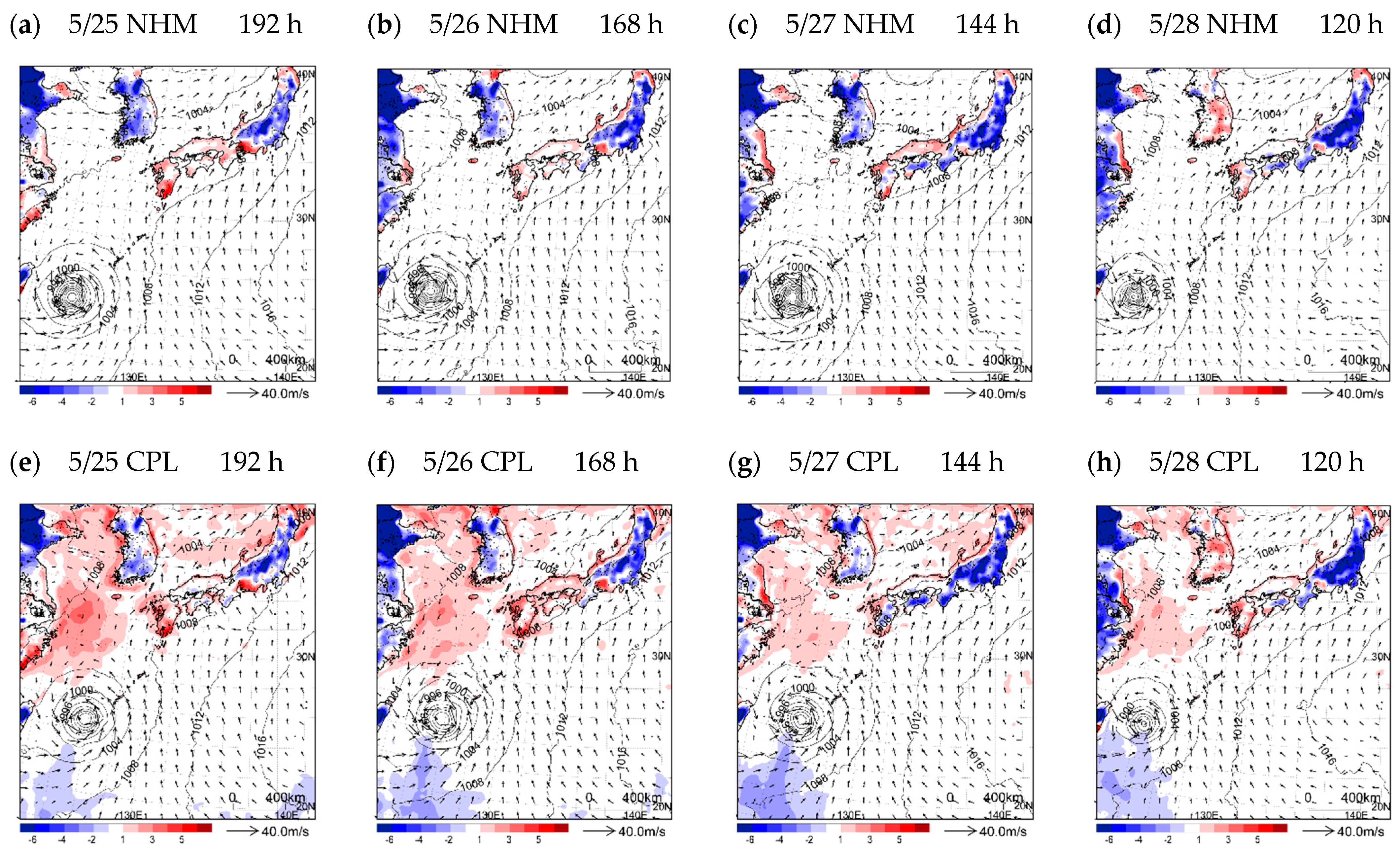
3.2. Simulation Results by a Regional Model

Section 3.1 shows that the differences in models between the JMA and NCEP and the initial times, i.e., differences in the initial atmospheric conditions, had an impact on the Mawar predictions and the location of the front along the southern coast of Japan. This section shows the results of numerical simulations under four initial conditions for which the initial time was 00 UTC on 25–28 May in 2023 using the NHM and CPL [13]. In fact, the physical processes in the NHM and the atmospheric part of the CPL (Table 2) were different from those of the JMA global model [28]. The other reason for the simulations by the CPL was that the time evolution of Mawar’s central pressure predicted by the JMA global model showed the deepening of the central pressure, even in the decaying phase when the central pressure in the preliminary analysis was rising (Figure 3). Since the horizontal resolution of 3 km in the NHM and CPL (Table 3) was finer than that of the JMA global model, 13 km (Table 1), it is inferred that the time evolution of the central pressure simulated by the NHM could show the deepening in a similar way. The aim of this section is to verify the extent to which the excess deepening in the decaying phase was suppressed by the effects of ocean coupling and the extent to which it affected the track prediction for Mawar.
Figure 8a shows the horizontal distribution of Mawar’s track simulations with the track obtained from the RSMC Tokyo preliminary analysis. The dates displayed in Figure 8a indicate the position of Mawar in the preliminary analysis at the corresponding date. The northwestward translation in an earlier integration time for all simulations was consistent with the results of the preliminary analysis. However, excessive northwestward translation was also found in all simulations. The result is consistent with the prediction by the JMA global model. Figure 8b shows the timeseries of Mawar’s central pressure predictions in all simulations, along with the timeseries of central pressure in the preliminary analysis. The central pressures at the initial time tended to be high compared to that in the early analysis, because those were created from the analysis based on the JMA global-model system. The effect of ocean coupling on the central pressure simulations began to appear at an earlier integration time. The excessive deepening of the central pressure simulated by the NHM from the initial time to 96 h was suppressed by the CPL. Therefore, the decay rate of central pressures simulated by the CPL was more consistent with the preliminary analysis than that simulated by the NHM. It should be noted that the effect of ocean coupling on the track simulations was minor compared to that on the central pressure simulations. Although these are only results simulated by a regional model for one case study, ocean coupling can improve the intensity prediction without significantly affecting the track prediction. The result is consistent with previous studies that used an atmosphere–ocean coupled model [13,19,29,30,31].
Figure 9 shows the horizontal map of the difference in surface temperatures (both SST and ground temperature) from the initial time to 00 UTC on 2 June with SST values at the initial time of the numerical simulation. There was no difference in the SSTs predicted by the NHM, while the ground temperature clearly showed the difference, since the ground temperature was predicted in the NHM [9]. Around the simulated Mawar, sea surface cooling induced by Mawar was simulated by the CPL. Although the amplitude was slightly different between the four simulations, the location of simulated sea surface cooling was consistent with the analysis using the OISST products (Figure 10). It should be noted that the SSTs over the East China Sea and the Sea of Japan were rising during the analysis period. The rising SSTs were reasonably simulated by the CPL. However, the rising SSTs around the Subtropical High and decreasing SSTs along the Kuroshio path could not be successfully simulated. In particular, Kuroshio was meandering off the Kii peninsula (Figure 1a) and the areas of decreasing SST from the initial time were distributed along the Kuroshio path.
Figure 11 shows the horizontal distribution of the precipitation amount summed from 00 UTC on 1 June to 2300 UTC on 2 June in 2023. The contours in Figure 11 show the horizontal map of the simulated sea-level pressure. The horizontal distribution of the summed precipitation around Mawar simulated by the NHM showed precipitation maxima in the east and west with respect to the track of Mawar, whereas that simulated by the CPL showed maxima only in the east. The asymmetric distribution simulated by the CPL is partly due to the atmospheric response to a decrease in the sea surface temperature (SST) caused by Mawar [13,31]. As shown in Figure 5, the difference in Mawar’s predictions between the initial times and between the NHM and CPL is related to the difference in the summed precipitation where Mawar was traveling. It should also be noted that an asymmetric precipitation pattern was noticeable when the moving speed of the simulated Mawar was relatively fast.
In each experiment, the band-like heavy rainfall area over the front along the southern coast of Japan was more realistically simulated than the results of the global model products (Figure 5). Even though the JMA global model products were used to create the initial and lateral boundary conditions for the eight numerical simulations (Table 3), the northeastward movement of Mawar after the recurvature in the preliminary analysis was relatively slow in the NHM and CPL simulations, irrespective of the initial time compared with that predicted by the JMA global model (Figure 2). The slow northeastward translation of the simulated Mawar would be related to the location of the band-like heavy rainfall area over the front. Therefore, the differences in Mawar’s track predicted by the JMA global model and those in the location of the band-like heavy rainfall area over the front were not noticeable in the results of simulations by the NHM and the CPL between the initial times on 25 and 28 May.
Figure 12 shows the horizontal map of moisture flux at a height of 1470 m, corresponding to the 13th vertical level of NHM and CPL and approximately the 850 hPa level at 00 UTC on 2 June. Moisture fluxes exceeding 500 g m−2 s−1 were found within the inner core of the simulated Mawar. On the eastern side of the simulated Mawar, the broad area of moisture transport from 22° N (corresponding to the latitude of the location of Mawar) to 34° N (corresponding to the latitude of the front along the southern coast of Japan) was formed as a moisture road on a length scale of approximately 1000 km. Although the amount of moisture flux over the moisture road varied depending on the initial time and whether the regional model used for the simulation was the NHM or CPL, the location of the moisture road as well as the location of the band-like heavy rainfall area (Figure 11) was not changed in all simulations. In Figure 5, the horizontal winds at an 850 hPa level show that the location of the band-like heavy rainfall area was associated with that of moisture road. When the initial time was 00 UTC on 25 May, the moisture road could be predicted by the JMA and NCEP global models, although the location of the front shifted eastward to some extent due to the eastward location of the predicted Mawar and the associated moisture road. However, the moisture road could not be predicted by the NCEP global model when the initial time was 00 UTC on 28 May (Figure 5). A broad rainband extending northeastward from the southern side of the predicted Mawar was separated from the inner core of the simulated typhoon. This suggests that only the broad rainband may have formed as an atmospheric river that played a crucial role in supplying moist air to the band-like heavy rainfall area over the front, irrespective of the location of Mawar. Such a separation found in the NCEP global model products, however, has not been simulated by the NHM and CPL. With respect to factors that fundamentally affect the atmospheric environments on a synoptic scale, it is beyond the scope of this study.

3.3. Mechanisms of TC Motion and Heavy Rainfall

Section 3.2 showed that the accurate track simulations of Mawar and the moisture road oriented from the east of Mawar were important for predicting the location of the front along the southern coast of Japan where heavy rainfall occurred (Figure 1a). In addition, Section 3.2 showed the effects of ocean coupling and the atmospheric initial conditions on the prediction of the moisture road. This section addresses the relationship between Mawar’s track and the structural change in the simulated inner core of Mawar caused by the ocean coupling. Moreover, this study investigates the effect of ocean coupling on the formation mechanism of the moisture road using the results of numerical simulations conducted by the NHM and CPL at which the initial time was 00 UTC on 28 May in 2023.
Figure 13a shows the horizontal wind field at a height of 1470 m simulated by the NHM at 06 UTC on 2 June (126 h from the initial time). A dashed line in Figure 13a shows the location of the cross section that represents the vertical profile of Ertel’s potential vorticity (PV) [32], the potential temperature, and the horizontal and vertical wind vectors along the line (Figure 13b). The horizontal wind field shows that wind speeds exceeding 17 m s−1 were simulated over the moisture road. The vertical section across the center of the simulated Mawar indicates that the thickness of the moisture road was thicker than 4 km. The positive potential vorticity was upright around Mawar’s position with peaks at the 3 km and 11 km heights, respectively. At 126 h, there was no effect of the meandering of westerlies in the upper troposphere on the simulated Mawar structure. Mawar simulated by the NHM was actually moving to the northeast more slowly than that simulated by the CPL.
The horizontal wind field simulated by the CPL showed asymmetry within the inner core of the simulated Mawar (Figure 13c). This is due to the negative impact caused by sea surface cooling (Figure 9). The ocean coupling also affected the value of PV within the inner core (Figure 13d). In the lower troposphere, the PV tower defined by a positive potential vorticity of higher than 10−6 m2 s−1 K kg−1 [33] was tilted northeastward, while in the upper troposphere, it was tilted southwestward above a height of approximately 7 km. Since the height of the upright PV tower became relatively low in the decaying phase, the steering flows that affected the movement of the simulated Mawar could be determined only by the southwesterly flow in the lower troposphere. Therefore, in addition to the increase in the simulated central pressure due to oceanic coupling, the lowering of the height of the PV tower in the inner core could have further accelerated its northeastward movement. After 126 h, as shown in Figure 6, the interaction with the mid-latitudes may have accelerated the northeastward motion, and then a phase transition to extratropical cyclone occurred while Mawar was traveling northeastward.
Figure 14a shows the horizontal distribution of the moisture flux at the 1470 m height simulated by the NHM at 06 UTC on 2 June. The moisture flux exceeded 500 kg m−2 s−1 around the simulated Mawar, which was distributed symmetrically, centered at the predicted Mawar location. A dashed line in Figure 14a was used to investigate the vertical profile of the moisture flux along the moisture road. The height of the moisture road at the location of the cross section ranged from 3 km to just under 6 km (Figure 14b). The moisture flux showed its maximum value around the 500 m height around the front along the southern coast of Japan, and the amount was greater than the moisture flux east of the simulated Mawar. The effect of ocean coupling was clearly found in the asymmetric distribution of the moisture flux around the simulated Mawar (Figure 14c), which was different from the symmetric distribution simulated by the NHM (Figure 14a). The asymmetry was consistent with the distribution of the summed precipitation amount shown in Figure 11. However, the height of the moisture road and its tendency for the moisture fluxes to increase toward the front along the southern coast of Japan were similar to those simulated by the NHM (Figure 14b,d). The difference in the SST simulated by the CPL from the initial time was not significant (Figure 9). This is one of the reasons why the effect of ocean coupling on the moisture flux over the moisture road was not noticeable.
To investigate the factors contributing to the southerlies between the simulated Mawar and the Subtropical High, particularly the formation of the moisture flux maxima at a height of 500 m, the pressure gradient along the x-axis was addressed to investigate the contribution of the pressure gradient force to the meridional flow over the moisture road. Figure 15a shows the horizontal distribution of the pressure gradient along the x-axis at a height of 500 m at 06 UTC on 2 June. The location of the cross-section line is the same as in Figure 14a. The pressure gradient locally increased east of the simulated Mawar and near the southern coast of Japan (Figure 15b), suggesting that the increases in the southerlies were caused by local convection, partly forced by the orographic effect along the southern coast of Japan. However, the southerly component was also prominent at the locations where the pressure gradient was relatively small, suggesting a possible contribution from the marginal flow of the Subtropical High. In other words, the moisture road is caused by a combination of the marginal flow around the western edge of the Subtropical High with the enhanced pressure gradient due to local convection.
Although the effect of oceanic coupling on the pressure gradient appeared around the simulated Mawar due to the differences in the simulated central pressures, this study focuses here on the difference in the local pressure gradient between the simulated Mawar and the Subtropical High. The pressure gradient simulated by the CPL locally increased within a spiral band pattern east of the simulated Mawar compared with the result simulated by the NHM (Figure 15c,d). However, the increase in the pressure gradient along the southern coast of Japan was reduced due to ocean coupling (Figure 15d) when it was compared with the pressure gradient simulated by the NHM (Figure 15b). Regardless of the differences in the pressure gradients between the NHM and CPL, the effect of ocean coupling on the moisture flux over the moisture road was small, except east of the simulated Mawar. This suggests that the moisture road was primarily influenced by the marginal flow around the Subtropical High rather than by the location of the simulated Mawar and ocean coupling.

4. Discussion

Previous studies involving a regional atmosphere–ocean coupled model reported that the impact of ocean coupling on TC track predictions is small [13,19,29,30,31]. However, the regional atmosphere–ocean coupled model used in the previous studies used a horizontal resolution of finer than 10 km to investigate the detailed structure of the inner core and the structural and intensity changes, so the integration time was usually shorter than 5 days. This study differs from previous studies in that it addresses the predictability of not only Mawar’s inner-core structure but also the predictability of a remote heavy-rainfall event far from Mawar after 5 days. In addition, the study of TC–ocean interactions for Mawar is unique in that Mawar was in the early rainy season from late May to early June. To the best of the author’s knowledge, this is the first attempt to study the indirect effects of TCs and air–sea interactions on the formation of the front along the southern coast of Japan through moisture transport over the moisture road during the early summer rainy season. If the horizontal resolution of the regional atmosphere–ocean coupled model was finer, it might be possible to quantitively predict the localized stationary heavy rainfall events over the quasi-stationary front.
A global atmosphere–ocean coupled model has already been developed by ECMWF [34] and UKMet [35] (Table 1). Although TC cases are limited in terms of verification, there is a certain effect of ocean coupling on the TC intensity prediction, but this is neutral with respect to the TC track prediction. While the present study was able to simulate not only the decrease in the SST induced by Mawar but also the increases in the Sea of Japan and the East China Sea, it was not able to simulate the decrease in the SSTs from the initial times along the Kuroshio path and the increase in the SSTs from the initial time around the Subtropical High (Figure 9 and Figure 10). These two issues need to be discussed separately. As for the former issue, a three-dimensional ocean model is required to simulate the decrease in the SSTs from the initial time along the Kuroshio path. This cannot be simulated in a multilayer ocean model incorporated into the CPL. In fact, horizontal advection as well as turbulent mixing and upwelling induced by TCs plays a crucial role in determining the variation in SSTs caused by passage of a TC, particularly with a moving speed of slower than 3 m s−1 [36]. In the latter issue, the atmospheric physical processes in the NHM (Table 2) should be improved to realistically simulate the cloud distribution to obtain a more realistic distribution of the solar radiation. When clouds are excessively simulated around the Subtropical High, solar radiation is reduced and consequently suppresses the increase in the simulated SST during the day [37].
This study suggests that the improvement of the simulation of the Subtropical High leads to improvements in not only the prediction of SSTs but also the reproducibility of the locations of the moisture road and the quasi-stationary front along the southern coast of Japan. This means that the improvements in both the initial condition and the prediction of the Subtropical High by the global model not only improve the TC track prediction after five days but also enhance the predictability of the heavy rainfall over the front on local to synoptic scales. In order to accurately predict the moisture road, it is important to accurately predict the locations of the Subtropical High and the tropical depression or the monsoon gyre [38] west of the Subtropical High, irrespective of the TC intensity involved in the gyre.
This study reconfirms that ocean coupling is effective for predicting the TC intensity [13,19,29,30,31]. Especially in the case of TCs during the early summer rainy season, this study represents the first attempt to study TC–ocean interactions in a broader view from a mesoscale scale to a synoptic one. The impact of ocean coupling on the TC track prediction shown in Figure 8a seems to be minor when considering the large differences among the global models (Figure 2), although the northeastward translation was more clearly simulated by the CPL (Figure 8a). This suggests that the coupled atmosphere–ocean modeling for global atmosphere models will be able to improve the TC intensity predictions without significantly compromising the performance of the TC track predictions. However, improvements in atmospheric physical processes and initial conditions in a global forecast system could affect both the TC track and the intensity predictions. This is beyond the scope of this study and is a subject for future work.

5. Conclusions

While Typhoon Mawar was moving northeastward south of Japan after the recurvature in 2023, a localized stationary heavy rainfall event occurred over the quasi-stationary front along the southern coast of Japan on 1–2 June during the early summer rainy season. Although the global model predictions by four major global models (ECMWF, NCEP, JMA, UKMet) appeared to have small errors when Mawar was moving northwestward, the predicted Mawar actually moved more slowly than the result of the RSMC Tokyo preliminary analysis, irrespective of the difference in the initial time. Moreover, the predicted Mawar tended to move further northwestward around the recurvature area with slow translation so that the spread of the predicted Mawar track became broader after the recurvature than before. In fact, it was difficult to predict Mawar’s track after the recurvature, and as a result, there was a great deal of uncertainty regarding the prediction of heavy rainfall over the front along the southern coast of Japan after five days.
First, the atmospheric environments surrounding the predicted Mawar were investigated by using the NCEP and JMA global model products that were available. The results of the JMA global products suggested that the JMA model could predict the location of the front along the southern coast of Japan on 1–2 June better than the NCEP model, since the Mawar track predicted by the JMA global model was more consistent with the RSMC Tokyo preliminary analysis, even after 5 days.
During the passage of Mawar, the horizontal distribution of the daily SST shows variations, such as the sea surface cooling induced by Mawar and along the Kuroshio path and the increases in SSTs over the East China Sea, the Sea of Japan, and around the Subtropical High. In particular, a noticeable decrease in the SST was analyzed south of the recurvature area where the predicted Mawar in the JMA global model products showed overdevelopment. In order to clarify the contribution of the sea surface cooling to the prediction of Mawar and the location of the quasi-stationary front along the southern coast of Japan, numerical simulations were performed by the NHM and CPL. Regardless of the initial time used in the numerical simulation, the central pressures predicted by the CPL were more consistent with the preliminary analysis than those predicted by the NHM with regard to two respects: the suppression of overdevelopment in an earlier integration time and the values of the central pressure in the decaying phase of Mawar.
With respect to the track prediction, the CPL predicted a more northeastward translation than the NHM. The upright structure of the positive PV in the inner core simulated by the NHM was separated into two parts in the lower troposphere and the upper troposphere, respectively, when the CPL was used for Mawar’s simulations. Since southwesterly winds were dominant as a steering flow in the lower troposphere, the relatively low vortex with a positive PV simulated by the CPL tended to move further northeastward than that by the NHM.
The area of moisture transport between Mawar and the Subtropical High was distributed on a length scale of approximately 1000 km and a height scale of 4 km, which was consistent with the characteristics of the moisture road [4]. With respect to the formation of southerly winds over the moisture road, the effect of ocean coupling on the pressure gradient along the x-axis was noticeable east of the simulated Mawar and over the front along the southern coast of Japan due to the enhancement of local convection. However, the marginal flow around the Subtropical High played a major role in the formation of moisture roads. In other words, not only ocean coupling but also Mawar’s intensity were found to play minor roles in the formation of the moisture road. The eastward shift in the location of the Subtropical High predicted by the NCEP global model did affect the unrealistic location of the front predicted far from the southern coast of Japan by shifting the location of the moisture road eastward, even if it was no longer associated with the movement of the predicted Mawar. The relationship between the eastward retreat of the Subtropical High and the global model specification in the JMA and NCEP global models is beyond the scope of this study. When considering the effect on the atmospheric environments of ocean coupling represented by the variations in SSTs, particularly the sea surface cooling induced by Mawar, this study suggests that the application of a global atmosphere–ocean coupled model to a numerical forecast system will be effective for improving the TC intensity predictions without having a significant impact on the TC track predictions. However, it remains to be seen whether the interrelationships between TCs and the ocean and atmospheric environments demonstrated in this study can be applied to the TC predictions for other TC cases and other seasons.

Funding

This research was funded by Grants-in-Aid for Scientific Research JP22K03725.

Institutional Review Board Statement

Not applicable.

Informed Consent Statement

Not applicable.

Data Availability Statement

Some of the data sets and program codes used in this study are not publicly available due to the management policy of the Japan Meteorological Agency (JMA) but may be available from the first author for reasonable usage upon request. All rights remain with JMA.

Acknowledgments

The author appreciates the anonymous reviewers for their comments which helped to improve the first manuscript. Generic Mapping Tools software version 5.4.5 (https://www.soest.hawaii.edu/gmt/ (accessed on 15 September 2023)) was used to draw the figures.

Conflicts of Interest

The author declares no conflict of interest.

References

  1. Makihara, Y. A method for improving radar estimates of precipitation by comparing data from radars and raingauges. J. Meteorol. Soc. Jpn. 1996, 74, 459–480. [Google Scholar] [CrossRef]
  2. Yoshida, N.; Kawamura, R.; Kawano, T.; Mochizuki, T.; Iizuka, S. Remote dynamic and thermodynamic effects of typhoons on Meiyu–Baiu precipitation in Japan assessed with bogus typhoon experiments. Weather Clim. Extrem. 2023, 41, 100578. [Google Scholar] [CrossRef]
  3. Kodama, S.; Satoh, M. Statistical analysis of remote precipitation in Japan caused by typhoons in September. J. Meteorol. Soc. Jpn. 2022, 100, 893–911. [Google Scholar] [CrossRef]
  4. Yoshida, K.; Ito, H. Indirect effects of tropical cyclones on heavy rainfall events in Kyushu, Japan, during the Baiu season. J. Meteorol. Soc. Jpn. 2012, 90, 377–401. [Google Scholar] [CrossRef]
  5. Schumacher, R.S.; Galarneau, T.J.; Bosart, L.F. Distant effects of a recurving tropical cyclone on rainfall in a midlatitude convective system: A high-impact predecessor rain event. Mon. Weather Rev. 2011, 139, 650–667. [Google Scholar] [CrossRef]
  6. Knippertz, P.; Martin, J.E. A pacific moisture conveyor belt and its relationship to a significant precipitation event in the semiarid southwestern united states. Weather Forecast 2007, 22, 125–144. [Google Scholar] [CrossRef]
  7. American Meteorological Society. Atmospheric River. Glossary of Meteorology. Available online: http://glossary.ametsoc.org/wiki/Atmospheric_river (accessed on 15 September 2023).
  8. THORPEX Interactive Grand Global Ensemble (TIGGE) Model Tropical Cyclone Track Data. Available online: https://rda.ucar.edu/datasets/ds330.3/dataaccess/ (accessed on 15 September 2023).
  9. Ikawa, M.; Saito, K. Description of a nonhydrostatic model developed at the forecast research department of the MRI. Tech. Rep. MRI 1991, 28, 238. [Google Scholar] [CrossRef]
  10. Lin, Y.L.; Farley, R.D.; Orville, H.D. Bulk parameterization of the snow field in a cloud model. J. Appl. Meteorol. Climatol. 1983, 22, 1065–1092. [Google Scholar] [CrossRef]
  11. Kondo, J. Air-sea bulk transfer coefficients in diabatic conditions. Bound.-Layer Meteorol. 1975, 9, 91–112. [Google Scholar] [CrossRef]
  12. Taylor, P.K.; Yelland, M.J. The dependence of sea surface roughness on the height and steepness of the waves. J. Phys. Oceanogr. 2001, 31, 572–590. [Google Scholar] [CrossRef]
  13. Wada, A.; Kanada, S.; Yamada, H. Effect of air-sea environmental conditions and interfacial processes on extremely intense typhoon Haiyan (2013). J. Geophys. Res. 2018, 123, 10379–10405. [Google Scholar] [CrossRef]
  14. Klemp, J.B.; Wilhelmson, R. The simulation of three-dimensional convective storm dynamics. J. Atmos. Sci. 1978, 35, 1070–1096. [Google Scholar] [CrossRef]
  15. Deardorff, J.W. Stratocumulus-capped mixed layers derived from a three-dimensional model. Bound.-Layer Meteorol. 1980, 18, 495–527. [Google Scholar] [CrossRef]
  16. Sugi, M.; Kuma, K.; Tada, K.; Tamiya, K.; Hasegawa, N.; Iwasaki, T.; Yamada, S.; Kitade, T. Description and performance of the JMA operational global spectral model (JMA-GSM88). Geophys. Mag. 1990, 43, 105–130. [Google Scholar]
  17. Saito, K. The JMA nonhydrostatic model and its applications to operation and research. In Atmospheric Model Applications; Yucel, I., Ed.; InTech: Houston, TX, USA, 2012; pp. 85–110. [Google Scholar] [CrossRef]
  18. Japan Meteorological Agency. Outline of the operational numerical weather prediction at the Japan Meteorological Agency. In Appendix to WMO Technical Progress Report on the Global Data-Processing and Forecasting System (GDPFS) and Numerical Weather Prediction (NWP) Research; Japan Meteorological Agency: Tokyo, Japan, 2013; 201p. [Google Scholar]
  19. Bender, M.A.; Ginis, I.; Kurihara, Y. Numerical simulations of tropical cyclone-ocean interaction with a high-resolution coupled model. J. Geophys. Res. 1993, 98, 23245–23263. [Google Scholar] [CrossRef]
  20. Schiller, A.; Godfrey, J.S. A diagnostic model of the diurnal cycle of sea surface temperature for use in coupled ocean-atmosphere models. J. Geophys. Res. 2005, 110, C11014. [Google Scholar] [CrossRef]
  21. Ohlmann, J.C.; Siegel, D.A. Ocean radiant heating. Part II: Parameterizing solar radiation transmission through the upper ocean. J. Phys. Oceanogr. 2000, 30, 1849–1865. [Google Scholar] [CrossRef]
  22. Remote Sensing Systems Measurement Sea Surface Temperature. Available online: https://www.remss.com/measurements/sea-surface-temperature/ (accessed on 15 September 2023).
  23. Usui, N.; Wakamatsu, T.; Tanaka, Y.; Hirose, N.; Toyoda, T.; Nishikawa, S.; Fujii, Y.; Takatsuki, Y.; Igarashi, H.; Nishikawa, H.; et al. Four–dimensional variational ocean reanalysis: A 30–year high–resolution dataset in the western North Pacific (FORA–WNP30). J. Oceanogr. 2017, 73, 205–233. [Google Scholar] [CrossRef]
  24. Wada, A.; Chan, J.C.L. Increasing TCHP in the western North Pacific and its influence on the intensity of FAXAI and HAGIBIS in 2019. SOLA 2021, 17A, 29–32. [Google Scholar] [CrossRef]
  25. Chan, J.C.L. The physics of tropical cyclone motion. Annu. Rev. Fluid Mech. 2005, 37, 99–128. [Google Scholar] [CrossRef]
  26. Kobayashi, S.; Kosaka, Y.; Chiba, J.; Tokuhiro, T.; Harada, Y.; Kobayashi, C.; Naoe, H. JRA-3Q: Japanese Reanalysis for Three Quarters of a Century. In Proceedings of the Joint WCRP-WWRP Symposium on Data Assimilation and Reanalysis/ECMWF Annual Seminar 2021, Online, 16 September 2021. [Google Scholar]
  27. Hersbach, H.; Bell, B.; Berrisford, P.; Hirahara, S.; Horányi, A.; Muñoz-Sabater, J.; Nicolas, J.; Peubey, C.; Radu, R.; Schepers, D.; et al. The ERA5 global reanalysis. Q. J. R. Meteorol Soc. 2020, 146, 1999–2049. [Google Scholar] [CrossRef]
  28. Yonehara, H.; Kuroki, Y.; Ujiie, M.; Matsukawa, C.; Kanehama, T.; Nagasawa, R.; Ochi, K.; Higuchi, M.; Ichikawa, Y.; Sekiguchi, R.; et al. Upgrade of JMA’s operational global numerical weather prediction system. WGNE Res. Activ. Earth Syst. Modell. 2023, 53, 6-15–6-16. [Google Scholar]
  29. Bender, M.A.; Ginis, I. Real-case simulations of hurricane–ocean interaction using a high-resolution coupled model: Effects on hurricane intensity. Mon. Weather Rev. 2000, 128, 917–946. [Google Scholar] [CrossRef]
  30. Ito, K.; Kuroda, T.; Saito, K.; Wada, A. Forecasting a large number of tropical cyclone intensities around Japan using a high-resolution atmosphere–ocean coupled model. Weather Forecast 2015, 30, 793–808. [Google Scholar] [CrossRef]
  31. Wada, A.; Uehara, T.; Ishizaki, S. Typhoon-induced sea surface cooling during the 2011 and 2012 typhoon seasons: Observational evidence and numerical investigations of the sea surface cooling effect using typhoon simulations. Prog. Earth Planet. Sci. 2014, 1, 11. [Google Scholar] [CrossRef]
  32. Davis, C.A.; Emanuel, K.A. Potential vorticity diagnostics of cyclogenesis. Mon. Weather Rev. 1991, 119, 1929–1953. [Google Scholar] [CrossRef]
  33. Wada, A.; Yanase, W.; Okamoto, K. Interactions between a tropical cyclone and upper-tropospheric cold-core lows simulated by an atmosphere-wave-ocean coupled model: A case study of Typhoon Jongdari (2018). J. Meteorol. Soc. Jpn. 2022, 100, 387–414. [Google Scholar] [CrossRef]
  34. Mogensen, K.S.; Magnusson, L.; Bidlot, J.-R. Tropical cyclone sensitivity to ocean coupling in the ECMWF coupled model. J. Geophys. Res. Ocean. 2017, 122, 4392–4412. [Google Scholar] [CrossRef]
  35. Met Office Numerical Weather Prediction Models. Available online: https://www.metoffice.gov.uk/research/approach/modelling-systems/unified-model/weather-forecasting (accessed on 15 September 2023).
  36. Yablonsky, R.M.; Ginis, I. Limitation of one-dimensional ocean models for coupled hurricane-ocean model forecasts. Mon. Weather Rev. 2009, 137, 4410–4419. [Google Scholar] [CrossRef]
  37. Kawai, Y.; Wada, A. Diurnal sea surface temperature variation and its impact on the atmosphere and ocean: A review. J. Oceanogr. 2007, 63, 721–744. [Google Scholar] [CrossRef]
  38. American Meteorological Society. Monsoon Gyre. Glossary of Meteorology. Available online: https://glossary.ametsoc.org/wiki/Monsoon_gyre (accessed on 15 September 2023).
Figure 1. (a) Horizontal distribution of the radar–rain gauge analyzed precipitation amount summed every 10 min from 0000 UTC on 1 June to 2350 UTC on 2 June in 2023. A solid line with circles indicates the track of Mawar. The labels indicate the time at the location of Mawar based on the preliminary analysis. (b) Weather map at 00 UTC on 2 June in 2023.
Atmosphere 14 01638 g001
Figure 2. (a) Horizontal map of the track predictions for 168 h every 12 h (triangles plotted every 24 h) at which the initial time was 00 UTC from 25 to 28 May in 2023, together with the positions of the early analysis (black circles with a solid line) every 12 h. (b) Same as (a), but the map is focused on around the recurvature of Mawar. The color bars indicate the values of the central pressure (hPa) at the location of the predicted Mawar. Data sources (the abbreviation of institute) are indicated by colors such as red, blue, violet, and green.
Atmosphere 14 01638 g002
Figure 3. Timeseries of the predicted central pressures every 12 h at which the initial time was 00 UTC from 25 to 28 May in 2023. Data sources are indicated by colors such as red (JMA), blue (ECMWF/EC), green (NCEP), and violet (UKMet/UK). The results of preliminary analysis by RSMC Tokyo are shown by a black line.
Atmosphere 14 01638 g003
Figure 4. Computational domain used for the numerical simulations conducted by the NHM and CPL.
Atmosphere 14 01638 g004
Figure 5. Horizontal distribution of the predicted precipitation amount summed every 6 h from 00 UTC on 1 June to 00 UTC on 3 June in 2023. The arrows indicate predicted winds exceeding 10 ms−1 at an 850 hPa level at 00 UTC on 2 June in 2023. The red circles indicate the position of the predicted Mawar at 00 UTC on 2 June in 2023. The upper panels show the JMA’s predictions at which the initial times are (a) 00 UTC on 25 May and (b) 00 UTC on 28 May. The lower panels show the NCEP’s predictions at which the initial times are (c) 00 UTC on 25 May and (d) 00 UTC on 28 May.
Atmosphere 14 01638 g005
Figure 6. The same as Figure 5, except for the horizontal distribution of the predicted height of the 500 hPa level (dashed contour) and that of the predicted horizontal winds exceeding 15 ms−1 (red vectors) at the 300 hPa level at 00 UTC on 2 June in 2023. The blue circles indicate the positions of the predicted Mawar from each initial time. The larger circles indicate the locations of the predicted Mawar at 00 UTC on 2 June. The dashed contour interval is 40 m.
Atmosphere 14 01638 g006
Figure 7. The same as Figure 6 except for the horizontal distribution from the (a) JRA-3Q and (b) ERA5 reanalysis data sets.
Atmosphere 14 01638 g007
Figure 8. (a) Horizontal map of track predictions every 12 h at which the initial time was 00 UTC from 25 to 28 May in 2023. The colors within the circles indicate the values of the early analyzed (squares) and predicted central pressures (circles). (b) Timeseries of the predicted central pressures every 12 h at which the initial time was 00 UTC from 25 to 28 May in 2023 with the timeseries of the preliminary analysis (black circles). Line colors with open circles indicate the model used (red, NHM, blue, CPL).
Atmosphere 14 01638 g008
Figure 9. Horizontal maps of the difference in the surface temperature with surface winds at 00 UTC on 2 June in 2023 from the initial time. The upper panels (ad) show the results simulated by the NHM, while the lower panels (eh) show the results simulated by the CPL. In the results of the simulations conducted by the NHM, only the ground temperature was changed. The initial time is 00 UTC on (a,e) 25, (b,f) 26, (c,g) 27, and (d,h) 28 in May (from the left to the right side).
Atmosphere 14 01638 g009
Figure 10. Horizontal maps of the difference in the SST on June 2 in 2023 from (a) 25, (b) 26, (c) 27, and (d) 28 May with the solid contour indicating the SST distribution (a) 25, (b) 26, (c) 27 and (d) 28 May in the OISST products. Red (blue) indicates the rise (decrease) in the SST. The contour interval is 1 °C.
Atmosphere 14 01638 g010
Figure 11. The same as Figure 9, except for the precipitation amount summed from 00 UTC on 1 June to 2300 UTC on 2 June in 2023 with sea-level pressures (contours) and surface winds at 23 UTC on 2 June. Magenta circles with solid lines indicate the simulated track every 24 h from 00 UTC on 1 June to 0000 UTC on 3 June.
Atmosphere 14 01638 g011
Figure 12. The same as Figure 9, except for the horizontal moisture flux at a height of 1470 m (the 13th vertical level) at 00 UTC on 2 June.
Atmosphere 14 01638 g012
Figure 13. (a) Horizontal distribution of the sea-level pressure and wind velocity at the 1470 m height (13th level) with wind vectors at 126 h simulated by the NHM. The dashed purple line indicates the location of the cross section. (b) The vertical cross section along the line indicates the PV profiles (shades: 1 PV unit = 10−6 m2 s−1 K kg−1) with horizontal–vertical winds along the line. (c,d) The same as (a,b) except for the CPL. The double lines in (b,d) indicate the slope of the simulated Mawar vortex represented by the values of the potential temperature.
Atmosphere 14 01638 g013
Figure 14. The same as Figure 13, except for (a,c) moisture fluxes at a height of 1470 m (13th level) and (b,d) moisture fluxes (kg m−2 s−1).
Atmosphere 14 01638 g014
Figure 15. The same as Figure 13, except for (a,c) pressure gradients in an x-axis at a height of 500 m and (b,d) the zonal pressure gradient (hPa dx−1). ‘dx’ indicates a grid resolution (3 km in this study) on the x-axis.
Atmosphere 14 01638 g015
Table 1. List of four global model specifications used in this study included in the TIGGE data set.
ECMWFJMANCEPUKMet
Model (Atmosphere)Integrated Forecasting System (IFS) Cycle 47r3
Global Spectral ModelGlobal Forecast System Forecast System v16.3Unified model Operational Suite Cycle 45
Model (Ocean)Nucleus for European Modelling of the Ocean (NEMO) Nucleus for European Modelling of the Ocean (NEMO)
SST Merged Satellite and In-situ Data Global Daily Sea Surface Temperature (MGDSST)Near-Surface Sea Temperature (NSST)
Model (Wave)High RESolution WAve Model (HRES-WAM)
Horizontal resolution and Vertical level (Atmosphere)~9 km
(Top 0.01 hPa)
Tco1279L137
~13 km
(Top 0.01 hPa)
TQ959L128
13 km L127
(Top 80 km)
10 km L70
(Top 80 km)
Horizontal resolution (Ocean)28 km0.25 degrees1/12 degrees0.25 degrees
Forecast time at 00 UTC10 days11 days16 days7 days
Table 2. Experiment name and physics model used in the atmosphere and air–sea interface.
NHMCPL
ModelA nonhydrostatic atmosphere modelCoupled atmosphere–wave–ocean model
MicrophysicsIkawa and Saito (1991) [9], Lin et al. (1983) [10].
Surface fluxKondo (1975) [11]Taylor and Yelland (2001) [12],
Wada et al. (2018) [13]
TurbulenceKlemp and Wilhelmson (1978) [14], Deardorff (1980) [15]
RadiationSugi et al. (1990) [16]
Table 3. Configuration used in each experiment.
NHMCPL
Initial and integration timesFrom 00 UTC on 25, 26, 27, 28 May to 00 UTC on 4 June in 2023
Time step6 s6 s (Atmosphere),
36 s (Ocean),
6 min (Ocean wave)
Computational domain and map system4500 km (zonal) and 4320 km (meridional) centered at 25° N, 137° E, Lambert Conformal Conic projection
Horizontal resolution and vertical layer3 km and 55 levels in vertical coordinates with intervals ranging from 40 m for the near-surface layer to 1180 m for the uppermost layer (top height is 27,440 m)
Initial data for SSTDaily microwave sea surface temperature on 24, 25, 26, and 27 May in 2023 (1 day before the initial time)
Initial and boundary conditions for the ocean model (temperature, salinity, and current velocities)-JMA mean North Pacific oceanic daily analysis on 24, 25, 26, and 27 May in 2023
Initial and boundary conditions for the atmosphere modelJMA 6 hourly global model products with a horizontal grid spacing of approximately 10 km
Disclaimer/Publisher’s Note: The statements, opinions and data contained in all publications are solely those of the individual author(s) and contributor(s) and not of MDPI and/or the editor(s). MDPI and/or the editor(s) disclaim responsibility for any injury to people or property resulting from any ideas, methods, instructions or products referred to in the content.

