Article

Effect of Source Emission Control Measures on Source of Atmospheric PM2.5 during “Parade Blue” Period

Department of Building Environment and Energy Engineering, School of Civil and Resources Engineering, University of Science and Technology Beijing, Beijing 100083, China
*
Author to whom correspondence should be addressed.
Atmosphere 2023, 14(11), 1639; https://doi.org/10.3390/atmos14111639
Submission received: 25 September 2023 / Revised: 19 October 2023 / Accepted: 30 October 2023 / Published: 31 October 2023
(This article belongs to the Section Aerosols)

Abstract

:
During the “Parade Blue” period in 2015, Beijing and its surrounding areas implemented mandatory temporary source control strategies, which provided experimental conditions for studying the effects of source emission control measures on the sources of atmospheric PM2.5. Analyzing the source contribution rate of the main particulate matters via the source analysis method of the receptor model is an important method for studying the atmospheric pollution. Previous studies on the “Parade Blue” period only discussed the change in PM2.5 concentration during the source control period and the source non-control period, but did not select appropriate emission sources and acceptor components to analyze the contribution ratio of each emission source to fine particulate matter pollution. In this paper, based on the receptor component spectrum and emission source component spectrum, the chemical mass balance receptor model was used for source analysis. The results showed that outdoor PM2.5 concentration was 26.31 μg/m3 in the source control period, which was less than the 40.08 μg/m3 in the source non-control period. In the source control period, motor vehicle emissions, industrial combustion and urban fugitive dust contributed significantly to the fine particulate pollution, accounting for 76–81%, 8–9% and 11–16%, respectively. In the source non-control period, the contributions of motor vehicle emissions and industrial combustion accounted for 57–59% and 41–43%, respectively, significantly higher than that of urban fugitive dust, which accounted for less than 2%. The correlation between the contribution rate of emission sources and the source control strategy was studied and analyzed during the “Parade Blue” period, and the effectiveness of the source control strategy was proved.

1. Introduction

The current literature shows that the immune system, respiratory system and cardiovascular system of the human body are damaged and threatened by PM2.5 to different degrees [1,2,3,4]. The health effects of PM2.5 pollution also cause varying degrees of economic loss [5,6]. Epidemics caused by atmospheric particulate matter have increased in recent years [7]. In order to better prevent and reduce the incidence of these diseases such as heart failure, asthma and chronic obstructive pulmonary disease, the source emission control of PM2.5 is particularly important. From 20 August 2015 to 3 September 2015, Beijing implemented temporary traffic management measures for local motor vehicles in Beijing and motor vehicles in other cities [8]. In addition, Beijing’s surrounding provinces and cities such as Tianjin, Hebei have taken mandatory energy-saving emission reduction measures. This provides favorable research conditions for the effect of PM2.5 source control. The spatial and temporal distribution of smog caused by PM2.5 in Beijing is higher in the south and lower in the north [9]. The Beijing–Tianjin–Hebei region is also a region with serious PM2.5 pollution [10], so it is of great significance to study the influence of source control measures on PM2.5 in Beijing.
As for the correlation of PM2.5 in Beijing, Chen et al. [11] used BP neural network to predict the impact of meteorological factors on haze, and confirmed the seasonal correlation between PM2.5 concentration and haze weather. Yin et al. [12] found that convolutional neural networks can provide a higher correlation between PM2.5 concentration and satellite images by simplifying satellite image processing.
It is common for researchers to study air quality during the special period of policy implementation. Due to urban lockdown caused by the COVID-19 pandemic, Xu et al. [13] measured and found that BC in Hangzhou City decreased from 2.30 μg/m to 1.29 μg/m from 1 January to 31 March, 2020, a decrease of 44%. Beijing held a military parade from 20 August 2015 to 3 September 2015. During this period, some motor vehicle restrictions and some industrial production restrictions were implemented in Beijing and surrounding cities. This period was called “Parade Blue” due to the improved air quality and increased blue sky in Beijing following the enactment of this policy. Much research has been done on the air pollution during “Parade Blue” period. Xu et al. [14] measured PM2.5 concentrations in various locations inside and outside Beijing during the “Parade Blue” period daily PM2.5 and secondary inorganic aerosol (sulfate, ammonium, and nitrate) concentrations declined during the “Parade Blue” period compared to measurements before and after the “Parade Blue” period without source control. During the Beijing emission control period, when the concentrations of PM2.5, PM10, NO2, SO2 and CO in the non-controlled emission areas of China increased by 6–16%, the concentrations of PM2.5, PM10, NO2, SO2 and CO in Beijing and the surrounding areas decreased to different degrees, with decreases ranging between 34–72% in Beijing and 1–32% in the surrounding areas of Beijing. After Beijing emission control, when the concentrations of PM2.5, PM10, NO2, SO2 and CO in China’s non-controlled emission areas decreased by −2–7%, Beijing and its surrounding areas showed varying degrees of increase, ranging from 50–214% in Beijing and 16–44% in the surrounding areas of Beijing. Yang et al. [15] collected PM2.5 samples and calculated the locations of potential sources of contamination in the BTH (Beijing, Tianjin and Hebei) region using the Lagrangian particle dispersion model FLEXPART. In total, three types of PM2.5, organic carbon (OC) and elemental carbon (EC) were analyzed in detail. The results showed reductions of 65%, 49%, and 61% in PM2.5, OC, and EC, respectively, during the source control period. Xue et al. [16] measured the mass concentration and main chemical composition of fine particulate matter, determined the main pollution sources and their spatio-temporal variation characteristics by using regional emission checking method, positive matrix factorization (PMF) method, space observation method and rear air mass track observation method, and compared the characteristics of meteorological factors and the change in pollutant concentration, concluding that the main reason for the decrease in PM2.5 mass concentration was the absolute reduction of primary air pollutant emission. Yang et al. [17] collected PM2.5 samples and found the chemical composition of PM2.5 exhibited significant changes before, during, and after the military parade. Xue et al. [18] evaluated the effectiveness of control measures to mitigate air pollution and found fugitive dust particles were effectively controlled, reducing the generation of secondary PM2.5, and emissions of gaseous precursors from motor vehicles and industrial sources were successfully regulated during the period of enhanced control measures.
The purpose of this research is to monitor the magnitude and change in the contribution rate of PM2.5 emissions during the period of source control and source non-control during the “Parade Blue” period. The contribution of PM2.5 emission sources is generally analyzed using a receptor model. Common receptor model methods include Positive Matrix Factorization (PMF), and Chemical Mass Balance (CMB) [19,20]. CMB has the following advantages over PMF: (1) Using the actual source component spectrum, the analytical results are accurate and reliable; (2) The results can be obtained from the analysis of one receptor sample, and there is no requirement for the number of receptor samples; (3) The principle is simple, easy to understand, and more intuitive, mature and extensive in atmospheric environment applications. Since the PMF model belongs to an unknown receptor model, i.e., no local emission source composition spectrum is required, source apportionment for the PM2.5 receptor model is widely used. PMF model also has its own shortcomings, that is, it does not provide a method to determine the reasonable number of factors, with the choice of factor number affecting the analytical results. If the number of factors is too small, different pollution sources will be combined into one source. An excessive number of factors can lead to the decomposition of one source into two or more sources that do not actually exist. The PMF method has been used in many studies to analyze the source characteristics and source contribution rate of PM2.5. Feng et al. [21] applied PMF containing polycyclic aromatic hydrocarbons to 112 PM2.5 samples in Shanghai. PMF containing polycyclic aromatic hydrocarbons newly determined the source of PM2.5 and revised the contribution of biomass combustion and coal combustion. Xu et al. [22] calculated the average concentration of particulate matter and the source contribution of each species in the suburbs of Beijing by using PMF, and found that the contribution rates of six possible sources, including secondary inorganic aerosol, coal combustion, industrial and traffic emissions, road dust, soil and building dust and biomass combustion, to PM2.5 in the area were 29%, 21%, 17%, 16%, 9% and 8%, respectively. Jain et al. [23] used PMF model to evaluate the seasonal sources of PM2.5 and PM10 in Delhi, and concluded that the contribution of total carbon to the total concentration of PM2.5 and PM10 was 28% and 24%, respectively, and they had similar seasonal characteristics. Jiang et al. [24] used PMF model to show that dust, vehicle traffic, coal burning, secondary organic aerosol and industry are the main pollution sources of emerging megacities in China. Moreno et al. [25] used PMF analysis to identify that the main sources of aerosol intruders arriving in western Japan in spring of 2011 were mineral dust and fresh sea salt. Nøjgaard et al. [26] used PMF to determine three key factors corresponding to the first-class hydrocarbon-like organic aerosol (HOA) and two second-class organic aerosols (oxygen-containing organic aerosol (OOA)) and marine organic aerosol (MOA). The HOA factor accounts for 5%, the OOA factor accounts for 77% and the MOA factor accounts for 18%. Ma et al. [27] measured the water-soluble part of the particulate matter in Marina, a coastal city in central California, and revealed six characteristic sources during the measurement period by using PMF. The time-resolved results showed that the PM level related to daytime was higher than that at night. At the same time, CMB has also been used to analyze the source of receptors. CMB model is a source known receptor model, which requires input of source component spectrum data. Based on the equilibrium relationship between the chemical components of the source and the acceptor, the linear equations were constructed, and the contribution value of the source to the acceptor was obtained by the method of multiple linear regression. Roy et al. [28] used PCA and CMB analysis to show that the emission sources of particulate matter in heavily polluted areas of Jalia coalfield in India are mainly affected by the emission of open-pit coal mining and related activities (such as coal transportation and coal loading and unloading). Tseng et al. [29] used CMB receptor modeling to obtain that the main sources of PM2.5 in Kaohsiung Port are industrial tasks, secondary organic aerosol, mobile sources, ship emissions, marine spray, fugitive dust, biomass combustion and organic carbon, and are greatly influenced by industrial and urban emissions. Allen’s [30] application of CMB method in quantifying the methane emission sources in Barnett shale oil and gas production area in Texas shows that it is very important to conduct extensive and synchronous source testing in the analyzed area, and CMB method has potential in quantifying the relative advantages of methane emission sources. Yin et al. [31] conducted a study in which PM2.5 samples were collected in the south of England, and various organic and inorganic tracers were analyzed using the CMB method. The CMB model identified seven independent main sources, including traffic, wood smoke, food cooking, coal combustion, plant debris, natural gas, and dust/soil.
Previous studies on the “Parade Blue” phenomenon only focused on the changes in PM2.5 concentration during the source control period and the source non-control period or analyzed the emission sources using the PMF method. However, few studies have selected appropriate emission sources and receptor components to analyze the proportional contribution of each emission source to the fine particulate matter pollution during the “Parade Blue” period by using the CMB method. In this paper, the CMB method with more accurate analytical results was selected for analysis, and the source analysis results of EPACMB8.2 and NKCMB1.0 are compared to improve the reliability of the results. The research findings verify that the source control strategy has a relatively obvious effect, which can reduce the concentration of outdoor fine particles and bring significant environmental and health benefits. The relevant departments should actively develop appropriate source control measures will provide reference. The experiments in this study were divided into source control period and source non-control period. The source analysis results were analyzed and discussed, and the correlation between the contribution rate of emission source types and source control strategies was analyzed. After analyzing the relationship between indoor and outdoor PM2.5 concentrations in the source control period and the source non-control period, the outdoor PM2.5 sources and the contribution proportion of each emission source to the fine particulate matter pollution were further analyzed. In this paper, the CMB receptor model was used for source analysis to obtain the contribution percentages of each emission source class to fine particle pollution outside the source control period and the source non-control period. EPACMB8.2 [32] and NKCMB1.0 [33], two different analysis software with the same receptor model, were used for source analysis to compare and analyze the source analysis results of the two software, so as to increase the reliability of the source analysis results.

2. Methods

2.1. Study Area

The study area is located in Haidian District, Beijing, which is located in the north of China and north of North China Plain. The climate is semi-humid and semi-arid monsoon climate in warm temperate zone, with high temperatures and rainy summers, cold and dry winters, and short spring and autumn seasons. It is of great significance to study the influence of endogenous control measures on PM2.5 sources in this region. The sampling site is located on the roof of a two-story residential building in Haidian District, and the center is located at 31°24′ north latitude and 121°29″ east longitude, away from outdoor pollution sources. The specific location of the research area is marked in Figure 1.

2.2. Sampling and Component Analysis

In this study, the source control period was divided into 21 August 2015–4 September 2015, and the source non-control period was from 17 August 2015–20 August 2015 and 4 September 2015–7 September 2015. During the experiment, a total of 21 Teflon filter membranes were used to collect samples of atmospheric particulate matter from 17 August 2015 to 7 September 2015. The mass of each component on different filter membranes and the flow of particulate matter through different filter membranes were measured, and then the mass concentration of each component on different filter membranes was obtained. The uncertainty of each component in different filter membranes was calculated by error analysis.
The sampling was conducted on the roof of a two-story residential building in Haidian District, Beijing, away from known outdoor pollution sources. Sampling PM2.5 was collected at a flow rate of 4 L/min using a single pump (Buck Elite-12, A.P. Buck, Inc., Oak Ridge, FL, USA) and a matching impactor (MSP PEM-200, MSP Corporation, Shoreview, MN, USA). The collection device trapped PM2.5 on a Teflon filter (Ø = 37 mm) for 24 h.
Al, Ti, Cr, Mn, Fe, Zn, Pb were determined by X-ray fluorescence (model RIX3000, Rigaku Corporation, Tokyo, Japan) with background levels of all element concentrations corrected by using blank filters.
The PM2.5 sample collection period lasted from 17 August to 7 September, with 22 h of sampling per day. The mass concentrations and uncertainties of each component in the two periods were obtained, and these data were organized into receptor component spectra.

2.3. CMB Receptor Model

CMB was first proposed by Friedlander [34] in 1973 and officially named chemical mass balance method by Watson [35] in 1979. CMB was first established by Friedlander and Watson. It was proposed to evaluate the contribution proportion of each pollutant emission source by analyzing the composition spectrum of the pollutant emission source and the chemical composition spectrum of the receptor sample. The source analysis principle of the CMB receptor model is the chemical mass balance principle, which simply means that there is no loss, or the loss is very small and negligible, of the fine particle pollutants discharged by the emission source during the transportation. At present, the most commonly used algorithm in the model is the effective variance least square method to quantitatively estimate the contribution of fine particulate matter sources [36]. Before source apportionment using the CMB receptor model, it is assumed that the presence of several pollutant emission sources (J) contributed to varying degrees to the receptor fine particle concentration. The linear sum of the contribution concentration values for each source class is the total concentration of the species at the receptor ( S j ) .
C = j = 1 J S j
If the concentration of chemical component i of the fine particulate contaminant in the receptor is Ci, then
C i = j = 1 J F i j × S j   i = 1 ,   2 ,   ,   I j = 1 ,   2 ,   ,   J
where F i j represents a concentration measurement of chemical component i in particulate matter from a class J emission source; i represents the number of chemical components contained in the emission source.
The contribution rate of the emission source class (j) is:
η j = S j C × 100
The CMB receptor model is used to evaluate the contribution ratio of each pollution emission source by analyzing the composition spectrum of pollution emission source and the composition spectrum of chemical components in the receptor sample.
Its source analysis flow diagram is shown in Figure 2.
Among them, the types of data in the acceptor component spectrum in the input file include the measured concentration value and standard deviation of each component. The types of data in the emission source component spectrum in the input file include the concentration measurement values and standard deviations of each component of different pollutant emission sources. The final CMB source analysis results are the source contribution rates of different pollutant emission sources. The object of analysis of the CMB receptor model is the pollutant emission source class that has a relatively obvious contribution to pollutants, rather than the analysis of a single pollutant emission source class. However, if the chemical components of the pollutant emission source class are similar or proportional, and the pollutant emission source class has collinearity, or the analyzed source class is an uncertain source class, the CMB receptor model source analysis results will be affected. The influence of this factor should be taken into account in the analysis of pollution emission sources.
Through the above-mentioned CMB principles and collection of existing research data, we have a certain understanding of this receptor model. In this paper, we will use the CMB receptor model for source analysis in an actual case to obtain the contribution proportions of different source classes, and compare the source analysis results with different analysis software of EPACMB8.2 and NKCMB1.0, which have the same receptor model, to analyze and discuss the results, and analyze the correlation between the contribution ratios of each emission source class and source control strategies.
During source analysis of CMB, the prepared receptor component spectrum and emission source component spectrum were selected into a CBM receptor model for source analysis, and the receptor model used was American CMB software EPACMB8.2. The prerequisite for source analysis is that the receptor component spectrum and emission source component spectrum are required. Two input files are selected into the CMB receptor model for source analysis, and the contribution rate of each emission source class to pollutant concentration can be obtained by selecting appropriate emission sources and receptor components. The source composition spectrum of Beijing in this study was derived from Wang et al. [37], see Table 1.

2.4. Uncertainty Analysis

To verify that the experimental conclusion obtained by using EPACMB8.2 is accurate, the results will be tested using NKCMB1.0 developed by School of Environmental Science and Engineering, Nankai University. The algorithm of the receptor model still adopts the effective variance least squares method. At the same time, the method of selecting the fitting results of CMB model by using the exhaustive method is added.
NKCMB1.0 also needs input files, including concentration measured values and source deviation values for each emission source, and concentration measured values for each receptor component and receptor deviation value, which will be integrated into one input file and selected into software for source analysis. To compare the contribution rate results of each emission source from the two different software, it is necessary to select the same emission source type and receptor component when selecting the emission source type and receptor component. Relative error was used to describe the difference in contribution rates of emission sources analyzed by the two software, and SPSS was used for variance analysis of the data of the two software. If the significance was less than 0.05, it indicated that the calculation results of contribution rates of different pollutant emission sources were relatively reliable.
The contribution rate of each emission source class obtained by using two different source analysis software, EPACMB8.2 and NKCMB1.0, will be negative. The diagnosis of such errors can be tested by t-statistics (TSTAT) and singular value decomposition (SVD). Diagnostic techniques for the purpose of diagnosis included: (1) The sum of squares of residuals (χ2). In ideal situations, the measured concentration values of chemical components should match the calculated concentration values, with χ2 = 0 at this moment. However, this was not the case. Therefore, χ2 < 1 indicates that the data fitting result is good, χ2 < 2 indicates that the data fitting result is acceptable, but χ2 > 4 indicates that the data fitting result is poor. (2) The regression coefficient (R2), with a value closer to 1 indicating a better fit between the measured and calculated values of source contribution rates. If R2 < 0.8, the fit between the two values was not good. (3) Mass percent (PM), which represents the sum of the calculated contributions of each source class as a percentage of the measured total mass concentration of the receptor, which should theoretically be 100%. If PM is acceptable within the range from 80% to 120%, values less than 80% would indicate that the contribution of a source class is likely to be lost.

3. Results and Discussion

3.1. Concentrations of PM2.5 and Its Components in the Source Control Period/Source Non-Control Period

The concentrations of PM2.5 and each component of PM2.5 in the source control period and the source non-control period during the experiment are shown in Table 2 and Table 3, respectively.
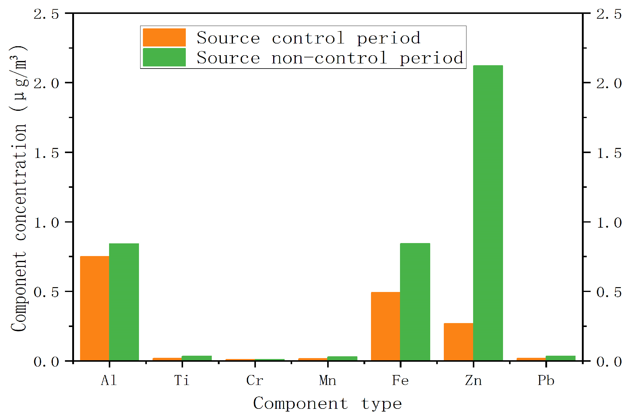
From the data in Table 2, it is observed that when the source control strategy was not implemented, the outdoor PM2.5 concentration was 40.08 μg/m3, but after the source control strategy was implemented, the outdoor PM2.5 concentration was reduced to 26.31 μg/m3, indicating that the source control strategy implemented in Beijing and its surrounding areas during the “Parade Blue” period could effectively reduce the atmospheric fine particle concentration. The same conclusion can be drawn by comparing the concentrations of each component of PM2.5 in Table 3, that is, the concentrations of each component of PM2.5 in the source non-control period were significantly higher than those of each component in the source control period.
The concentration changes in PM2.5 components during the source control period and source non-control period are shown in Figure 3.

3.2. Comparison of EPACMB8.2 and NKCMB1.0 Receptor Models

3.2.1. Source Control Period Comparison Results

The results of source resolution during the source control period by two different receptor model software, EPACMB8.2 and NKCMB1.0, are shown in Table 4.
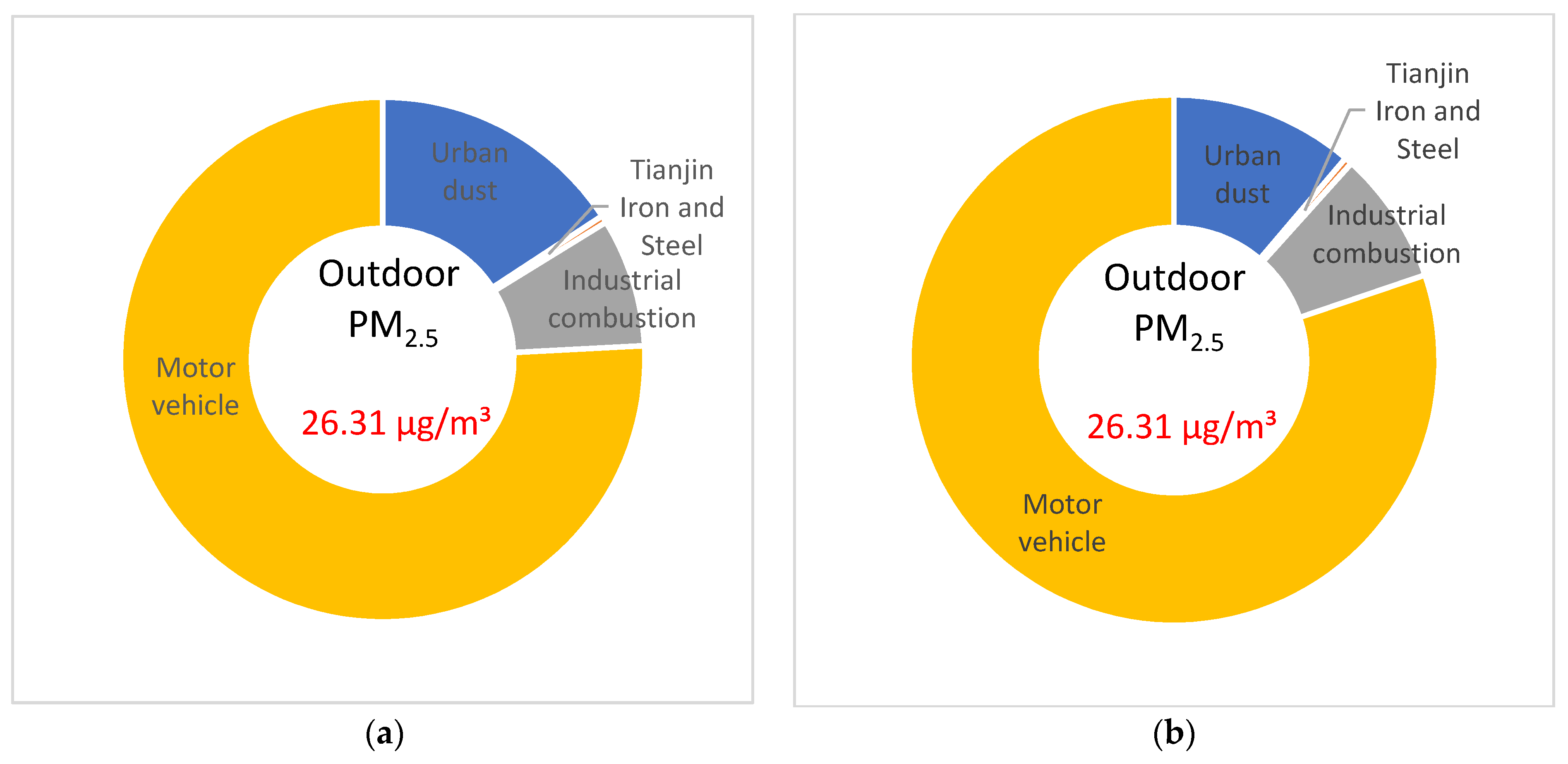
Based on the above data, a pie chart displaying the contribution rates of each emission source class in the source control period was drawn using EPACMB8.2 and NKCMB1.0 receptor model source analysis as shown in Figure 4.
From the above data, it can be observed that the relative error of NKCMB1.0 ranges between −29–6% based on the contribution rate of each emission source obtained by EPACMB8.2 source analysis, and the relative error of all the emission sources ranges between 2–6% except that of urban dust. Motor vehicle emissions are the main pollutant emission source category, with a contribution rate of around 80%, followed by urban dust and industrial combustion, with a contribution rate of around 10%. This may also be because the selected emission sources are similar during source analysis, that is, the components of multiple source classes are similar or proportional, and CMB will be interfered with by the collinearity of emission sources, which will affect the source analysis of the receptor model, and thus make the source contribution rate appear negative.
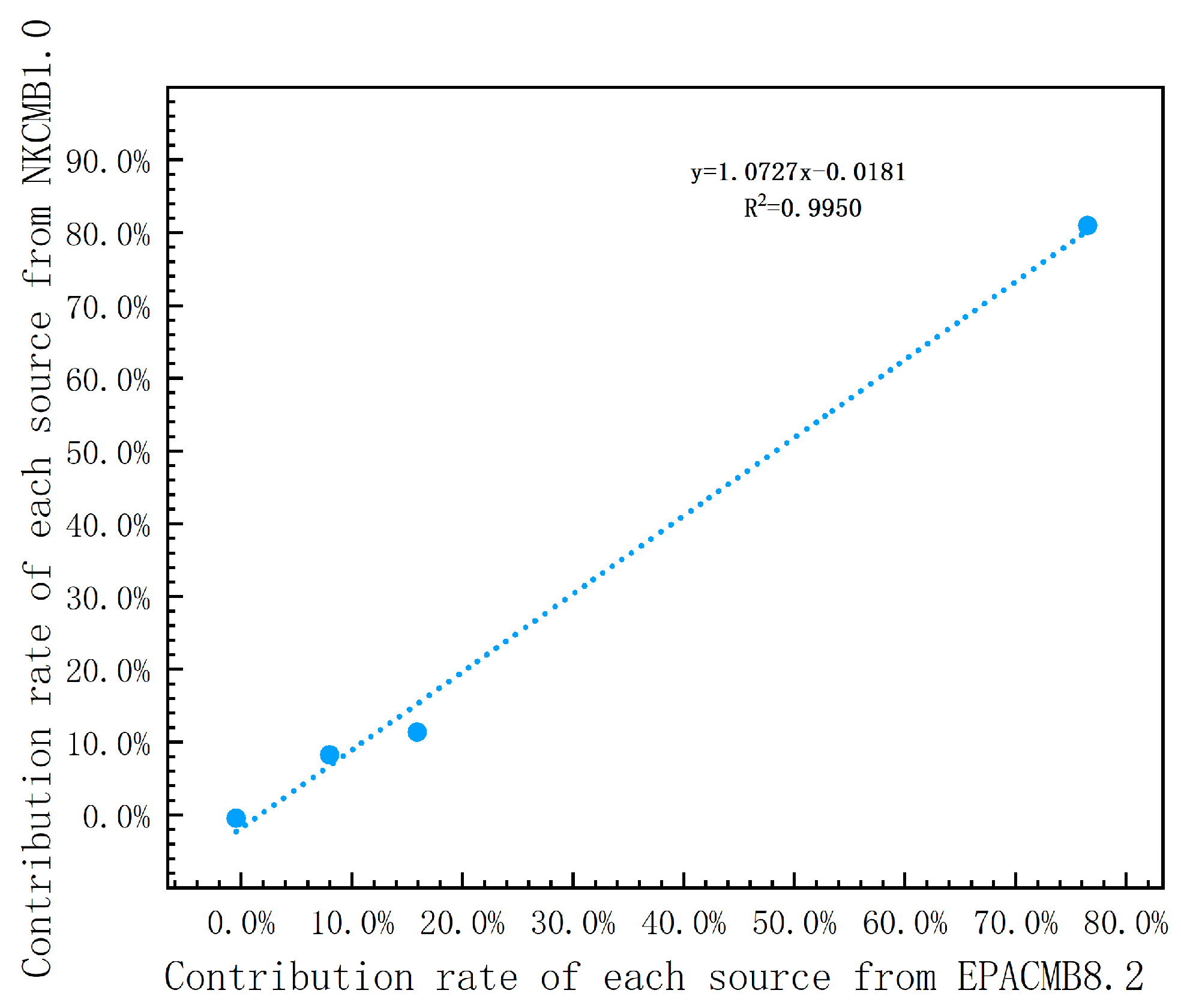
The data obtained from the two receptor models were fitted, and the results are shown in Figure 5.
As can be seen from Figure 5, the results of the linear fitting show a slope of 1.0727, an intercept of −0.0181, and R 2 = 0.995 . The results obtained by using different analysis software of the same receptor model EPACMB8.2 and NKCMB1.0 for source analysis in the source control period basically showed a linear relationship. Using SPSS software to process the two groups of data, the significance level was 0.003. This showed that the conclusions drawn from source analysis were the same, indicating that the calculation results of the contribution rates of the above different pollutant discharge source types were relatively reliable.

3.2.2. Source Non-Control Period Comparison Result

The results of source resolution performed by the EPACMB8.2 and NKCMB1.0 receptor model software in the source non-control periods are shown in Table 5.
Through observing the data in Table 5, pie charts displaying the contribution rates of various emission sources in the source non-control period obtained from source analysis of EPACMB8.2 and NKCMB1.0 receptor model are drawn as shown in Figure 6.
From the above data, it can be observed that the relative error of NKCMB1.0 ranges between −36–8% based on the contribution rate of each emission class obtained by EPACMB8.2 source analysis, and the relative error of all the emission sources ranges between 0–8% except that of urban dust. Compared with the source control period, industrial combustion and motor vehicle emissions in the source non-control period are the main sources of pollutants. The contribution rate of motor vehicle emissions is nearly 60%, and the contribution rate of industrial combustion is more than 40%, while the contribution rate of urban dust is very small, measuring less than 2%. Among them, the contribution rate of Tianjin Iron and Steel is negative, the reason for this result 3.2.1 has been analyzed and will not be repeated here.
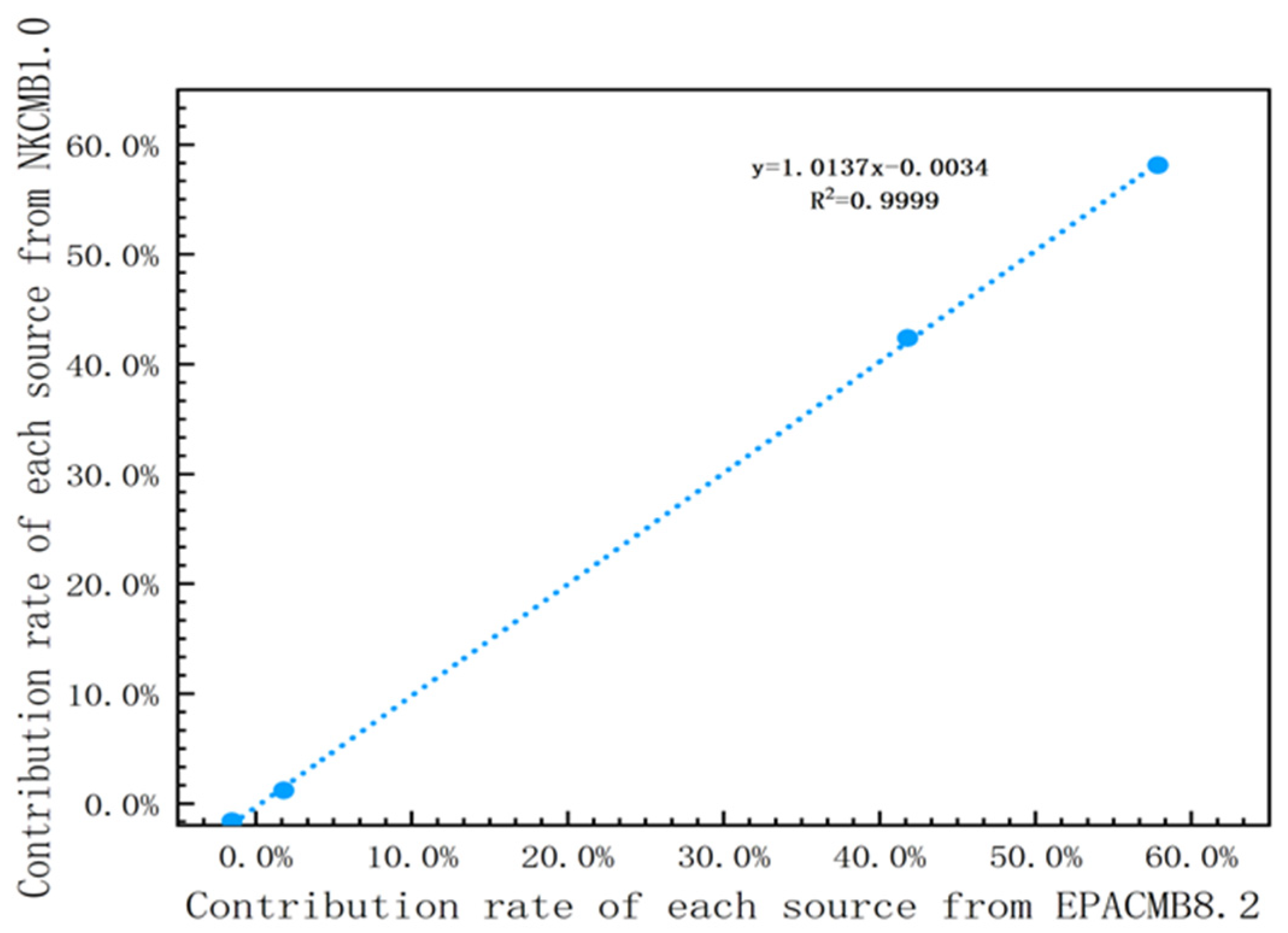
The data obtained from the two receptor models were fitted, and the results are shown in Figure 7.
From Figure 7, the results of the linear fitting show a slope of 1.0137, intercept of −0.0034, and R2 = 0.9999. Moreover, it can be seen that the results of source analysis in the source control period using different analysis software of EPACMB8.2 and NKCMB1.0, two identical receptor models, basically presented a linear relationship. Using SPSS (R27.0.1.0) software to process the two sets of data, the significance level was less than 0.001. This indicated that the conclusions drawn from source analysis were the same, which could also indicate that the calculation results of the contribution rates of the above different pollutant discharge source types were reliable.

3.2.3. Comparison Results and Discussion

The results of source analysis during the source control period were obtained by using different analysis software of EPACMB8.2 and NKCMB1.0, two identical receptor models, as shown in Table 6.
The results of source analysis using EPACMB8.2 and NKCMB1.0, two different analysis software of the same receptor model, show that the contribution rate to pollutants in the source control period and the source non-control period is closely related to the source control strategy. During the implementation of source control measures in Beijing, the contribution of motor vehicle emissions to the three emission sources of urban dust, industrial combustion and motor vehicle emissions is much greater than that of the two emission sources of urban dust and industrial combustion. However, when the implementation of the source control measures is not implemented, the contribution of industrial combustion increases significantly. The contribution of motor vehicle emission and industrial combustion is significantly greater than that of urban dust. In both the source control period and the source non-control period, the largest contribution to pollutants is motor vehicle emission, but the contribution of motor vehicle emission is significantly different from that of industrial combustion emission during the source control period. When the source is not controlled, the contribution rate of industrial combustion increases significantly, while the contribution rate of motor vehicle emission decreases, and these two sources are significantly higher than that of urban dust emission sources. This result indicates that the contribution rate of each emission source is closely related to the emission source control strategy implemented in Beijing. Therefore, in order to improve outdoor air quality and reduce outdoor particulate pollution, attention should be paid to the impact of industrial combustion and vehicle emissions on outdoor air quality.

3.3. Limitations and Prospects

The contribution rate of each emission source class obtained by using two different source analysis software, EPACMB8.2 and NKCMB1.0, will be negative. The reason for the negative value is as follows [38]: (1) There are uncertain source classes in the emission source classes for source analysis. The source class refers to the contribution rate of the source class being less than the limit of detection of the source class, that is, the contribution rate of the source class has a large deviation; (2) There are two or more collinear sources in the emission source class for source analysis, and the components of these emission source classes are similar or proportional. The diagnosis of such errors can be tested by T-statistics (TSTAT) and singular value decomposition (SVD). It was found through the T-statistic (TSAT) method that TSAT < 2 served as a diagnostic tool to determine whether a source class was an uncertain source class. If TSAT fell below 2, the contribution rate of the source class was found to be below the limit of detection, making it an uncertain source. The singular value decomposition rule was another diagnostic method to determine whether some source classes were collinear source classes. It can be seen from the T-statistical results obtained by NKCMB1.0 that the TSAT of sources such as Tianjin Iron and Steel with negative contribution rates is less than 2, making these sources an uncertain source type.
Diagnostic values were obtained in this case as shown in Table 7.
As shown in Table 7, source analysis was conducted using two different receptor model software, EPACMB8.2 and NKCMB1.0. The sum of squares of residuals (χ2) and the regression coefficient (R2) suggest that the fitting results were good; however, the percent mass (PM) diagnosis did not meet expectations, resulting in a larger sum of calculated contributions from each source class relative to the measured total mass concentration of receptors. In the future analysis of PM2.5 source classes, it is necessary to consider the correlation between the selected source classes to improve the diagnosis result.
In future research on “particulate matter pollution”, the relationship between specific source control strategies and emission source categories can be further investigated to develop more constructive and targeted source control strategies.
In future studies, more sampling points can be widely distributed in the study area to obtain more accurate results. Further research on preventing outdoor particulate matter from entering indoor areas and purifying the introduced indoor air can be carried out. At the same time, the indoor fine particle pollution and its source, and indoor air purification should be paid attention to without considering the outdoor fine particle pollution source.

4. Conclusions

In this study, CMB was used to analyze the source of the receptor. The proportions of each outdoor emission source’s contribution to the particulate matter pollution in the source control period and source non-control period were obtained using different analysis software, EPACMB8.2 and NKCMB1.0, from two identical receptor models, and the reliability of the source analysis results was compared. The results indicate that the source control strategy has an impact on the proportion of source contribution. Research shows that the source control strategy has relatively conspicuous effects, which will reduce the outdoor fine particle concentration and bring obvious environmental and health benefits. Relevant departments should actively formulate appropriate source control measures and encourage the public to respond positively, for example, a planned closing down or restrictions of industrial factory activity and low-carbon travel, etc. Compared with previous studies on PM2.5 source contribution rate in Beijing, this study used the objective condition of “Parade Blue” to analyze the change in PM2.5 source contribution rate before and after source control. Compared with previous studies on the change in PM2.5 concentration during the “Parade Blue” period, this study analyzed the change in source contribution rate of PM2.5 before and after the source control period. However, there is an objective factor of uncertainty in the emission source class analyzed by source analysis, and the contribution rate of each emission source class obtained by EPACMB8.2 and NKCMB1.0 source analysis software will all be negative. Therefore, in future PM2.5 source class analysis, attention should be paid to the correlation between the selected source classes. In the future research on “particulate matter pollution”, the relationship between specific source control strategies and emission source types can be further studied, and more constructive and targeted source control strategies can be proposed.

Author Contributions

Conceptualization, Y.X.; methodology, Y.X.; software, A.G.; validation, Y.X., Y.G. and A.G.; formal analysis, Y.G.; investigation, Y.G.; resources, Y.X.; data curation, A.G.; writing—original draft preparation, Y.X. and A.G.; writing—review and editing, Y.G.; visualization, Y.G.; supervision, Y.X.; project administration, Y.X.; funding acquisition, Y.X. All authors have read and agreed to the published version of the manuscript.

Funding

This research was funded by the National Key Research and Development Plan from the Ministry of Science and Technology of China grant No.2022YFC3702604.

Institutional Review Board Statement

Not applicable.

Informed Consent Statement

Not applicable.

Data Availability Statement

The data presented in this study are available on request from the corresponding author. The data are not publicly available due to Ph.D. thesis restrictions.

Conflicts of Interest

The authors declare no conflict of interest.

References

  1. Wei, T.T.; Tang, M. Biological effects of airborne fine particulate matter (PM2.5) exposure on pulmonary immune system. Environ. Toxicol. Pharmacol. 2018, 60, 195–201. [Google Scholar] [CrossRef] [PubMed]
  2. Jin, X.T.; Xue, B.; Zhou, Q.F.; Su, R.J.; Li, Z.Y. Mitochondrial damage mediated by ROS incurs bronchial epithelial cell apoptosis upon ambient PM2.5 exposure. J. Toxicol. Sci. 2018, 43, 101–111. [Google Scholar] [CrossRef] [PubMed]
  3. Gutiérrez-Avila, I.; Rojas-Bracho, L.; Riojas-Rodríguez, H.; Kloog, I.; Just, A.C.; Rothenberg, S.J. Cardiovascular and Cerebrovascular Mortality Associated With Acute Exposure to PM2.5 in Mexico City. Stroke 2018, 49, 1734–1736. [Google Scholar] [CrossRef] [PubMed]
  4. Xing, Y.F.; Xu, Y.H.; Shi, M.H.; Lian, Y.X. The impact of PM2.5 on the human respiratory system. J. Thorac Dis. 2016, 8, E69–E74. [Google Scholar] [CrossRef] [PubMed]
  5. Wu, Y.Y.; Gu, B.J.; Erisman, J.W.; Reis, S.; Fang, Y.Y.; Lu, X.H.; Zhang, X.M. PM2.5 pollution is substantially affected by ammonia emissions in China. Environ. Pollut. 2016, 218, 86–94. [Google Scholar] [CrossRef]
  6. Yang, S.Y.; Fang, D.L.; Chen, B. Human health impact and economic effect for PM2.5 exposure in typical cities. Appl. Energy 2019, 249, 316–325. [Google Scholar] [CrossRef]
  7. Kuncoro, C.B.D.; Adristi, C.; Asyikin, M.B.Z. Smart Wireless Particulate Matter Sensor Node for IoT-Based Strategic Monitoring Tool of Indoor COVID-19 Infection Risk via Airborne Transmission. Sustainability 2022, 14, 14433. [Google Scholar] [CrossRef]
  8. Ruinong, L. Column: Air Quality Assurance for Commemorating the 70th Anniversary of the Victory of the Chinese People’s War of Resistance against Japanese Aggression and the World Anti-Fascist War; Ministry of Foreign Affairs: Beijing, China, 2016.
  9. Yin, L.R.; Wang, L.; Huang, W.Z.; Liu, S.; Yang, B.; Zheng, W.F. Spatiotemporal Analysis of Haze in Beijing Based on the Multi-Convolution Model. Atmosphere 2021, 12, 1408. [Google Scholar] [CrossRef]
  10. Liu, Y.; Tian, J.W.; Zheng, W.F.; Yin, L.R. Spatial and temporal distribution characteristics of haze and pollution particles in China based on spatial statistics. Urban Clim. 2022, 41, 101031. [Google Scholar] [CrossRef]
  11. Chen, J.; Liu, Z.X.; Yin, Z.T.; Liu, X.; Li, X.L.; Yin, L.R.; Zheng, W.F. Predict the effect of meteorological factors on haze using BP neural network. Urban Clim. 2023, 51, 101630. [Google Scholar] [CrossRef]
  12. Yin, L.R.; Wang, L.; Huang, W.Z.; Tian, J.W.; Liu, S.; Yang, B.; Zheng, W.F. Haze Grading Using the Convolutional Neural Networks. Atmosphere 2022, 13, 522. [Google Scholar] [CrossRef]
  13. Xu, L.; Zhang, J.; Sun, X.; Xu, S.C.; Shan, M.; Yuan, Q.; Liu, L.; Du, Z.H.; Liu, D.T.; Xu, D.; et al. Variation in Concentration and Sources of Black Carbon in a Megacity of China During the COVID-19 Pandemic. Geophys. Res. Lett. 2020, 47, e2020GL090444. [Google Scholar] [CrossRef] [PubMed]
  14. Xu, W.; Song, W.; Zhang, Y.Y.; Liu, X.J.; Zhang, L.; Zhao, Y.H.; Liu, D.Y.; Tang, A.H.; Yang, D.W.; Wang, D.D.; et al. Air quality improvement in a megacity: Implications from 2015 Beijing Parade Blue pollution control actions. Atmos. Chem. Phys. 2017, 17, 31–46. [Google Scholar] [CrossRef]
  15. Yang, S.J.; Zhang, Y.; Shang, J.; Li, Z.Q.; de Foy, B.; Schauer, J.J.; Zhang, Y.X. “Military Parade Blue Skies” in Beijing: Decisive Influence of Meteorological Factors on Transport Channel and Atmospheric Pollutant Concentration Level. Atmosphere 2021, 12, 636. [Google Scholar] [CrossRef]
  16. Xue, Y.F.; Wang, Y.; Li, X.F.; Tian, H.Z.; Nie, L.; Wu, X.Q.; Zhou, J.R.; Zhou, Z. Multi-dimension apportionment of clean air “parade blue” phenomenon in Beijing. J. Environ. Sci. 2018, 65, 29–42. [Google Scholar] [CrossRef] [PubMed]
  17. Yang, X.W.; Cheng, S.Y.; Li, J.B.; Lang, J.L.; Wang, G. Characterization of Chemical Composition in PM2.5 in Beijing before, during, and after a Large-Scale International Event. Aerosol Air Qual. Res. 2017, 17, 896–907. [Google Scholar] [CrossRef]
  18. Xue, Y.F.; Zhang, S.H.; Nie, T.; Cao, X.Z.; Shi, A.J. Environmental Effective Assessment of Control Measures Implemented by Clean Air Action Plan (2013-2017) in Beijing, China. Atmosphere 2020, 11, 189. [Google Scholar] [CrossRef]
  19. Chen, M.; Wang, P.F.; Chen, Q.; Wu, J.D.; Chen, X.Y. A clustering algorithm for sample data based on environmental pollution characteristics. Atmos. Environ. 2015, 107, 194–203. [Google Scholar] [CrossRef]
  20. Faridi, S.; Yousefian, F.; Roostaei, V.; Harrison, R.M.; Azimi, F.; Niazi, S.; Naddafi, K.; Momeniha, F.; Malkawi, M.; Safi, H.A.M.; et al. Source apportionment, identification and characterization, and emission inventory of ambient particulate matter in 22 Eastern Mediterranean Region countries: A systematic review and recommendations for good practice. Environ. Pollut. 2022, 310, 119889. [Google Scholar] [CrossRef]
  21. Feng, X.X.; Feng, Y.L.; Chen, Y.J.; Cai, J.J.; Li, Q.; Chen, J.M. Source apportionment of PM2.5 during haze episodes in Shanghai by the PMF model with PAHs. J. Clean. Prod. 2022, 330, 129850. [Google Scholar] [CrossRef]
  22. Xu, X.M.; Zhang, H.F.; Chen, J.M.; Li, Q.; Wang, X.F.; Wang, W.X.; Zhang, Q.Z.; Xue, L.K.; Ding, A.J.; Mellouki, A. Six sources mainly contributing to the haze episodes and health risk assessment of PM2.5 at Beijing suburb in winter 2016. Ecotoxicol. Environ. Saf. 2018, 166, 146–156. [Google Scholar] [CrossRef] [PubMed]
  23. Jain, S.; Sharma, S.K.; Vijayan, N.; Mandal, T.K. Seasonal characteristics of aerosols (PM2.5 and PM10) and their source apportionment using PMF: A four year study over Delhi, India. Environ. Pollut. 2020, 262, 114337. [Google Scholar] [CrossRef] [PubMed]
  24. Jiang, N.; Wang, K.; Yu, X.; Su, F.C.; Yin, S.S.; Li, Q.; Zhang, R.Q. Chemical Characteristics and Source Apportionment by Two Receptor Models of Size-segregated Aerosols in an Emerging Megacity in China. Aerosol Air Qual. Res. 2018, 18, 1375–1390. [Google Scholar] [CrossRef]
  25. Moreno, T.; Kojima, T.; Amato, F.; Lucarelli, F.; de la Rosa, J.; Calzolai, G.; Nava, S.; Chiari, M.; Alastuey, A.; Querol, X.; et al. Daily and hourly chemical impact of springtime transboundary aerosols on Japanese air quality. Atmos. Chem. Phys. 2013, 13, 1411–1424. [Google Scholar] [CrossRef]
  26. Nojgaard, J.K.; Peker, L.; Pernov, J.B.; Johnson, M.S.; Bossi, R.; Massling, A.; Lange, R.; Nielsen, I.E.; Prevot, A.S.H.; Eriksson, A.C.; et al. A local marine source of atmospheric particles in the High Arctic. Atmos. Environ. 2022, 285, 119241. [Google Scholar] [CrossRef]
  27. Ma, L.; Dadashazar, H.; Braun, R.A.; MacDonald, A.B.; Aghdam, M.A.; Maudlin, L.C.; Sorooshian, A. Size-resolved characteristics of water-soluble particulate elements in a coastal area: Source identification, influence of wildfires, and diurnal variability. Atmos. Environ. 2019, 206, 72–84. [Google Scholar] [CrossRef]
  28. Roy, D.; Singh, G.; Yadav, P. Identification and elucidation of anthropogenic source contribution in PM10 pollutant: Insight gain from dispersion and receptor models. J. Environ. Sci. 2016, 48, 69–78. [Google Scholar] [CrossRef]
  29. Tseng, Y.L.; Yuan, C.S.; Wong, K.W.; Lin, C. Chemical fingerprints and source resolution of atmospheric fine particles in an industrial harbor based on one-year intermittent field sampling data. Sci. Total Environ. 2023, 868, 161335. [Google Scholar] [CrossRef]
  30. Allen, D. Attributing Atmospheric Methane to Anthropogenic Emission Sources. Acc. Chem. Res. 2016, 49, 1344–1350. [Google Scholar] [CrossRef]
  31. Yin, J.; Cumberland, S.A.; Harrison, R.M.; Allan, J.; Young, D.E.; Williams, P.I.; Coe, H. Receptor modelling of fine particles in southern England using CMB including comparison with AMS-PMF factors. Atmos. Chem. Phys. 2015, 15, 2139–2158. [Google Scholar] [CrossRef]
  32. EPA. Chemical Mass Balance (CMB) Model. Available online: https://www.epa.gov/scram/chemical-mass-balance-cmb-model (accessed on 10 June 2023).
  33. The State Environment Protection Key Laboratory of Urban Particulate Air Pollution Protection. NKCMB1.0. Available online: https://env.nankai.edu.cn/air/ (accessed on 25 June 2023).
  34. Friedlander, S.K. Chemical element balances and identification of air pollution sources. Environ. Sci. Technol. 1973, 7, 235–240. [Google Scholar] [CrossRef] [PubMed]
  35. Watson, J.G. Chemical Element Balance Receptor Model Methodology for Assessing the Sources of Fine and Total Suspended Particulate Matter in Portland, Oregon; Oregon Graduate Institute of Science and Technology: Portland, OR, USA, 1979. [Google Scholar]
  36. Thomas, C.C. EPA-CMB8.2Users Manual [EB/OL]. Available online: https://www.epa.gov/sites/production/files/2020-10/documents/epa-cmb82manual.pdf (accessed on 29 July 2023).
  37. Wang, T.; Hua, Y.; Xu, Q.-C.; Wang, S.-X. Source Apportionment of PM2.5 in Suburban Area of Beijing-Tianjin-Hebei Region in Autumn and Winter. Huan Jing Ke Xue = Huanjing Kexue 2019, 40, 1035–1042. [Google Scholar] [CrossRef] [PubMed]
  38. Zhu, T.; Feng, Y.C. Source Analysis of Atmospheric Particulate Matter: Principle, Technology and Application; Science Press: Beijing, China, 2012. [Google Scholar]
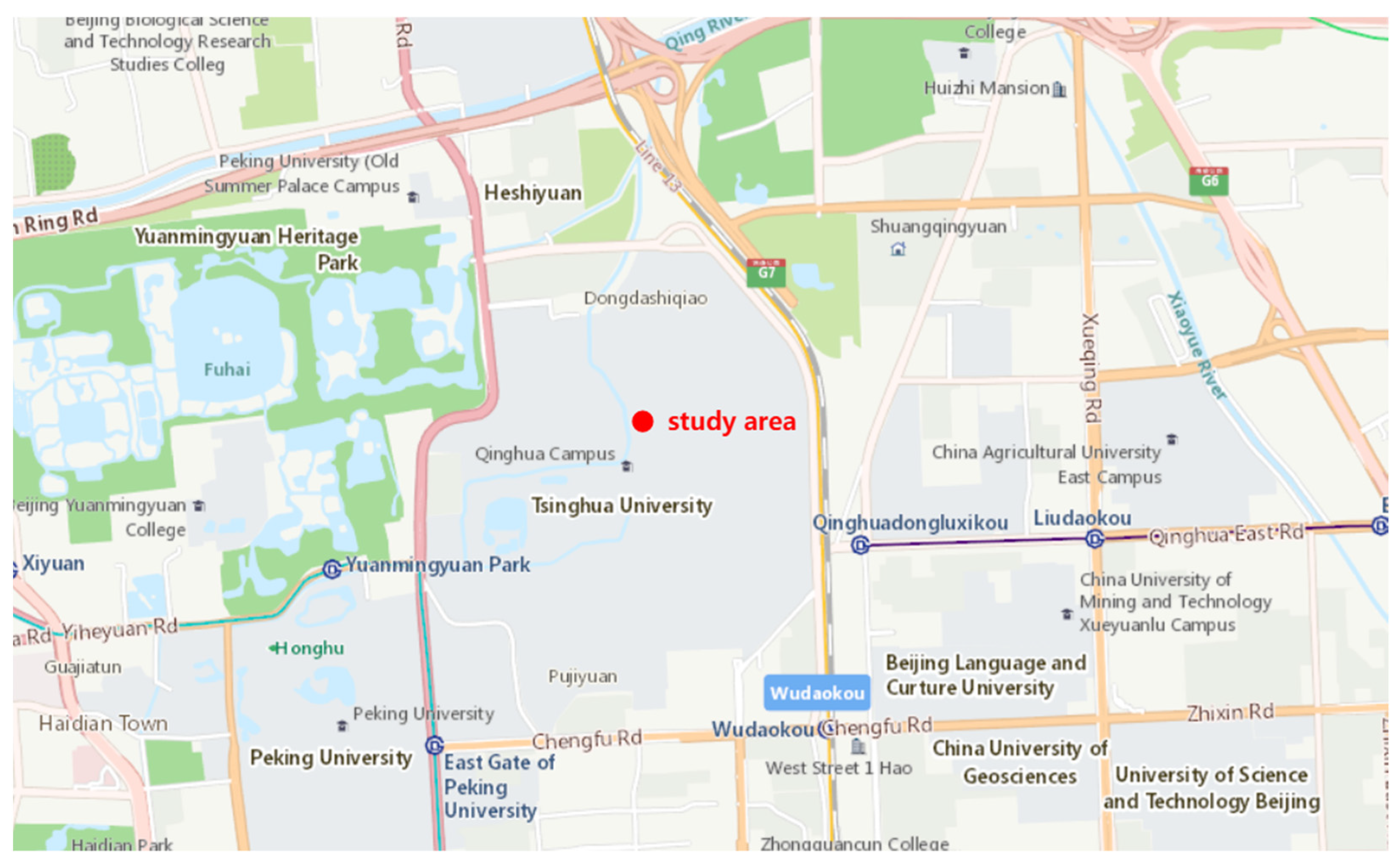
Figure 1. Specific location of the study area.
Atmosphere 14 01639 g001
Figure 2. Flow Diagram of CMB Source Apportionment.
Atmosphere 14 01639 g002
Figure 3. Concentration of each component in source control period and source (non-control) period.
Atmosphere 14 01639 g003
Figure 4. (a) Contribution rates of each emission source obtained by EPACMB8.2 during the control period, and (b) contribution rates of each emission source obtained by NKCMB1.0 during the control period.
Atmosphere 14 01639 g004
Figure 5. Fitting of the contribution rates of each emission source from EPACMB8.2 and NKCMB1.0 during the source control period.
Atmosphere 14 01639 g005
Figure 6. (a) Contribution rates of each emission source obtained by EPACMB8.2 during the non-control period, and (b) contribution rates of each emission source obtained by NKCMB1.0 during the non-control period.
Atmosphere 14 01639 g006
Figure 7. Fitting of the contribution rates of each emission source obtained from EPACMB8.2 and NKCMB1.0 in the source non-control period.
Atmosphere 14 01639 g007
Table 1. Measured concentration of each component from each emission source (μg/m3).
Emission SourceAlTiCrMnFeZnPb
Urban dust0.05470.005500.00030.02660.00050
Tianjin Iron and Steel0.02810.00470.00100.00980.23460.01830.0182
Industrial combustion0.00380.00030.00040.00040.01420.01690.0001
Gasoline car0.00240.00020.00020.00010.00400.00270.0005
Diesel car0.00240.00130.00100.00080.00540.00080
Table 2. Concentration values of receptor components in source control period and source non-control period (μg/m3).
PeriodDatePM2.5AlTiCrMnFeZnPb
Source
control
21 August 2015–4 September 201526.310.7500.0190.0100.0170.4930.2690.020
Non-source
control
17 August 2015–20 August 2015
5 September 2015–7 September 2015
40.080.8420.0330.0110.0300.8442.1220.035
Table 3. Measured concentration of PM2.5 components on different filtration membranes (μg/m3).
PeriodDateNumberAlTiCrMnFeZnPb
Non-source
control
17 August 2015T212.28860.08260.01740.05611.56970.39920.0545
19 August 2015T040.86360.03330.01060.02730.71210.31360.0311
19 August 2015T220.75970.02990.00830.02290.63750.25760.0201
Source control21 August 2015T231.06060.03480.01210.02730.80450.26740.0159
22 August 2015T030.75150.04020.01210.03110.95230.30230.0591
23 August 2015T190.45550.01730.01100.01550.53300.30210.0110
24 August 2015T254.63990.01900.00910.01900.64410.25510.0099
25 August 2015T110.48930.01930.01080.01310.45380.24740.0085
26 August 2015T100.41730.01600.01070.01220.38760.25560.0076
27 August 2015T180.39000.01800.01200.01430.38480.25350.0135
28 August 2015T240.72600.02760.01030.02530.67870.29040.0229
29 August 2015T070.35070.02260.00780.01870.50060.26940.0320
30 August 2015T120.22570.01300.01150.01220.30530.26090.0191
31 August 2015T170.12030.00550.00860.00550.14760.24130.0062
1 September 2015T050.20950.00890.01050.00810.25790.24340.0097
2 September 2015T080.30780.01030.00870.00790.28330.25960.0071
3 September 2015T130.35590.01970.00870.03390.56500.31490.0537
4 September 2015T090.16470.00930.00770.00770.18320.23500.0186
Non-source
control
5 September 2015T200.49010.01780.00850.02710.902112.9360.0433
6 September 2015T160.66620.03130.01070.03051.05650.33350.0247
7 September 2015T150.65790.02550.01080.03560.84340.37650.0495
Table 4. Contribution rates of different emission sources in EPACMB8.2 and NKCMB1.0 source control periods.
Emission SourceEPACMB8.2NKCMB1.0
Urban dust15.92%11.32%
Tianjin Iron and Steel−0.45%−0.46%
Industrial combustion8.01%8.20%
Motor vehicle76.52%80.95%
Table 5. Contribution rates of different emission sources in EPACMB8.2 and NKCMB1.0 source non-control periods.
Emission SourceEPACMB8.2NKCMB1.0
Urban dust1.81%1.16%
Tianjin Iron and Steel−1.50%−1.62%
Industrial
combustion
41.82%42.36%
Motor vehicle57.86%58.11%
Table 6. Contribution rate of outdoor emission sources in source control period and source non-control period.
Emission SourceSource Control EPACMB8.2Source Control NKCMB1.0Non-Source Control EPACMB8.2Non-Source Control NKCMB1.0
Urban dust15.92%11.32%1.81%1.16%
Tianjin Iron and Steel−0.45%−0.46%−1.50%−1.62%
Industrial combustion8.01%8.20%41.82%42.36%
Motor vehicle76.52%80.95%57.86%58.11%
Table 7. Diagnostic results of EPACMB8.2 and NKCMB1.0 data.
PeriodReceptor Model Softwaredf
(Degrees of Freedom)
PM (%)χ2R2
Source
control
EPACMB8.22265.50.061.00
NKCMB1.02196.90.060.99
Non-source
control
EPACMB8.22542.90.070.99
NKCMB1.02215.70.080.99
Disclaimer/Publisher’s Note: The statements, opinions and data contained in all publications are solely those of the individual author(s) and contributor(s) and not of MDPI and/or the editor(s). MDPI and/or the editor(s) disclaim responsibility for any injury to people or property resulting from any ideas, methods, instructions or products referred to in the content.