Multiwave Matrix Polarization Lidar

Abstract

Remote control of the state of the atmosphere is an urgent problem nowadays. The problem of remote monitoring of the optical parameters of the atmosphere is solved using a matrix polarization lidar (MPL). The scattering matrix obtained from polarization measurements contains complete information on the scattering parameters in the atmosphere. The purpose of the present research is the derivation of the theory and description of methods for solving problems of practical implementation of the multiwave MPL (MMPL). The problem is considered within the framework of the concept of the unified methodological approach to polarization studies. The MMPL operation principle is based on simultaneous use for sensing of the first, second, and third harmonics of radiation of a widespread Nd:YAG laser. The basis for achieving this purpose is provided by new methods of optical selection of the polarization components of radiation received in the experiment, methods of conducting polarization studies, and new solutions in experimental data processing methods. It has been shown that this challenge can be solved within the framework of simple solutions. Thus, the proposed MMPL is structurally simple and compact and can be implemented in mobile polarization lidar systems.

1. Introduction

A significant amount of gaseous and aerosol impurities is always present in the atmospheric air. In addition to H₂O in different phase states, a huge number of solid and liquid particles are constantly added to the earth’s atmosphere as a result of natural processes such as dust storms, volcano eruptions, forest fires, soil erosion, etc. [1,2,3].

As shown in presentation [4] at the 29th International Conference on 26–30 June 2023, Moscow, the occurrence of new optical materials and progress in their processing methods opens up the possibility of further development of polarization sensing. In this work, we consider the theory and problems of practical implementation of the multiwave matrix polarization lidar (MMPL).

Industrial plants, enterprises for the extraction and processing of mineral resources, coal cuts, cars, and airplanes are the main sources of anthropogenic aerosol pollution of the atmosphere. Aerosols are carried away with air masses, rising with them in the upper atmosphere, and are transported at long distances. They significantly affect the properties of the atmosphere, introducing uncertainties in climate change estimates. The smallest aerosol particles—the water vapor condensation nuclei—actively participate in cloud formation. As seen from the foregoing, remote monitoring of atmospheric aerosol characteristics, including particle concentrations, sizes, and shapes, is an urgent problem now. The change in the polarization state of radiation interacting with the aerosol particles depends on their optical and microphysical characteristics and can serve as an indicator of processes occurring in the atmosphere. The problem of remote monitoring of the optical parameters of the atmosphere is solved using a matrix polarization lidar (MPL) by determining the vertical profile of the backscatter matrix in the atmosphere [5,6,7,8,9,10,11,12,13,14,15,16,17,18,19,20,21].

Regular measurements of the backscatter matrices of high-level crystal clouds have started using the “Stratosphere-1M” MPL since the second half of 1988 in the V.E. Zuev Institute of Atmospheric Optics SB RAS. Since then, studies of high-level crystal clouds have been initiated. With the improvement of measurement techniques and accumulation and comprehension of experimental results, it became clear that a unified methodical approach embodied as a paradigm is required to set up and to carry out the polarization experiments as well as to process their results. Following this approach, the results of previous polarization experiments were successfully compared and verified in work [11], and a new qualitative level of scientific knowledge was reached. Having begun, this process gradually develops, being exposed to careful checks on each step. Note that in the description of the proposed MMPL, we follow exactly this paradigm in the light of new results.

The purpose of the present research is the derivation of the theory and description of methods for solving problems of practical implementation of the multiwave MPL (MMPL).

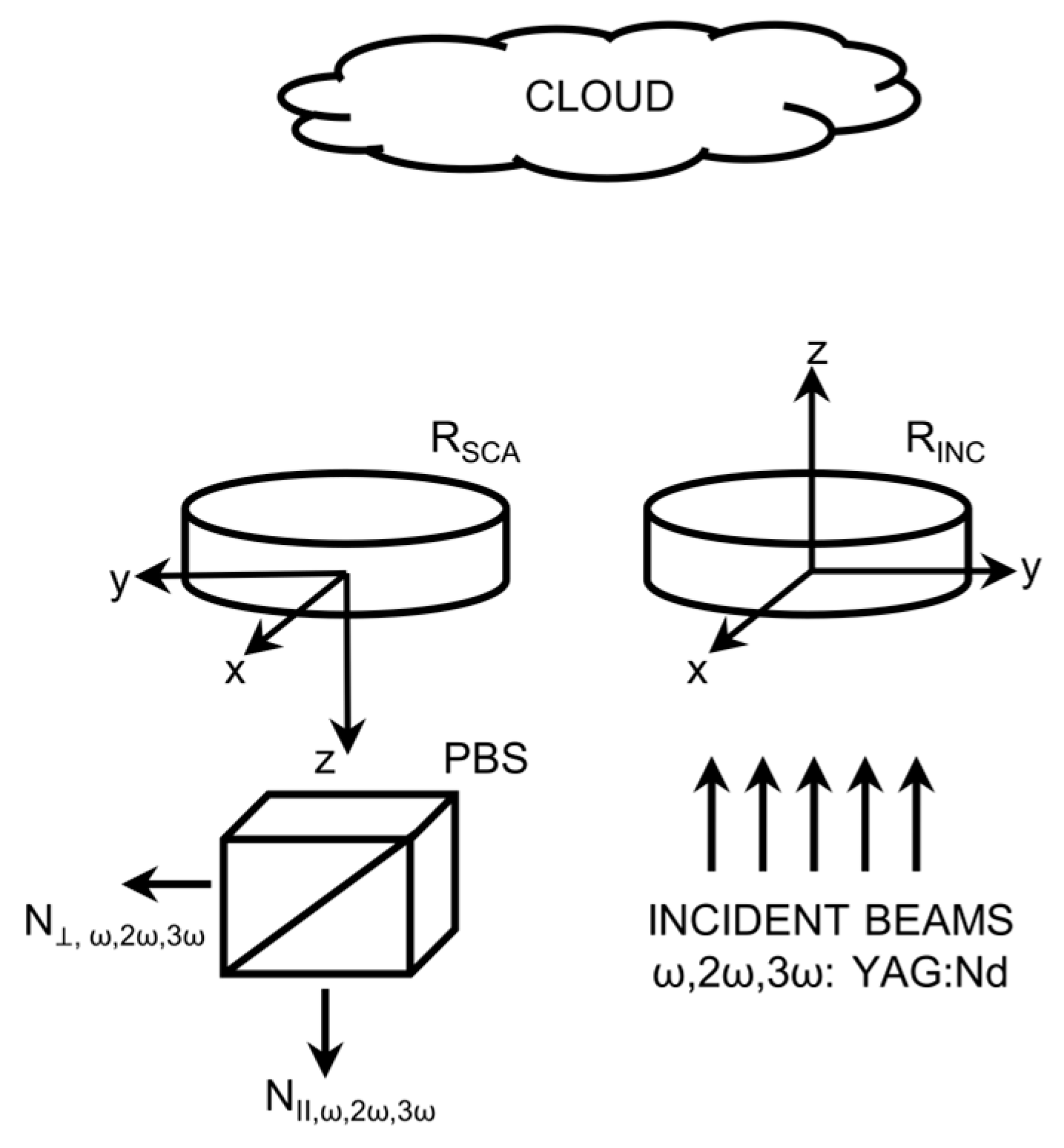
The principle of MMPL operation is based on the simultaneous use of the first, second, and third harmonics of Nd:YAG solid-state laser radiation—the principal laser lines at 355, 532, and 1064 nm. As a result, the vertical profiles of the total backscatter matrix along the sensing path are reconstructed at sensing wavelengths. The dependence of light scattering on particles on the radiation wavelength allows determining the size distribution and morphological structure of various impurities in the atmosphere.

It has been shown that this challenge can be solved within the framework of simple solutions.

In Section 2, the problem of multifrequency polarization sensing is formulated. In terms of the instrumental vectors optimized for this purpose, the system of lidar equations is obtained. Then the procedure of obtaining the so-called scattering matrix equation is presented.

Section 3, Section 3.1, Section 3.2, Section 3.3 and Section 3.4 successively present materials and methods of practical implementation of the MMPL.

In Section 3, we present the MMPL diagram for practical implementation. The MMPL operation principle is based on successive measurements of lidar signals backscattered from the atmosphere.

In Section 3.1, we present the optical selection unit of the MMPL. Variants of practical implementation of the spectral selection unit are given.

In Section 3.2, we consider the method of optical selection of the polarization components. It is shown that the use of the standard calcite crystal Wollaston prism simultaneously solves the problems of selection of the cross-polarized signal components and their wavelength selection. The optical separation method is simple in implementation and eliminates the need for a large number of additional optical elements in the multiwave polarization lidar design.

In Section 3.3, we describe the methodology of the MMPL experiment. The method of polarization measurements has changed significantly. The purpose of the changes consists in increasing the lidar mobility and the efficiency of the method of polarization measurements. The efficiency here is understood as the improvement of such parameters as, for example, acceleration of the measurement procedure at the expense of using only two identical wave plates.

In Section 3.4, we consider in ample detail the methods of processing the measurement results. The method of solving the scattering matrix equation is then described and aimed at estimating values of the backscatter matrix elements in multiwave sensing.

Section 4 gives the results and discussion. Section 5 is devoted to conclusions. Appendix A describes the procedure of obtaining the output instrumental vectors. In Appendix B, the procedure of estimating the backscatter matrix elements based on the GLS method is presented.

2. Theory of MMPL

Here, to derive the system of lidar equations of multiwave polarization sensing as a whole, we use previously accepted designations [16,21,22]. For simplicity, we consider a one-point (collocated) sensing scheme in which we can neglect the spatial separation of the lidar receiver and transmitter.

The simplified optical block diagram of the MMPL is shown in Figure 1.

We consider that scattering particles are within the volume $\Delta V$ at the sensing altitude $h$. The radiation incident on the scattering volume is described by the Stokes vector $S_0={\left(I,Q,U,V\right)}^T$. Designating the Stokes vector of scattered radiation at the receiving point by $S$, we provide the general equation that relates the backscatter matrix to the Stokes vectors [11].

$$S=\left(\Delta V/h^2\right)M_{\pi }\left(\lambda \right)S_0,$$

(1)

where the backscatter matrix elements $M_{\pi }\left(\lambda \right)\equiv M_{\pi }$, in $m^{-1}s{r}^{-1}$, are the volume backscattering coefficients at the wavelength $\lambda$, and $T$ is the transposition index. This is the first-order approximation of multiple scattering theory. The matrix $M_{\pi }$ has the following form:

$$\left(\begin{array}{cccc}{M}_{11}& M_{12}& M_{13}& M_{14}\\ M_{12}& M_{22}& M_{23}& M_{24}\\ -M_{13}& -M_{23}& M_{33}& M_{34}\\ M_{14}& M_{24}& -M_{34}& M_{44}\end{array}\right).$$

(2)

For backscattering, the relationship

$$M_{11}+M_{33}=M_{22}+M_{44}$$

(3)

is also satisfied. The matrix $M_{\pi }$ normalized by the element $M_{11}$ has the form $m_{\pi }=M_{\pi }/M_{11}$.

As a rule, the output radiation at wavelengths of 355, 532, and 1064 nm is linearly polarized. Assume that the reference radiation (for example, at a wavelength of 532 nm) is linearly polarized in the yoz scattering plane, and the irradiance $I$ is normalized by unity. Then, the normalized Stokes vector of laser radiation is

$$s_0\left(\gamma \left(\lambda \right)\right)\equiv s_0={\left(1,\cos 2\gamma ,\sin 2\gamma ,0\right)}^T,$$

(4)

where $\gamma \left(\lambda \right)\equiv \gamma$ is the angle of the polarization plane of radiation at the wavelength $\lambda$ counted from the scattering plane at the reference wavelength. Note that at the reference wavelength, $s_0={\left(1,1,0,0\right)}^T$.

Figure 1 shows the mutual arrangement of the coordinate systems of the MMPL transmitter and receiver at the reference wavelength. The transmitter wave plate $R_{INC}$ is at the angle ${\phi }_{INC}$ in the xoy plane of the coordinate system. The receiver plate $R_{SCA}$ is at the angle ${\phi }_{SCA}$. Scattered radiation passes through the Wollaston prism, and the cross-polarized components are received as signals $N_{II}\equiv N_{II}\left(\lambda \right)$ and $N_{\perp }\equiv N_{\perp }\left(\lambda \right)$ at the corresponding sensing wavelengths (the spectral selection method is considered in Section 3). Thus, the similarity with the scheme of single frequency polarization sensing [21] is preserved.

Some elements of the procedure of carrying out the polarization experiment and MMPL calibration have already been described by us previously. Here we mainly use the general approach proposed for solving the inverse problem of MPL calibration to solve the linear problem of estimating the backscattering matrix elements. Thus, within the framework of the general approach, we demonstrate the principal difference of the methods.

In the successive method of polarization measurements, the transmitter wave plate $R_{INC}$ and the receiver wave plate $R_{SCA}$ are successively set in m angular positions $\left\{ {\phi }_{INC}, {\phi }_{SCA}\right\}$. Accordingly, the backscatter components $\left\{N_{II},N_{\perp }\right\}$ are determined for each sensing wavelength. Assume that these components are recorded from the scattering volume in the altitude range $\Delta h$ located at the distance $h$. For each measurement at the corresponding wavelength, we can write the system of lidar equations in terms of the instrumental vectors. For measurements in the photon counting mode, we obtain [11,16,21]:

$$N_{II}=N{I}_{SCA}^{II}{m}_{\pi }{I}_{INC},$$

(5)

$$N_{\perp }=\kappa N{I}_{SCA}^{\perp }{m}_{\pi }{I}_{INC}.$$

(6)

Here, $\kappa \equiv \kappa \left(\lambda \right)$ is the discrepancy in the optical transmission of the cross-polarized components:

$$N\equiv N\left(\lambda \right)=\eta \left(\lambda \right)N_0\left(\lambda \right)\Delta hA{h}^{-2}{M}_{11}\left(\lambda \right)T^2\left(h,\lambda \right),$$

(7)

$\eta \left(\lambda \right)$ is the loss factor; $N_0\left(\lambda \right)$ is the number of photons per laser pulse; $A$ is the effective receiver aperture; $T^2\left(h,\lambda \right)$ is the atmospheric transmittance at the wavelength $\lambda$; $I_{SCA}^{II}=g_0{M}_{II}{M}_{SCA}$ and $I_{SCA}^{\perp }=g_0{M}_{\perp }{M}_{SCA}$ are the instrumental vectors of the receiver row; $I_{INC}=M_{INC}{s}_0\left({\phi }_{\lambda }\right)$ is the instrumental vector of the transmitter column; $g_0=\left(1, 0, 0, 0\right)$ is the unit row vector; $M_{II/\perp }$ are the Wollaston prism Müller matrices [22]; and $M_{SCA/INC}$ are the Müller matrices of the receiver and transmitter wave plates given by Equation (A5).

It should be noted that the accuracy of the obtained equations is determined by measurement statistics.

As shown in previous work [16,21], if the polarization ratio is written in the form:

$$c\equiv c\left(\lambda \right)=\frac{N_{II}-\alpha N_{\perp }}{N_{II}+\alpha N_{\perp }},$$

(8)

where $\alpha =1/\kappa$, then after substitution of Equations (5) and (6), the polarization equation for the backscatter matrix (for simplicity, the equation for the scattering matrix below) of the ith measurement from the series of $m$ measurements at the wavelength $\lambda$ can be written as follows:

$$I_{SCA}{m}_{\pi }{I}_{INC}=0.$$

(9)

Here, following the terminology of previous work [16,21], the transmitter, $I_{INC}$, and receiver, $I_{SCA}$, modified instrumental vectors are given by Equations (A1)–(A5).

3. MMPL Diagram for Practical Implementation

The purpose of this representation is to present the optimum MMPL configuration that can provide the basis for the development of a wide range of devices. Depending on the aim of the research, they can be mobile or stationary devices.

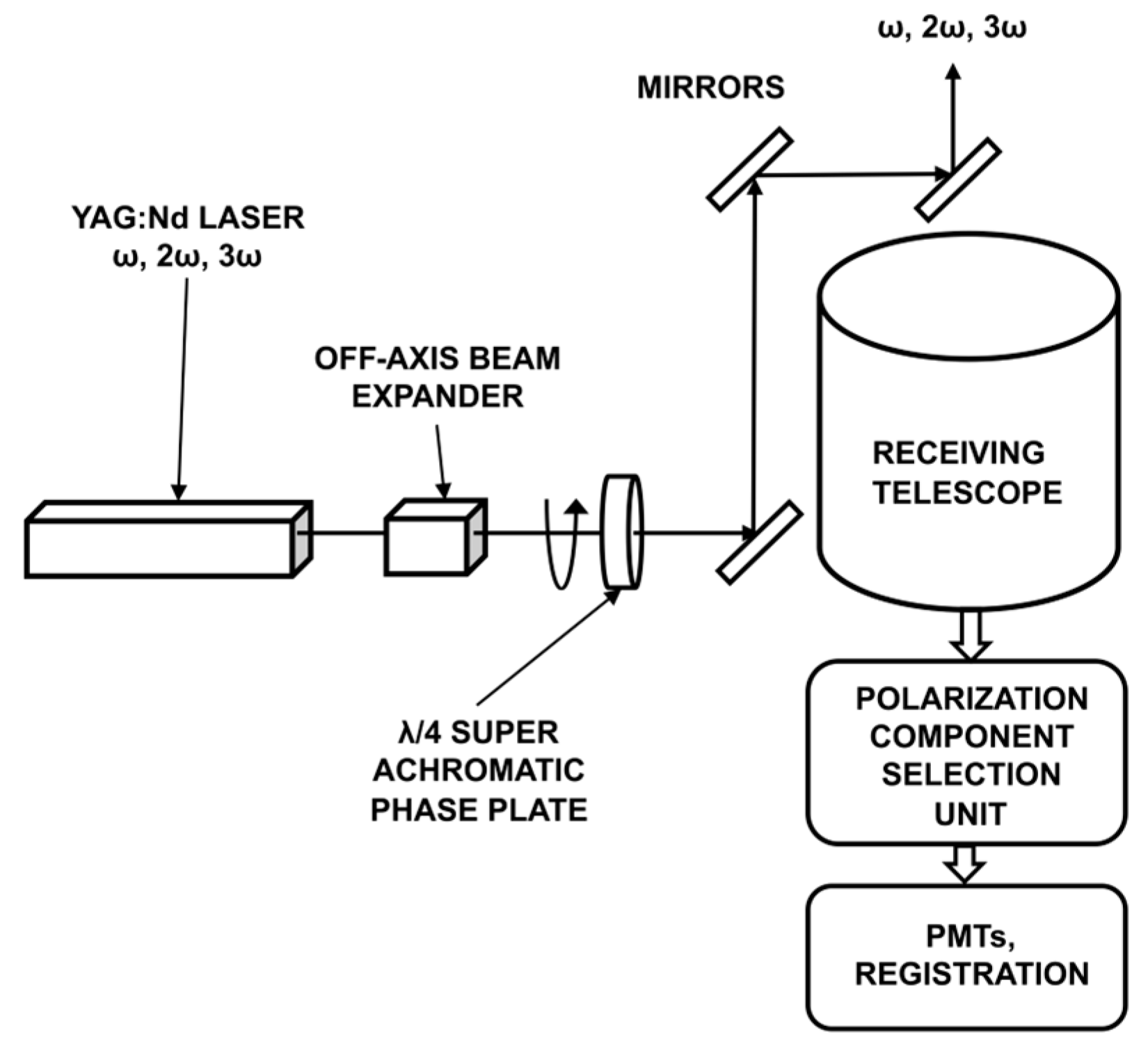
Figure 2 shows the optical block diagram of the MMPL transmitter and receiver units.

Here, Figure 2 schematically shows the main components of the MMPL transmitter and receiver. In the transmitter, Nd:YAG-laser radiation at wavelengths of 355, 532, and 1064 nm passes through the off-axis beam expander and is incident on the quarter-wave phase plate.

The off-axis beam expander is the element of the design of the majority of multiwave lidars. The advantages and disadvantages of these systems are well understood. The super-achromatic wave plate is a fairly new optical element. The robustness of the plate parameters in the wide bandwidth is provided by the optical properties of quartz and magnesium fluoride (MgF2) [23]. The phase plate is achromatic in the wide spectral range of 310–1100 nm. In this range, the plate retardance is within the limits ±0.05 λ of that of the quarter wave plate. The phase plate is mounted on a rotating optical deviation unit. Then, radiation was transmitted into the atmosphere by the coaxial scheme using the deflecting mirrors. Radiation backscattered from the atmosphere was incident on the receiving collimator (preferably a mirror or mirror-lens system based on optics with sufficient transmission coefficients in the range from near-UV to near-IR). Figure 2 shows the optical selection unit (polarization component selection unit) for the polarized signal components and the signal receiving and processing unit. The transmitter and receiver quarter-wave plates rotate around their optical axes and are set at fixed angular positions during the series of polarization measurements. The rotation is performed using a step-by-step engine. For example, the error in the positioning of the motorized rotation stage (PRM1Z8, Thorlabs) does not exceed ±0.0001 rad.

3.1. Optical Selection Unit of the MMPL

Here we present the optical selection unit (OSU) configuration that simultaneously solves several problems: the optical module is compact, the module contains a small number of optical elements, and the procedure of optical element alignment is extremely shortened, especially for mobile applications.

The optical selection unit is intended for optical wavelength selection of the received cross-polarized signal components.

Figure 3 shows the block diagram of the OSU of the MMPL for the backscattered polarization signal components.

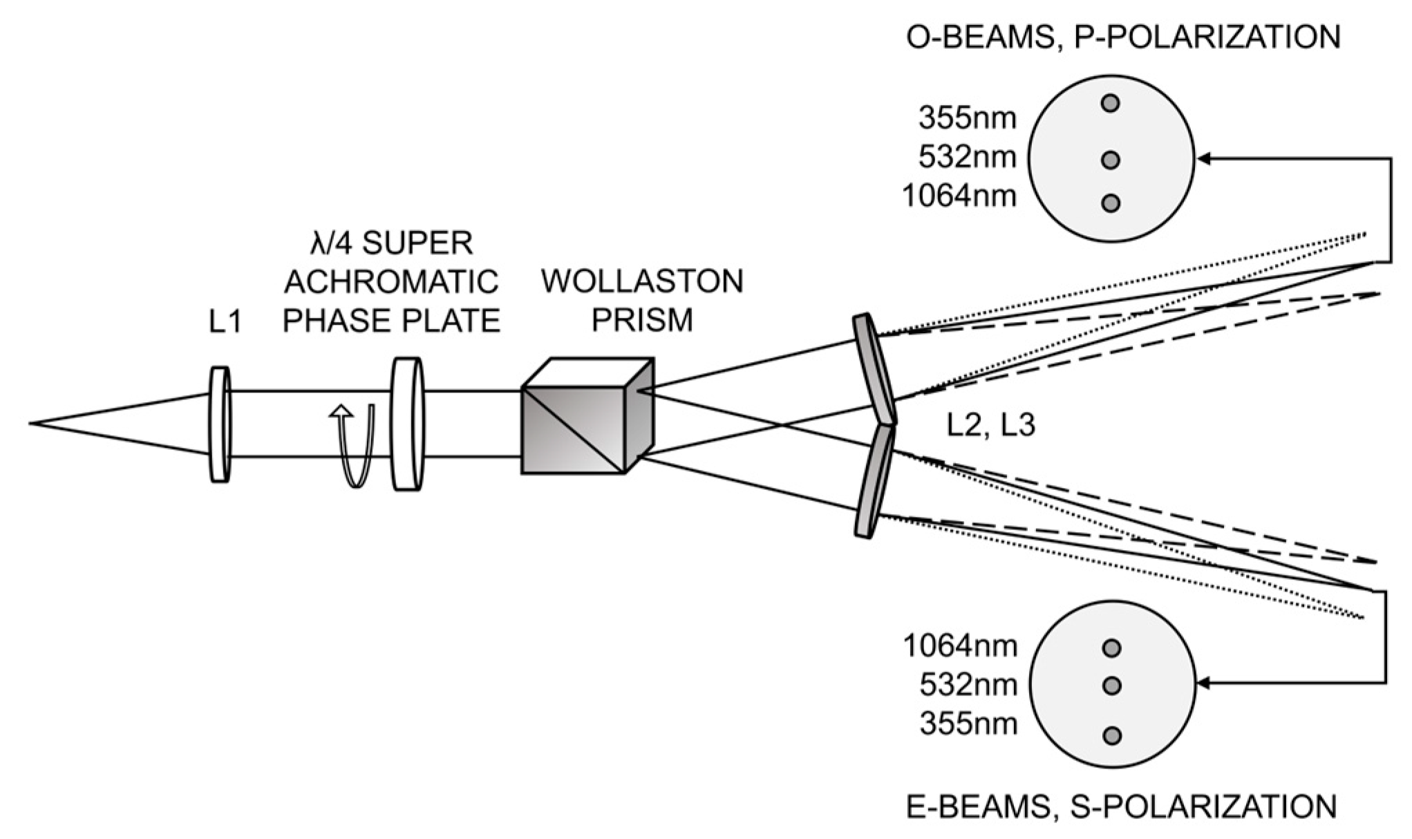
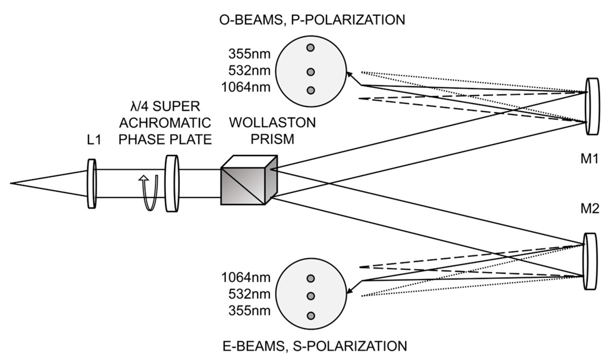
In Figure 4, the mirror-lens OSU variant is shown. The optical module becomes more compact. The problem of compensation for the chromatic aberration of the mirrors is absent. The background noise level created by the refracting lens surfaces is also much lower.

At the input of the unit, scattered radiation passes through the collimating lens L1 and is incident on the super-achromatic quarter-wave phase plate. After the plate, radiation is incident on the calcite (CaCO₃) Wollaston prism. Dispersed radiation is collected in the image plane of lenses L2 and L3 (mirrors M1 and M2), and through the quartz optic light guides (not shown in the figure), it enters the recording system (the block diagram of the recording system is not shown in the figures).

Selection of Optical Components of the OSU

At the stage of practical application of the MMPL, it is important to estimate the feasibility of the system from the viewpoint of current availability of the optical components. For this purpose, the behavior of suitable optical elements in the simplest OSU optical design was modeled. To solve this problem, the OSLO LT software version 6.1 was used. Only in rare cases of new optical glasses, it was necessary to use the optical ZEMAX 13 software version 2.

Based on catalogs of leading optics manufacturers, the variants of combinations of the collimating lens L1 and the focusing lenses L2 and L3 (variants A and B) are grouped in

Table 1. Variants of practical implementation of the spectral selection unit.

Variant	Collimating Lens Focal Length, mm Item # Glass	Focusing Lenses Focal Length, mm Item # Glass	Price, rel. Units
A	90 #64-838, Edmund Optics CaF2/Fused Silica/CaF2	180 #64-840, Edmund Optics CaF2/Fused Silica/CaF2	1.0
B	100 ACA254-100-UV, Thorlabs CaF2/Fused Silica	200 ACA254-200-A, Thorlabs N-SSK2/N-KZFS5	0.3
C	90 #64-838, Edmund Optics CaF2/Fused Silica/CaF2	180 Spherical mirrors	0.4

.

Table 2. Calculated image deviations at wavelengths of 355 and 1064 nm from the reference image plane at a wavelength of 532 nm.

Variant	355 nm Deviation, mm RMS Radius, μm	532 nm Deviation, mm RMS Radius, μm	1064 nm Deviation, mm RMS Radius, μm
A	–2.496 182	0 151	–1.205 120
B	+0.962 69	0 4	–0.123 65
C	+1.807 115	0 89	+0.522 66

presents the deviations of distances from the reference image planes calculated at a wavelength of 532 nm. At the top of the cells, the deviations of distances are given, and in the bottom, the corresponding root-mean-square radii of the image spots are presented.

Most optical materials have good transmission in the region of 1064 nm. However, the choice of optical materials for the region of 355 nm is noticeably limited. For the light guides, the application of fused silica with wide bandwidth in the UV–IR ranges is justified. To correct the chromatic lens aberration, doublet or triplet combinations of glasses should be used. This further narrows the range of choice of optical materials for the wideband lenses L1, L2, and L3.

The variant C (Figure 4) involves the use of the focusing mirrors instead of lenses. In the right column of the table, the prices for the collimation and focusing optics are given relative to the price of the variant A accepted for unity. The cells in the data table are divided into three levels: the focal lengths of the optical elements are indicated at the top; in the middle, the serial number of the manufacturer is given; and in the bottom, the combination of glasses according to the Schott catalog is presented.

In variant A, the UV-to-NIR corrected triplet lenses for the collimating lens L1 and the focusing lenses L2 and L3 are used. The specified triplets are corrected for the range of 193–1000 nm.

In variant B, the near-UV achromatic doublet is used for L1; for L1 and L2, they are the VIS achromatic doublets with transmission at a wavelength of 355 nm equal to about 0.73.

In variant C, the UV-to-NIR corrected triplet is used for L1, and the spherical mirrors M1 and M2 with a focal length of 200 mm are used instead of lenses L2 and L3.

3.2. Method of Optical Selection of the Polarization Components

The performance of the proposed configuration was checked using modeling. The aim of modeling was to determine the relative position of light guides at the output from the module depending on the focal lengths of the employed focusing lenses or mirrors.

For this purpose, direct calculations were carried out with the help of the mathematical package Mathcad_2001i and then were compared to the results of modeling of the optical OSU scheme using the OSLO LT optical modeling software. Results of the comparison showed insignificant deviations of the calculated data; therefore, it is sufficient to use direct calculations to solve this problem.

The proposed optical selection method is based on the birefringence and optical dispersion properties of the Wollaston prism inserted in the receiving lidar system. This allowed us to improve the lidar compactness and mobility.

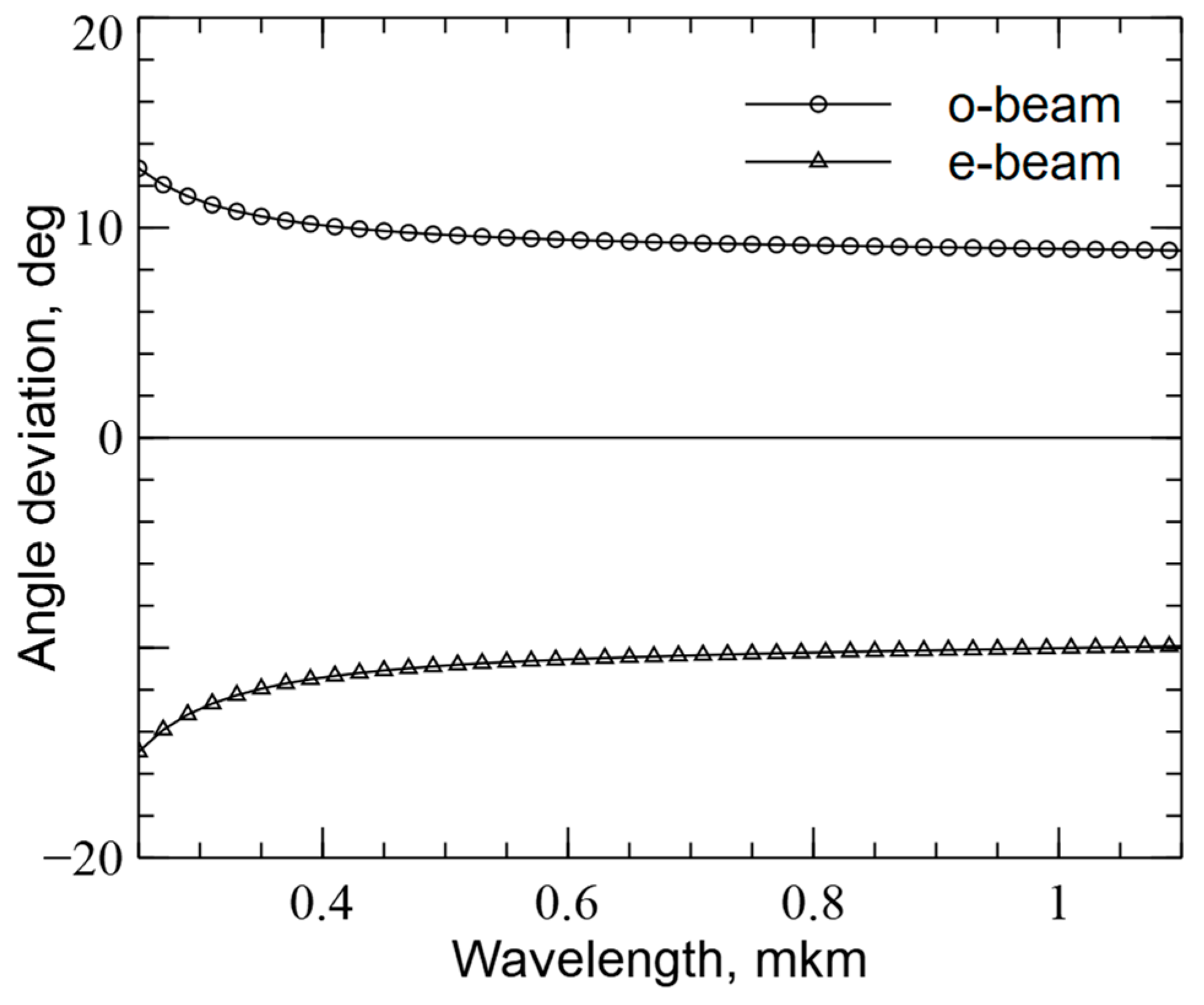
The results of modeling the radiation passage through the Wollaston prism are shown in Figure 5 and Figure 6.

In Figure 5, the angular dependences of the refraction of the ordinary (o-beam) and extraordinary (e-beam) components on the radiation wavelength are shown. The calcite crystal stands out among the birefringent crystals with its high dispersion level in the entire optical range.

The transmission range of the calcite Wollaston prism is 300–2300 nm. The production of the Wollaston prisms has well been established, and considerable experience of their practical application has been accumulated. The wavelength dependences of the refractive indices of the ordinary, $n_o\left(\lambda \right)$, and extraordinary, $n_e\left(\lambda \right)$, light beams passing through the calcite crystal are described by the Sellmeier equations:

$$n_o\left(\lambda \right)=\sqrt{1.73358749+\frac{0.96464345{\lambda }^2}{{\lambda }^2-1.94325203\times {10}^{-2}}+\frac{1.82831454{\lambda }^2}{{\lambda }^2-120}},$$

(10)

$$n_e\left(\lambda \right)=\sqrt{1.35859695+\frac{0.82427830{\lambda }^2}{{\lambda }^2-1.06689543\times {10}^{-2}}+\frac{0.14429128{\lambda }^2}{{\lambda }^2-120}}.$$

(11)

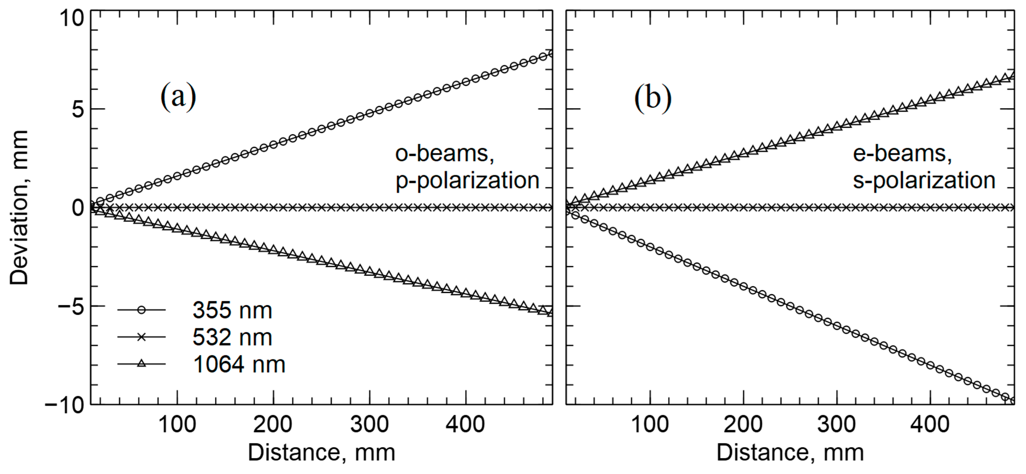
In Figure 6, the mutual positions of the cross-polarized beams are shown in the image plane depending on the focal lengths of the focusing lenses/mirrors.

On the left (Figure 6a), the o-beams and p-polarizations are shown, and on the right (Figure 6b), the e-beams and s-polarizations are shown for radiation at wavelengths of 355, 532, and 1064 nm. Calculations were carried out for a reference wavelength of 532 nm.

3.3. Methodology of the MMPL Experiment

A common practice in the technique of polarization sensing is the use of identical sets of different wave plates for both the transmitter and the lidar receiver. However, different plates have different transmission coefficients, which ultimately leads to difficulties in interpreting the results obtained. Therefore, here we propose the transition to one rotating wave plate in both the lidar transmitter and receiver in polarization measurements (with the MPL and MMPL).

We consider that the angular positions $\left\{ {\phi }_{INC}, {\phi }_{SCA}\right\}$ of the wave plates $R_{INC}$ and $R_{SCA}$ in the successive method of polarization measurements form the combination of the sample return forms ${\overline{A}}_m^n=m^n$; here $n=2$.

The robustness of the method of estimating the elements of the backscatter matrices depends on the choice of the angular states $\left\{ {\phi }_{INC}, {\phi }_{SCA}\right\}$. This problem was considered from the viewpoint of the MPL calibration in work [21]. The robustness of the method, its convergence rate, deviations of the estimates, and their behavior for low lidar returns were verified by the statistical method. For this purpose, the series of lidar returns of different levels were modeled.

Based on the results obtained, we consider that the combination of the angular positions $\left\{ {\phi }_{INC}, {\phi }_{SCA}\right\}$ of the $\lambda /4$ plates of the wave plates $R_{INC}$ and $R_{SCA}$ forms the sequence the same as in the nonlinear calibration problem. The fact that the direct and inverse problems of polarization sensing obey the well-known reciprocity (disambiguation) principle serves as the basis for this transition.

These are two optimal combinations: the fast combination with ${\overline{A}}_3^2$ = 9 and the slow combination with ${\overline{A}}_4^2$ = 16. The fast combination is $\left\{ {\phi }_{INC/SCA}\right\}=\left\{ 0,\pi 3/8,\pi 6/8\right\}$; here, the angles are in radians. The slow combination is $\left\{ {\phi }_{INC/SCA}\right\}=\left\{ 0,\pi 2/8,\pi 5/8,\pi 7/8\right\}$.

3.4. Method of Processing Measurement Results

At the final stage of the polarization experiment, it is necessary to estimate the elements of the full backscatter matrix from the data measured by the MMPL. This is the direct (linear) problem of polarization sensing. Here we first describe in complete detail the method of processing measurement data. Note that in the derivation of the method, we follow the paradigm indicated in the Introduction.

Thus, this method is universal for the MPL and MMPL. The main procedures of the method implemented in the software support for the experiments were repeatedly tested in various conditions. Note that the least squares core software of the method is the same for the lidar calibration problem and the problem of estimating the scattering matrix element. This has allowed us to verify the employed algorithms based on the reciprocity principle. In other words, if we calibrate the lidar as described in work [21], then direct measurements in the same layer must give the scattering matrix of the same form [16].

The method of estimating the elements of the backscatter matrix from the equations for the scattering matrix has been studied in sufficient detail. This is a linear problem for the elements of the backscatter matrix, and the method of its solution is independent of the choice of the sensing wavelengths.

Assume that photon counting is described by the Poisson statistics [24]. This is the so-called additional information. Using this assumption accepted in experimental research, we take the estimates of the mean values in a sample equal to the mean values themselves, and the estimates of the measurement errors equal to the estimates of the mean values themselves. The optimal solution is obtained based on the generalized least squares (GLS) method [25,26,27,28,29,30,31]. The procedure of obtaining estimates for the backscatter matrix elements is described by Formulas (A6)–(A14).

4. Results and Discussion

In terms of the modified instrumental vectors, the polarization lidar equations of the MMPL have been derived. The polarization equation for the scattering matrix was derived and the method of its solution was proposed. The method is characterized by the fact that the minimum estimates of the functional are independent of the form of the distribution of random variables. The estimates of the matrix elements are unbiased and effective.

In this work, the principles of MMPL design have been analyzed. We describe the new procedure of measuring the full scattering matrix with the multiwave polarization lidar. The optical block diagram of the MMPL has been presented.

This paper is the continuation of our previous work in which the new approach to the problem of calibration of the matrix polarization lidar (MPL) parameters is considered [21]. These works describe solutions to problems allowing one to proceed to a new, modern level of polarization research.

The variants of the practical implementation of the optical selection unit have been given. It was shown that the use of the standard calcite crystal Wollaston prism simultaneously can solve the problems of selection of the cross-polarized signal components and of the wavelength selection of signals. It has been shown that this challenge can be solved within the framework of simple solutions.

It was shown that the mirror-lens variant allows expenses on the collimating and focusing optics to be decreased by a factor of about 2.5. The compromise variant is also possible that allows these costs to be reduced by a factor of 3.3; however, in this case the radiation transmission at a wavelength of 355 nm is reduced. These variants are only estimates; for example, the effect of lens coatings on the radiation transmission was not taken into account in our calculations.

5. Conclusions

In the present work, it has been shown that new solutions in the methods of optical selection of the polarized radiation components received in the experiment and the methods of carrying out polarization studies together with new solutions in experimental data processing methods can solve the complex problem of the MMPL development. It has been shown that this problem can be solved within the framework of simple solutions. Thus, it has been shown that the proposed MMPL is structurally simple, compact, and can be used in mobile polarization lidar systems.