Article

Hybrid Post-Processing on GEFSv12 Reforecast for Summer Maximum Temperature Ensemble Forecasts with an Extended-Range Time Scale over Taiwan

by
Malasala Murali Nageswararao
1,2,*,
Yuejian Zhu
2,
Vijay Tallapragada
2 and
Meng-Shih Chen
3
1
The Cooperative Programs for the Advancement of Earth System Science (CPAESS), University Corporation for Atmospheric Research (UCAR) at NOAA/NWS/NCEP/EMC, College Park, MD 20740, USA
2
NOAA Center for Weather and Climate Prediction(NCWCP), National Center for Environmental Prediction (NCEP), Environmental Modeling Center (EMC), University Research Court, College Park, MD 20740, USA
3
Central Weather Administration, Taipei 100006, Taiwan
*
Author to whom correspondence should be addressed.
Atmosphere 2023, 14(11), 1620; https://doi.org/10.3390/atmos14111620
Submission received: 15 September 2023 / Revised: 20 October 2023 / Accepted: 26 October 2023 / Published: 29 October 2023
(This article belongs to the Special Issue Heat Waves: Perspectives from Observations, Reanalysis and Modeling)

Abstract

:
Taiwan is highly susceptible to global warming, experiencing a 1.4 °C increase in air temperature from 1911 to 2005, which is twice the average for the Northern Hemisphere. This has potentially led to higher rates of respiratory and cardiovascular mortality. Accurately predicting maximum temperatures during the summer season is crucial, but numerical weather models become less accurate and more uncertain beyond five days. To enhance the reliability of a forecast, post-processing techniques are essential for addressing systematic errors. In September 2020, the NOAA NCEP implemented the Global Ensemble Forecast System version 12 (GEFSv12) to help manage climate risks. This study developed a Hybrid statistical post-processing method that combines Artificial Neural Networks (ANN) and quantile mapping (QQ) approaches to predict daily maximum temperatures (Tmax) and their extremes in Taiwan during the summer season. The Hybrid technique, utilizing deep learning techniques, was applied to the GEFSv12 reforecast data and evaluated against ERA5 reanalysis. The Hybrid technique was the most effective among the three techniques tested. It had the lowest bias and RMSE and the highest correlation coefficient and Index of Agreement. It successfully reduced the warm bias and overestimation of Tmax extreme days. This led to improved prediction skills for all forecast lead times. Compared to ANN and QQ, the Hybrid method proved to be more effective in predicting daily Tmax, including extreme Tmax during summer, on extended-range time-scale deterministic and ensemble probabilistic forecasts over Taiwan.

1. Introduction

Temperature, a critical weather component, measures how hot or cold the environment is. It significantly impacts various sectors, including the energy industry, aviation industry, communication pollution dispersal, and agriculture. Climate change has become the most severe scientific and social challenge in this country. The IPCC report [1] shows that in the last 50 years, the annual mean temperature has been increasing at a linear trend of about 0.13 °C per decade, almost double the rate of the past century’s increase. In recent decades, recurrent heat waves with extremely high temperatures have been observed across the globe, including Asia [2,3,4,5], the USA [6], and Europe [7]. With the escalating progression of global warming, heat waves are predicted to increase in frequency, intensity, duration, and spatial coverage [1,8]. Heatwaves are among the most dangerous natural hazards worldwide, leading to an increase in deaths and emergency hospital admissions. They particularly impact children, older people, and patients with chronic diseases [2,9]. The US National Weather Service has shown that the annual casualties due to heat waves were more than those caused by many dynamic natural disasters such as floods, hurricanes, lightning, and tornadoes (http://www.nws.noaa.gov/om/hazstats.shtml (accessed on 1 June 2023).
Several studies [8,10] have found that heat waves over East Asia are primarily associated with persistent high-pressure and anticyclonic circulation patterns that dynamically produce large-scale subsidence and, therefore, prolonged hot conditions at the surface level. Numerous studies [11,12] reveal that the western North Pacific subtropical high (WNPSH) is a vital component of the East Asian summer monsoon system. It plays a significant role in regulating this region’s summer monsoon rainfall and tropical storm activities. The anomalous WNPSH is a crucial source of extreme climate conditions, such as flooding, drought, and heat waves, over the East Asian region. The occurrence of heatwaves in East Asia is primarily due to variations in WNPSH and is also associated with El Niño–southern oscillation (ENSO) as well as the tropical Indian Ocean warming [8].
Taiwan is one of East Asia’s subtropical islands, making it susceptible to extreme weather and climatic changes brought on by global warming [13]. According to the IPCC assessment [14], the rise in the air temperature in Taiwan (1.4 °C) from 1911 to 2005 is nearly twice the increase (0.7 °C) in the Northern Hemisphere. Research [15] shows that in Taipei during 1994–2003, each 1 °C increase in surface air temperature above 31.5 °C led to an approximate increase of 9.3% in respiratory mortality, with a range of 4.1–14.8%. Meanwhile, each 1 °C increase above 25.2 °C led to approximately a 1.1% increase in cardiovascular mortality, within a range of 0.3–1.9% [15].
Extended-range forecasts are generally used to predict weather and climate extreme events such as heatwaves, cold waves, droughts, and floods. These forecasts can provide relevant weather information, such as the onset timing of the rainy season, the risk of extreme rainfall events, heat waves, etc. However, there is still a well-known gap in current numerical prediction systems for extended-range time scales. This gap exists between medium-range weather forecasts (up to 10 days) and seasonal climate predictions (longer than one month). The initial conditions of the atmosphere influence medium-range weather forecasts. In contrast, seasonal climate predictions are more influenced by slowly evolving surface boundary conditions, such as the sea surface temperature and soil moisture content [16]. Predictions on the extended-range time scales have progressed in some regions and seasons [17] despite the full potential of their predictability requiring further exploration.
In recent years, there has been a significant improvement in the accuracy of short- and medium-range weather forecasts worldwide, particularly in extra-tropical regions, which benefit from advanced numerical modeling. However, the same cannot be said for tropical areas such as monsoon regions, where prediction skills remain inadequate [18,19]. This can predominantly be attributed to the complexity of tropical processes. These are influenced by the interactions between the ocean, land, and atmosphere; atmospheric circulation; convection; as well as clouds and radiation. Precipitation and moisture also play a role in affecting different spatial and temporal scales. To enhance the prediction accuracy on this time scale in smaller regions such as Taiwan Island, global models need to be improved to better represent land–sea contrast and topography [20]. In addition to enhancing the global models, post-processing techniques are also crucial for improving extended-range forecasts in smaller regions. Post-processing techniques can be utilized to correct systematic errors in the model output, such as bias in the mean and variance of the forecast variables. Numerous studies [21,22,23] have shown that the post-processing of raw GCM forecasts is essential. Various post-processing approaches with varying complexities and statistical basis have been developed to calibrate raw GCM forecasts [24,25]. Computationally efficient approaches have been proposed due to their ease of implementation and low computation cost. These include the rank histogram calibration method [22], the “poor man’s ensemble” method [26], the analog method [27], the frequency match method (FMM; [28]), and the quantile mapping method [19,29]. However, these methods may not yield reliable and skillfully calibrated forecasts [30]. Data-driven models, such as machine-learning models, are increasingly being used in post-processing. Comparisons of these models demonstrated that their performance varies with study areas, GCMs, and evaluation metrics [25]. Therefore, there is no single, ultimate post-processing model [31,32]. To provide reliable and skillful forecasts, an effective post-processing approach is essential. This approach must be unbiased, reliable in ensemble spread, and at least as good as the climatology reference forecasts.
The NOAA NCEP has implemented the Global Ensemble Forecast System version 12 (GEFSv12) to support stakeholders for sub-seasonal forecasts, hydrological, and other meteorological applications [29,33,34,35]. This model provides consistent reforecast products for the period of 2000–2019, which are available on Amazon Web Services (AWS, https://registry.opendata.aws/noaa-gefs/ (accessed on 1 June 2023)) and accessible to the public. In this study, an Artificial Neural Network combined with quantile mapping (ANN-QQ; hereafter termed as Hybrid post-processing) based on a statistical post-processing technique is applied to NCEP GEFSv12 reforecast raw products for predicting summer (June through September; JJAS) surface air maximum temperature (Tmax) and associated extremes (Tmax ≥ 90th percentile of annual Tmax) on an extended-range time scale over Taiwan. The paper is organized as follows: a brief description of the data and analysis methodologies is given in Section 2. The results are discussed in Section 3, and the broad conclusions are presented in Section 4.

2. Data and Methodology

2.1. Data Used

The surface air maximum temperature (Tmax) products of the NCEP GEFSv12 over Taiwan island (21.5° N–26° N, 119.5° E–122.5° E) for reforecast period (2000–2019) have been obtained from Amazon AWS. These products are generated from initial conditions at 00 UTC daily, with forecasts leading up to 16 days for 5 ensemble members. The reforecast products extended up to 35 days with initial conditions set weekly at 00 UTC every Wednesday for 11 ensemble members [27]. GEFSv12 reforecast products based on the Global Forecast System version 15.1 (GFSv15.1). It uses the FV3 Cubed-Sphere dynamical core [36] with a horizontal resolution of ~25 km (C384 grid) and 64 hybrid vertical levels, with the top layer centered at 0.27 hPa (~55 km). A modified scale-aware convection parameterization scheme is incorporated into GEFSv12 model physics to mitigate the excessive cloud-top cooling and stabilize the model [37]. The Hybrid Eddy-Diffusivity Mass-flux (EDMF) scheme is utilized to simulate vertical mixing in the planetary boundary layer [38], and the GFDL-based cloud microphysics scheme is used for predicting five cloud species [33,34]. The Rapid Radiative Transfer Model (RRTM), developed at Atmospheric and Environmental Research, is used to estimate shortwave and longwave radiative fluxes [39]. Chun and Baik (1998) developed a scheme for convective gravity wave drag [40]. On the other hand, the GFS orographic gravity wave drag and mountain blocking schemes are based on Alpert’s (1988) study [41]. A two-tiered approach is used to derive the SST boundary conditions, which account for the day-to-day variability of sea surface temperature (SST) and near sea surface temperature (NSST), respectively [42,43,44]. The GEFSv12 forecast system uses SKEB [45,46] and SPPTs [47,48] to represent model uncertainty. Further details on the configuration and impacts of the individual components can be found in the work of Zhou [33,34].
In this study, we used the GEFSv12 Tmax reforecast products. These are based on 00 UTC initial conditions every day and provide forecasts for a lead time of 1 to 16 days with 5 members. The reforecast data are available in grib2 format at 3 h intervals at 0.25° resolution for the first 10 days of forecasts. Beyond these 10 days, the data are available at 6 h intervals and at a resolution of 0.5°. For consistency, forecasts from Day-1 to 10 are considered to have the same horizontal resolution as forecasts from Day-11 to 16. The maximum 2 m air temperature (Tmax) over Taiwan for the period from 2000 to 2019, obtained from the ECMWF Reanalysis version 5 (ERA5) (https://cds.climate.copernicus.eu/cdsapp#!/dataset/reanalysis-era5-single-levels?tab=form (accessed on 1 June 2023), was used as a reference for evaluating the performance of GEFSv12. This evaluation focuses on summer Tmax and associated extreme events of Tmax (daily Tmax exceeding the 90th percentile) over Taiwan, with forecast lead times from Day-1 to 16 [49].
The ERA5 reanalysis dataset, based on a sophisticated weather model and including a wealth of data types, provides globally distributed weather variables at 30 km resolution. It employs an assimilation system using ground, ocean, satellite, and atmosphere observations, making it regarded as a proxy for regional observations [49]. In 2022, Lee and his team evaluated the capability of ERA5 data to accurately represent rainfall trends in Taiwan and discovered that it effectively identified significant, localized rainfall events [50]. Similarly, a 2020 research study by Mostafa Tarek and associates utilized ERA5 data as a benchmark for hydrological simulations in North American catchments and found its results to be on par with those derived from observation-based models [51]. Velikou and team, in their 2022 publication, confirmed the precision of ERA5 data in representing both average and peak temperatures across Europe [52]. Additionally, McNicholl and colleagues in 2021 stated that ERA5 data provide trustworthy estimates of weather conditions even in areas where on-the-ground measurements are unattainable [53]. These studies demonstrate the credibility of the ERA5 reanalysis dataset when used to create calibration models and serve as a benchmark for assessing the efficiency of raw and calibrated predictions.

2.2. Calibration Methods

2.2.1. Quantile Mapping

A suitable statistical post-processing technique is highly required to calibrate any GCM raw forecast products based on the reforecast period uncertainty for skillful forecast guidance and to increase its usability. In this study, the quantile mapping post-processing technique is used as a benchmark calibration method for evaluating the Artificial Neural Network (ANN) and the ANN combination with quantile mapping (ANN-QQ, hereafter mentioned as Hybrid). These calibration methods on NOAA GEFSv12 reforecast products for deterministic and ensemble probabilistic forecasts of summer Tmax and its extremes on an extended-range time scale over Taiwan with Day-1 to 16 forecast lead times have been evaluated against ERA5 reanalysis.
The QQ method, also known as histogram equalization or rank matching [11,19,54], is used to statistically transform model data into bias-corrected data to increase the usability of model products after calibration. The daily Tmax statistics for ERA5 reanalysis and GEFSv12 reforecasts were determined separately for each lead time (Day-1 to Day-16) and grid point of Taiwan. This calibration method is independently applied to each of the five ensemble members and each forecast lead time. To enlarge the sample size, a 31-day moving window is utilized, positioning the forecast day at the center. This results in a sample size of 620 time steps (31 days × 20 years) for each day and each lead time forecast at a grid point. For the gridpoint on 1 June 2000 with a Day-1 forecast lead time, the sample of daily Tmax from 17 May to 16 June from ERA5 and GEFSv12 reforecast period was used. The same procedure is independently implemented for each lead time and ensemble member at a grid point to approximate the daily Tmax intensity distributions from ERA5 and GEFSv12 reforecasts for each day from 1 June to 30 September. This technique employs the empirical probability distributions of ERA5 and GEFSv12 Tmax values to generate a calibrated output. The bias-corrected value for the Tmax forecast of the GEFSv12 model (Q) can be calculated by taking the inverse of the cumulative distribution function (CDF) of ERA5 values ( C D F E R A 5 1 ) at the probability corresponding to the raw GEFSv12 output CDF ( C D F G E F S v 12 ) at a particular value ( F t ).
Q = C D F E R A 5 1 C D F G E F S v 12 F t
The technique of quantile mapping involves a transformation between CDFs of the ERA5 and GEFSv12 models. The Leave-one-out Cross-Validation (LOOCV) procedure is implemented. The raw and QQ-calibrated forecasts are referred to as Raw-GEFSv12 and QQ-GEFSv12, respectively.

2.2.2. Artificial Neural Network (ANN)

The IPCC report [15] emphasizes the challenge meteorologists face in forecasting temperature changes due to global warming. The complexity and non-linearity of atmospheric variables, such as temperature fluctuations, make extended-range predictions quite complicated. A study [55] indicates that a method based on Artificial Neural Networks (ANN) provides more precise temperature prediction compared to conventional techniques due to its exceptional ability to handle the complex non-linearities of the atmosphere. This method surpasses statistical approaches that often require assumptions about data, such as normal distribution or data immutability, providing a superior way to detect discrepancies. The limitations of standard temperature prediction involve assumptions of linear connections between variables, which can occasionally complicate results [56]. Conversely, ANNs provide a robust tool for swift data processing inspired by biological neurons’ parallel processing. Interlinked neurons in ANN can handle complex situations and offer more precise temperature forecasts than traditional statistical approaches. Significantly, ANNs can adapt, permitting model weight adjustments to learn the relation between input and output from existing data directly [56]. ANNs have the ability to minimize training times and data requirements compared to other statistical methods. They can establish a correlation between inputs and outputs to forecast outcomes. As a data-centric approach, ANNs can discern non-linear associations between inputs and outputs without resolving intricate partial differential equations. This makes it an optimal tool for predicting temperatures, as shown in many studies using atmospheric data [57,58,59,60]. This study implements an ANN calibration method on GEFSv12 reforecast products for summer Tmax and associated Tmax extremes over Taiwan for all forecast lead times (Day-1 to 16).
ANNs can be either single-layer or multi-layer. The single-layer model directly connects each input and output unit without interconnections among input units. The more complex multi-layer model, however, does interconnect its input and output units [61,62]. The Back Propagation Neural Network (BPNN) uses the gradient descent method to minimize the discrepancy between the intended target and the actual outcome. This is a widely used design in Artificial Neural Networks (ANN) [63,64]. This type of ANN is constructed, assessed, and accuracy tested. Hecht-Nielsen undertook a study using double-cross-validation to find the perfect number of hidden neurons in a single hidden layer to avoid overfitting. However, an ANN’s effectiveness heavily depends on the training data and parameters like initial weights, learning pace, momentum, epoch, and activation functions. Thus, to achieve the best performance, the structure of the ANN should be custom designed to match the characteristics of the dataset [65]. In this study, pre-processing techniques were used to identify and eliminate outliers, reduce noise, and normalize the range of inputs and outputs for the daily Tmax from the 5 ensemble members of GEFSv12. The Neural Network Toolbox in MATLAB was used to train, visualize, and simulate ANNs. To determine the optimal ANN structure for a particular day forecast, a double cross-validation procedure was employed. This involved leaving out one datapoint from the 620 sample data and fitting the ANN model to the remaining data in a cross-validation mode. The performance of each iteration was monitored using metrics such as Mean Square Error (MSE) and Root Mean Squared Error (RMSE), while the number of hidden neurons increased from 1 to 20.
Many research studies [64,66] have shown that when the number of hidden neurons is increased, the MSE and RMSE decrease for both training and testing data. However, after a certain point, the MSE and RMSE decrease for training but increase for testing. This study also indicates that after a certain point, the errors in testing data will continue to rise without much change in the training data. To ensure that the training, testing, and validation sets are evenly distributed across different classes and to avoid any potential issues that may arise from having similar or sequential data in the sets, the optimal number of neurons for the ANN model was determined by randomizing the pooled dataset. This resulted in a best-hidden layer size of 7. In the context of a Backpropagation Neural Network (BNN), randomization helps to prevent the algorithm from quickly converging to local minima by introducing oscillations.
To optimize the ANN, the Min-Max transformation is applied to input and output values to speed up the training process, avoid saturation, and reduce the chances of becoming stuck in local optima. This transformation shifts the data into the range [−1, 1] through the following equation:
X i , s c a l e d = X i X m i n X m a x X m i n
where X i is the original input value. After the ANN simulation, the transformed values are converted back to their original values using various transfer functions. Johnstone and Sulungu [67] discuss the most commonly used transfer functions, such as linear, hyperbolic tangent sigmoid, and logistic sigmoid, which are suitable for problems with non-linearity. These transfer functions enable the ANN to accurately convert the transformed values back to their original form. In this study, a feed-forward Backpropagation Neural Network with 7 hidden neurons and a hyperbolic tangent sigmoid transfer function was implemented using the MATLAB ANN toolbox and the Levenberg–Marquardt training algorithm for deep learning of summer Tmax over Taiwan. This choice of transfer function is effective for temperature prediction, as it is a non-linear, differentiable, and monotonic function that yields better training performance for multi-layer neural networks. In this study, a basic ANN is created using the components outlined in Table 1.
For summer Tmax forecasts over Taiwan, the ANN calibration method is applied to each forecast lead time at a grid point independently using a 31-day moving window with 620 sample data (31 days × 20 years). The forecast day is the center of the 31-day moving window. The Leave-one-out Cross-Validation (LOOCV) procedure has been implemented to calibrate the outputs of the GEFSv12 using ANN. The resulting calibrated outputs are referred to as ANN-GEFSv12.

2.2.3. Hybrid Post-Processing

The QQ technique, described in Section 2.2.1, was used to improve summer daily Tmax and associated Tmax extremes in Taiwan by applying it to the ANN-GEFSv12 output. The LOOCV procedure was used to evaluate the performance of the Hybrid statistical post-processing method. A visual representation of the methodology used in this study is presented in Figure 1. The predictive accuracy of the different calibration methods for deterministic and ensemble probabilistic forecasts of Tmax and associated extremes was compared using standard skill metrics.

2.3. Analysis Procedure

The accuracy of Raw, QQ, ANN, and Hybrid methods in predicting summer daily Tmax over Taiwan for Day-1 to 16 forecast lead times during the reforecast period (2000–2019) was evaluated against ERA5 using standard skill metrics such as mean bias (MB), Root Mean Square Error (RMSE), correlation coefficient (CC), and Index of Agreement (IOA). The probability distributions of the Raw and all three calibration methods were compared with ERA5 by pooling all grid points and 5 ensemble members for each forecast lead time separately. The spatial distribution of summer (JJAS) Tmax extremes over Taiwan was analyzed, taking into account the average frequency of Tmax extremes from all five individual members for each forecast lead time separately. The performance of Raw and all three calibration methods in predicting summer Tmax extremes against ERA5 was evaluated using a contingency table and associated statistical categorical skill scores, such as Accuracy (ACC), Frequency Bias (BIAS), Probability of Detection (POD), False Alarm Rate (FAR), Success Ratio (SR), Threat Score (TS), and Equitable Threat Score (ETS). A performance diagram has been created to illustrate the statistical categorical skill scores of Raw and all calibration methods in depicting summer daily Tmax extremes. This diagram measures the geometric relationship between Frequency Bias, SR, FAR, POD, and TS [68].
Probabilistic forecasts are essential for providing more accurate and reliable weather and climate predictions, as they are better able to capture the inherent uncertainty of extreme events. To evaluate their accuracy, metrics such as reliability, resolution, Brier score (BS), Brier skill score (BSS), and receiver operating characteristic (ROC) curve are used. These metrics are invaluable for climate risk management in various sectors. The Brier score measures the accuracy of probabilistic forecasts in binary situations and ranges from 0 to 1, with 0 being the perfect score. The Brier skill score (BSS) is used to compare the accuracy of a probabilistic forecast to a reference/climatological forecast. A BSS of 1 indicates an accurate forecast, while a BSS of 0 or lower suggests that the forecast is less reliable than the reference [69,70]. The reliability and resolution of an ensemble probabilistic forecast of a particular category are two distinct characteristics [71]. The reliability of an ensemble probabilistic forecast is the accuracy of the predicted class/interval of outcomes compared to the actual distribution of observations. A perfectly calibrated forecast has a reliability of 0, while a scale from 0 to 1 measures the reliability of a forecast, and 1 represents the worst reliability. The resolution of a forecast is a measure of its accuracy in predicting the frequency of an event. A resolution of 0 indicates that the forecast is either always the same or completely random, while a resolution equal to the uncertainty means that all uncertainty has been accounted for. The receiver operating characteristic (ROC) curve plots the False Alarm Rate (FAR) on the x-axis against the Probability of Detection (POD) on the y-axis. A forecast with skill will have a curve above the diagonal line, while a forecast below the line is worse than a climatological or reference forecast. An accurate forecast will be close to the ideal upper left corner [72].

3. Results

This study applied various calibration methods to NOAA NCEP GEFSv12 reforecasts to improve the predictability of summer daily Tmax and associated Tmax extremes over Taiwan. The performance of these methods was evaluated using standard skill metrics for deterministic and ensemble probabilistic forecasts. The results are discussed in the following subsections.

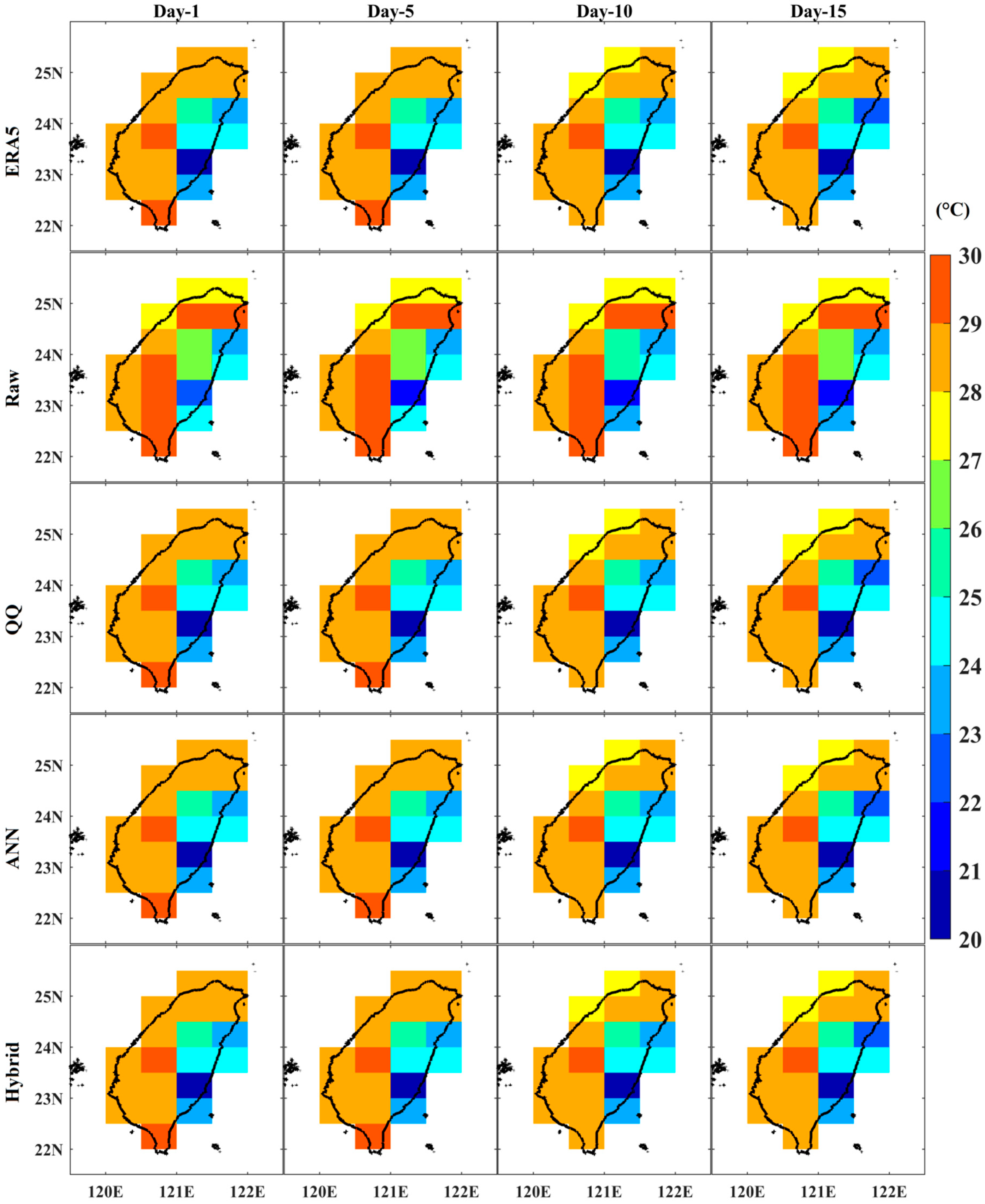
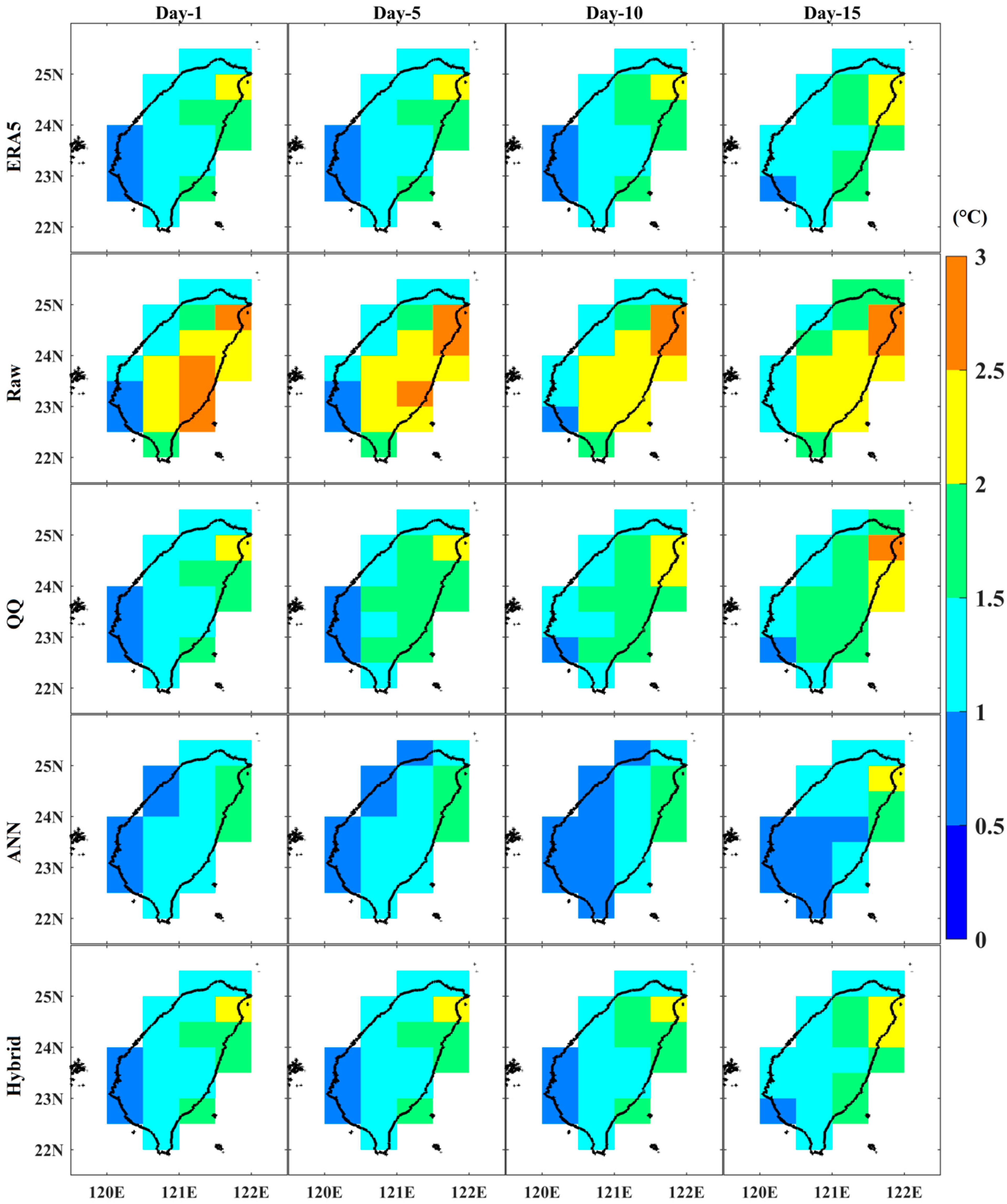
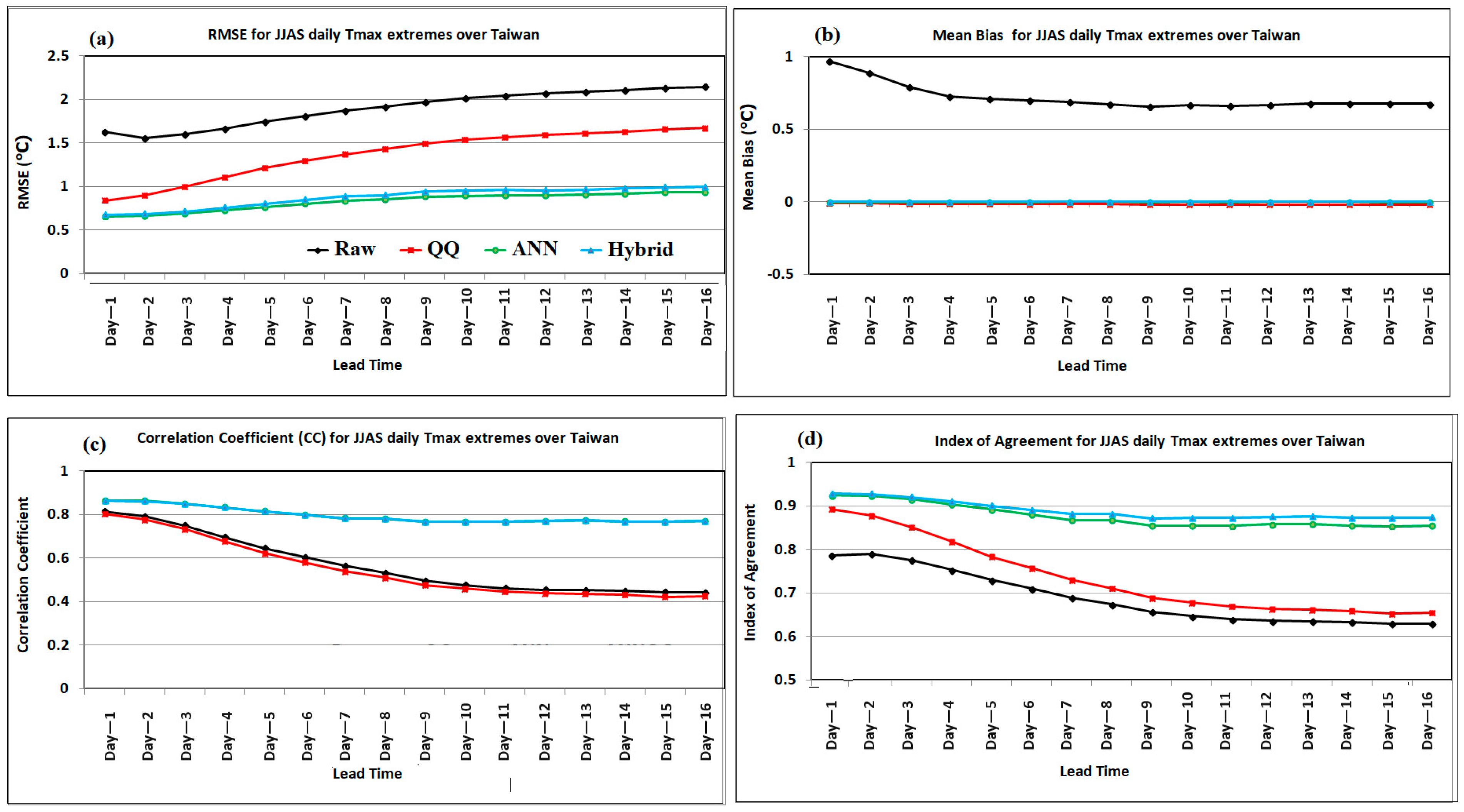
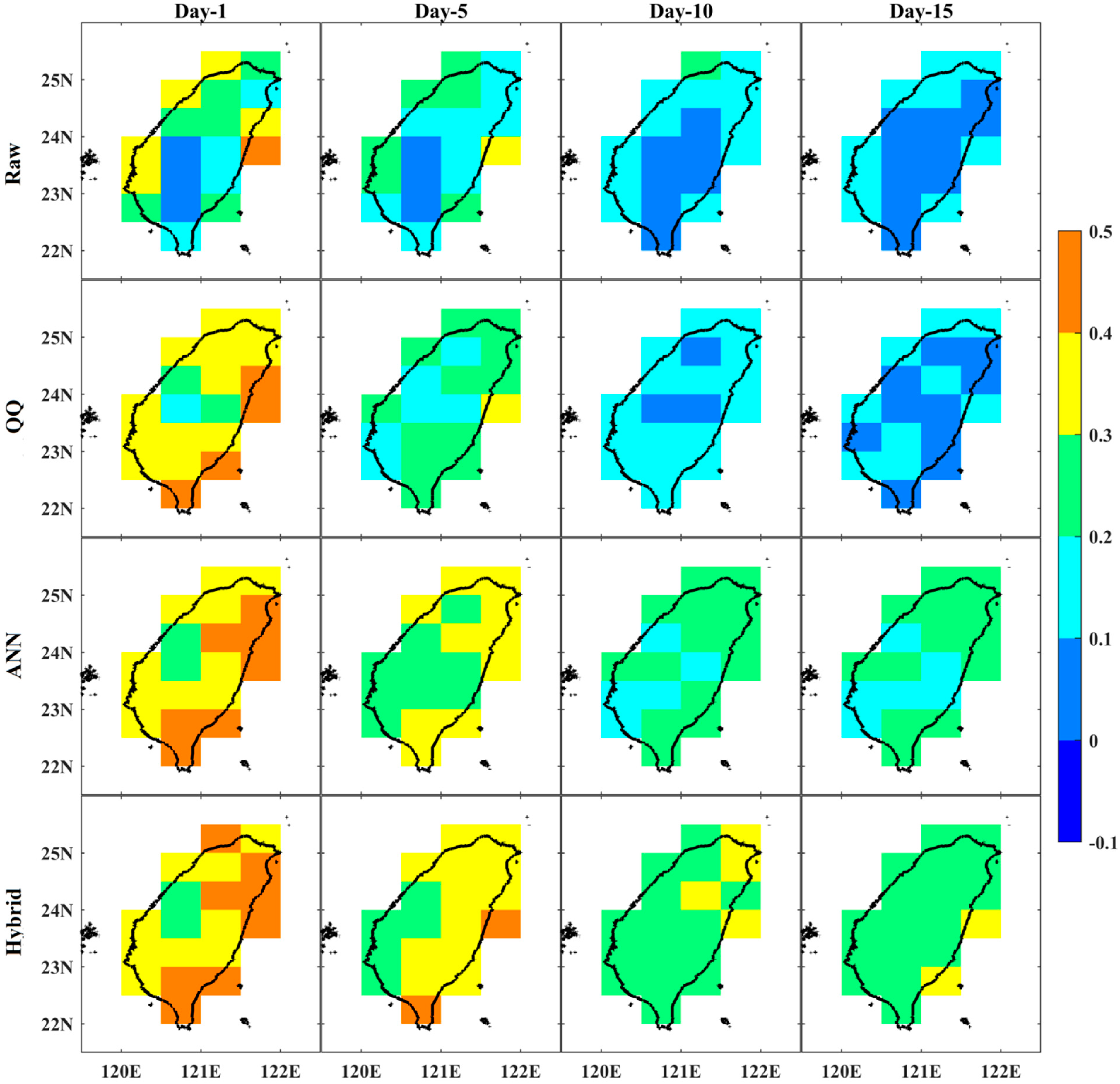
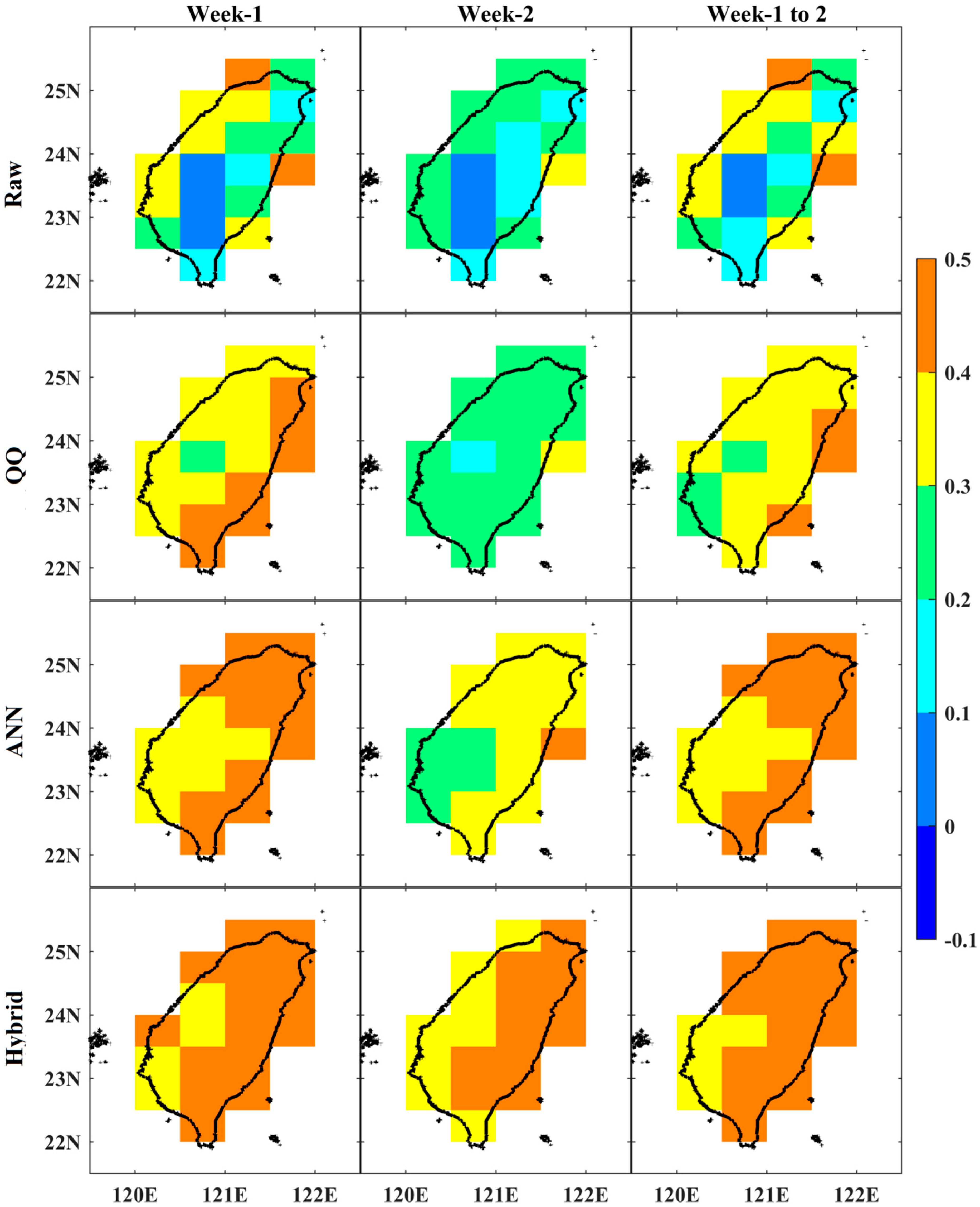
3.1. Prediction Skill of Raw, QQ, ANN, and Hybrid Post-Processing Methods for Summer Daily Tmax over Taiwan

The performance of raw and three calibration methods (ERA5, QQ, ANN, and Hybrid) for predicting summer (JJAS) daily Tmax over Taiwan for 2000–2019 was evaluated by analyzing the spatial patterns of the climatological mean at forecast lead times of Day-1, 5, 10, and 15 (Figure 2). Both Raw-GEFSv12 and ERA5 display similar spatial patterns of summer daily Tmax over Taiwan for all forecast lead times. However, GEFSv12 exhibits a warm bias in most parts of the country. The daily Tmax from ERA5 is lower in the east and progressively increases towards the west, a trend that is similarly observed in GEFSv12. The highest summer Tmax is observed in the southernmost region of Taiwan. The GEFSv12 forecasts for all lead times confirm this. All calibration methods notably reduced the warm bias in most parts of Taiwan, resulting in a Tmax climatological mean similar to ERA5 for all forecast lead times.
The spatial patterns of IAV of summer Tmax over Taiwan from GEFSv12 and ERA5 are similar across all forecast lead times (Figure 3). The GEFSv12 model tends to overestimate the IAV of summer Tmax in most parts of the country for all forecast lead times. The IAV of Tmax is higher in the northeastern part of the country, and this is accurately represented in the GEFSv12 forecasts for all lead times. All three calibration methods successfully reduced the overestimation in IAV of Tmax over Taiwan. The spatial patterns of the IAV of Tmax were found to be similar to those of ERA5 for all forecast lead times. The ANN method slightly underestimated the IAV of Tmax in most parts of the country, while the QQ and Hybrid methods accurately captured the magnitude of the IAV of Tmax over Taiwan for all forecast lead times. The Hybrid method of capturing the IAV of Tmax in Taiwan is more effective than the QQ method, especially for longer lead time forecasts (Figure 3).
The QQ method has the advantage of adjusting the Tmax probability distribution to the observed data, particularly in the extreme tails, to account for IAV. The spatial patterns have been improved; however, the temporal patterns remain unchanged. Deep learning combined with the QQ method has been found to be effective in capturing temporal patterns, IAV, and climatological patterns. The Hybrid method has been seen to be more successful than the QQ and ANN methods.
The Raw-GEFSv12 model showed a high RMSE in predicting summer daily Tmax in the eastern parts of Taiwan for all forecast lead times (Figure 4). The patterns of RMSE were akin to the IAV patterns, showing elevated values in regions with high IAV. The RMSE increased with lead time. All three calibration methods effectively reduced the RMSE in most parts of Taiwan for all forecast lead times. The RMSE of the QQ method increases for longer lead times, while the ANN and Hybrid methods demonstrate substantial improvements. The comparison between the methods reveals that the RMSE of ANN and Hybrid methods is lower than that of the QQ method for all forecast lead times, particularly in the eastern parts of the country (Figure 4).
The GEFSv12 shows a high Index of Agreement (IOA) (>0.8) for predicting summer daily Tmax in northwestern Taiwan, decreasing to >0.5 in the southeast (Figure 5). However, the IOA is lower for all forecast lead times in the central part of the country. The IOA of GEFSv12 for summer daily Tmax generally decreases with increasing forecast lead time in most areas. However, the implementation of calibration techniques has notably enhanced the IOA in predicting Tmax over Taiwan across all forecast lead times. The ANN method has an IOA range of 0.7 to 1, which is higher than the QQ range of 0.5 to 1. The accuracy of the forecasts for Tmax in all parts of Taiwan produced by ANN is significantly higher for longer lead times. Conversely, the IOA from QQ deteriorates with an increase in lead time, primarily due to the greater magnitude of errors in the forecasts. However, the Hybrid method yields a higher IOA value (0.8–1) than the other two methods, making it the most reliable for predicting daily Tmax during the summer over Taiwan across all forecast lead times. Hybrid methods of predicting Tmax demonstrate more reliable results across the majority of the country compared to ANN and QQ for all forecast lead times (Figure 5).
The performance of the Raw and all three calibration methods in predicting Tmax over Taiwan for the reforecast period were evaluated using RMSE, mean bias, correlation coefficient, and Index of Agreement (Figure 6). The results demonstrated that the RMSE increased proportionally with the forecast lead time. The Raw displayed the highest RMSE, fluctuating between 1.5 and 2.5 °C. Yet, the usage of calibration techniques including QQ (0.8–1.2 °C), ANN (0.6–1 °C), and Hybrid (0.6–1 °C) notably reduce the RMSE across all forecast lead times (Figure 6a). The comparison of the methods reveals that ANN and Hybrid have similar RMSE values, which are much lower than QQ for all forecast lead times (Figure 6b). The warm bias of 0.6–1 °C over Taiwan during the summer season was successfully reduced to nearly 0 °C by all calibration methods. The GEFSv12 exhibits a distinct correlation with Taiwan’s daily summer Tmax for Day-1 forecasts, showing a high correlation value of more than 0.8. However, the correlation tends to diminish with an increase in lead time, falling to 0.4 (refer to Figure 6c). No improvement was observed in the correlation coefficient when the QQ method was used compared to the Raw products. Both the ANN and Hybrid calibration methods significantly improved the correlation coefficient (r > 0.79) for all forecast lead times. The Hybrid method yields the same correlation coefficient values as the ANN for all forecast lead times. However, for longer lead times, both the ANN and Hybrid methods show a significant improvement in the correlation coefficient (Figure 6c). The IOA of GEFSv12 in predicting Tmax over Taiwan is highest for shorter lead times (0.8) and decreases to 0.6 as the forecast lead time increases (Figure 6d). All calibration methods enhance the IOA at each forecast lead time. The Hybrid method exhibits the maximum IOA (0.92), outperforming both the ANN (0.88) and QQ (0.9) methods. The Hybrid method consistently produced higher IOA values compared to the ANN across all forecast lead times, as depicted in Figure 6d. The Hybrid calibration method exhibited higher IOA values than the QQ method for all forecast lead times (Figure 6d). This increase in accuracy is particularly beneficial for longer lead time forecasts, which can greatly aid climate management in various regional sectors, such as Taiwan.
The probability distribution (PDF) of summer daily Tmax over Taiwan was calculated from all five ensemble members and all grid points of Taiwan daily Tmax values pooled for ERA5, Raw, and each calibration method for the study period and selected lead time forecasts (Day-1, 5, 10, and 15). The results are shown in Figure 7. The Raw data PDF of the daily maximum temperature during summer is more right-skewed than the ERA5 data across all forecast lead times. This suggests that there is a higher frequency of extreme Tmax days in the Raw data compared to the ERA5 data. These findings are illustrated in Figure 7. The calibration methods were well-adjusted for the probability distribution of summer daily Tmax over Taiwan to ERA5 for all the forecast lead times. The QQ method was found to be more effective than the ANN. The Hybrid method proved to be the most effective for adjusting the PDF of summer daily Tmax over Taiwan, according to ERA5 data. It performed better than both the QQ and ANN methods in aligning the summer daily Tmax PDF with the ERA5 data.

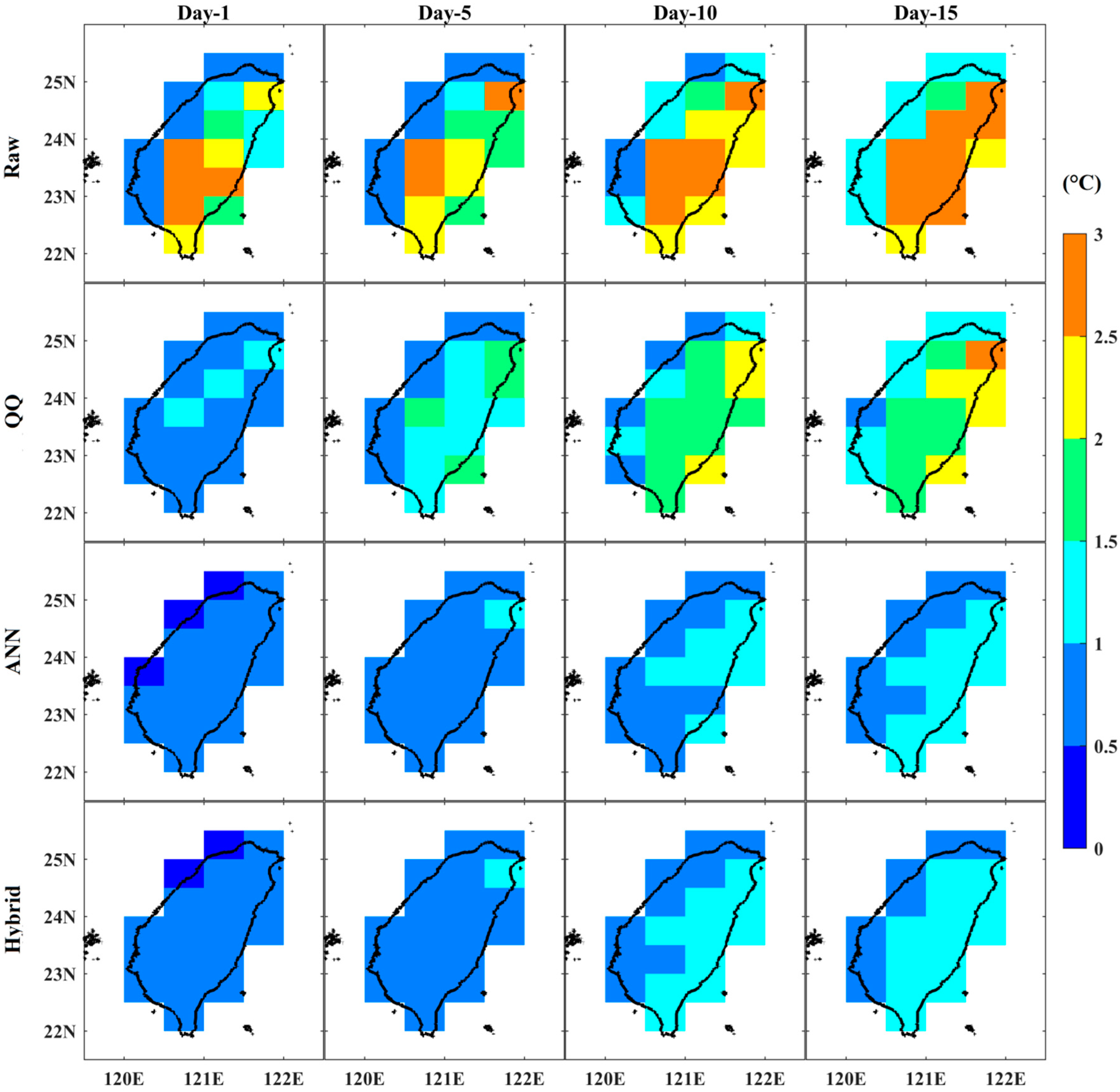
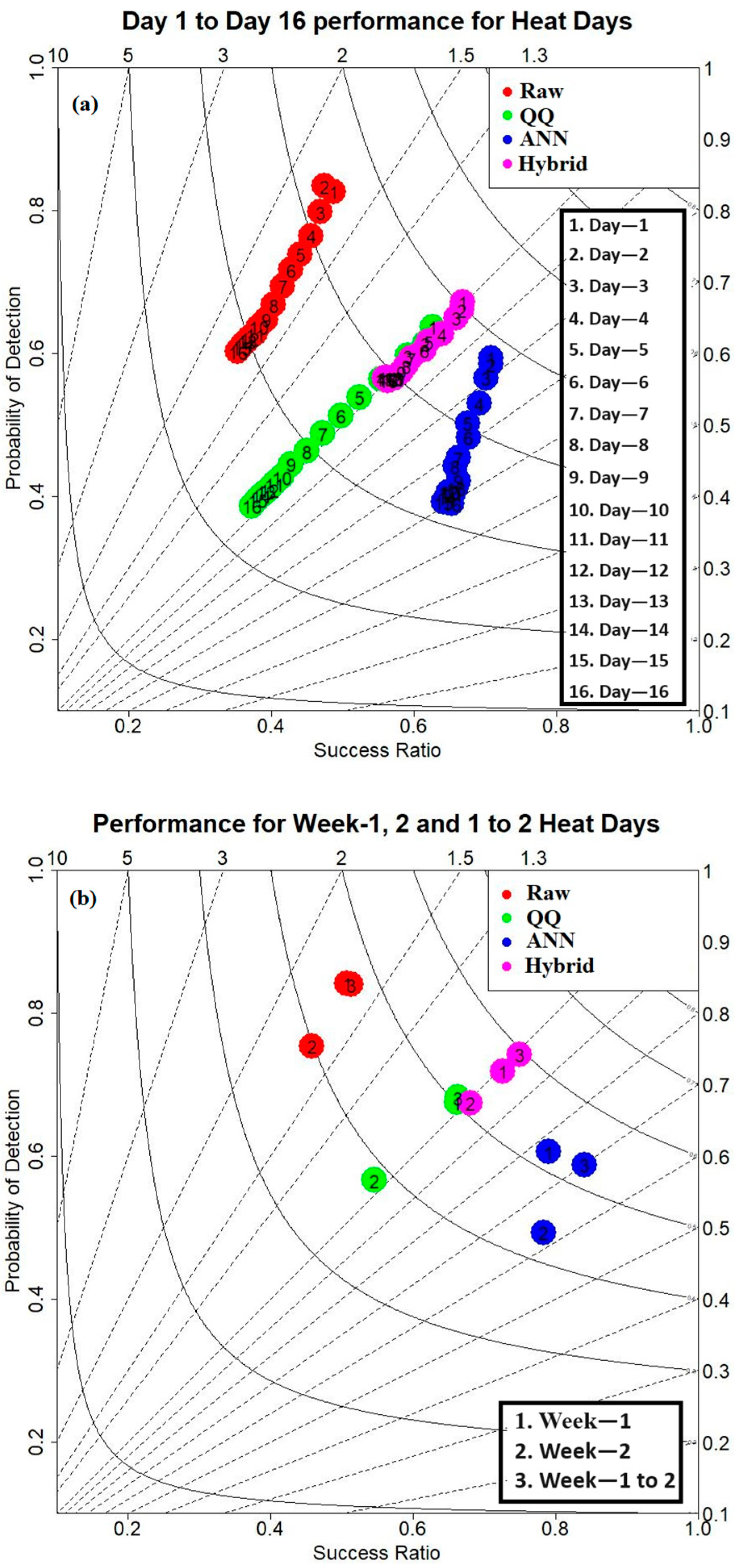
3.2. Statistical Categorical Skill Scores for Summer Daily Tmax Extremes over Taiwan from Raw, QQ, ANN, and Hybrid Methods

Statistical skill scores (e.g., POD, FAR, ACC, SR, TS, ETS) were computed for the 2000–2019 reforecast period for Taiwan’s summer daily Tmax extreme days (Tmax > 90th percentile of annual Tmax) from Day-1 to 16. The ETS of GEFSv12 for summer daily Tmax extremes is higher in coastal areas than in interior regions of Taiwan (Figure 8). The ETS values decrease with the increasing forecast lead time. All calibration methods tested showed an improvement in the ETS score for summer daily Tmax extremes over Taiwan for all forecast lead times. Raw and all three calibration methods for summer daily Tmax over Taiwan indicate a decrease in ETS score with increasing forecast lead times. However, the ANN method yields a higher ETS score than the QQ calibration method. The Hybrid method yields the highest ETS score than ANN and QQ for all forecast lead times (Figure 8).
The ETS scores for the Week-1, Week-2, and Week-1 to 2 scales were further analyzed. Results showed that the Hybrid method had the highest ETS score for all forecast lead times. The ETS score for predicting summer daily Tmax extremes over Taiwan from GEFSv12 is higher for Week-1 than Week-2, as seen in Figure 9. The ETS score from GEFSv12 for the two-week period (Week-1 to Week-2) is higher than the ETS scores of Week-1 and Week-2 for predicting summer daily Tmax extremes in Taiwan. All three calibration methods improve the ETS score for summer daily Tmax extremes for Week-1, Week-2, and Week-1 to 2. The ETS score of summer daily Tmax from all three methods is higher for Week-1 than Week-2 and Week-1 to Week-2. The comparative analysis shows that the ETS from ANN in most parts of Taiwan for summer daily Tmax extremes for Week-1, 2, and 1 to 2 is relatively higher than the QQ calibration method. The Hybrid method for summer daily Tmax extremes for Week-1, 2, and 1 to 2 yielded notably higher ETS scores in most parts of Taiwan than the ANN and QQ calibration methods.
A performance diagram is a graphical representation of multiple skill scores, such as POD, Frequency Bias, TS, and SR (1-FAR), which can be used to compare and analyze performance [63]. Figure 10a shows that the GEFSv12 model overestimates summer daily Tmax extreme days over Taiwan for all forecast lead times, with a Frequency Bias of more than 1.5 and a POD ranging from 0.6 to 0.8. The SR and TS scores of GEFSv12 decrease with increasing forecast lead time. However, the three calibration methods have been found to effectively reduce the overestimation of daily Tmax extremes over Taiwan for all forecast lead times. For summer daily Tmax extremes over Taiwan, the POD has decreased for all forecast lead times when using all three calibration methods. However, the QQ method showed higher POD values than ANN for longer lead time forecasts.
The ANN model yields higher SR and TS values than the QQ method for all forecast lead times. Both the QQ and Hybrid calibration methods are able to accurately reproduce the number of summer Tmax extreme days observed in ERA5. However, the Hybrid method outperforms the other two methods in terms of POD, SR, and TS skill scores. This suggests that the Hybrid method could be beneficial for extended-range time-scale predictions.
The comparison of GEFSv12 with three calibration methods for Week-1, 2, and 1 to 2 revealed a substantial overestimation of summer Tmax extreme days (Figure 10b). All three calibration methods were successful in reducing overestimation. However, the Hybrid method showed the highest statistical categorical skill scores. The skill scores from Raw, QQ, ANN, and Hybrid calibration methods were generally higher for Week-1 and Week-1 to 2 than for Week-2 (Figure 10b). This suggests that the GEFSv12 summer Tmax extreme day data are not reliable without calibration. The Hybrid method was found to be the most effective in improving the skill scores for all forecast scales. This makes it a valuable tool for climate risk management in the region.

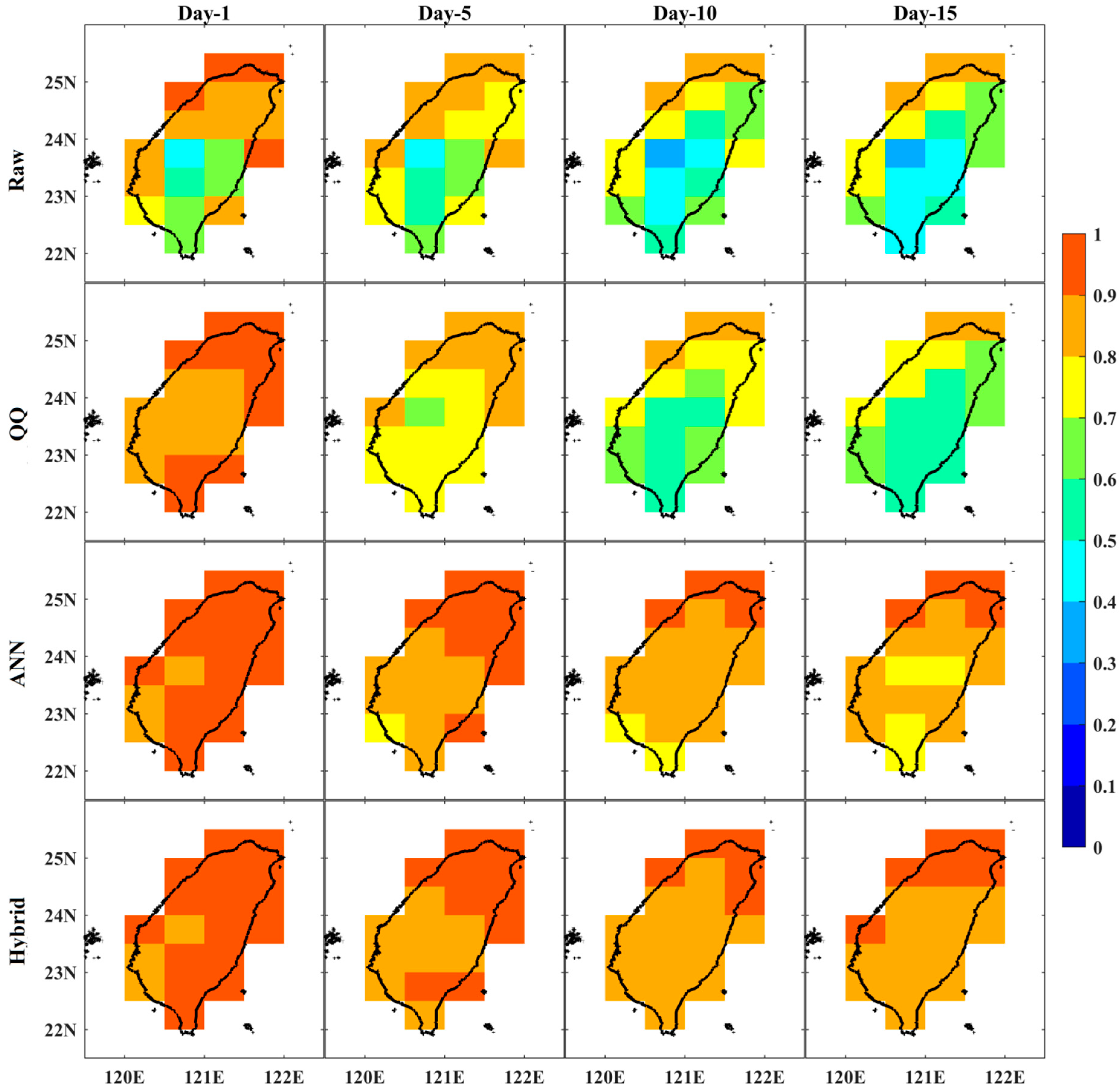
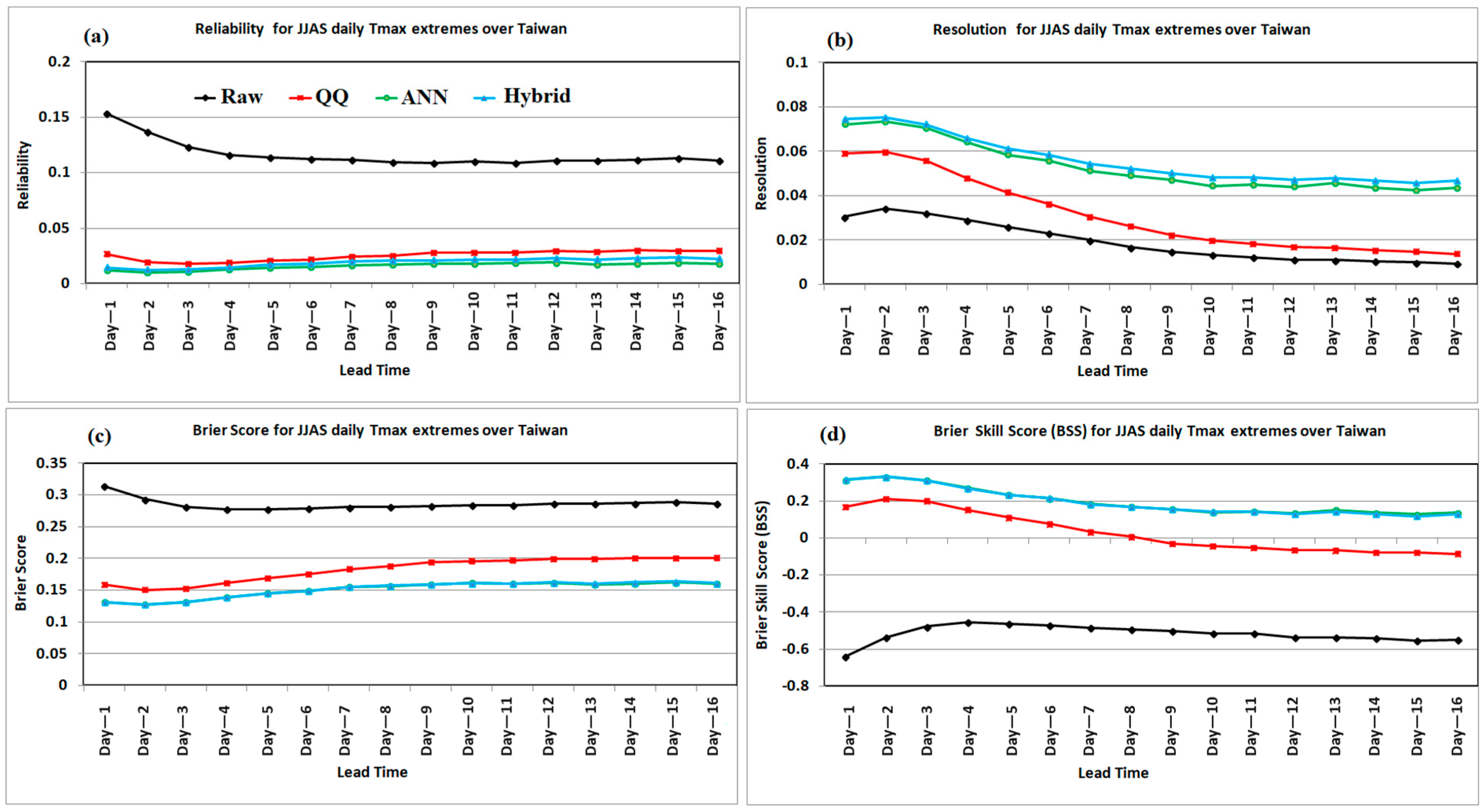
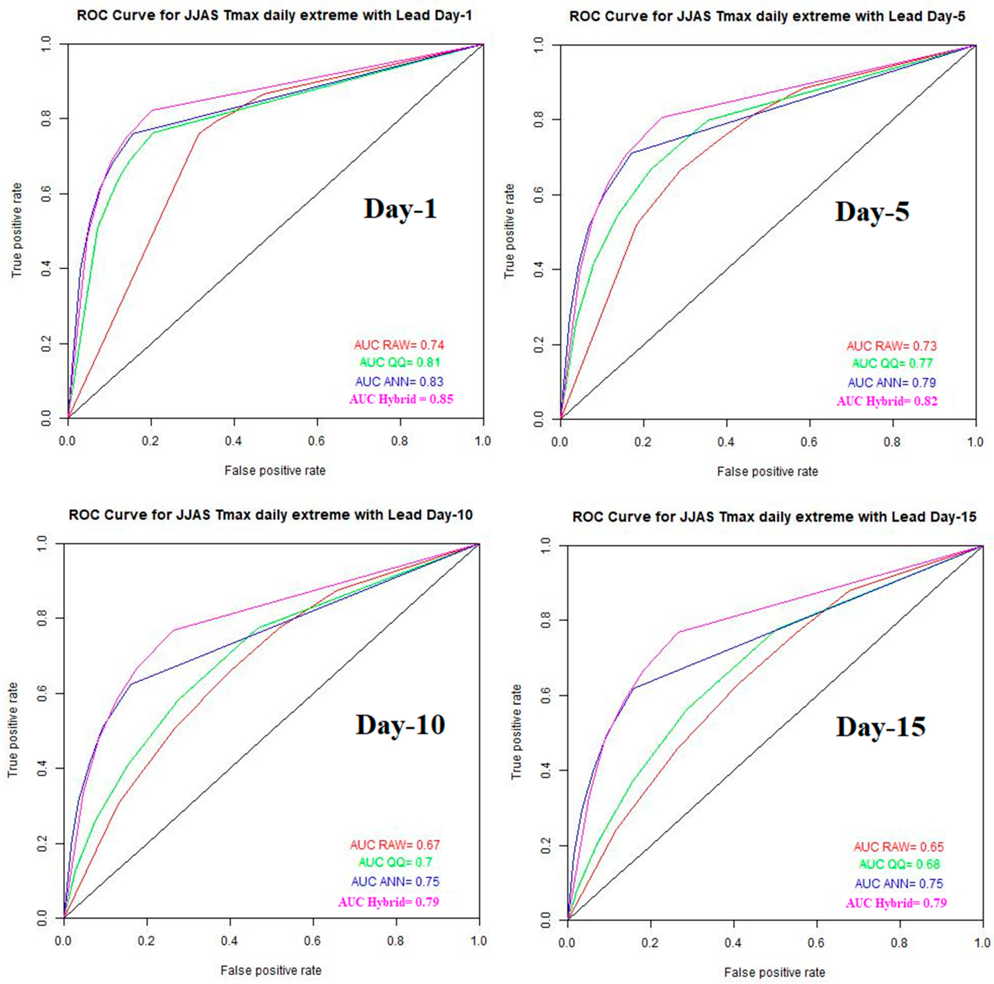
3.3. Probabilistic Prediction Skill Scores of Raw, QQ, ANN, and Hybrid Methods for Summer Daily Tmax Extremes

The uncertainty of summer Tmax extremes over Taiwan can be evaluated using metrics such as resolution, reliability, Brier score, Brier skill score, and ROC curves to assess the ensemble probabilistic forecast. The GEFSv12 probabilistic forecast of summer Tmax extreme days over Taiwan has a good reliability (<0.15) for all forecast lead times, as shown in Figure 11a. This was further improved by the application of three calibration methods (<0.05). The reliability of the forecast decreases with increasing lead time for Raw and all three calibration methods. However, the ANN and Hybrid methods showed the highest reliability, particularly a large improvement for longer lead time forecasts. The resolution of the GEFSv12 model for probabilistic forecasts of summer Tmax extreme days over Taiwan decreases with increasing forecast lead time, with higher resolution for shorter lead times (Figure 11b). All three calibration techniques significantly improved the resolution of the ensemble probabilistic forecast of summer Tmax extreme days over Taiwan for all forecast lead times. ANN and Hybrid methods showed the highest resolution. A significant improvement in the resolution of ANN and Hybrid methods has been noticed, especially for longer lead times. The Hybrid calibration method has a relatively better resolution than the ANN for all forecast lead times (Figure 11b). The Brier score (BS) is a metric used to measure the accuracy of binary predictions, where the result is either yes or no. The ideal score is 0. According to Figure 11c, the confidence of GEFSv12’s ensemble probabilistic forecasts of summer Tmax extreme days over Taiwan is low (BS > 0.25) for all forecast lead times. However, the calibration methods used were found to be highly effective in improving the accuracy (BS < 0.2) of these forecasts. Specifically, the ANN and Hybrid calibration methods showed higher accuracy than the QQ method. The Hybrid method of ensemble probabilistic forecasting of summer Tmax extreme days over Taiwan produces results similar to those of the ANN for all forecast lead times (Figure 11c). The GEFSv12 ensemble probabilistic forecasting of summer Tmax extreme days over Taiwan with a BSS of less than −0.4 was not as accurate as the climatological/random forecast for all forecast lead times. This was evident from the results shown in Figure 11d. However, the use of calibration methods such as QQ, ANN, and Hybrid methods improved the BSS remarkably for all forecast lead times. The QQ method was found to be the most accurate for up to one week lead time than the reference/climatological/random forecast. After the first week, the ensemble probabilistic forecasting of summer Tmax extreme days over Taiwan from QQ was not as accurate as expected as the random forecast. However, the ANN and Hybrid methods outperformed both the random/climatological and QQ forecasts for all forecast lead times (Figure 11d). The Hybrid method is more effective than ANN for predicting extreme summer Tmax days over Taiwan for all forecast lead times.
As a final diagnostic, we use the ROC curve to assess a model’s ability to distinguish between events and non-events. The ROC curve evaluates the forecast if a summer Tmax extreme day had occurred. It plots the true positive rate (correctly predicted Tmax extreme day) against the false positive rate (incorrectly predicted Tmax extreme day). We calculate the true positive rate and false positive rate for cumulative probabilities ranging from 0% to 100% in increments of 10%. A skillful forecasting model should have a higher true positive rate than a false positive rate, resulting in an ROC curve that curves towards the top-left corner of the plot. Conversely, a forecast system with no skill would be a straight line along the diagonal, indicating that the forecast is no better than a random guess. The AUC (Area Under the Curve) is a useful scalar measure for summarizing the performance of a model, with a score of 1 indicating the highest level of skill and a score of 0 indicating the lowest level of skill. The ROC curves for Raw, QQ, ANN, and Hybrid calibration methods for ensemble probabilistic forecasting of summer Tmax extreme days over Taiwan are all above the diagonal line for all forecast lead times, as shown in Figure 12.
Raw and all three calibration methods for ensemble probabilistic forecasting of summer Tmax extreme days over Taiwan have a satisfactory AUC skill score (>0.65) for all forecast lead times. However, it has been observed that the AUC skill decreases with increasing forecast lead times. The Hybrid calibration method yielded the highest AUC skill score (0.79–0.85), followed by ANN (0.75–0.83), QQ (0.68–0.81), and Raw (0.65–0.74). The performance analysis of three calibration methods revealed that they significantly improved the accuracy of GEFSv12 in forecasting extreme summer Tmax days in Taiwan. The Hybrid calibration method for ensemble probabilistic forecasting of summer Tmax extreme days on an extended-range time scale over Taiwan has been shown to be more effective than the QQ and ANN techniques.

4. Summary and Conclusions

The IPCC 2013 report highlighted an increase in global temperatures by 0.13 °C per decade over the past 50 years, a rate that is twice that of the previous century. Rising global temperatures significantly affect various sectors, including energy, aviation, and agriculture. The frequency and intensity of heat waves, particularly in Asia, have escalated. For example, in Taiwan, the air temperature rose by 1.4 °C between 1911 and 2005, which is double the increase recorded in the Northern Hemisphere. Research indicates a significant increase in respiratory and cardiovascular mortalities directly linked to temperature increases above certain thresholds. Current weather prediction systems face challenges forecasting extreme conditions 10 days to a month in advance due to complexities in tropical processes. Smaller regions like Taiwan require enhanced global models to accurately depict land–sea contrast and topography. Alongside model improvements, refining post-processing techniques is also imperative.
In September 2020, NOAA NCEP upgraded its Global Ensemble Forecast System to version 12 (GEFSv12) to improve the accuracy of sub-seasonal forecasts for meteorological and hydrological applications. This model was used to generate consistent reforecast products based on daily 00 UTC initial conditions for forecasts extended up to 16 days with five ensemble members for a period of 2000–2019, except every Wednesday when the forecasts were integrated up to 35 days with 11 members. The output of the model is subject to a high degree of uncertainty and is rarely used as-is. Therefore, post-processing techniques are used to reduce the uncertainty and improve the accuracy of the forecasts. In this study, a Hybrid calibration method combining Artificial Neural Network (ANN) and quantile–quantile mapping (QQ) techniques was applied to the GEFSv12 reforecasts to enhance the accuracy of summer daily Tmax and related Tmax extremes over Taiwan. The performance of the Hybrid technique was evaluated against ERA5 reanalysis and compared to the Raw, ANN, and QQ techniques using standard skill metrics for deterministic and ensemble probabilistic forecasts.
The GEFSv12 model was found to accurately replicate the spatial patterns of maximum temperature and its variability in Taiwan for all forecast lead times. However, it had a warm bias and overestimated the interannual variability (IAV) of Tmax in the southern and inland regions of Taiwan. The RMSE of the raw model and all three calibration methods increased with increasing forecast lead time. The Raw forecast for summer Tmax over Taiwan exhibited a high RMSE across all forecast lead times. However, all the calibration methods, such as QQ (0.8–1.2 °C), ANN (0.6–1 °C), and Hybrid (0.6–1 °C), notably reduced the RMSE for all forecast lead times. The QQ method yielded the highest RMSE compared to the ANN and Hybrid methods for all forecast lead times. The RMSE from the ANN and Hybrid methods were similar for all forecast lead times. Calibration techniques were effective in reducing the warm bias of ~0 °C in Taiwan during summer for all forecast lead times. The GEFSv12 model shows a strong correlation with summer daily Tmax over Taiwan, with a coefficient of more than 0.8 for Day-1 lead time forecasts. This correlation decreases with increasing forecast lead time, ranging from 0.8 to 0.4. No improvement was observed in the correlation coefficient when using the QQ method compared to the Raw products for all forecast lead times. However, the ANN and Hybrid calibration methods showed a significant improvement in the correlation coefficient for all forecast lead times, with the improvement being more pronounced for longer lead time forecasts. The IOA of GEFSv12 for predicting Taiwan’s Tmax shows a decrease from 0.8 to 0.6 as the forecast lead time increases, with higher values for shorter lead times. All calibration methods demonstrated a significant increase in the IOA of predicting daily summer Tmax over Taiwan for all forecast lead times. The ANN and Hybrid methods achieved scores of 0.88–0.92, while the QQ method had scores of 0.67–0.9. The Hybrid method yielded higher IOA values than the ANN for all forecast lead times.
The GEFSv12 model overestimated the number of Tmax extreme days over Taiwan, but this was reduced by the QQ, ANN, and Hybrid methods. The ANN model had the lowest number of heatwave days compared to the QQ and Hybrid approaches. The Hybrid method had the highest statistical categorical skill scores for all forecast lead times, outperforming the other two methods in terms of ETS, TS, SR, ACC, FAR, POD, and Frequency Bias. The prediction accuracy of Raw and all calibration methods for summer daily Tmax extremes over Taiwan is higher for Week-1, Week-2, and Week-1 to Week-2 forecasts than for day-to-day forecasts. The comparison of Week-1, 2, and 1 to 2 from Raw and all three calibration methods reveals that the prediction skill of Week-1 summer Tmax extreme days is superior to that of Week-2 and Week-1 to 2 when using Raw and all three calibration methods. The Hybrid method is more effective than the other two methods. The Hybrid method of forecasting extreme Tmax over Taiwan was found to be more effective than either QQ or ANN alone, based on the evaluation of probabilistic skill scores (reliability, resolution, Brier score, Brier skill score, and ROC curve). The Hybrid-calibrated GEFSv12 forecast can be beneficial in managing climate risk in Taiwan by providing extended-range forecasts of Tmax and associated extremes.

Author Contributions

Conceptualization, M.M.N., V.T. and Y.Z.; methodology, M.M.N. and Y.Z.; software, M.M.N.; validation, M.M.N., V.T. and Y.Z.; formal analysis, M.M.N.; investigation, M.M.N. and Y.Z.; resources, V.T.; data curation, M.M.N. and M.-S.C.; writing—original draft preparation, M.M.N.; writing—review and editing, V.T. and Y.Z.; visualization, M.M.N.; supervision, V.T. and Y.Z.; project administration, V.T.; funding acquisition, V.T. All authors have read and agreed to the published version of the manuscript.

Funding

This research received no external funding.

Institutional Review Board Statement

All the procedures performed in this study are in accordance with the ethical standards of the institute. The manuscript has not been submitted to more than one journal for simultaneous consideration. The manuscript has not been published elsewhere previously.

Informed Consent Statement

Not applicable.

Data Availability Statement

The maximum 2 m air temperature data for the period of 2000–2019 over Taiwan island have been obtained from ERA5 (https://cds.climate.copernicus.eu/cdsapp#!/dataset/reanalysis-era5-single-levels?tab=form (accessed on 1 June 2023)), while the GEFSv12 reforecast products for the same period have been retrieved from Amazon Web Services (AWS; https://noaa-gefs-retrospective.s3.amazonaws.com/index.html (accessed on 1 June 2023)).

Acknowledgments

This research was made possible through the NCEP Visiting Scientist Program, managed by the University Corporation for Atmospheric Research (UCAR) Cooperative Programs for the Advancement of Earth System Science (CPAESS). Binbin Zhou, Hong Guan, and Mary Hart are thanked for their careful reviews of the manuscript. The authors greatly appreciate the anonymous reviewers and the editor of the Atmosphere journal for their valuable suggestions and comments, which significantly improved the quality of the manuscript.

Conflicts of Interest

The authors declare no conflict of interest.

References

  1. IPCC. Climate Change 2013: The Physical Science Basis. Contribution of Working Group I to the Fifth Assessment Report of the Intergovernmental Panel on Climate Change; Stocker, T.F., Qin, D., Plattner, G.-K., Tignor, M., Allen, S.K., Boschung, J., Nauels, A., Xia, Y., Bex, V., Midgley, P.M., Eds.; Cambridge University Press: Cambridge, UK, 2013. [Google Scholar]
  2. Honda, Y.; Sugimoto, K.; Ono, M. Adaptation to Climate Change at Population Level in Japan. Epidemiology 2011, 22, S26. [Google Scholar] [CrossRef]
  3. Nageswararao, M.M.; Mohanty, U.C.; Prasad, S.K.; Osuri, K.K.; Ramakrishna, S.S.V.S. Performance evaluation of NCEP climate forecast system for the prediction of winter temperatures over India. Theor. Appl. Clim. 2016, 126, 437–451. [Google Scholar] [CrossRef]
  4. Nageswararao, M.M.; Sinha, P.; Mohanty, U.C.; Mishra, S. Occurrence of More Heat Waves Over the Central East Coast of India in the Recent Warming Era. Pure Appl. Geophys. 2020, 177, 1143–1155. [Google Scholar] [CrossRef]
  5. Karrevula, N.R.; Ramu, D.A.; Nageswararao, M.M.; Rao, A.S. Inter-annual variability of pre-monsoon surface air temperatures over India using the North American Multi-Model Ensemble models during the global warming era. Theor. Appl. Clim. 2023, 151, 133–151. [Google Scholar] [CrossRef]
  6. Rastogi, D.; Lehner, F.; Ashfaq, M. Revisiting Recent U.S. Heat Waves in a Warmer and More Humid Climate. Geophys. Res. Lett. 2020, 47, e2019GL086736. [Google Scholar] [CrossRef]
  7. Fischer, E.M.; Schär, C. Consistent geographical patterns of changes in high-impact European heatwaves. Nat. Geosci. 2010, 3, 398–403. [Google Scholar] [CrossRef]
  8. Meehl, G.A.; Tebaldi, C. More intense, more frequent, and longer lasting heat waves in the 21st century. Science 2004, 305, 994–997. [Google Scholar] [CrossRef]
  9. Smoyer-Tomic, K.E.; Kuhn, R.; Hudson, A. Heat Wave Hazards: An Overview of Heat Wave Impacts in Canada. Nat. Hazards 2003, 28, 465–486. [Google Scholar] [CrossRef]
  10. Wang, J.; Yan, Z.; Quan, X.-W.; Feng, J. Urban warming in the 2013 summer heat wave in eastern China. Clim. Dyn. 2017, 48, 3015–3033. [Google Scholar] [CrossRef]
  11. Nageswararao, M.M.; Zhu, Y.; Tallapragada, V.; Chen, M.-S. Prediction Skill of GEFSv12 in Depicting Monthly Rainfall and Associated Extreme Events over Taiwan during the Summer Monsoon. Weather Forecast. 2022, 37, 2239–2262. [Google Scholar] [CrossRef]
  12. Huang, R.H.; Chen, J.L.; Wang, L.; Lin, Z.D. Characteristics, processes, and causes of the spatio-temporal variabilities of the East Asian monsoon system. Adv. Atmos. Sci. 2012, 29, 910–942. [Google Scholar] [CrossRef]
  13. Lin, C.Y.; Chua, Y.J.; Sheng, Y.F.; Hsu, H.H.; Cheng, C.T.; Lin, Y.Y. Altitudinal and latitudinal dependence of future warming in Taiwan simulated by WRF nested with ECHAM5/MPIOM. Int. J. Clim. 2014, 35, 1800–1809. [Google Scholar] [CrossRef]
  14. IPCC. Intergovernmental Panel on Climate Change, Fourth Assesment Report: Climate Change 2007; IPPC: Geneva, Switzerland, 2007. [Google Scholar]
  15. Chung, J.-Y.; Honda, Y.; Hong, Y.-C.; Pan, X.-C.; Guo, Y.-L.; Kim, H. Ambient temperature and mortality: An international study in four capital cities of East Asia. Sci. Total. Environ. 2009, 408, 390–396. [Google Scholar] [CrossRef] [PubMed]
  16. Mariotti, A.; Ruti, P.M.; Rixen, M. Progress in subseasonal to seasonal prediction through a joint weather and climate community effort. Npj Clim. Atmos. Sci. 2018, 1, 4. [Google Scholar] [CrossRef]
  17. Li, S.; Robertson, A.W. Evaluation of Submonthly Precipitation Forecast Skill from Global Ensemble Prediction Systems. Mon. Weather Rev. 2015, 143, 2871–2889. [Google Scholar] [CrossRef]
  18. Vitart, F.; Ardilouze, C.; Bonet, A.; Brookshaw, A.; Chen, M.; Codorean, C.; Déqué, M.; Ferranti, L.; Fucile, E.; Fuentes, M.; et al. The sub-seasonal to seasonal prediction project (S2S) and the prediction of extreme events. Bull. Am. Meteorol. Soc. 2017, 98, 163–173. [Google Scholar] [CrossRef]
  19. Nageswararao, M.M.; Zhu, Y.; Tallapragada, V. Prediction Skill of GEFSv12 for Southwest Summer Monsoon Rainfall and Associated Extreme Rainfall Events on Extended Range Scale over India. Weather Forecast. 2022, 37, 1135–1156. [Google Scholar] [CrossRef]
  20. Kang, I.-S.; Jin, K.; Wang, B.; Lau, K.M.; Shukla, J.; Krishnamurthy, V.; Schubert, S.; Wailser, D.; Stern, W.; Kitoh, A.; et al. Intercomparison of the climatological variations of Asian summer monsoon precipitation simulated by 10 GCMs. Clim. Dyn. 2022, 19, 383–395. [Google Scholar] [CrossRef]
  21. Glahn, H.R.; Lowry, D.A. The use of model output statistics (MOS) in objective weather forecasting. J. Appl. Meteorol. 1972, 11, 1203. [Google Scholar] [CrossRef]
  22. Hamill, T.M.; Colucci, S.J. Evaluation of Eta–RSM Ensemble Probabilistic Precipitation Forecasts. Mon. Weather Rev. 1998, 126, 711–724. [Google Scholar] [CrossRef]
  23. Yagli, G.M.; Yang, D.; Srinivasan, D. Ensemble solar forecasting using data-driven models with probabilistic post-processing through GAMLSS. Sol. Energy 2020, 208, 612–622. [Google Scholar] [CrossRef]
  24. Li, M.; Wang, Q.; Robertson, D.E.; Bennett, J.C. Improved error modelling for streamflow forecasting at hourly time steps by splitting hydrographs into rising and falling limbs. J. Hydrol. 2017, 555, 586–599. [Google Scholar] [CrossRef]
  25. Vannitsem, S.; Wilks, D.S.; Messner, J.W. (Eds.) Chapter 3: Univariate ensemble forecasting. In Statistical Postprocessing of Ensemble Forecasts; Elsevier BV: Amsterdam, The Netherlands, 2018; ISBN 9780128123720. [Google Scholar]
  26. Ebert, E.E. Ability of a Poor Man’s Ensemble to Predict the Probability and Distribution of Precipitation. Mon. Weather Rev. 2001, 129, 2461–2480. [Google Scholar] [CrossRef]
  27. Hamill, T.M.; Whitaker, J.S. Probabilistic Quantitative Precipitation Forecasts Based on Reforecast Analogs: Theory and Application. Mon. Weather Rev. 2006, 134, 3209–3229. [Google Scholar] [CrossRef]
  28. Zhu, Y.; Luo, Y. Precipitation Calibration Based on the Frequency-Matching Method (FMM). Weather Forecast. 2015, 30, 1109–1124. [Google Scholar] [CrossRef]
  29. Guan, H.; Zhu, Y.; Sinsky, E.; Fu, B.; Li, W.; Zhou, X.; Xue, X.; Hou, D.; Peng, J.; Nageswararao, M.M.; et al. GEFSv12 Reforecast Dataset for Supporting Subseasonal and Hydrometeorological Applications. Mon. Weather Rev. 2022, 150, 647–665. [Google Scholar] [CrossRef]
  30. Zhao, T.; Bennett, J.C.; Wang, Q.J.; Schepen, A.; Wood, A.W.; Robertson, D.E.; Ramos, M.-H. How Suitable is Quantile Mapping For Postprocessing GCM Precipitation Forecasts? J. Clim. 2017, 30, 3185–3196. [Google Scholar] [CrossRef]
  31. Verkade, J.; Brown, J.; Reggiani, P.; Weerts, A. Post-processing ECMWF precipitation and temperature ensemble reforecasts for operational hydrologic forecasting at various spatial scales. J. Hydrol. 2013, 501, 73–91. [Google Scholar] [CrossRef]
  32. Wang, Q.; Shao, Y.; Song, Y.; Schepen, A.; Robertson, D.E.; Ryu, D.; Pappenberger, F. An evaluation of ECMWF SEAS5 seasonal climate forecasts for Australia using a new forecast calibration algorithm. Environ. Model. Softw. 2019, 122, 104550. [Google Scholar] [CrossRef]
  33. Zhou, X.; Zhu, Y.; Fu, B.; Hou, D.; Peng, J.; Luo, Y.; Li, W. The development of the Next NCEP Global Ensemble Forecast System. Science and Technology Infusion Climate Bulletin, NOAA’s National Weather Service. In Proceedings of the 43rd NOAA Annual Climate Diagnostics and Prediction Workshop (CDPW), Santa Barbara, CA, USA, 23–25 October 2019; pp. 159–163. [Google Scholar]
  34. Zhou, X.; Zhu, Y.; Hou, D.; Fu, B.; Li, W.; Guan, H.; Sinsky, E.; Kolczynski, W.; Xue, X.; Luo, Y.; et al. The Development of the NCEP Global Ensemble Forecast System Version 12. Weather Forecast. 2022, 37, 1069–1084. [Google Scholar] [CrossRef]
  35. Hamill, T.M.; Whitaker, J.S.; Shlyaeva, A.; Bates, G.; Fredrick, S.; Pegion, P.; Sinsky, E.; Zhu, Y.; Tallapragada, V.; Guan, H.; et al. The Reanalysis for the Global Ensemble Forecast System, Version 12. Mon. Weather Rev. 2022, 150, 59–79. [Google Scholar] [CrossRef]
  36. Harris, L.M.; Lin, S.-J. A Two-Way Nested Global-Regional Dynamical Core on the Cubed-Sphere Grid. Mon. Weather Rev. 2013, 141, 283–306. [Google Scholar] [CrossRef]
  37. Han, J.; Wang, W.; Kwon, Y.C.; Hong, S.-Y.; Tallapragada, V.; Yang, F. Updates in the NCEP GFS Cumulus Convection Schemes with Scale and Aerosol Awareness. Weather Forecast. 2017, 32, 2005–2017. [Google Scholar] [CrossRef]
  38. Han, J.-Y.; Hong, S.-Y.; Lim, K.-S.S.; Han, J. Sensitivity of a Cumulus Parameterization Scheme to Precipitation Production Representation and Its Impact on a Heavy Rain Event over Korea. Mon. Weather Rev. 2016, 144, 2125–2135. [Google Scholar] [CrossRef]
  39. Clough, S.; Shephard, M.; Mlawer, E.; Delamere, J.; Iacono, M.; Cady-Pereira, K.; Boukabara, S.; Brown, P. Atmospheric radiative transfer modeling: A summary of the AER codes. J. Quant. Spectrosc. Radiat. Transf. 2005, 91, 233–244. [Google Scholar] [CrossRef]
  40. Chun, H.-Y.; Baik, J.-J. Momentum Flux by Thermally Induced Internal Gravity Waves and Its Approximation for Large-Scale Models. J. Atmos. Sci. 1998, 55, 3299–3310. [Google Scholar] [CrossRef]
  41. Alpert, J.C.; Kanamitsu, M.; Caplan, P.M.; Sela, J.G.; White, G.H.; Kalnay, E. Mountain induced gravity wave drag parameterization in the NMC medium-range forecast model. In Proceedings of the Eighth Conference on Numerical Weather Prediction, Baltimore, MD, USA, 22–26 February 1988; American Meteorological Society: Boston, MA, USA, 1988; pp. 726–733. [Google Scholar]
  42. Zhu, Y.; Zhou, X.; Peña, M.; Li, W.; Melhauser, C.; Hou, D. Impact of Sea Surface Temperature Forcing on Weeks 3 and 4 Forecast Skill in the NCEP Global Ensemble Forecasting System. Weather Forecast. 2017, 32, 2159–2174. [Google Scholar] [CrossRef]
  43. Zhu, Y.; Zhou, X.; Li, W.; Hou, D.; Melhauser, C.; Sinsky, E.; Peña, M.; Fu, B.; Guan, H.; Kolczynski, W.; et al. Toward the Improvement of Subseasonal Prediction in the National Centers for Environmental Prediction Global Ensemble Forecast System. J. Geophys. Res. Atmos. 2018, 123, 6732–6745. [Google Scholar] [CrossRef]
  44. Li, W.; Zhu, Y.; Zhou, X.; Hou, D.; Sinsky, E.; Melhauser, C.; Peña, M.; Guan, H.; Wobus, R. Evaluating the MJO prediction skill from different configurations of NCEP GEFS extended forecast. Clim. Dyn. 2019, 52, 4923–4936. [Google Scholar] [CrossRef]
  45. Shutts, G. A kinetic energy backscatter algorithm for use in ensemble prediction systems. Q. J. R. Meteorol. Soc. 2005, 131, 3079–3102. [Google Scholar] [CrossRef]
  46. Shutts, G.; Palmer, T.N. The use of high-resolution numerical simulations of tropical circulation to calibrate stochastic physics schemes. In Proceedings of the ECMWF/CLIVAR Workshop on Simulation and Prediction of Intra-Seasonal Variability with Emphasis on the MJO, Reading, UK, 3–6 November 2004; pp. 83–102. Available online: https://www.ecmwf.int/node/12212 (accessed on 10 June 2023).
  47. Buizza, R.; Milleer, M.; Palmer, T.N. Stochastic representation of model uncertainties in the ECMWF ensemble prediction system. Q. J. R. Meteorol. Soc. 1999, 125, 2887–2908. [Google Scholar] [CrossRef]
  48. Palmer, T.N.; Buizza, R.; Doblas-Reyes, F.; Jung, T.; Leutbecher, M.; Shutts, G.J.; Steinheimer, M.; Weisheimer, A. Stochastic parametrization and model uncertainty. ECMWF Tech. Memo. 2009, 598, 42. [Google Scholar]
  49. Hersbach, H.; Bell, B.; Berrisford, P.; Biavati, G.; Horányi, A.; Muñoz Sabater, J.; Nicolas, J.; Peubey, C.; Radu, R.; Rozum, I.; et al. ERA5 Hourly Data on Single Levels from 1959 to Present. Copernicus Climate Change Service (C3S) Climate Data Store (CDS). 2018. Available online: https://doi.org/10.24381/cds.adbb2d47 (accessed on 1 June 2023).
  50. Lee, C.-T.; Wang, S.-Y.S.; Lo, T.-T. A Revised Meiyu-Season Onset Index for Taiwan Based on ERA5. Atmosphere 2022, 13, 1762. [Google Scholar] [CrossRef]
  51. Tarek, M.; Brissette, F.P.; Arsenault, R. Evaluation of the ERA5 reanalysis as a potential reference dataset for hydrological modelling over North America. Hydrol. Earth Syst. Sci. 2020, 24, 2527–2544. [Google Scholar] [CrossRef]
  52. Velikou, K.; Lazoglou, G.; Tolika, K.; Anagnostopoulou, C. Reliability of the ERA5 in Replicating Mean and Extreme Temperatures across Europe. Water 2022, 14, 543. [Google Scholar] [CrossRef]
  53. McNicholl, B.; Lee, Y.H.; Campbell, A.G.; Dev, S. Evaluating the reliability of air temperature from ERA5 reanalysis data. IEEE Geosci. Remote Sens. Lett. 2021, 19, 1004505. [Google Scholar] [CrossRef]
  54. Piani, C.; Haerter, J.O.; Coppola, E. Statistical bias correction for daily precipitation in regional climate models over Europe. Theor. Appl. Clim. 2010, 99, 187–192. [Google Scholar] [CrossRef]
  55. Saxena, A.; Verma, N.; Tripathi, K.C. A review study of weather forecasting using artificial neural network approach. Int. J. Eng. Res. Technol. 2013, 2, 2029–2035. [Google Scholar]
  56. Al-Matarneh, L.; Sheta, A.; Bani-Ahmad, S.; Alshaer, J.; Al-Oqily, I. Development of Temperature-based Weather Forecasting Models Using Neural Networks and Fuzzy Logic. Int. J. Multimedia Ubiquitous Eng. 2014, 9, 343–366. [Google Scholar] [CrossRef]
  57. Feng, J.; Lu, S. Performance Analysis of Various Activation Functions in Artificial Neural Networks. J. Phys. Conf. Ser. 2019, 1237, 022030. [Google Scholar] [CrossRef]
  58. Abbot, J.; Marohasy, J. Input selection and optimisation for monthly rainfall forecasting in Queensland, Australia, using artificial neural networks. Atmos. Res. 2014, 138, 166–178. [Google Scholar] [CrossRef]
  59. Yilmaz, A.; Imteaz, M.; Jenkins, G. Catchment flow estimation using Artificial Neural Networks in the mountainous Euphrates Basin. J. Hydrol. 2011, 410, 134–140. [Google Scholar] [CrossRef]
  60. Ahmad, R.; Lazin, N.M.; Samsuri, S.F.M. Neural network modeling and identification of naturally ventilated tropical greenhouse climates. Wseas Trans. Syst. Control 2014, 9, 445–453. [Google Scholar]
  61. Mcculloch, W.S.; Pitts, W.H. A logical calculus of the ideas immanent in nervous activity. Bull. Math. Biophys. 1943, 5, 115–133. [Google Scholar] [CrossRef]
  62. Fausett, L. Fundamentals of Neural Network; Prentice Hall: Hoboken, NJ, USA, 1994. [Google Scholar]
  63. Singh, G.; Panda, R.K. Daily sediment yield modeling with artificial neural network using 10-fold cross validation method: A small agricultural watershed, Kapgari, India. Int. J. Earth Sci. Eng. 2011, 4, 443–450. [Google Scholar]
  64. Singh, G.; Panda, R.K. Bootstrap-based artificial neural network analysis for estimation of daily sediment yield from a small agricultural watershed. Int. J. Hydrol. Sci. Technol. 2015, 5, 333. [Google Scholar] [CrossRef]
  65. Hecht-Nielsen, R. Kolmogorov’s mapping neural network existence theorem. In Proceedings of the International Conference on Neural Networks, San Diego, CA, USA, 1 October 1987; IEEE Press: New York, NY, USA, 1987; Volume 3, pp. 11–14. [Google Scholar]
  66. Nair, A.; Singh, G.; Mohanty, U.C. Prediction of Monthly Summer Monsoon Rainfall Using Global Climate Models Through Artificial Neural Network Technique. Pure Appl. Geophys. 2018, 175, 403–419. [Google Scholar] [CrossRef]
  67. Johnstone, C.; Sulungu, E.D. Application of neural network in prediction of temperature: A review. Neural Comput. Appl. 2021, 33, 11487–11498. [Google Scholar] [CrossRef]
  68. Roebber, P.J. Visualizing Multiple Measures of Forecast Quality. Weather Forecast. 2009, 24, 601–608. [Google Scholar] [CrossRef]
  69. Brier, G.W. Verification of forecasts expressed in terms of probability. Mon. Weather Rev. 1950, 78, 1–3. [Google Scholar] [CrossRef]
  70. Toth, Z.; Talagrand, O.; Candille, G.; Zhu, Y. Probability and ensemble forecasts. Forecast Verification: A Practitioner’s Guide in Atmospheric Science; Jolliffe, I.T., Stephenson, D.B., Eds.; Wiley: Hoboken, NJ, USA, 2003; pp. 137–163. [Google Scholar]
  71. Weijs, S.V.; van Nooijen, R.; van de Giesen, N. Kullback–Leibler Divergence as a Forecast Skill Score with Classic Reliability–Resolution–Uncertainty Decomposition. Mon. Weather Rev. 2010, 138, 3387–3399. [Google Scholar] [CrossRef]
  72. Marzban, C. The ROC Curve and the Area under It as Performance Measures. Weather Forecast. 2004, 19, 1106–1114. [Google Scholar] [CrossRef]
Figure 1. (a) Schematic flow chart of methodology and (b) Artificial Neural Network architecture used in this study.
Atmosphere 14 01620 g001
Figure 2. Climatological mean of summer (JJAS) surface air maximum temperature (Tmax) over Taiwan from ERA5, Raw, QQ, ANN, and Hybrid methods with Day-1, 5, 10, and 15 forecast lead times for the period of 2000–2019.
Atmosphere 14 01620 g002
Figure 3. Interannual variability of summer (JJAS) surface air maximum temperature (Tmax) over Taiwan from ERA5, Raw, QQ, ANN, and Hybrid methods with Day-1, 5, 10, and 15 forecast lead times for the period of 2000–2019.
Atmosphere 14 01620 g003
Figure 4. RMSE (°C) of Raw, QQ, ANN, and Hybrid methods with Day-1, 5, 10, and 15 forecast lead times against ERA5 in depicting summer (JJAS) surface air maximum temperature (Tmax) over Taiwan for the period of 2000–2019.
Atmosphere 14 01620 g004
Figure 5. Index of Agreement of Raw, QQ, ANN, and Hybrid methods with Day-1, 5, 10, and 15 forecast lead times against ERA5 in depicting summer (JJAS) surface air maximum temperature (Tmax) over Taiwan for the period of 2000–2019.
Atmosphere 14 01620 g005
Figure 6. (a) Root Mean Squared Error in °C, (b) mean bias in °C, (c) correlation coefficient, and (d) Index of Agreement of Raw, QQ, ANN, and Hybrid methods against ERA5 in depicting Summer daily Tmax over Taiwan for Day-1 to 16 lead time forecasts for the period of 2000–2019.
Atmosphere 14 01620 g006
Figure 7. The PDF of summer (JJAS) daily Tmax over Taiwan from ERA5 (black dotted lines), Raw (blue dotted lines), QQ (magenta dotted lines), ANN (cyan dotted lines), and Hybrid methods (Red dotted lines) for Day-1, 5, 10, and 15 forecast lead times for the reforecast period of 2000–2019.
Atmosphere 14 01620 g007
Figure 8. The Equitable Threat Score (ETS) of Raw, QQ, ANN, and Hybrid methods in depicting JJAS daily Tmax extremes over Taiwan against ERA5 with Day-1, 5, 10, and 15 forecast lead times for the period of 2000–2019.
Atmosphere 14 01620 g008
Figure 9. The Equitable Threat Score (ETS) of Raw, QQ, ANN, and Hybrid methods in depicting JJAS daily Tmax extremes over Taiwan against ERA5 for Week-1, 2, and 1 to 2 forecasts for the period of 2000–2019.
Atmosphere 14 01620 g009
Figure 10. Performance diagram illustrating the SR, POD, Frequency Bias, and TS statistical categorical skill scores of Raw, QQ, ANN, and Hybrid methods against ERA5 for JJAS daily Tmax extremes over Taiwan on (a) a daily scale with Day-1 to 16, and (b) weekly scale for Week-1, 2, and 1 to 2 for the period of 2000–2019 is presented, with solid and dashed lines representing TS and Frequency Bias scores, respectively.
Atmosphere 14 01620 g010
Figure 11. (a) Reliability, (b) resolution, (c) Brier score, and (d) Brier skill score of Raw, QQ, ANN, and Hybrid methods against ERA5 for summer daily Tmax extremes ensemble probabilistic forecast over Taiwan with Day-1 to 16 forecast lead times for the period of 2000–2019.
Atmosphere 14 01620 g011
Figure 12. Receiver operating characteristic (ROC) curve and area under the ROC curve of Raw, QQ, ANN, and Hybrid methods against ERA5 for summer extreme daily Tmax ensemble probabilistic forecast over Taiwan with Day-1, 5, 10, and 15 forecast lead times for the period of 2000–2019.
Atmosphere 14 01620 g012
Table 1. The following are considered to develop a simple ANN model to improve the GEFSv12 prediction skill in depicting summer daily Tmax and associate Tmax extremes over Taiwan.
No. of Hidden Layers: 1
No. of nodes/neurons in the hidden layer 7
Neural Network used Feed-forward network
Neural Network processing functionsMap matrix row minimum and maximum values to [−1, 1]
Data divided function 70% data for training and 30% data for validation
Learning rate 0.001
Max number of iterations/epochs used 1000
Error tolerance for stopping criterion 1 × 10⁻¹⁴
Training function used Supervised weight/bias training function with sequential order weight/bias training (trains)
Neural Network performance functions used Mean squared error performance function
Disclaimer/Publisher’s Note: The statements, opinions and data contained in all publications are solely those of the individual author(s) and contributor(s) and not of MDPI and/or the editor(s). MDPI and/or the editor(s) disclaim responsibility for any injury to people or property resulting from any ideas, methods, instructions or products referred to in the content.

