Harmonisation in Atmospheric Dispersion Modelling Approaches to Assess Toxic Consequences in the Neighbourhood of Industrial Facilities ^†

Abstract

In the land use planning framework in the neighbourhood of industrial facilities, the current approach to predicting the consequences of massive toxic gas releases is generally based on Gaussian or integral models. For many years, CFD models have been more and more used in this context, in accordance with the development of high-performance computing (HPC). The present paper focuses on harmonising input data for atmospheric transport and dispersion (AT&D) modelling between the widely used approaches. First, a synthesis of the practice’s harmonisation for atmospheric dispersion modelling within the framework of risk assessment is presented. Then, these practices are applied to a large-scale INERIS ammonia experimental release. For illustration purposes, the impact of the proposed harmonisation will be evaluated using different approaches: the SLAB model, the FDS model, and the Code_Saturne model. The two main focuses of this paper are the adaptation of the source term dealing with a massive release and the wind flow modelling performance using an experimental signal for CFD model inflow. Finally, comparisons between the modelling and experimental results enable checking the consistency of these approaches and reinforce the importance of the input data harmonisation for each AT&D modelling approach.

1. Introduction

1.1. Toxic Gas Atmospheric Dispersion Accidents

Several major accidents occurred in the last few decades due to the atmospheric release of dangerous substances. While the most known one is probably the Seveso in 1976 accident [1] with a large release of dioxins since its name was given to the European regulation, others like Bhopal in 1984 [2] with a massive release of methyl isocyanate, the massive release of carbon dioxide in Nyos, Cameroun in 1986 [3] or, more recently in 2022, a large ammonia release in Donaldsonville in the USA [4]. The number of such accidents is important, and being able to predict consequences is a huge challenge for protecting citizens.

Considering a general point of view in terms of citizens’ protection against industrial hazards, following the huge explosion that occurred in Toulouse, France, at the AZF factory [5], causing 31 deaths and thousands (~2500) of injured people on 21 September 2001, a dedicated regulation was built. Two years after this major industrial accident, a new regulation was introduced on 30 July 2003, which described both the prevention and repair of the damage caused by industrial and natural disasters. This regulation was the beginning of a general change of mind for environmental consequences evaluations; then regulations were made considerably tighter, and the entire approach towards risk assessment changed [5] in France. The Technological Risk Prevention Plan (“PPRT” in French, standing for Plan de Prévention des Risques Technologiques) is the new legislation tool aiming to protect people by acting on the existing urbanisation and by controlling future land-use planning in the vicinity of the existing Seveso establishments. The initial phase of PPRT development involves identifying potential scenarios, a crucial step in the multifactorial process. If a scenario is not proven to be physically impossible, it undergoes analysis to predict the potential outcomes of associated hazardous events. Subsequently, the analysis is followed by the prediction of the impact zone, encompassing the thermal, overpressure, and toxic effects generated by these dangerous phenomena. Computational tools are indispensable in this predictive process, where atmospheric dispersion models play a major role in estimating distances resulting from the release of toxic or flammable substances.

Various atmospheric modelling techniques are used in the framework of land use planning, encompassing a wide array of natures and complexities. In regulatory studies involving accidental releases of toxic or flammable materials into the atmosphere, significant disparities in computed distances can arise, leading to substantial differences in affected areas. These discrepancies are noticeable both among computational fluid dynamics (CFD) models and traditional methods like Gaussian or shallow layer approach models. There are numerous reasons behind these disparities, stemming from various sources, and they underscore the clear necessity for harmonisation. In the paper, the term “harmonisation” is employed to describe the process of constructing and employing AT&D models. This harmonisation is essential to guarantee that, regardless of the specific model employed within its designated scope, the results remain highly comparable. Among these disparities, three primary categories can be distinguished: those attributed to the model itself, those linked to the input data utilised, and those arising from user choices.

The aim of the harmonisation process is threefold:

• To offer direction during model development, ensuring consistent representation of physical phenomena, especially concerning the relationship between atmospheric turbulence and the diffusion coefficient for pollutants.
• To offer guidance on constructing input data for the model, including factors like the atmospheric wind and turbulence profile, the appropriate roughness value, and the specification of the source term within the AT&D model.
• To provide users with guidance that constrains potential individual choices, particularly concerning numerical parameters or mesh settings.

As atmospheric dispersion modelling continues to evolve as a research area over time, it becomes evident that certain decisions must be made. These decisions should be of a generic nature, guided by harmonisation principles, rather than being tailored individually for each study.

1.2. Context of AT&D Model Uses

As discussed in the previous paragraph, toxic or flammable releases can occur on several installations. AT&D model capabilities should be considered from several points of view to meet the objective of citizen protection.

The most obvious one is the capability to predict the worst-case situation in the land use planning context. In such an application, all potential scenarios identified during the risk analysis should be modelled, crossing the potential release situations with the riskiest atmospheric conditions. The typical result of such an application would be the distances reached by the corresponding thresholds for human beings.

A second application of the AT&D model consists of supporting firefighters in emergency situations by providing information on the potential concentration in the release surrounding. This information is then used either for firefighters’ protection choices or to inform the authorities about the required evacuation, as during the above-mentioned Donaldsonville, where a school should be evacuated. Having some relevant information about cloud behaviour in quite real-time is, in such a situation, highly valuable.

Finally, the AT&D model should be used to provide more detailed information on a specific case after the emergency phase by detailed modelling of the cloud behaviour or with a research point of view to improve capabilities for the two previous fields of use of such models [6].

It is clear that not the same approach can be used for those different situations since the accident details knowledge differs in-between. In emergency situations, typically, in most cases, the source term is just an approximation; during land use planning studies, the source term is a theoretical situation and; in post-accident or research studies, hopefully, the source term is better known. The situation is the same for the wind, which is known in a different manner for those different situations.

The AT&D model’s applicability is delineated through six key aspects: scenarios involving release or loss of containment (such as line rupture, catastrophic rupture, or vessel burst), the specific chemical products involved, hazardous substances or materials, environmental factors, geometry (factors influencing hazardous phenomena, not target definitions), analysis of hazardous effects and consequences, and the context of use—encompassing risk assessment regulatory studies, emergency situation technical support, and evaluation of damage to human health, life, environment, or infrastructure.

1.3. Objectives of the Study

The main objective of the present paper consists of breaking down the most common practices in AT&D modelling for accidental releases of toxic or flammable gas and putting forward what differences can result from this to provide some thinking about the harmonisation of practices between models. From the authors’ perspective, this subject is very rarely addressed in the scientific literature. This work represents a new approach to thinking about and illustrating data harmonisation for models.

The harmonisation process ensures that the mathematical and theoretical representation of physical phenomena remains consistent, regardless of the level of simplification used by the model. Additionally, harmonisation implies that the input data used for modelling are sufficiently well-defined to eliminate any need for interpretation during use.

This paper is structured as follows: In Section 2, an overview is provided of the primary practices in AT&D models for an accidental release, ranging from the simplest models to the most advanced ones. This section also presents descriptions of common models and their utilisation, with a specific focus on existing harmonisation methods and the introduction of new approaches aimed at enhancing harmonisation. In Section 3, the focus shifts to the application of AT&D models to a massive release across various model types. The primary objective of this section is to emphasise the significance of harmonising each aspect when utilising AT&D models. This section is then not directly focused on the application of harmonisation practices, since those practices are most relevant for prediction cases within the regulatory context. Instead, Section 3 illustrates how each parameter can significantly impact the results, underscoring the importance of harmonising these practices.

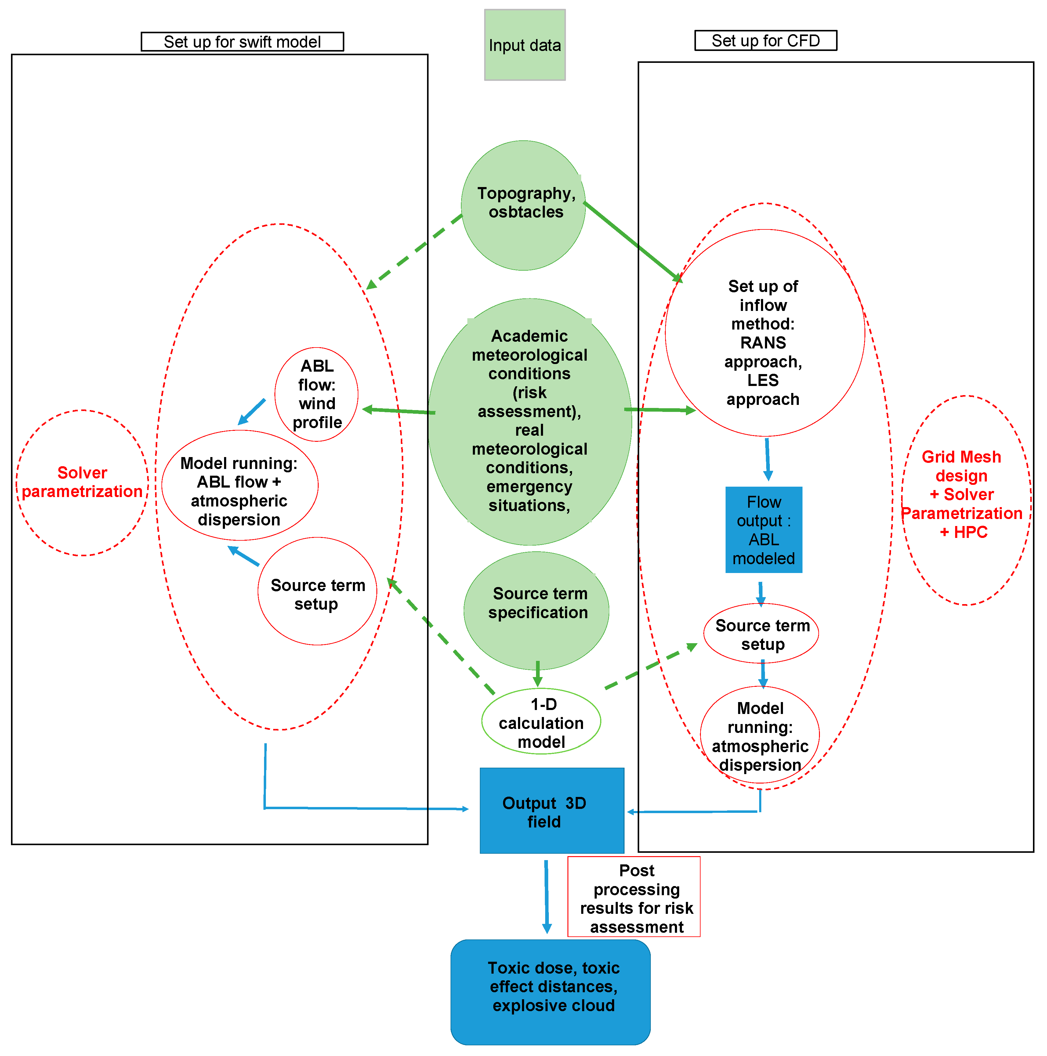
2. Main Steps of AT&D Modelling

The atmospheric dispersion computational models currently used are characterized by a large variety of nature and complexity. For the same analysed hazardous phenomena and physical characteristics, discrepancies appeared in computed distances or impacted zones between models. To provide a better understanding of the origin of these discrepancies, it is important to consider the main physical parameters and the way they are introduced into the different types of models, which will be the objective of the next sections of the chapter.

It is evident that the manner in which the models deal with physical parameters introduced differences before starting the simulation, as typically:

• the representation of the velocity and turbulence profile,
• the description of the emission source term,
• the differences in terms of physical phenomena considered in the model.

A diagram showing the main steps of AT&D modelling within the context of risk assessment is presented in Figure 1. This figure shows the most important topic to be considered in a harmonisation process, with the three points of view mentioned in Section 1.2, the model, left and right on the figure; input data, in green in the centre; and the user, who will run the model and make the choices. In the subsequent section of this chapter and in the following chapter, each element depicted in the figure will be comprehensively explained, outlining its potential impact on dispersion outcomes.

2.1. Background about Theoretical Approaches

A major issue for risk assessments is the harmonisation of input data for atmospheric modelling between widely used approaches, from simple gaussian or integral models to more complex ones such as CFD (RANS or LES) approaches, whose use is continuously increasing due to the easier use of high-performance computing. To the best of the authors’ knowledge, other approaches exist but are not yet widely used [7] at the microscale scale.

2.1.1. Gaussian Models

The simplest and probably the most used approaches are Gaussian models. Such models are rigorously restricted to neutral gas dispersion for releases that do not affect the atmospheric flow, such as low-momentum releases; this means that the released gas should have a density close to the air one or have been diluted enough. Such an approach assumes that atmospheric turbulence is the key parameter for gas dispersion that enables assuming a Gaussian-distributed gas concentration following the orthogonal directions of the flow [8]. Characteristics of atmospheric turbulence are then introduced through the standard deviation coefficients, σ, in the concentration equation. Among these, two main Gaussian approaches could be distinguished: the first series is designed for free field dispersion, and the second one includes analytical corrections to take into account obstacles [9]. A typical equation of the gas concentration, C, in space (x, y, z) and time, t, evolution can be written for a local and instantaneous release as follows:

$$\begin{gathered} C(x,y,z,t)=\frac{M}{(2\pi {)}^{\raisebox{1ex}{$3$}\!\left/ \!\raisebox{-1ex}{$2$}\right.}{\sigma }_x{\sigma }_y{\sigma }_z}\mathit{exp}\left(-\frac{(x-x_0-ut{)}^2}{2{\sigma }_x^2}\right. \\ \hspace{1em}\hspace{1em}\hspace{1em}\hspace{1em}\hspace{1em}\hspace{1em}\hspace{1em}\hspace{1em}\hspace{1em}\hspace{1em}\hspace{1em}\hspace{1em}\left.-\frac{(y-y_0{)}^2}{2{\sigma }_y^2}\right)\left[\mathit{exp}\left(\frac{(z-z_0{)}^2}{2{\sigma }_z^2}\right)+\alpha \hspace{0.33em}\mathit{exp}\left(\frac{(z+z_0{)}^2}{2{\sigma }_z^2}\right)\right] \end{gathered}$$

(1)

with M the discharge product (kg), u the mean wind speed (m/s), t time since the emission of the product, (x₀, y₀, z₀) the discharge location, and α a reflection coefficient on the ground. The standard deviation coefficients σ_x, σ_y, σ_z of the Gaussian distribution of the quantity of gas M in relation to its position at the instant t (m) are then based on experimental data, and several available sets in the literature are those proposed by [10,11,12].

2.1.2. Integral Models

When the discharge is such that it disturbs the atmospheric flow of air, it is inappropriate to use a Gaussian model, at least in the vicinity of this release. Physical mechanisms not considered by Gaussian models must be considered, such as the effects of dynamic turbulence. These concerns typically discharge with a high emission velocity, such as a jet; the effects of gravity for heavy gas discharges; and the floating effects for light gas discharges. The use of an integral model allows these mechanisms to be represented, and it explains their wide use. This type of model is based on simplified fluid mechanics equations set to provide a quick solution. The scalar conservation is assured by the integration into the volume delimited by the surface of the cloud; from this comes the “integral approach”. In addition, these models include, in most cases, a calculation module enabling the discharge source term to be determined according to the product’s storage conditions and the type of discharge (full bore-rupture tank rupture, pool evaporation, etc.) [13]. As soon as the release becomes passive, i.e., diluted enough and with low enough velocity, integral tools transition to a Gaussian model.

2.1.3. Shallow Layer Models

A specific family of integral-like models was developed to deal with heavier-than-air gas dispersion. Such models are based on one-dimensional equations of momentum, conservation of mass, species, and energy, and the equation of state resolution. It can handle release scenarios that are instantaneous, continuous, or with a finite duration, including ground-level and horizontal or vertical elevated jets, liquid pool evaporation, and instantaneous volume sources for the specific case of heavier than air gases, since this enables simplifying the equation set resolution. One of the most known shallow layer models is SLAB [14].

2.1.4. CFD Modelling

CFD (computational fluid dynamics) approaches consist of solving the full set of Navier-Stokes equations after having discretized the computational domains in cells. During a dispersion process, the key physical phenomenon that governs the gas mixture is turbulence. Solving the turbulence is the heart of those CFD models, and two main approaches can be used in that way: RANS (Reynolds Average Navier Stokes) [15] or LES (Large Eddy Simulation) [16] approaches for industrial application; DNS (Direct Numerical Simulation) is not realistic for such a large domain. One of the main differences between RANS and LES is the isotropic hypothesis for the turbulence used in most of the RANS approaches, while in LES models, only the modelled small scales are assumed to be isotropic; the solved scales, the higher ones, are not, meaning that the turbulence anisotropy could be solved [17,18]. Having in mind that atmospheric turbulence is strongly anisotropic, this is of primary importance. Another way to keep the anisotropic properties in the model is to use R_ij models [19].

Obviously, choosing the turbulent model implies considering the main physical parameters to be considered in it. An important aspect of atmospheric turbulence is the important relationship between the thermal gradient and the turbulence that leads to the distinction between:

• the neutral atmosphere, where the thermal gradient corresponds to the adiabatic gradient;
• the stable atmosphere, where the gradient is lower than the adiabatic one;
• the unstable atmosphere, where the gradient is higher than the adiabatic one.

Such a gradient would induce some convective displacement and, of course, influence the turbulence, which means that the thermal gradient influence should be considered in the turbulence model. Once more, natively in the LES approach, the turbulence anisotropy [20] and the density effect on the turbulence are included in the equations since they affect, more specifically, larger scales. On the other hand, in the RANS approach, an additional term should be added to the transport equation to introduce the density gradient influence on the turbulence. For such a specific application of k-ε models, ref. [21] proposed a specific set of constants together with an additional term in the k equation:

$$\mathrm{G}=\mathsf{\beta }\overline{\mathrm{w}\mathrm{\prime }.{\mathsf{\theta }}_{\mathrm{v}}\mathrm{\prime }}$$

(2)

where β expresses the floatability, β = g/θ_v, ${\theta }_{\mathrm{v}}\mathrm{\prime }$ is the fluctuation of the potential temperature, and w’ is the fluctuation of the vertical velocity component.

An important constraint of the LES approach, however, is the mesh criteria. Based on the fundamental principle of the LES approach, the resolved part of the turbulent should be important enough [17], with a minimum criterion that consists of a characteristic cutting scale in the inertial zone of the turbulent spectrum [22]. Since the same turbulent intensity can correspond to different turbulent spectrums, producing a reference method to build a representation of atmospheric turbulence from an LES point of view would be a great improvement.

Based on this state of the art, some recommendations should be proposed towards harmonisation of CFD practices, including:

• The turbulence model should consider the influence of the thermal gradient on the turbulence generation of suppression.
• The atmospheric turbulence anisotropy should be considered as a target when developing atmospheric dispersion models.
• Develop LES harmonised practices to build the input turbulence.

2.1.5. Harmonisation between Model Input Data

The objective of harmonisation between AT&D models is to achieve input data for each model, considering their respective domains of use. Some simplifications describing ABL, particularly in the regulatory context, are sometimes necessary, such as the stationary nature of ABL over the modelling period. Indeed, as defined by Stull [23], the atmospheric boundary layer is the part of the troposphere directly influenced by the presence of the Earth’s surface, such that it responds to surface forcing on time scales of the order of an hour. Starting from the hypothesis of stationary, it is necessary to make a choice between the vertical speed gradient and the vertical temperature gradient. These gradients are mainly due to the effects of air friction on the ground and heat exchanges between the ground and the atmosphere. These exchanges vary with the diurnal cycle, weather conditions, and the nature of the soil. At the end, the harmonisation of meteorological data pre-process means focusing on fundamental values describing ABL, such as Monin-Obukhov Lenght (LMO), friction velocity u*, wind speed (m/s) at an altitude reference, roughness, and the turbulent sensible heat flux. Meteorological profile construction will be given in detail in the next section.

2.2. From Meteorological Conditions to AT&Model Flow Input Data

Depending on the context, the nature and completeness of the flow data are fundamentally different. The mean wind at a reference altitude and information about atmospheric turbulence stability seem to be the minimal set of data to characterise the flow. One commonly employed method for characterising atmospheric turbulence stability is the turbulence classification scheme developed by Pasquill [12]. This system divides atmospheric turbulence into six stability classes labelled A, B, C, D, E, and F. Class A represents highly unstable conditions, while class F indicates moderately stable scenarios. In the context of an emergency, directly observed data by first responders or extraction for a meteorologically corrected forecast [24] can be scarce. Measured mean wind at a reference altitude and observation in situ, such as daytime insolation or cloudiness during the night, may sometimes be the only valid data available. Then, from [25], it is possible to diagnose a Pasquill turbulence type. For simpler models such as Gaussian, shallow layer, or integral, these Pasquill classes very often constitute a direct input.

However, while this should appear implicit for Gaussian or integral models where wind profiles and standard deviations are given for the whole dispersion zone, in real cases, this is not so obvious. To address this topic, one should consider how these models are built, generally based on experimental observations in a free field zone with a certain ground roughness, as mentioned above in this paper. Then, when considering a real accident that leads to dangerous substance release into the atmosphere, wind and turbulence profiles cannot be constant; these profiles would be modified by buildings, mainly industrial installations, where the leak originates. An important consequence of this intrinsic hypothesis of the model is that industrial facilities induce turbulence that is not considered. Having in mind that turbulence is the main physical parameter that governs dispersion, it appears clearly that those models would tend to overestimate distances. Indeed, using variable standard deviation coefficients would require one to evaluate them, which is not so far from the objective of the CFD models, since this corresponds to an evaluation of the diffusion coefficient in each zone of the domain. The same limit can be mentioned for integral models since they generally transition to Gaussian dispersion for passive cloud dispersion. On top of the standard deviation coefficients, most of the Gaussian models also consider a constant ground roughness, such as roughness, is also an important parameter for the wind profile and for the dispersion calculation.

In an item from the French circular of 10 May 2010 (sheet 2 and sheet 5), recommendations are given on the choice of meteorological conditions in the context of hazard studies (French regulation). The atmospheric stability conditions generally used for ground-level releases are type D (neutral) and F (highly stable), as defined by Pasquill. These are associated with wind speeds of 5 and 3 m/s, respectively. Those conditions were defined to represent the worst-case conditions for land use planning studies. In the end, the Pasquil class and a wind velocity are associated with a roughness value to form the set data for the Swift model.

Harmonisation of input data for flow and boundary layer simulation between the swift models and more sophisticated ones remains a major issue within the context of regulatory studies. In atmospheric conditions defined by only three parameters—Pasquill class, velocity module at reference height, and ground roughness—various profiles can emerge. Gaussian models typically employ simplified mean velocity profiles, whereas 3D models require more sophisticated profiles for different physical quantities like wind, temperature, and turbulence. In most industrial cases, it is crucial to not only model the surface boundary layer but the entire atmospheric boundary layer. For regulatory reasons and to maintain consistency with existing computations, it is essential to minimise the set of input parameters for meteorological data.

A roughness length is also required to characterise the environment of the industrial plants. It is obvious that such conditions cannot be easily translated to a 3D model approach.

Considering that the velocity and turbulent inlet profile are crucial parameters, achieving consistency in inflow boundary conditions remains a challenge. Establishing a clear relationship between Pasquill classes and tridimensional inflow boundary conditions is complicated. This complexity arises because Pasquill classes encompass a wide range of atmospheric states, as demonstrated in the well-known diagram by Golder [25]. Few approaches have been proposed to make the link between atmospheric flow input data, such as Pasquill class, and input data for CFD models. However, it can be mentioned that some approaches are intended for the RANS approach [26,27], as briefly described below.

In the French guide for atmospheric dispersion modelling [26], a specific method was proposed, mainly for RANS simulations. This method consists of representing the wind profile thanks to the Gryning description [28] that links the velocity profile to the Monin Obukhov length for extending profiles beyond the surface boundary layer. There is, unfortunately, no bijection between Pasquill stability classes and the Monin Obukhov length, and a user choice is required [29] for a given roughness, especially for classes A and F. This leads to an iterative calculation to estimate the friction velocity near the ground, u*0, that matches the required wind module at height reference. The hypothesis of local friction velocity [23] was considered consistently with the wind profile formulation. Knowing the velocity profile, it is then possible to build the kinetic turbulent energy and dissipation profiles based on the equilibrium hypothesis [30]. Having built the turbulent profile, turbulent characteristics are known, especially the typical turbulent length scales that made it possible to build the required data for LES profiles. Obviously, for experimental comparison, when all these parameters are available, the data preprocessing needs less complexity.

Even though wind and turbulence profiles are used as input profiles for CFD codes, they may be modified along a flat, unobstructed domain when the equilibrium state is reached by the code. Indeed, a previous study has demonstrated [31] the difficulties for RANS CFD models to maintain the ABL profiles along a domain longer than ~1000 m [31]. In addition to the difficulties associated with the wall functions model [32], the difficulty of performing an inlet profile consistent with the turbulence model is still an open issue when users have to demonstrate the capability of the RANS CFD code to maintain a steady wind and turbulence profile along a flat, unobstructed domain. This demonstration is considered a requirement by practice guidelines [26]. This unresolved problem for the RANS and LES CFD codes should drive research.

2.3. From Toxic Emission Assessment to Term Source Implementation

On an industrial scale, substances (raw materials, finished products) can be stored in tanks, spheres, bottles, containers, barrels, etc. They can be stored as compressed gases or as liquids, refrigerated or not, or as liquefied gases. In the last two cases, any accidental release of these products will lead to a two-phase emission that can induce the formation of a pool. Then, the resulting cloud is heavier than air due to aerosols and evaporation phenomena. The assessment of toxic industrial chemical (TIC) emission rates is still a major issue as put forward by Britter [33]. Whereas the implementation of the source term for a Gaussian model can be summarised as a gas flow rate, the added value of a sophisticated source term for CFD models is an issue. Firstly, a massive release generated a lot of complexity to handle phenomena in the near field [33]. Secondly, a simplification of the setup in a sophisticated model is sometimes desirable to avoid too much study time consumption, particularly in the context of emergency management. Indeed, although work has been continuously carried out on two-phase discharge jets for two decades [34,35,36], this is still costly in terms of calculation time.

Considering all these factors, it is advisable to employ a simplified source term. Therefore, the use of an equivalent source term [37] at a certain distance from the orifice to bypass the limitations mentioned above, thus leading to moderate velocity and a weak liquid fraction that can be readily handled by CFD code, is relevant. Such an approach is typically schemed in Figure 2 for the massive release studied in Section 3.

The use of a simple approach such as a 1-D or 2-D model to ensure the conservation of parameters from orifice to inlet boundary area is strongly recommended [37].

3. Application to an Experimental Case

To illustrate the theoretical description made in the previous paragraph and the harmonisation requirements, an application to an experimental case is carried out, highlighting the significant stages that were identified before: implementation of source term emission, choice of calculation domain, mesh generation, boundary conditions, and choice of physical sub-model. Source-term modelling is one of the most important steps. The massive release test case is presented in the next section. This case was targeted because it was deemed a toxic massive release representative of an unobstructed environment, which is within the application domain of all AT&D model types. Through this result presentation, a special focus is made on the potential improvement of harmonisation.

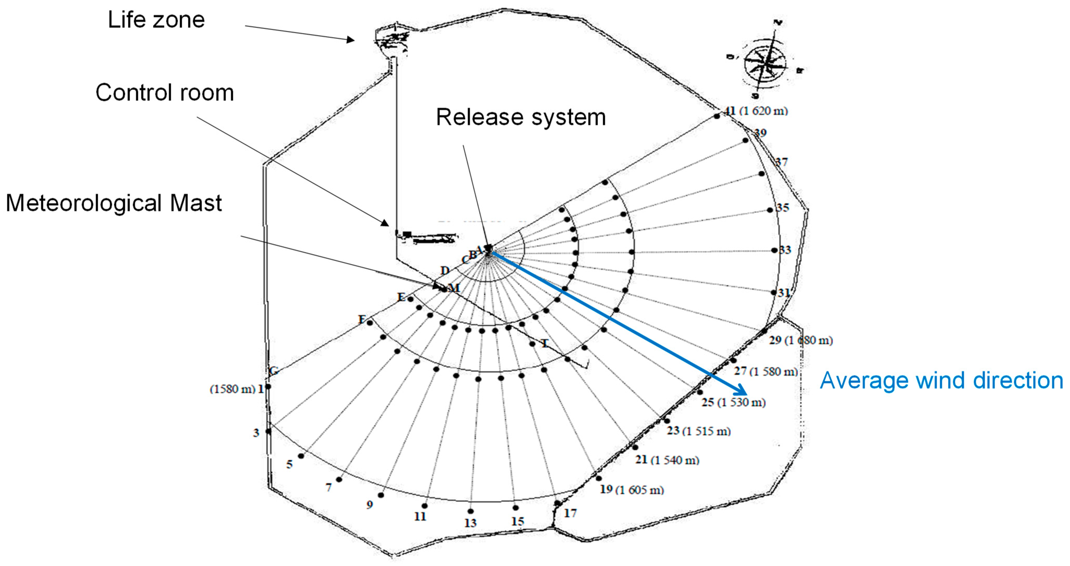
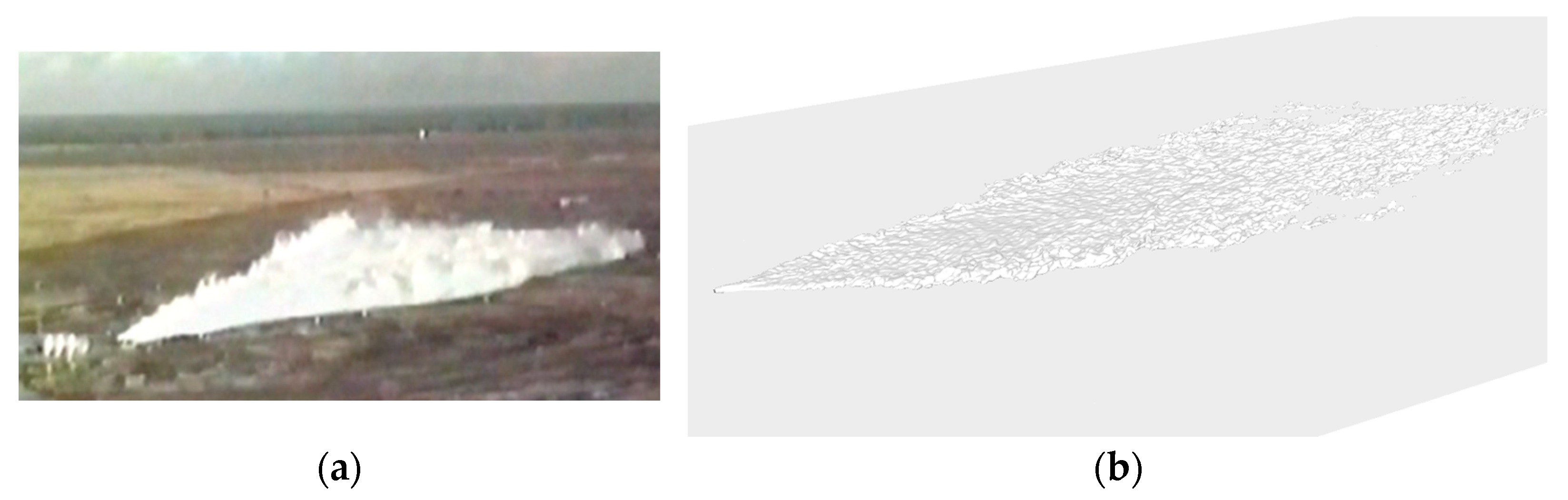
3.1. Description of the Experimental Dataset

Ammonia dispersion field tests performed by INERIS were presented in a previous paper [38]. INERIS conducted real-scale releases of ammonia on the 950-ha flat testing site of CEA-CESTA. Figure 3 shows the whole measurement area.

During the experiments, atmospheric conditions were assessed using a meteorological mast standing at a height of 10 m. The mast was equipped with three cup anemometers positioned at 1.5, 4, and 7 m above the ground, a wind vane at 7 m, and an ultrasonic anemometer at 10 m. Additionally, a weather station was set up near the testing site to measure ambient temperature, relative humidity, and solar flux at 1.5 m above the ground. Sensors were strategically placed in seven arc shapes centred on the release point. Multiple test cases were conducted involving releases with mass flow rates of up to 4.2 kg/s and two-phase releases. For the scope of the present paper, case 4 is considered; it corresponds to a free-field horizontal 10-min release. The mean wind direction is indicated in Figure 3, thanks to the blue line. In this study, an enhanced wind flow analysis is carried out to take into account additional measurements provided by an ultrasonic anemometer (see

Table 1. Ultrasonic anemometer (10 Hz) measurements (over first 5 min of the release) for trial case 4.

Ambient Temperature	Wind Speed (m/s) at 10 m	Friction Velocity: u* (m/s)	Pasquill Stability Class by Determined by the Standard Deviations of the Wind Direction	Monin-Obukhov Lenght (LMO) (−)
14.82 °C	3.24	0.36	C	−166

).

3.2. Atmospheric Dispersion Modelling by “Swift” Model

The widely used dense gas dispersion SLAB has been used to simulate the trial case. It is available for free thanks to the Environmental Protection Agency (EPA). The model can handle horizontal jets [14]; in the far field, a shallow-layer approach is widely used to disperse dense gas according to the observed behaviour of the release. This model is well suited for emergency situations; indeed, it allows us to obtain a swift estimation of effect distances, and it has been used in many comparisons with heavy dispersion gas dispersion campaigns at large scales [14,39]. The model was run in diagnostic mode with the optimum source release terms, knowing the experimental mass flow rate and that experimental observations showed very little rainout deposition on the ground. The flow input is set by the stability Pasquill (see Table 1), according to the sonic anemometer measurements, and a roughness value of z0 = 0.03 m was selected according to the land cover of the experimental site ground (prairie grass).

3.3. Adaptation of the Experimental Atmospheric Signal for CFD Model Inflow

3.3.1. Turbulent Closure and Inlet Boundary Conditions

The RANS CFD simulations were performed using Code_Saturne, which is a general-purpose open source CFD code (www.code-saturne.org) [40]. This method has undergone testing in both flat terrain [41] and obstructed environments [42]. The governing equations are solved based on Boussinesq’s hypothesis. Simulations utilised an adapted k − ε turbulence model for atmospheric flow [43]. The transport equations for turbulent kinetic energy (k) and scalar dissipation rate (ε) account for wind shear and buoyancy effects on k production or dissipation. The latter term is determined by the potential temperature gradient. Indeed, the transport equation for the potential temperature (θ) profile is solved across the domain. The constants used for the k − ε turbulence model in atmospheric flows were modified according to previous research [21]. Here, Cµ = 0.03, following the work of Duynkerke [21], and the value of Cε3 is determined as per [44]: Cε3 = 0 for a stably stratified atmosphere and Cε3 = 1 for an unstably stratified atmosphere, aligning with the specific conditions examined in this study.

The atmospheric stability class is represented by the inflow boundary condition for the velocity, the turbulent kinetic energy k, dissipation of turbulent kinetic energy ε, and the temperature profile. The inlet and the top boundary are specified by the Dirichlet condition. The outlet is a free-outflow condition. The lateral boundaries are symmetry conditions. In previous computational fluid dynamics (CFD) flow simulations [42], it was observed that improved outcomes could be achieved by adjusting the inlet conditions to match measurements for both the mean velocity profile and turbulence intensity. Hence, the formulation for the wind and turbulence profile was selected to achieve a more satisfactory comparison between the CFD inlet conditions and the experimental profile (see Figure 4).

A power law velocity, according to the stability class reported by Barrat [45], i.e., n = 0.16 (stability class C). The scalar dissipation rate profiles is based on the hypothesis that viscous dissipation balances shear production and buoyancy. The inlet profiles of k, ε and the turbulent viscosity, K_m are specified as follows [30]:

$$k(z)=\frac{{{\displaystyle u}\ast }^2}{\sqrt{{{\displaystyle C}}_{\mu }}}\sqrt{1-\frac{z}{L}} \hspace{1em}\epsilon (z)=\frac{{{\displaystyle u}\ast }^3}{\kappa }{(1-\frac{16z}{L})}^{-1/4}(1-\frac{z}{L}) \hspace{1em}{{\displaystyle K}}_m(z)={{\displaystyle C}}_{\mu }\frac{{{\displaystyle k^2(z)}}^{}}{\epsilon (z)}$$

(3)

The LES CFD simulations were achieved using FDS, a freely available CFD code provided by the NIST [46] and initially dedicated to gradient density-based flow modelling. As discussed previously in this paper, the focus for LES is not inside the domain since the main effect of the flow on turbulence is explicitly solved but is for the inlet boundary condition. When using LES, defining a representative turbulent flow field as an inflow boundary condition is an issue. The flow should satisfy prescribed spatial correlations and turbulence characteristics as required by the well-known synthetic eddy method (SEM) [47]. The method used in the present study is based on physical assumptions; it consists of generating a synthetic turbulent velocity signal written as a sum over a finite number of eddies with random intensities and positions. It is based on the observation that large-scale coherent structures in turbulent flows carry most of the Reynolds stresses. More precisely, the method involves the generation and superposition of a large number of random eddies (N), with some control over their statistical properties, and using the following predefined shape function for the velocity fluctuation (see Equation (3) in [47]). These eddies are then transported through an 800 m long rectangular cross-section domain. The resultant, time-dependent flow field taken from a cross-section of this domain can be extracted and imposed as an inlet condition for LES. This method allows the desired Reynolds stress field to be prescribed. Inflow boundaries for the synthetic method available in FDS consist of data given by following experimental results: mean velocity (U_mean), root mean square velocity in x-direction matching with mean wind direction (RMS_x), integral time scale (T_x), integral scale in x-direction (L_x). The inflow mean velocity profile follows an exponential law. The integral length scale may be defined by assuming the advection of turbulent structures by the averaged wind, such as L_x = U_mean × T_x with T_x the observed integral time scale in the x-direction. The atmospheric data used as inflow boundary conditions for the LES approach are presented in

Table 2. Atmospheric input data for LES approach.

Anemometer Altitude (m)	Umean (m/s)	Tx (s)	Lx	RMSx
1.5	2.59	12	31.0	0.72
4	2.94	14	41.1	0.68
7	3.18	20	63.6	0.64
10	3.24	17	55	0.9

. The number of eddies is equal to 1000.

The RMS velocity fluctuation set up at the inlet is isotropic. In other words, the diagonal components of the Reynolds stress are identical, and all others are set to 0. The outlet is a free-outflow condition. The lateral boundaries are symmetry conditions. No temperature profile is set up at the inlet.

3.3.2. Mesh and Numerical Set-Up

The physical domain used is 1300 m × 600 m × 60 m in the x, y, and z directions for RANS and 800 m × 400 m × 40 m for LES. The computational grid consists of approximately 1.2 million hexahedral volume elements for RANS (expanded grid with an expansion ratio lower than 1.2) and 2 million hexahedral volume elements for LES. The minimal space length is 0.5 m, corresponding to cells located close to the ground, and it allows implementation of the source term with 4 cells (see

Table 3. Implementation of a biphasic dense gas source term in CFD code: inlet boundary for CD code (a); characteristics of source term (b) determined by 1-D approach.

Physical Characteristic	Value
Distance between real and artificial release	6 m
Velocity used in the CFD code	25 m/s
Vapor Temp	−50 °C
Section area	1 m²
NH3 mass flow rate:	4.2 kg/s (experimental data)
Air mass flow rate	19.1 kg/s
Total mass flow rate	23.3 kg/s

).

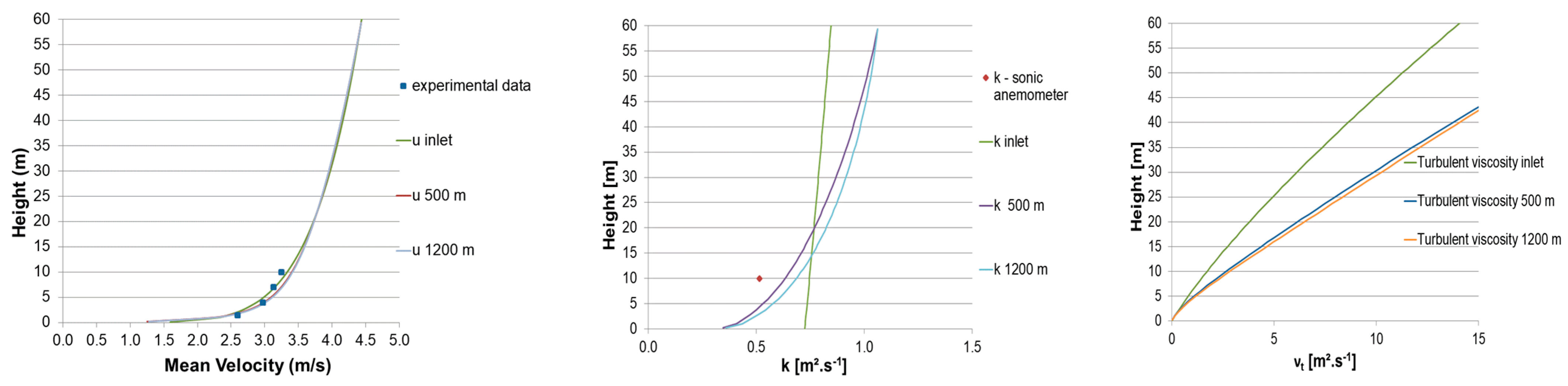
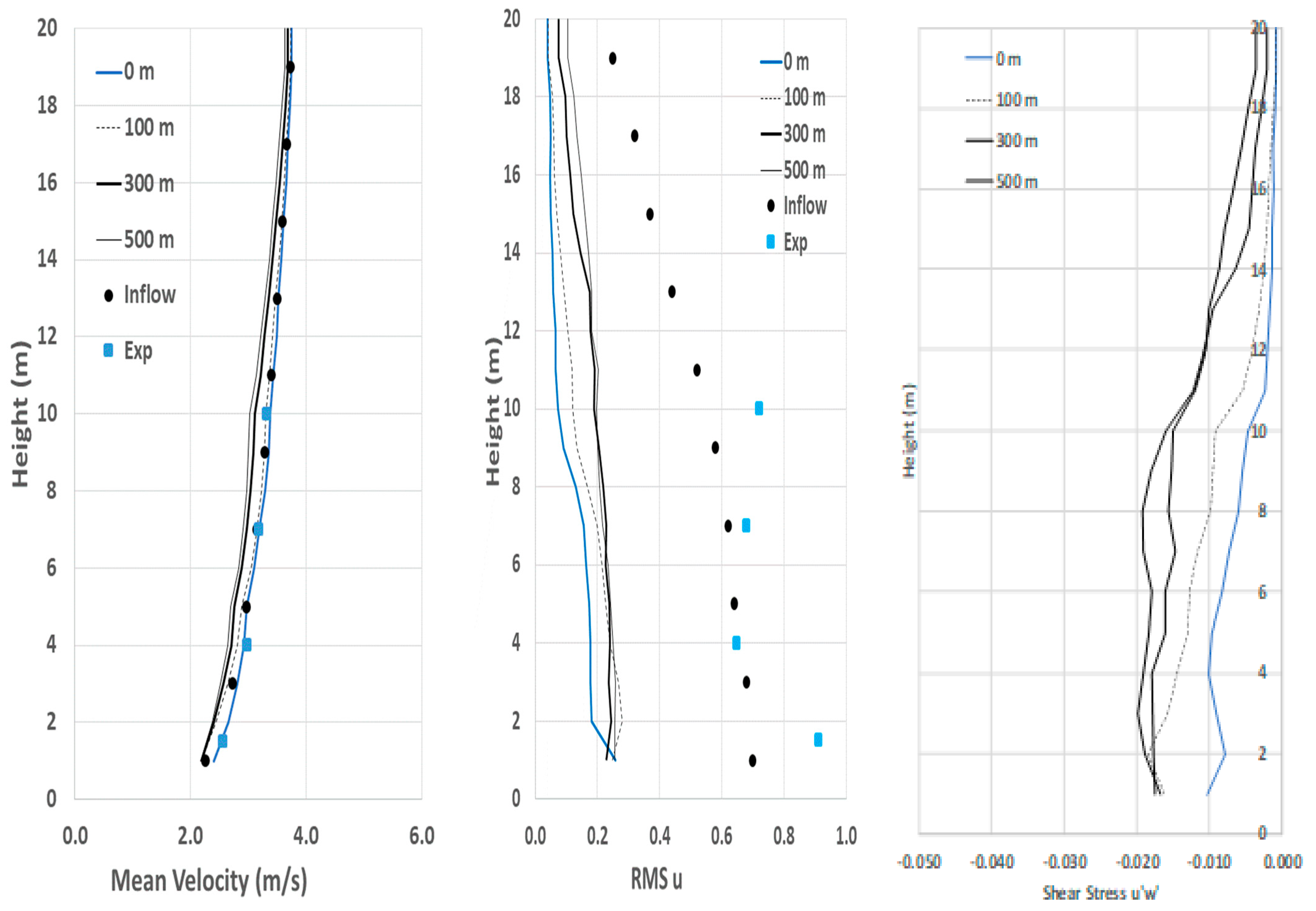
3.3.3. Wind and Turbulence Profile Advection

The initial phase of the entire simulation process involves verifying the accuracy of the modelled wind flow to ensure that a homogeneous atmospheric boundary layer (ABL) is maintained throughout the domain. In the context of the Reynolds-Averaged Navier-Stokes (RANS) approach, the results indicate well-preserved ABL profiles, although there is a decrease in turbulence kinetic energy downstream from the inlet. Challenges expected in the current atmospheric conditions (slightly unstable) were anticipated and have been addressed in prior studies [31,48]. However, the turbulent viscosity profile (see Figure 1) is reasonably sustained close to the ground (z < 5 m). Consequently, it is assumed that the disparity between ABL profiles at the inlet and outlet has a minor impact on dispersion predictions. Furthermore, the theoretical profile used to establish input turbulence marginally overestimates the measurement taken by the sonic anemometer at a height of 10 m (see Figure 4). This suggests that the turbulence levels simulated by Code_Saturne could be deemed close to those observed during the test.

Figure 5 shows the flow characteristics obtained with LES approach at different x-positions and compared against inflow conditions and experimental data.

The mean velocity is well maintained in the domain. However, turbulence decreases rapidly in the first part of the calculation domain, but RMS profiles are sustained in a steady way. This turbulence decrease was expected [49] and explained the underestimation of friction velocity when compared to experimental data. Other strategies exist to set up a LES [50] model, but to the best of the authors’ knowledge, few studies have been carried out on an industrial site scale. These clearly highlight that, while LES offers a theoretically relevant approach for atmospheric dispersion since it natively considers the flow properties, the practical use is more complex and challenging due to the large domain to be modelled and the interaction of the flow with the ground to obtain an equilibrate turbulent profile.

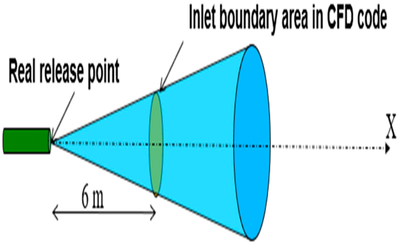
3.4. Implementation of a Biphasic Dense Gas Source Term

FDS and Code_Saturne cannot directly deal with high-speed multi-phase releases. Then, an equivalent source term (see Table 3) was implemented at a distance from the orifice to bypass this limitation, thus leading to moderate velocity and a weak liquid fraction that can be readily handled by CFD code. Knowing the ammonia experimental mass flow rate, the general properties of the fluid in the very near field are obtained by means of a weighting operation between the gas and the liquid near the orifice within the homogeneous model (HEM) [37]. This latter is combined with the Papadourakis et al. [51] approach to simulate a biphasic jet to compute a source term and set up a gaseous source term equivalent. It is then implemented as a monophasic equivalent term source in FDS and Code_Saturne simulation. A summary of the latter is given in Table 3.

3.5. Synthesis of Model Inputs

Table 4. Harmonised and specific input data for SLAB model and CFD approach.

Model	Dispersion Model	Atmospheric Flow Input		Source Term
		Common	Specific	Common	Specific
SLAB	Shallow layer	Mean velocity at reference height. Ground roughness of 0.03 m	Pasquil Stability class	NH3 mass flow rate of 4.2 kg/s,1 m high	Orifice release conditions: NH3 Mass flow rate of 4.2 kg/s, 0.6 liquid fraction
Code_Saturne	CFD, RANS		Turbulent kinetic energy and dissipation and temperature profile (not shown) based on experimental friction velocity, LMO and heat flux		Pseudo-source conditions: Equivalent gas source term located at 6 m from orifice, Total mass flow rate of 23.3 kg/s Surface area of 1 m²
FDS	CFD, LES		Isotropic integral time, length scale and RMS based on experimental data

summarises the data used as inflow boundary conditions and for emission source terms for the three approaches used in this study. This table points out the common inputs that are used and the discrepancies that appear before running the simulation itself, just due to setting the calculation.

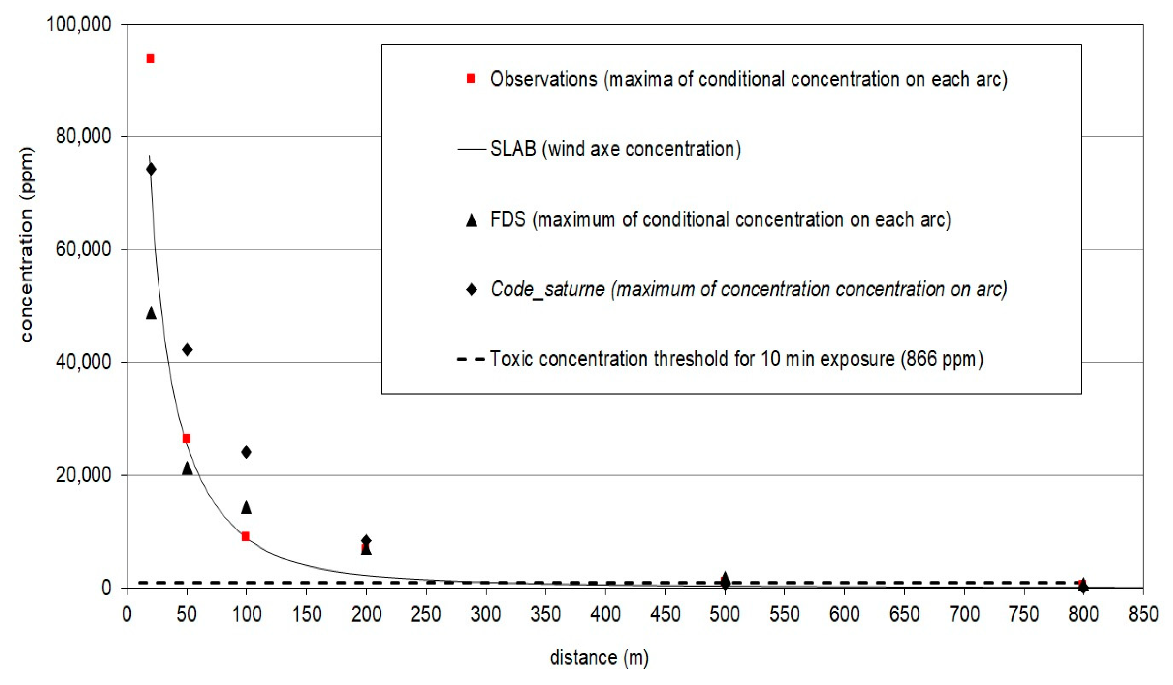
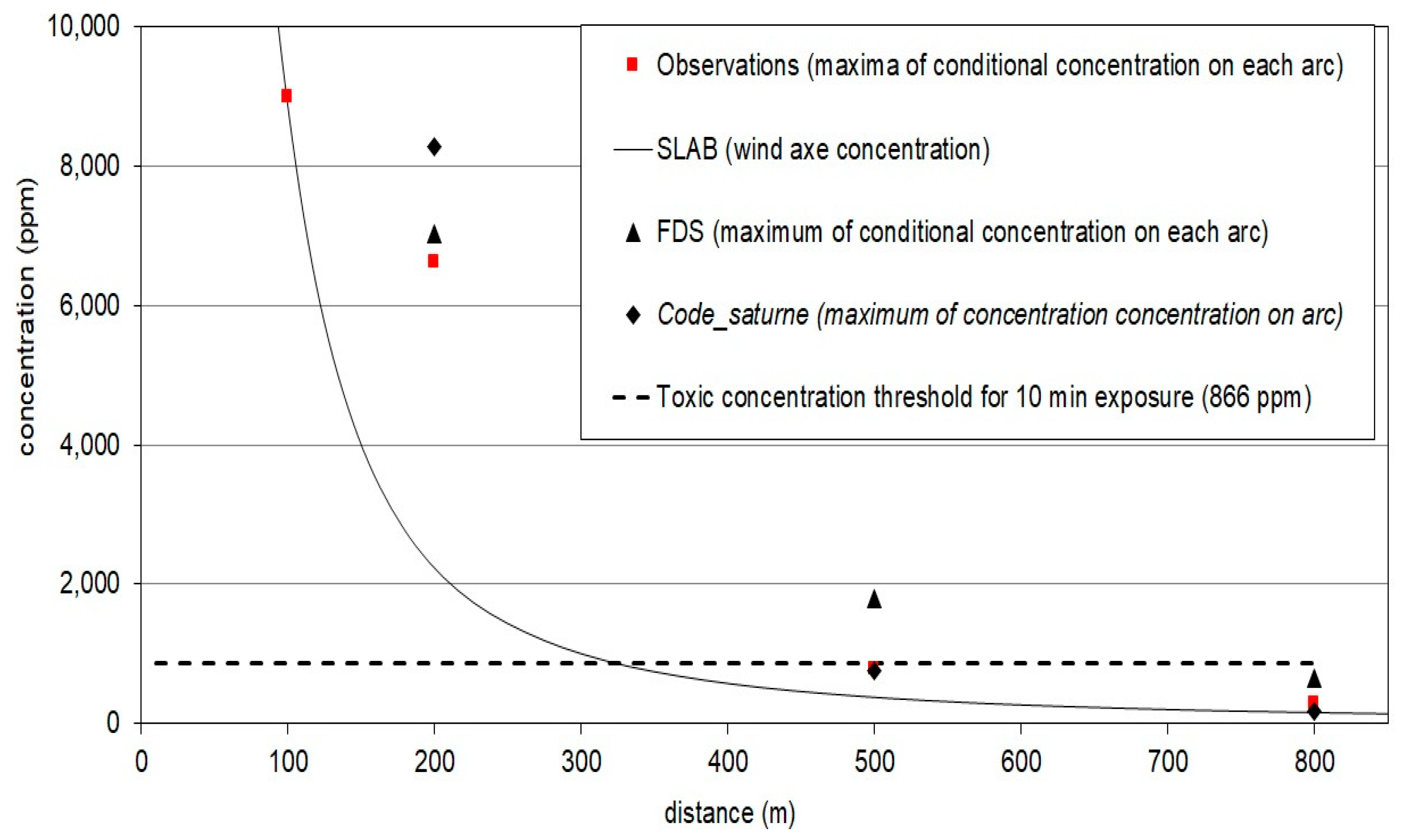
3.6. Comparison of Measured Concentrations with Atmospheric Dispersion Modelling Results

One of the key results provided by AT&D is the concentration profile along the wind axis. Indeed, it allows for a swift estimation of safety distance by cross-referencing the toxic concentration threshold. A comparison between the simulation results obtained with the three models and experimental concentration data at z = 1 m along the main wind axis is presented in Figure 6. The set of experimental observations corresponds to maxima of mean conditional concentration values (red square in Figure 6, Figure 7 and Figure 8) observed by sensors for each arc. According to the definition of previous studies [52,53], these concentrations are determined from the mean of non-zero concentrations during the lifetime of the signal. The sensors involved in trial 4 are located on the 23, 25, and 25 axes (see Figure 3). The corresponding concentrations for the CFD model (at z = 1 m) are presented for a rigorous comparison. The averaging time roughly corresponds to the exposition time period defined by the arrival time and departure time of the cloud. SLAB results correspond to concentrations obtained with an averaging time of 600 s at a height where maxima are obtained (in this case at 0 m < z < 1 m) along the wind axis.

It can be noticed that global tendencies are quite well reproduced by all approaches. The concentrations decrease along the mean wind axis, modelled by SLAB, and the observations can be deemed in good accordance, particularly in the near field (x < 200 m). This is to be put into relief with the easy use of this kind of model, particularly when it is needed to obtain an order of magnitude in a emergency situation. However, in the far field (x > 200 m) (see Figure 7), this swift model underestimates the level of concentration illustrated by the threshold of toxicity for 10 min of exposure (866 ppm). It results in a corresponding distance that is roughly underestimated by a factor of ~1.5.

In the context of both Reynolds-Averaged Navier-Stokes (RANS) and Large Eddy Simulation (LES) approaches, these findings hold promise in tackling the challenge of describing both near-field and far-field releases. Nevertheless, the model tends to slightly overestimate the measurements, specifically within the near field (50 m < x < 200 m) for the RANS model and in the far field (x > 200 m) for the LES model. One plausible explanation could be the insufficient level of mixing resulting from the atmospheric flow. Previous studies [40,49] have highlighted the potential weakness of the k − ε and LES turbulence models in addressing this issue.

Visual observations show clearly that the ammonia cloud (see Figure 9) is dense and moving near the ground, far from the source. The amount of initial liquid fraction within the experimental cloud is much larger than the critical value, estimated between 4 and 8% of the total mass of ammonia for air at 293 K by previous studies [54], such that the cloud remains denser than the surrounding air regardless of the humidity of the air.

The modelled cloud of ammonia by FDS behaves well as a dense gas around several hundred metres. A rough comparison between FDS modelling results and experimental observations shows that the whole shape of the modelled cloud at 500 ppm is in good accordance with experimental observations see Figure 9) that indicated the plume is visible until approximately until 500 m [55]. This figure typically shows that the modelling tool is able to reproduce, with quite good agreement, the typical shape of the cloud. This level of concentration corresponds to the toxic threshold (French Acute Toxicity Threshold Values) for irreversible effects on human health in the case of 30 min of exposure. That length of exposure can be deemed a representative exposure time for a lot of unintended toxic release scenarios within an industrial risk assessment context.

According to Carruthers et al. [55], it can be considered that the cloud is visible as soon as the liquid water content (r_liq) is greater than 10⁻⁵ kg/kg. A very simplistic and rough estimate can be carried out using the method proposed by these authors. Starting from an initial mixing ratio value at the release point that is around 220 g of NH₃ by kg of air (see Table 3), it appears that for a dilution of 500 ppm, the mixing ratio value of the cloud, r_cl, is around 43 g of NH₃ by kg of air. For an ambient humidity of 82% (trial 4), the saturated mixing ratio, r_sat, is around 10 g/kg. It turns out that r_liq = r_cl − r_sat is >> 10⁻⁵ kg/kg, as the CFD modelling result combined with a simplistic estimate tends to confirm that the cloud is visible at a level of 500 ppm in the trial 4 ambient conditions. The severe difference in terms of plume visibility would be obtained in cases of distinct ambient conditions; this issue has been put forward by recent research projects [56].

Comparisons between CFD model results and observations are presented for each arc concentration sensor in Figure 8.

It appears that simulation by FDS overestimates far field concentration, while simulation by Code_Saturne underestimates the plume width. This comparison is a good illustration of the difficulty of assessing all the phenomena both in the near field and the far field [57]. Bearing in mind the use of an equivalent gas source term, these results are very promising. This study should be considered an essential stage for validating the use of the CFD model in the context of regulatory studies where the need to assess an obstructed environment will be of primary importance.

3.7. Outcomes for Best Practices within the Regulatory Context

The modelling of the experimental massive release has highlighted practices about data processing and sub-model choice and their influence on the results. The main outcomes to bear in mind in the regulatory context are synthesised in this sub-chapter.

The turbulence and wind inlet profiles for various stability classes are of such significance that they must be formulated based on consensus-established equations for Swift model and CFD codes. Indeed, they directly impact pollutant atmospheric dispersion by means of turbulence diffusion and advection phenomena. Generating these profiles (see Section 3.3.1) is intrinsically related to a unique roughness value for the wind velocity value at the height and friction velocity value. As illustrated in the previous section, the two first parameters, when combined with the Pasquill class, are generally direct inputs for Swift models. The friction velocity value is a sensitive parameter, as it largely influences both turbulence and wind profile. This reinforces the need, in the regulatory context, to propose a common method to estimate its value, starting from the simplest data set. A single roughness height may characterise the entire area of interest for an accidental release on a local scale. An enhanced study, based on a statistically wider wind study of the site, would be necessary to assess this value, which is generally sensitive for atmospheric dispersion modelling. The choice of inlet profile formulations for RANS CFD should be made consistently with the choice of sub-model turbulence for RANS approach [26,31] to reach a satisfactory equilibrium state for ABL. For the LES CFD approach, a more complete turbulence set of data can potentially be assessed, as illustrated in Table 4. In a regulatory context with a minimum set of data that allows the building of a turbulent profile for the RANS model, it would be possible to assess the typical turbulent length scales that made it possible to build the required data for LES profiles, as demonstrated in Section 3.3.1. The choice of sub-model comes next to the crucial choice about the mesh requirements.

The harmonisation in CFD codes of an equivalent source term is feasible by means of the implementation of an identical term source that is fully gaseous.

4. Conclusions

Within the context of industrial risk assessment, the prediction of the impact area (thermal, overpressure, and toxic effects) is required. Atmospheric dispersion models are then used to predict distances or impacted zones by toxic or flammable products, for regulatory studies such as land use planning, or for emergency management.

A review of practices for AT&D in regulatory studies within the industrial risk assessment context has been discussed within the present study. This review highlights the reasons that can explain these discrepancies between computation approaches to assess toxic consequences in the neighbourhood of industrial facilities.

Several AT&D models of different s, shallow-layer, CFD-RANS, and CFD-LES, have been used to model a large-scale experimental ammonia release. This experimental ammonia case was targeted because it represents an unobstructed environment, which is within the application domain of all AT&D model types. Based on experimental observation analysis, flow input data and source terms of different levels of complexity have been set up for each approach. The same equivalent gas term located has been set for LES and RANS approaches to harmonising practices. Expected difficulties to maintain the turbulence level along the flat domain have been encountered for CFD approaches. Considering the inherent complexity of modelling and simulating the atmospheric turbulence, the predicted concentration is in good agreement with experimental data for both the RANS and LES approaches.

Harmonisation of input data for flow and boundary layer simulation between the Swift model and more sophisticated models remains a major issue within the context of regulatory studies. The authors of the present study promote research and development to support this objective, particularly for the LES approach.

References

1. Cavallaro, A.; Tebaldi, G.; Gualdi, R. Analysis of Transport and Ground Deposition of the TCDD Emitted on 10 July 1976 from the ICMESA Factory (Seveso, Italy). Atmos. Environ. 1967, 16, 731–740. [Google Scholar] [CrossRef]
2. Havens, J.; Walker, H.; Spicer, T. Bhopal Atmospheric Dispersion Revisited. J. Hazard. Mater. 2012, 233, 33–40. [Google Scholar] [CrossRef] [PubMed]
3. Folch, A.; Barcons, J.; Kozono, T.; Costa, A. High-Resolution Modelling of Atmospheric Dispersion of Dense Gas Using TWODEE-2.1: Application to the 1986 Lake Nyos Limnic Eruption. Nat. Hazards Earth Syst. Sci. 2017, 17, 861–879. [Google Scholar] [CrossRef]
4. Al-Shanini, A.; Ahmad, A.; Khan, F. Accident Modelling and Analysis in Process Industries. J. Loss Prev. Process Ind. 2014, 32, 319–334. [Google Scholar] [CrossRef]
5. Lenoble, C.; Durand, C. Introduction of frequency in France following the AZF accident. J. Loss Prev. Process Ind. 2011, 24, 227–236. [Google Scholar] [CrossRef]
6. Carissimo, B.; Castelli, S.T.; Tinarelli, G. JRII Special Sonic Anemometer Study: A First Comparison of Building Wakes Measurements with Different Levels of Numerical Modelling Approaches. Atmos. Environ. 2021, 244, 117798. [Google Scholar] [CrossRef]
7. Jacob, J.; Merlier, L.; Marlow, F.; Sagaut, P. Lattice Boltzmann Method-Based Simulations of Pollutant Dispersion and Urban Physics. Atmosphere 2021, 12, 833. [Google Scholar] [CrossRef]
8. Turner, D.B. Workbook of Atmospheric Dispersion Estimates; Publication No. 999, AP26; U.S. Public Health Service, Division of Air Pollution: Washington, DC, USA, 1970.
9. Copelli, S.; Barozzi, M.; Fumagalli, A.; Derudi, M. Application of a Gaussian Model to Simulate Contaminants Dispersion in Industrial Accidents. Chem. Eng. Trans. 2019, 77, 799–804. [Google Scholar] [CrossRef]
10. Doury, A. Vade-Mecum des Transferts Atmosphériques; DSN report n°440. 1981. Available online: https://www.radioprotection.org/articles/radiopro/ref/2011/06/radiopro_icrer_46668/radiopro_icrer_46668.html (accessed on 20 September 2023).
11. Hanna, S.R.; Briggs, G.A.; Hosker, R.P., Jr. Handbook on Atmospheric Diffusion; Technical Information Center U.S. Department of Energy: Oak Ridge, TN, USA, 1982.
12. Pasquill, F. The estimation of the dispersion of windborne material. Meteorol. Mag. 1961, 90, 33–49. [Google Scholar]
13. Witlox, H.W.M. PHAST 6.0—Unified Dispersion Model—Consequence Modelling Documentation; DNV: Katy, TX, USA, 2000. [Google Scholar]
14. Ermak, D.L. User’s Manual for SLAB: An Atmospheric Dispersion Model for Denser Than Air Releases; UCRL-MA-105607; Lawrence Livermore National Laboratory: Livermore, CA, USA, 1990.
15. Sidik, N.A.C.; Yusuf, S.N.A.; Asako, Y.; Mohamed, S.B.; Japar, W.M.A.A. A Short Review on RANS Turbulence Models. CFD Lett. 2020, 12, 83–96. [Google Scholar] [CrossRef]
16. Garnier, E.; Adams, N.; Sagaut, P. Large Eddy Simulation for Compressible Flows; Springer: Berlin/Heidelberg, Germany, 2009. [Google Scholar] [CrossRef]
17. Pope, S. Ten questions concerning the large-eddy simulation of turbulent flows. New J. Phys. 2004, 6, 35. [Google Scholar] [CrossRef]
18. Baumann-Stanzer, K.; Leitl, B.; Trini Castelli, S.; Milliez, C.M.; Berbekar, E.; Rakai, A.; Fuka, V.; Hellsten, A.; Petrov, A.; Efthimiou, G.; et al. Evaluation of local-scale models for accidental releases in built environments—Results of the “Michelstadt exercise” in COST Action ES1006. In Proceedings of the 16th International Conference on Harmonisation within Atmospheric Dispersion Modelling for Regulatory Purposes, Varna, Bulgaria, 8–11 September 2014. [Google Scholar]
19. Detering, H.W.; Etling, D. Application of the turbulence model to the atmospheric boundary layer. Bound.-Layer Meteorol. 1985, 33, 113–133. [Google Scholar] [CrossRef]
20. Rodi, W. Turbulence Models and Their Application in Hydraulics: A State-of-the-Art Review, 3rd ed.; Routledge: London, UK, 1993. [Google Scholar]
21. Duynkerke, P. Application of the k-ε turbulence closure model to the neutral and stable atmospheric boundary layer. J. Atmos. Sci. 1988, 45, 865–880. [Google Scholar] [CrossRef]
22. Smagorinsky, J. General circulation experiments with the primitive equations. Mon. Weather. Rev. 1963, 91, 99–164. [Google Scholar] [CrossRef]
23. Stull, R.B. An Introduction to Boundary Layer Meteorology; Springer Science & Business Media: Berlin, Germany, 1988. [Google Scholar]
24. Montero, G.; Rodríguez, E.; Oliver, A.; Calvo, J.; Escobar, J.M.; Montenegro, R. Optimisation technique for improving wind downscaling results by estimating roughness parameters. J. Wind. Eng. Ind. Aerodyn. 2018, 174, 411–423. [Google Scholar] [CrossRef]
25. Golder, D. Relations among stability parameters in the surface layer. Bound.-Layer Meteorol. 1972, 3, 47–58. [Google Scholar] [CrossRef]
26. Guide de Bonnes Pratiques Pour la Réalisation de Modélisations 3D pour des Scénarios de Dispersion Atmosphérique en Situation Accidentelle. Rapport de Synthèse des Travaux du Groupe de Travail National. Available online: https://aida.ineris.fr/sites/aida/files/guides/Guide_Bonnes_Pratiques_V2.02_RNT.pdf (accessed on 23 February 2011).
27. Lacome, J.-M.; Truchot, B. Harmonization of practices for atmospheric dispersion modelling within the framework of risk assessment. In Proceedings of the 15th Conference on “Harmonisation within Atmospheric Dispersion Modelling for Regulatory Purposes, Madrid, Spain, 6–9 May 2013. [Google Scholar]
28. Gryning, S.; Batchvarova, E.; Brümmer, B.; Jorgensen, H.; Larsen, S. On the extension of the wind profile over homogeneous terrain beyond the surface boundary layer. Bound.-Layer Meteorol. 2007, 124, 251–268. [Google Scholar] [CrossRef]
29. Commission for the Prevention of Disasters Caused by Hazardous Materials. TNO—Yellow Book: “Methods for Calculation of Physical Effects”; CPR 14E; Ministerie van Verkeer en Waterstaat: The Hague, The Netherlands, 1996.
30. Vendel, F. Modélisation de la Dispersion Atmosphérique en Présence D’obstacles Complexes: Application à L’étude de Sites Industriels. Ph.D. Thesis, University of Lyon, Lyon, France, 2011. [Google Scholar]
31. Batt, R.; Gant, S.E.; Lacome, J.-M.; Truchot, B. Modelling of stably-stratified atmospheric boundary layers with commercial CFD software for use in risk assessment. In Proceedings of the 15th International Symposium on Loss Prevention and Safety Promotion in the Process Industries, Freiburg, Germany, 5–8 June 2016. [Google Scholar]
32. Blocken, B.; Stathopoulos, T.; Carmeliet, J. CFD simulation of the atmospheric boundary layer: Wall function problems. Atmos. Environ. 2007, 41, 238–252. [Google Scholar] [CrossRef]
33. Britter, R.; Weil, J.; Leung, J.; Hanna, S. Toxic industrial chemical (TIC) source emissions modeling for pressurized liquefied gases. Atmos. Environ. 2011, 45, 1–25. [Google Scholar] [CrossRef]
34. Calay, R.; Holdo, A. Modelling the dispersion of flashing jets using CFD. J. Hazard. Mater. 2008, 154, 1198–1209. [Google Scholar] [CrossRef]
35. Lacome, J.; Lemofack, C.; Jamois, D.; Reveillon, J.; Duret, B.; Demoulin, F. Experimental data and numerical modeling of flashing jets of pressure liquefied gases. Process. Saf. Prog. 2020, 40, e12151. [Google Scholar] [CrossRef]
36. Kelsey, A. CFD Modeling of Propane Flashing Jets: Simulation of Flashing Propane Jets; Health & Safety Laboratory, UK: Buxton, UK, 2002.
37. Britter, R.E. Dispersion of Two-Phase Flashing Releases; CERC Ltd.: Leicester, UK, 1995. [Google Scholar]
38. Bouet, R.; Duplantier, S.; Salvi, O. Ammonia large scale atmospheric dispersion experiments in industrial configurations. J. Loss Prev. Process. Ind. 2005, 18, 512–519. [Google Scholar] [CrossRef]
39. Tørnes, J.A.; Vik, T. Comparison of some commercial dispersion models for heavy gas releases. In Proceedings of the 18th International Conference on Harmonisation within Atmospheric Dispersion Modelling for Regulatory Purposes, Bologna, Italy, 9–12 October 2017. [Google Scholar]
40. Demael, E.; Carissimo, B. Comparative Evaluation of an Eulerian CFD and Gaussian Plume Models Based on Prairie Grass Dispersion Experiment. J. Appl. Meteorol. Climatol. 2008, 47, 888–900. [Google Scholar] [CrossRef]
41. Archambeau, F.; Mechitoua, N.; Sakiz, M. Code_Saturne: A finite volume code for the computation of turbulent incompressible flows—Industrial applications. Int. J. Finite Vol. 2004, 1, 1–62. [Google Scholar]
42. Milliez, M.; Carissimo, B. Numerical simulations of pollutant dispersion in an idealized urban area, for different meteorological conditions. Bound.-Layer Meteorol. 2007, 122, 321–342. [Google Scholar] [CrossRef]
43. Xiao, W. Experimental and Numerical Study of Atmospheric Turbulence and Dispersion in Stable Conditions and in Near Field at a Complex Site. Ph.D. Thesis, Universite de Paris-Est-Marne-la-Vallee, Paris, France, 2016. [Google Scholar]
44. Viollet, P.L. On the numerical modeling of stratified flows. In Physical Processes in Estuaries; Springer: Berlin/Heidelberg, Germany, 1988; pp. 257–277. [Google Scholar]
45. Barratt, R. Atmospheric Dispersion Modelling: A Practical Introduction; Business & Environmental Practitioner; Routledge: London, UK, 2001. [Google Scholar]
46. McGrattan, K.B. Fire Dynamics Simulator (Version 4): Technical Reference Guide NIST Special Publication 1018; NIST: Washington, DC, USA, 2005.
47. Jarrin, N. Synthetic Inflow Boundary Conditions for the Numerical Simulation of Turbulence. Ph.D. Thesis, University of Manchester, Manchester, UK, 2008. [Google Scholar]
48. Gorlé, C.; van Beeck, J.; Rambaud, P.; Van Tendeloo, G. CFD modelling of small particle dispersion: The influence of the turbulence kinetic energy in the atmospheric boundary layer. Atmos. Environ. 2009, 43, 673–681. [Google Scholar] [CrossRef]
49. Hanna, S.R.; Tehranian, S.; Carissimo, B.; Macdonald, R.W.; Lohner, R. Comparisons of Model Simulations with Observations of Mean Flow and Turbulence within Simple Obstacle Arrays. Atmos. Environ. 2002, 36, 5067–5079. [Google Scholar] [CrossRef]
50. Estrada, J.M. Numerical Simulation of Atmospheric Dispersion: Application for Interpretation and Data Assimilation of Pollution Optical Measurements. Ph.D. Thesis, University of Lyon, Lyon, France, 2022. [Google Scholar]
51. Papadourakis, A.; Caram, H.S.; Barner, C.L. Upper and lower bounds of droplet evaporation in two-phase jets. J. Loss Prev. Ind. 1993, 4, 93–101. [Google Scholar] [CrossRef]
52. Yee, E.; Biltoft, C.A. Concentration Fluctuation Measurements in a Plume Dispersing Through a Regular Array of Obstacles. Bound.-Layer Meteor. 2004, 111, 363–415. [Google Scholar] [CrossRef]
53. Wilson, D.J. Concentration Fluctuations and Averaging Time in Vapor Clouds; Wiley: Hoboken, NJ, USA, 1995. [Google Scholar]
54. Haddock, S.R.; Williams, R.J. The density of an ammonia cloud in the early stages of atmospheric dispersion. J. Chem. Technol. Biotechnol. 1979, 29, 655–672. [Google Scholar] [CrossRef]
55. Dysters, S.J.; Ellis, K.L. ADMS 3. Plume Visibility by DJ Carruthers; CERC: Leicester, UK, 2005. [Google Scholar]
56. Fox, S.; Hanna, S.; Mazzola, T.; Spicer, T.; Chang, J.; Gant, S. Overview of the Jack Rabbit II (JR II) field experiments and summary of the methods used in the dispersion model comparisons. Atmos. Environ. 2022, 269, 118783. [Google Scholar] [CrossRef]
57. Leroy, G.; Lacome, J.-M.; Truchot, B.; Joubert, L. Harmonization in CFD Approaches to Assess Toxic Consequences of Ammonia Releases. In Proceedings of the 17th International Conference on Harmonisation within Atmospheric Dispersion Modelling for Regulatory Purposes, Budapest, Hungary, 9–12 May 2016. [Google Scholar]
Figure 1. Main stages to simulate atmospheric dispersion of an accidental release (toxic or flammable release) on an industrial site for regulatory studies and emergency management; black boxes represent the whole set-up for the swift and CFD model, green circles represent input data, red circles and red boxes represent intermediate calculation steps, blue boxes represent the intermediate and final result.
Atmosphere 14 01605 g001
Figure 2. Schematic view of the simplified source term for CFD approach for massive release studied in Section 3.
Atmosphere 14 01605 g002
Figure 3. The whole measurement area in CEA-CESTA for the ammonia experimental test cases; sensor arcs locations (distances from the release system: 20 m, 50 m, 100 m, 200 m, 500 m, 800 m, and 1700 m for corresponding referenced letters A, B, C, D, E, F, G); mean wind direction of trial 4 is indicated by the blue arrow.
Atmosphere 14 01605 g003
Figure 4. Predicted results for the flow ABL profiles at the inlet (x = −100 m), center, and outlet of the domain with RANS CFD code.
Atmosphere 14 01605 g004
Figure 5. Flow characteristics against inflow conditions (x = −100 m) and experimental data—LES approach.
Atmosphere 14 01605 g005
Figure 6. Comparison between simulation results and maxima of experimental concentration for each sensor’s arc data.
Atmosphere 14 01605 g006
Figure 7. Comparison between simulation results and experimental concentration data in the far field.
Atmosphere 14 01605 g007
Figure 8. Comparison between simulation results (FDS: continuous line; Code_Saturne: dotted line) and experimental concentration for each arc: (a) circle arc “A” of receptors located at 20 m, (b) circle arc “B” at 50 m, (c) circle arc “C” at100 m, (d) circle arc “D” at 200 m, (e) circle arc “E” at 500 m, (f) circle arc “F” at 800 m.
Atmosphere 14 01605 g008aAtmosphere 14 01605 g008b
Figure 9. Comparison between the overall form of the experimental cloud shape and FDS simulation results: (a) photography of ammoniac cloud during trial 4 release; (b) iso-surface of ammonia simulated concentration (500 ppm).
Atmosphere 14 01605 g009