Article

Extended-Range Forecast of Regional Persistent Extreme Cold Events Based on Deep Learning

1
Institute of Artificial Intelligence for Meteorology, Chinese Academy of Meteorological Sciences, Beijing 100081, China
2
State Key Laboratory of Severe Weather, Chinese Academy of Meteorological Sciences, Beijing 100081, China
3
Xiangtan Meteorological Bureau, Xiangtan 410118, China
*
Author to whom correspondence should be addressed.
Atmosphere 2023, 14(10), 1572; https://doi.org/10.3390/atmos14101572
Submission received: 17 August 2023 / Revised: 11 October 2023 / Accepted: 13 October 2023 / Published: 17 October 2023
(This article belongs to the Section Atmospheric Techniques, Instruments, and Modeling)

Abstract

:
Regional persistent extreme cold events are meteorological disasters that cause serious harm to people’s lives and production; however, they are very difficult to predict. Low-temperature weather systems and their effects have a significant low-frequency oscillation period (10–20 d and 30–60 d). This paper uses deep learning to analyze the extended-range time scale and predict regional persistent extreme cold events. The dominant low-frequency oscillation components of cold events are obtained via wavelet transform and Butterworth filtering. The low-frequency oscillation component is decomposed via empirical orthogonal function decomposition to extract the main spatial mode and time coefficient. A convolutional neural network is used to establish the correlation between large-scale circulations and the time coefficient of the low-frequency oscillation component of the lowest temperature. The proposed deep learning model exhibits good prediction accuracy for regional persistent extreme cold events with low-frequency oscillations.

1. Introduction

With the intensification of global warming, persistent extreme cold events are occurring more frequently [1,2,3]. The persistent cold rain and snow disasters in southern China in 2008 [4], persistent cold events in northern China in 2009, and continuous extreme cold weather in Eurasia in 2012 have caused substantial harm to transportation and people’s production and life.
Cold weather events can be categorized as cold air, cold wave, and extreme cold events. The National Climate Center of the China Meteorological Administration (CMA) uses the following method to define extreme cold events. The lowest temperature of a specific day and the temperatures 5 days before and after that day are related. The temperatures are sorted in ascending order, and the 10th percentile is considered the extreme threshold of the station. An extreme cold event is characterized by a temperature lower than the extreme threshold in the same period of the year within the normal climate period. A cold wave event is defined as a 24 h drop in the daily minimum temperature greater than or equal to 8 °C, a 48 h drop in temperature greater than or equal to 10 °C, or a 72 h drop in temperature greater than or equal to 12 °C and a daily minimum temperature drop below 4 °C. Regional persistent extreme cold events (RPECEs) are primarily cold wave events. According to the statistics of the National Climate Center, most cold wave events (approximately 89%) are not RPECEs because the minimum temperature of a cold wave event may be greater than the extreme threshold in the same period of the year; thus, a cold wave does not constitute a persistent extreme cold event.
Cold waves occur more frequently in winter. It is generally believed that they are caused by the collapse of the high-pressure area in the Ural region or the re-establishment of the East Asian trough, causing cold air to invade northern China from the southward low-pressure trough [5]. The key circulation system that causes different RPECEs compared to cold waves is the large oblique ridge over the Eurasian continent [6] that extends from the Caspian Sea to the Bering Strait. A cold wave occurs when the high-latitude two-wave structure is transformed into a three-wave structure, and the wave train of the Okhotsk Sea declines; the duration is usually 2–3 d. However, the oblique ridge does not form three waves but slowly changes to a larger scale; therefore, its duration is longer [7].
On the other hand, the slow change in large-scale oblique ridges with longer time scales corresponding to RPECEs is the reason for the predictability of the extended range of these events. Therefore, the changes in the circulation of the lower tropospheric atmosphere can be analyzed dynamically to predict RPECEs. Although the cold wave formation can be theoretically predicted similarly, the predictable upper limit is often only 7–8 d, much shorter than the extended-range forecast. Therefore, many cold waves are difficult to predict for longer periods of time [8].
Existing studies on the extended period prediction of temperature and precipitation primarily used statistical or machine learning methods. Yang [9,10] used a principal component–complex autoregressive model and an extended complex autoregressive model to establish a relationship between V850 hPa, T850 hPa, and the forecast quantity for the daily low-frequency component of precipitation and average temperature in the lower reaches of the Yangtze River. Hsu et al. [11,12] established a space–time projection method (STPM) model, based on which Zhu et al. [13] used augmented singular value decomposition (SVD) to predict the extended period of winter surface air temperature and extreme cold weather. They used seven predictors (T850, temperature advection, sea level pressure, 500 hPa vertical motion, H200, SH700, and the time coefficient of the surface air temperature space mode) and calculated their weighted average to obtain one predictor. Lee et al. [14] used historical data to estimate the probability of extremely heavy precipitation for different phases in different months of the Boreal summer intraseasonal oscillation (BSISO) index in the Asian summer monsoon region. Lei et al. [15] utilized a convolutional neural network (CNN) to obtain the future hourly time coefficients of the previous forecast factors (H200, H500, and outward long-wave radiation (OLR)). They used the first K spatial modes of the daily maximum temperature data and synthesized the spatial modes and time coefficient. Wu et al. [16] developed a dynamical-statistical forecasting model (DPSM) to forecast precipitation in an extended period. Augmented SVD was used to establish an equation describing the relationship between the SVD time coefficient and the predicted measurements for the predictors of different historical pentads (OLR, U850, U200, H850, H500, H200, SH700, and SLP). The dynamic and SVD modes were coupled, and the projected time coefficient was used in the linear equation to obtain the predictions. Zhang et al. [17] used SVD to obtain a coupled spatial mode, the time coefficient of the precipitation field, and the predictors of tropical OLR and mid-high latitude (H500). They replaced the time coefficient of the precipitation field with that of the predictor. The subseasonal to seasonal S2S model forecast field of the predictor was projected onto the coupling mode of the actual forecast factor. The result was substituted into the trained model to obtain the predicted precipitation field. In addition, many scholars have proposed methods using dynamical statistics to predict meteorological elements for an extended range [18,19,20].
It should be pointed out here that predicting meteorological factors, such as precipitation and temperature (maximum temperature and minimum temperature), requires statistical models for averaging or fusion. Commonly used statistical methods include linear regression, probability models, or neural networks. However, relatively few studies performed extended-range forecasts for RPECEs. The objectives of this study are to determine the probability of RPECEs using deep learning methods, develop a method for analyzing them, and use deep learning to create extended-range forecasts for RPECEs.

2. Materials and Methods
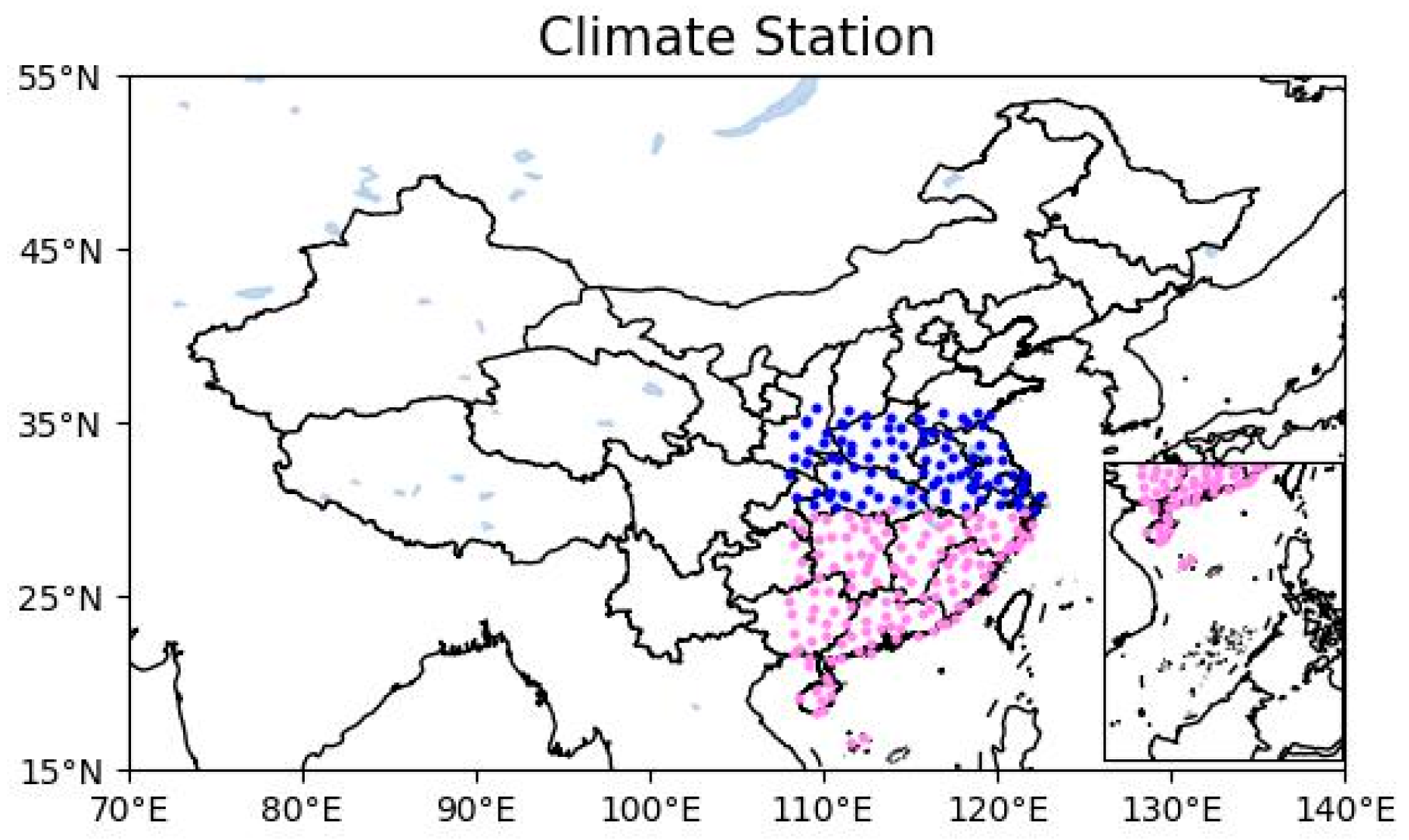
2.1. Materials

In this paper, winter refers to October to March; for example, the winter in 1995/1996 is denoted as 1995/1996. The JRA55 reanalysis data of the Japan Meteorological Agency were used. These data are global daily average grid data with a horizontal resolution of 1.25° × 1.25° and a temporal range of 1960/1961–2019/2020. The sea-level pressure field, 850 hPa zonal wind field, and meridional wind field were selected. Other meteorological datasets included NOAA’s OLR data with a range of 1979/1980–2019/2020 and the daily dataset of meteorological elements of national ground weather stations from 1960/1961 to 2019/2020 in southern China (latitude below 36° N and longitude below 108° E) (Figure 1). Following Chen et al. [21], the research area was divided into an area north of the Yangtze River (blue dots in Figure 1) and another south of the Yangtze River (pink dots in Figure 1), with a dividing line at 30° N. Since the OLR data started in 1979, our prediction test was conducted for the data within the range of 1979/1980–2019/2020. First, 10 years out of 31 years (1979/1980–2009/2010) were randomly selected as the validation set, the remaining 21 years represented the training set, and 2010/2011–2019/2020 was the test set (1670 d).

2.2. Methods

The RPECEs were extracted as follows. First, the extreme threshold was determined. We selected the 10th percentile of the lowest temperatures for each day within a 10 d window (5 before and after) from 1960/1961 to 2019/2020, resulting in 682 d (62 years × 11 d). The criteria for stations with persistent low-temperature events were as follows: the lowest temperature remained below the extreme threshold continuously for 5 d, and the temperature drop during this period exceeded 5 °C [22]. The following conditions had to be met for RPECEs: (1) The 10 neighboring stations of 1 station recorded persistent low-temperature events for at least 5 d. (2) The number of stations meeting condition 1 exceeded 20 on at least one day during this period [21].
We used empirical orthogonal function decomposition (EOF), a CNN, a fully connected neural network (FCNN), Butterworth bandpass filtering, and Morlet wavelet analysis (wavelet analysis) [23].
EOF maximizes the concentration of most spatiotemporal variables based on the principal components of a few independent variables. It extracts the main spatial modes and their time coefficients. In this study, the EOF decomposition of the low-frequency oscillation component of the 2 m minimum temperature in the training set was conducted from 1979 to 2020 to obtain the first spatial mode, which was used as the main feature to characterize the minimum temperature oscillation in the winter. A projection formula was used to project the test set onto the first spatial mode to obtain the time coefficient. The reason was to prevent using information from the test set in the training set.
We employed two signal processing methods. The first one was the Butterworth bandpass filter, which separates the climate cycle components from the observation sequences of stations or grid points. The upper and lower cut-off angle frequencies of the bandpass were used to separate the climate signal in a specific frequency interval from the original signal. The second method was wavelet analysis, which utilizes a convolution kernel to transform the time domain signal of the time series x(t) into the frequency domain ω to decompose the x corresponding to t at different times, obtaining the signal to be analyzed. Morlet wavelet analysis was used to transform the minimum temperature time series data to obtain the wavelet power spectrum corresponding to the period and time in order to determine the statistically significant low-frequency change period.
An FCNN uses a fully connected layer to integrate the inputs from different dimensions; however, it has shortcomings. First, when the data have high dimensionality, the computational efficiency of the FCNN is relatively low. Second, the direct processing of two-dimensional data by the FCNN results in information loss. The CNN was first proposed in 1980 [24]. Due to its structural characteristics, such as local area connection, weight sharing, and downsampling, it is highly suitable for signal processing and extraction from 2D/3D data; and for grid data analysis, such as reanalysis data and modeling. In this study, a CNN was used to extract large-scale signal information (42.5°–150° E, 0°–67.5° N) from the 850 hPa, 500 hPa geopotential height field, and OLR field. The extracted features were used to train the FCNN to predict low-frequency oscillation components.

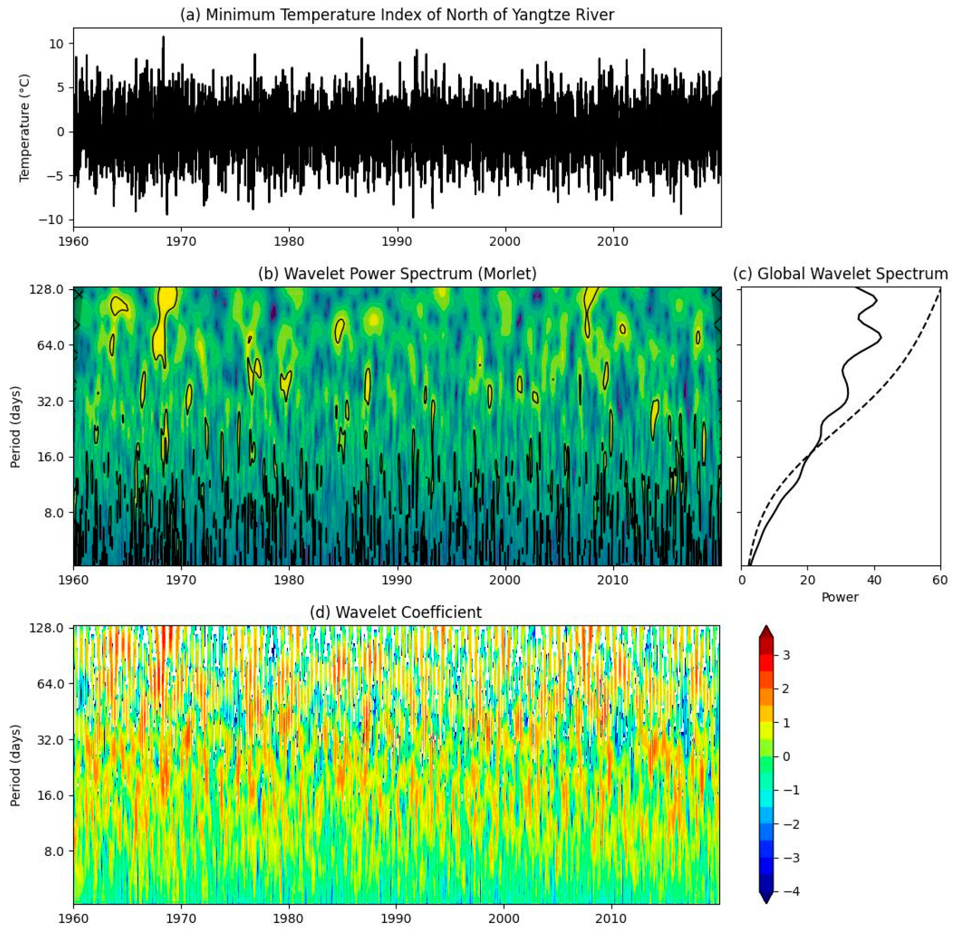
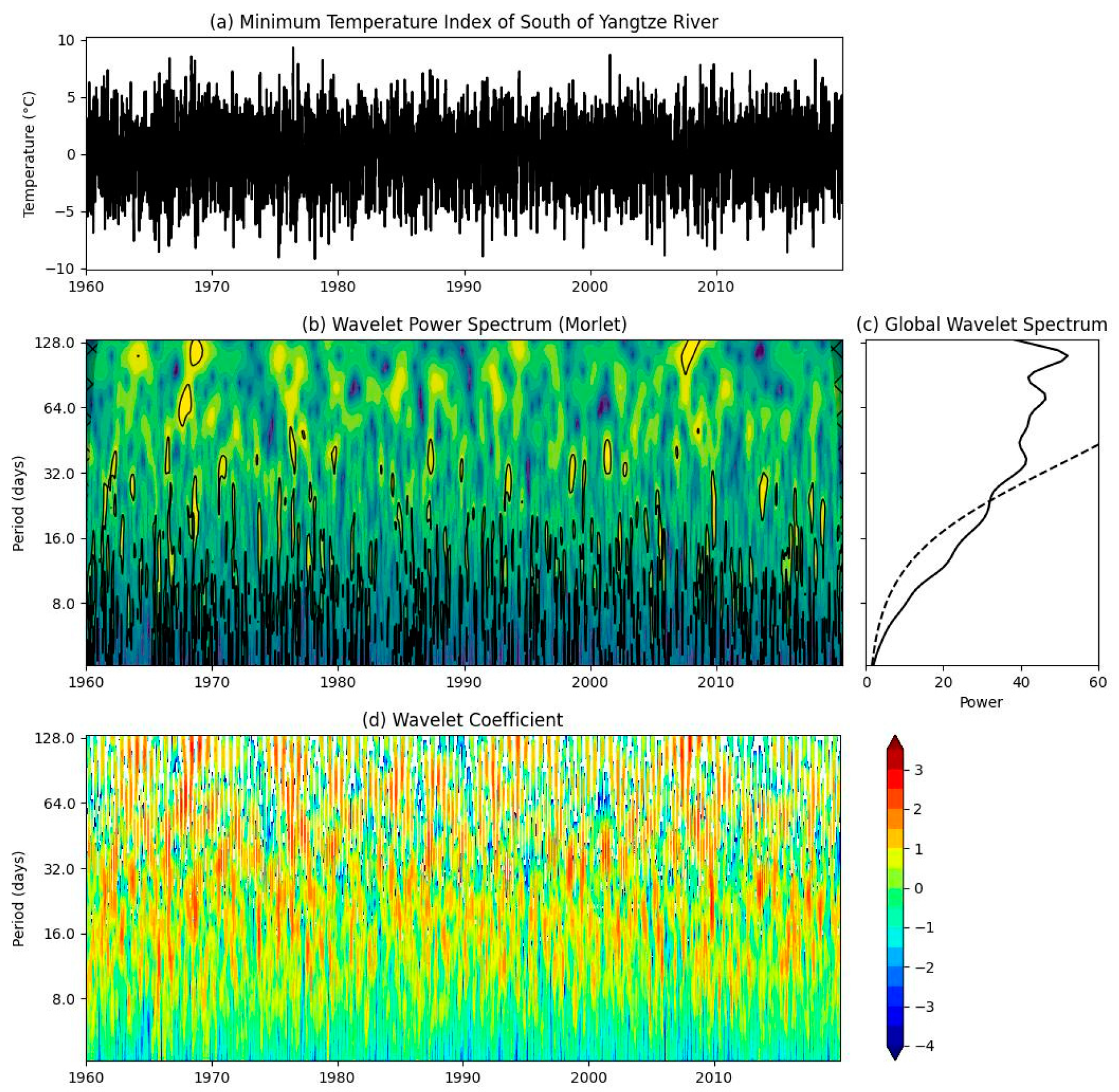
3. Signal Processing of Intraseasonal Oscillation and RPECEs

According to the definition of RPECEs in this paper, we sorted the data by the start and end dates and obtained the duration (days) and peak dates of RPECEs in Table 1. We analyzed the 850 hPa temperature field, 500 hPa geopotential height field, 850 hPa wind field, and sea-level pressure field. As shown in Figure 2, the low-level warm anomaly in Siberia corresponds to the positive geopotential anomaly in the middle and upper atmosphere, and the low-level cold anomaly in southern China corresponds to the negative geopotential anomaly in the middle and upper atmosphere. The result shows that we can use the geopotential height at 500 hPa in the middle layer and the geopotential height at 200 hPa in the upper layer to indicate changes in the atmospheric temperature in the lower layer. Figure 3 shows that the extremely low temperatures in southern China were caused by the significant northerly wind component extending southward to southern China via an anticyclone.
After removing the annual cycle and annual average from the daily minimum temperature series from 1960 to 2020, Morlet wavelet analysis was performed. Figure 4b and Figure 5b show the wavelet power spectra. The spectral values passing the 0.05 significance level are surrounded by thick solid lines, indicating that the period is significant. Figure 4c and Figure 5c show the global wavelet power spectrum. The dotted line represents the critical value of the 0.05 significance level in the cycle. The spectral value on the right side of the dotted line indicates a 0.05 significance level. Figure 4 shows a low-frequency change period of about 20 d in the low-temperature events in the northern Yangtze River region, and Figure 5 indicates a low-frequency change period of about 30 d in the southern Yangtze River region. Both exhibit quasi-biweekly variations of 10–20 d and atmospheric intraseasonal oscillations of 30–60 d. The work of Zhu [25] confirmed this result, indicating that the minimum temperature in winter has low-frequency characteristics.
After removing the annual cycle and annual average from the daily minimum temperature series from 1995 to 2020, the Butterworth filtering of the low-frequency oscillation series was conducted after station-by-station filtering for 10–20 d and 30–60 d. EOF decomposition was performed on the low-frequency oscillation series at multiple stations. As shown in Figure 6, the explained variances of the first mode of the minimum temperature on the two time scales (10–20 d and 30–60 d) for the northern Yangtze River region were 78.9% and 80%, respectively. The physical meaning of the first mode is that the northern region experienced uniform cold conditions. The time coefficient represents the degree of coldness, and the higher the positive phase, the greater the degree of coldness in this region. Similarly, Figure 7 shows the explained variance for the southern Yangtze River region (79%). The time coefficient indicates uniform coldness.
We calculated the proportion of the 46 RPECEs occurring since 1979 in the phases of the low-frequency components, and their time coefficient amplitude was higher than one standard deviation. The proportion was 90% in the northern Yangtze River region and 80% in the southern Yangtze River region, indicating that most RPECEs were strongly correlated with low-frequency oscillations. Thus, we can predict the occurrence of RPECE events by predicting the time coefficient of low-frequency oscillations. The standard deviation of the positive phase of the time coefficient of the low-frequency oscillation was calculated. If the time coefficient of the low-frequency oscillation was higher than the positive phase of one standard deviation in a certain period, it was highly likely that it was a low-frequency oscillation of RPECEs. Our goal was to predict the time coefficient of low-frequency oscillations. However, it is worth noting that not every high positive phase indicates a large-scale low-temperature event.

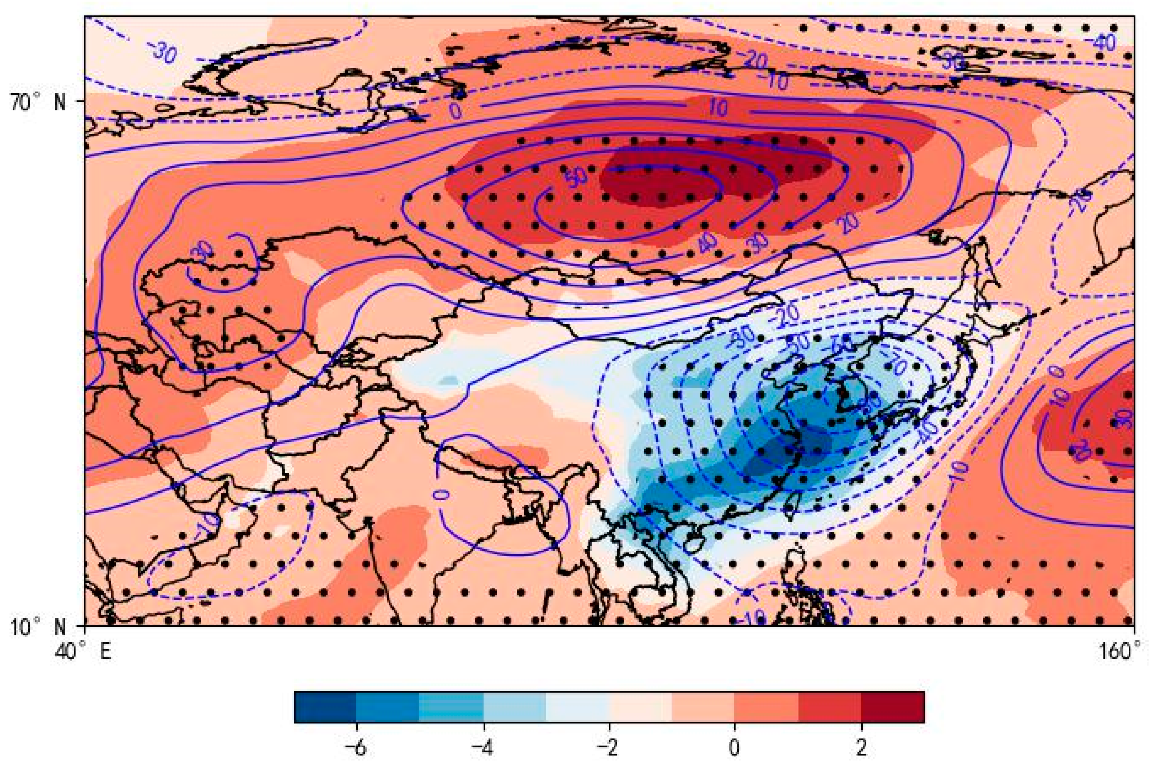
4. Extended-Range Forecast

The CNN deep learning method commonly used in climate prediction [26,27] was used to obtain an extended-range forecast of RPECEs. Specifically, we predicted the time coefficient of low-frequency oscillations.

4.1. Deep Learning Model for Extended-Range Forecast

The CNN was used to determine the spatial-temporal characteristics of the low-frequency field and the OLR field in the current time (t) and the previous time (t-25 d, t-20 d, t-15 d, t-10 d, and t-5 d). The correlation between the feature set of large-scale circulation factors and the time coefficient of the low-frequency oscillation component of the minimum air temperature was calculated. The structure of the CNN model is shown in Figure 8. It has three convolutional layers, two pooling layers, and one fully connected layer. The convolution operation extracts features from the two-dimensional longitude and latitude data, and the pooling operation reduces the feature dimensions of adjacent data at certain locations. The fully connected layer improves the nonlinear fitting performance of the CNN by stacking multiple neurons.
The first layer (18) represents 18 channels, i.e., 6 times H200, H500, and OLR, and the two-dimensional vector of each channel is 28×44, because the spatial range of each element is (0°–67.5° N, 42.5°–150° E), and the spatial resolution is 2.5° × 2.5°. The output is 1 × 1, which is the time coefficient of the low-frequency oscillation component of the minimum temperature. It is predicted for the following 15 d.
The convolution kernel size during network training was 3 × 3, and the size of the pooling kernel was 2 × 2. Maximum pooling was adopted; the learning rate was 0.005, the sample batch size was 32, and the loss function was l 1 -loss. The ReLU activation function and Kaiming initialization were used. A dropout layer was inserted before the fully connected layer to prevent overfitting. The features extracted by the CNN were discarded or kept based on their probability.

4.2. Model Validation

We used the 2010/2011–2019/2020 dataset for model validation. Four RPECEs occurred during the test period: 28 October to 2 November in 2010, 10 February to 15 February in 2014, 23 January to 27 January in 2016, and 25 January to 30 January in 2018.
As shown in Figure 9, three of the four events were correctly predicted. Similar trends were observed for the predicted and observed values. The prediction for the period in Figure 9a exhibits a phase deviation. Two criteria were used to assess the prediction accuracy:
P O D = N A N A + N C F A R = N B N A + N B
where NA represents hits, NB represents false alarms, and NC represents misses. POD denotes the probability of detection, and FAR is the false alarm rate. POD is 0.75, and FAR is 0.76. A positive phase higher than one standard deviation corresponds to low-frequency oscillation. The average correlation coefficient between the observed and predicted low-frequency oscillation component for the test set is 0.41 for the deep learning method and 0.1 for the linear method.
We conducted another numerical experiment using test data in the range of 1979/1980–1988/1989; 10 years out of 31 years (1989/1990–2009/2010) were randomly selected as the validation set, and the remaining 21 years were used as the training set. Previous periods (1979/1980–1988/1989) had more extreme cold events. We obtained predictions for 15 RPECEs. POD is 0.6, and FAR is 0.55. POD and FAR are lower than those in the previous experiment. The results indicate that the model has a reasonable predictive ability for the low-frequency oscillation time coefficient in this period and can describe the trend of the low-frequency oscillation curve.

5. Conclusions

The innovation of this article lies in the following points:
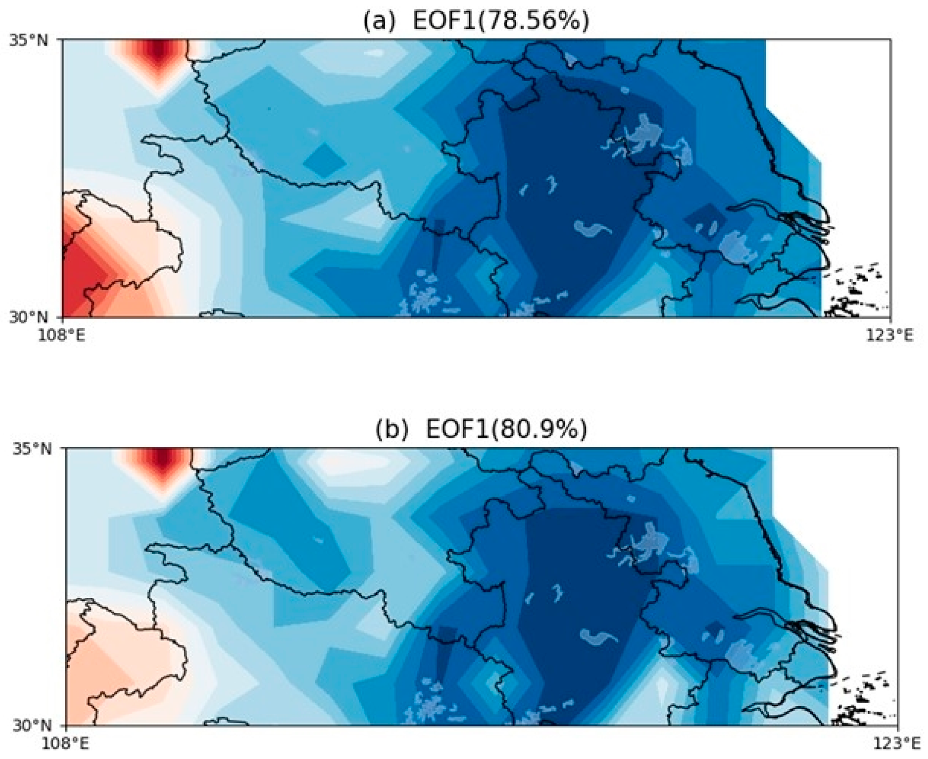
  • The minimum temperature in winter exhibited low-frequency oscillations. Morlet wavelet analysis indicated two low-frequency oscillation periods of 10–20 d and 30–60 d. EOF decomposition showed that the oscillation period had a high explained variance for the first mode, indicating uniform coldness in the study area. This result can be used to perform extended-range forecasts.
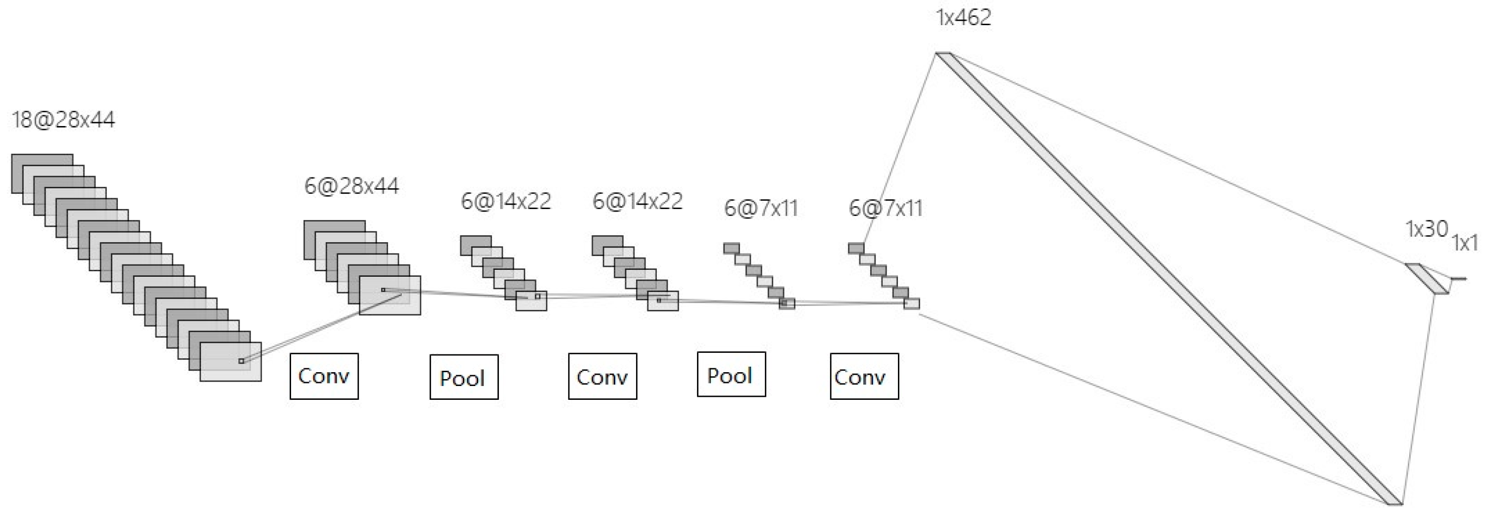
  • A CNN deep learning model was established, and the geopotential height of the reanalysis data field and OLR data were used. The correlation between the large-scale circulation factor feature set and the time coefficient of the low-frequency oscillation of the minimum temperature was calculated.
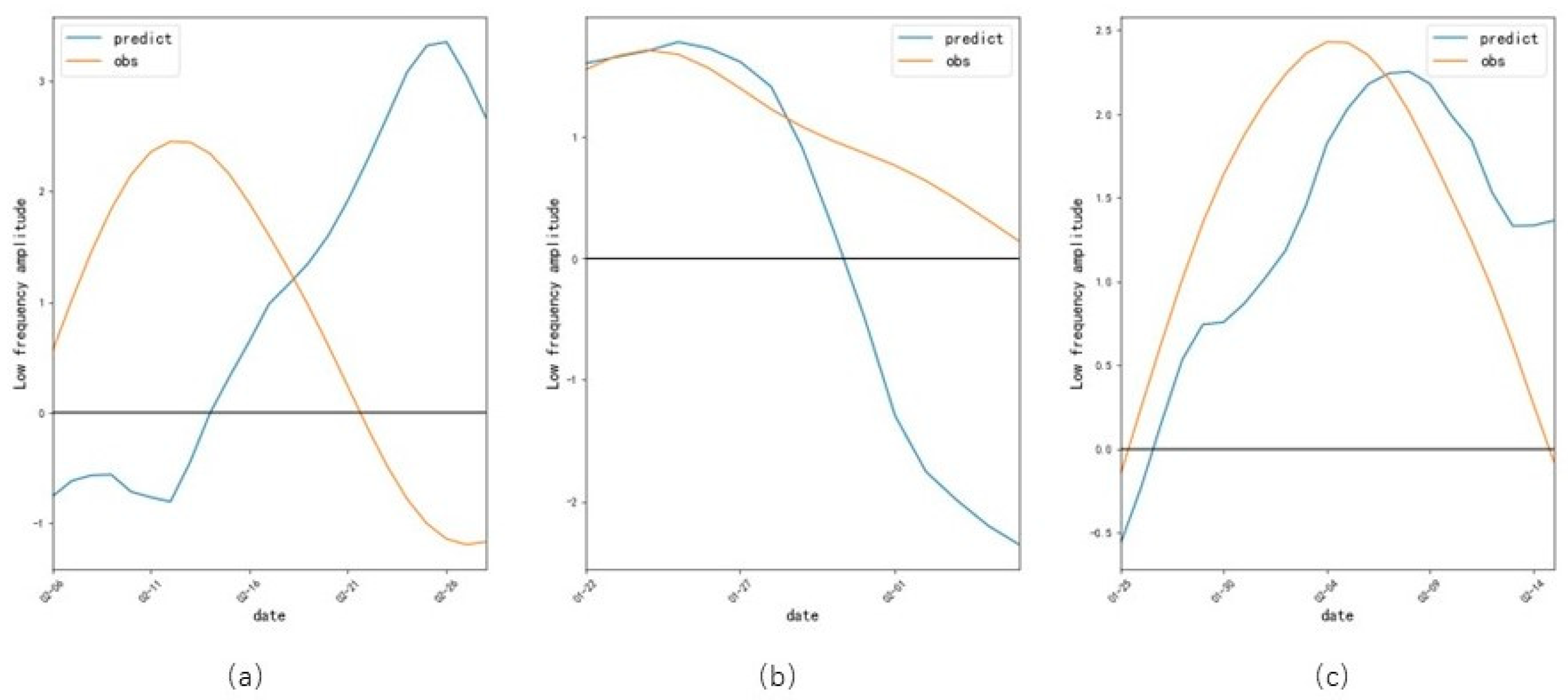
  • The proposed model reflects the state of the atmospheric low-frequency oscillation curve, enabling the prediction of RPECEs.
Several aspects of the model require improvement. (1) The high FAR must be lowered. (2) Non-bandpass filtering could be used to obtain low-frequency components in real time. (3) More advanced neural network models could be used, such as the sequential neural network model RNN. (4) RPECEs and low-frequency oscillations do not occur often; therefore, other conditions should be used to indicate the occurrence of RPECEs.

Author Contributions

All authors contributed to this manuscript. Conceptualization, F.W.; methodology, F.W. and W.W.; software, W.W. and X.Y.; validation, F.W. and B.L.; formal analysis, W.W., F.W. and B.L.; investigation, W.W. and F.W.; resources, W.W.; data curation, W.W.; writing—original draft preparation, W.W.; writing—review and editing, Y.W. and B.L; visualization, W.W.; supervision, Y.W. and F.W.; project administration, Y.W.; funding acquisition, Y.W. All authors have read and agreed to the published version of the manuscript.

Funding

This research was funded by grants from the National Key Research and Development Program (2022YFC3003903) and the CAMS project (2023Z013, 2023Z022).

Institutional Review Board Statement

Not applicable.

Informed Consent Statement

Not applicable.

Data Availability Statement

The JRA reanalysis data are available from (https://data.diasjp.net/dl/storages/filelist/dataset:204, accessed on 16 August 2023). The NOAA’s OLR data are available from (https://www.ncei.noaa.gov/products/climate-data-records/outgoing-longwave-radiation-daily, accessed on 16 August 2023). The daily dataset of meteorological elements of national ground weather stations are not available due to restrictions privacy.

Conflicts of Interest

The authors declare no conflict of interest.

References

  1. Tao, S. Study on East Asian cold waves in China during recent 10 years. Acta Meteorol. Sin. 1959, 30, 226–230. [Google Scholar]
  2. Ding, Y. The propagation of the winter monsoon during cold air outbreaks in east Asia and the associated planetary-scale effect. J. Appl. Meteorol. Climatol. 1991, 2, 124–132. [Google Scholar]
  3. Qian, W.; Zhang, W. Changes in Cold Wave Events and Warm Winter in China during the Last 46 Years. Chin. J. Atmos. Sci. 2007, 31, 1266–1278. [Google Scholar]
  4. Wei, F. Probability Distribution of Minimum Temperature in Winter Half Years in China. Clim. Chang. Res. 2008, 4, 8–11. [Google Scholar]
  5. Bueh, C. Research on Persistent Extreme Cold Events in China; China Meteorological Press: Beijing, China, 2015. [Google Scholar]
  6. Shi, N.; Bueh, C. A Specific Stratospheric Precursory Signal for the Extensive and Persistent Extreme Cold Events in China. Chin. J. Atmos. Sci. 2015, 39, 210–220. [Google Scholar]
  7. Bueh, C.; Fu, X.Y.; Xie, Z.W. Large-scale circulation features typical of wintertime extensive and persistent low temperature events in China. Atmos. Ocean. Sci. Lett. 2011, 4, 235–241. [Google Scholar]
  8. Zhang, Z.; Qian, W. Precursors of Regional Prolonged Low Temperature Events in China during Winter Half Year. Chin. J. Atmos. Sci. 2012, 36, 1269–1279. [Google Scholar]
  9. Yang, Q.M. A study of the extended-range forecast for the low frequency temperature and high temperature weather over the lower reaches of Yangtze River Valley in summer. Adv. Earth Sci. 2018, 33, 385–395. [Google Scholar]
  10. Yang, Q.M. Extended-range forecast for the low-frequency oscillation of temperature and low-temperature weather over the lower reaches of the Yangtze River in winter. Chin. J. Atmos. Sci. 2021, 45, 21–36. [Google Scholar]
  11. Hsu, P.C.; Li, T.; You, L.; Gao, J.; Ren, H.L. A spatial–temporal projection model for 10–30 day rainfall forecast in South China. Clim. Dyn. 2015, 44, 1227–1244. [Google Scholar] [CrossRef]
  12. Hsu, P.C.; Zang, Y.X.; Zhu, Z.W.; Li, T. Subseasonal-to-seasonal (S2S) prediction using the spatial-temporal projection model (STPM). Trans. Atmos. Sci. 2020, 43, 212–224. [Google Scholar]
  13. Zhu, Z.W.; Li, T. Statistical extended-range forecast of winter surface air temperature and extremely cold days over China. Q. J. R. Meteorol. Soc. 2017, 143, 1528–1538. [Google Scholar] [CrossRef]
  14. Lee, S.; Moon, J.; Wang, B.; Kim, H. Subseasonal Prediction of Extreme Precipitation over Asia: Boreal Summer Intraseasonal Oscillation Perspective. J. Clim. 2017, 30, 2849–2865. [Google Scholar] [CrossRef]
  15. Lei, L.; Hsu, P.C.; Gao, Q.J.; Xie, H.J. Extended-range forecasting method of summer daily maximum temperature in the Yangtze River Basin based on convolutional neural network. Trans. Atmos. Sci. 2022, 45, 835–849. [Google Scholar]
  16. Wu, J.; Ren, H.L.; Zhang, P.; Wang, Y.; Liu, Y.; Zhao, C.; Li, Q. The dynamical-statistical subseasonal prediction of precipitation over China based on the BCC new-generation coupled model. Clim. Dyn. 2022, 59, 1213–1232. [Google Scholar] [CrossRef]
  17. Zhang, K.Y.; Li, J.; Hsu, P.C.; Zhu, Z.W. The dynamical-statistical extended-range prediction of precipitation and extreme precipitation events over southern China. Acta Meteorol. Sin. 2023, 81, 79–93. [Google Scholar]
  18. Kim, M.; Yoo, C.; Choi, J. Enhancing subseasonal temperature prediction by bridging a statistical model with dynamical Arctic Oscillation forecasting. Geophys. Res. Lett. 2021, 48, e2021GL093447. [Google Scholar] [CrossRef]
  19. Qian, Y.; Hsu, P.-C.; Murakami, H.; Xiang, B.; You, L. A hybrid dynamical-statistical model for advancing subseasonal tropical cyclone prediction over the western North Pacific. Geophys. Res. Lett. 2020, 47, e2020GL090095. [Google Scholar] [CrossRef]
  20. Zhang, D.Q.; Zheng, Z.H.; Chen, L.J.; Zhang, P.Q. Advances on the predictability and prediction methods of 10–30 d extended range forecast. J. Appl. Meteorol. Sci. 2019, 30, 416–430. [Google Scholar]
  21. Chen, G.J.; Wei, F.Y.; Yao, W.Q.; Zhou, X. Extended range forecast experiments of persistent winter low temperature indexes based on intra-seasonal oscillation over southern China. Acta Meteorol. Sin. 2017, 75, 400–414. [Google Scholar]
  22. Zhang, Z.J.; Qian, W.H. Identifying regional prolonged low temperature events in China. Adv. Atmos. Sci. 2011, 28, 338–351. [Google Scholar] [CrossRef]
  23. Torrence, C.; Compo, G.P. A practical guide to wavelet analysis. Bull. Am. Meteorol. Soc. 1998, 79, 61–78. [Google Scholar] [CrossRef]
  24. Fukushima, K. Neocognitron: A self organizing neural network model for a mechanism of pattern recognition unaffected by shift in position. Biol. Cybern. 1980, 36, 193–202. [Google Scholar] [CrossRef]
  25. Zhu, Y.Y.; Jiang, J. The intraseasonal characteristics of wintertime persistent cold anomaly in China and the role of low frequency oscillation in the low latitude and midlatitude. J. Trop. Meteorol. 2013, 29, 649–655. [Google Scholar]
  26. Ham, Y.G.; Kim, J.H.; Luo, J.J. Deep learning for multi-year ENSO forecasts. Nature 2019, 573, 568–572. [Google Scholar] [CrossRef]
  27. He, S.P.; Wang, H.J.; Li, H.; Zhao, J.Z. Machine learning and its potential application to climate prediction. Trans. Atmos. Sci. 2021, 44, 26–38. [Google Scholar]
Figure 1. Map of weather stations in southern China.
Atmosphere 14 01572 g001
Figure 2. Composite of temperature anomalies in 850 hPa (colors, unit: °C) and geopotential height anomalies in the 500 hPa (contours, unit: gpm) of RPECEs (the dots indicate that the relationship does not exceed the 0.05 significance level).
Atmosphere 14 01572 g002
Figure 3. Composite of wind anomalies in 850 hPa (vectors, unit: m/s) and sea level pressure anomalies (contours, unit: hPa) of RPECEs (the dots indicate that the relationship does not exceed the 0.05 significance level).
Atmosphere 14 01572 g003
Figure 4. Minimum temperature index (a), Morlet wavelet power spectrum (b), global wavelet spectrum (c), and wavelet coefficient (d) from 1960 to 2020 in the northern Yangtze River region.
Atmosphere 14 01572 g004
Figure 5. Minimum temperature index (a), Morlet wavelet power spectrum (b), global wavelet spectrum (c), and wavelet coefficient (d) from 1960 to 2020 in the southern Yangtze River region.
Atmosphere 14 01572 g005
Figure 6. The explained variance of the first mode of the minimum temperature in the northern Yangtze River region for (a) 10–20 days and (b) 30–60 days.
Atmosphere 14 01572 g006
Figure 7. The same as Figure 6 but for the southern Yangtze River region.
Atmosphere 14 01572 g007
Figure 8. Convolutional neural network to predict the principal components of low-frequency oscillations (Conv: convolution; Pool: pooling).
Atmosphere 14 01572 g008
Figure 9. Predicted and observed RPECEs: (a) 10 February 2014–15 February 2014 (30–60 d), (b) 23 January 2016–27 January 2016 (30–60 d), and (c) 25 January 2018–30 January 2018 (30–60 d).
Atmosphere 14 01572 g009
Table 1. The start and end dates, durations, and peak dates of the RPECEs.
NumberStart and End DateDurationPeak
13 October 1979–15 October1310 October 1979
25 February 1980–11 February77 February 1980
322 October 1981–26 October523 October 1981
46 November 1981–10 November58 November 1981
524 March 1982–28 March525 March 1982
621 January 1983–25 January523 January 1983
727 November 1983–2 December61 December 1983
818 January 1984–22 January522 January 1984
919 December 1984–29 December1124 December 1984
1011 March 1985–16 March612 March 1985
112 October 1985–6 October53 October 1985
127 December 1985–12 December611 December 1985
1327 February 1986–3 March52 March 1986
1431 October 1987–4 November53 November 1987
1527 November 1987–2 December630 November 1987
165 December 1987–9 December57 December 1987
171 March 1988–5 March55 March 1988
1829 November 1989–3 December52 December 1989
1912 November 1991–16 November515 November 1991
2026 December 1991–30 December528 December 1991
2117 March 1992–29 March1324 March 1992
224 October 1992–8 October55 October 1992
2316 October 1992–21 October618 October 1992
249 November 1992–14 November610 November 1992
2515 January 1993–25 January1116 January 1993
2628 January 1993–1 February529 January 1993
277 October 1993–12 October68 October 1993
2818 November 1993–24 November721 November 1993
2919 October 1994–26 October823 October 1994
3017 February 1996–24 February820 February 1996
3119 March 1998–23 March521 March 1998
3220 December 1999–25 December623 December 1999
332 November 2000–6 November52 November 2000
3414 November 2001–23 November1016 November 2001
357 October 2002–12 October68 October 2002
362 November 2003–13 November610 November 2003
373 October 2004–7 October54 October 2004
3815 December 2005–19 December515 December 2005
3922 January 2008–2 February1329 January 2008
4010 January 2009–15 January622 January 2009
4111 November 2009–19 November917 November 2009
4216 February 2010–20 February518 February 2010
4328 October 2010–2 November630 October 2010
4410 February 2014–15 February611 February 2014
4523 January 2016–27 January523 January 2016
4625 January 2018–30 January628 January 2018
Disclaimer/Publisher’s Note: The statements, opinions and data contained in all publications are solely those of the individual author(s) and contributor(s) and not of MDPI and/or the editor(s). MDPI and/or the editor(s) disclaim responsibility for any injury to people or property resulting from any ideas, methods, instructions or products referred to in the content.

