
Evaluation of Ten Fresh Snow Density Parameterization Schemes for Simulating Snow Depth and Surface Energy Fluxes on the Eastern Tibetan Plateau


Abstract
1. Introduction
2. Data and Methods
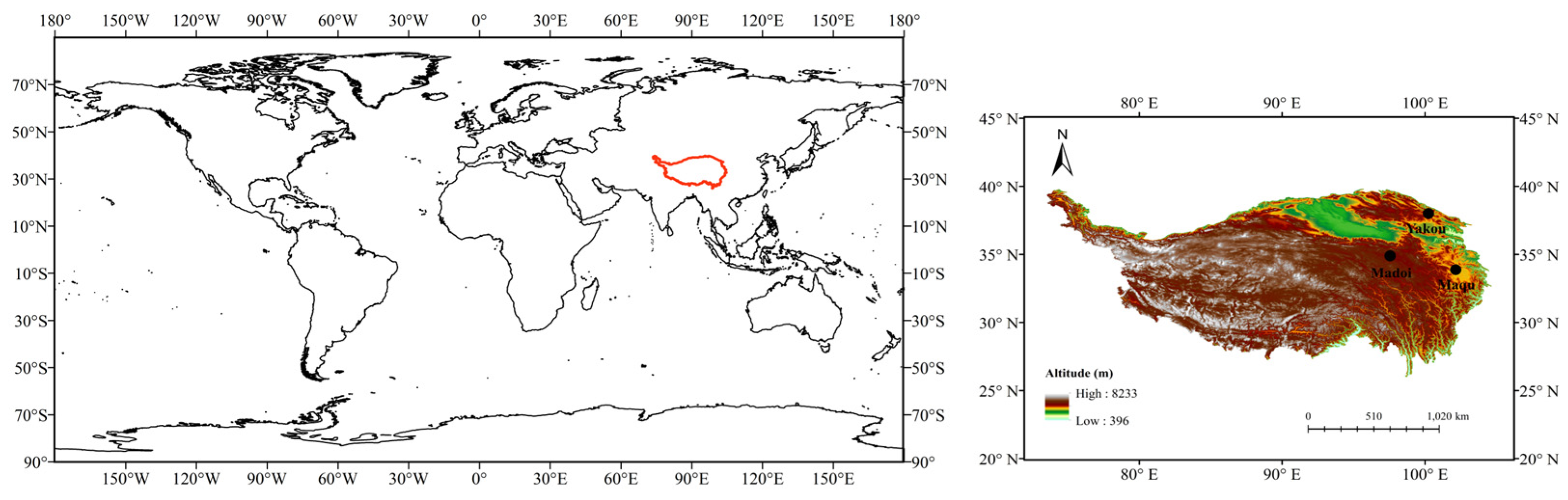
2.1. Study Area
2.2. Data
2.3. Methods
2.3.1. The Representatives of Stations and Snow Processes
2.3.2. Model and Setup
- (1)
- From 1 November 2014 to 20 January 2015, 81 d in total (Period B), among which the spin-up period was 39 d, from 1 November to 9 December, and atmospheric forcing was also updated every 30 min.
- (2)
- From 21 October 2018 to 17 April 2019, a total of 179 d (Period D). The initial soil temperature and humidity settings were added to make the model run stably in this period, due to data limitations caused by spin up (Table S4). Since the simulation starts in October, the initial ice content of the soil is zero.
- (1)
- Another discontinuous snow process in a short period of time, from 11 August 2015 to 30 September 2015, with a spin-up time period from 1 August to 10 August (Period C).
- (2)
- One continuous snow process similar to that at Yakou, from 1 October 2014 to 20 March 2015, with a spin-up time period from 1 August to 30 September (Period E).
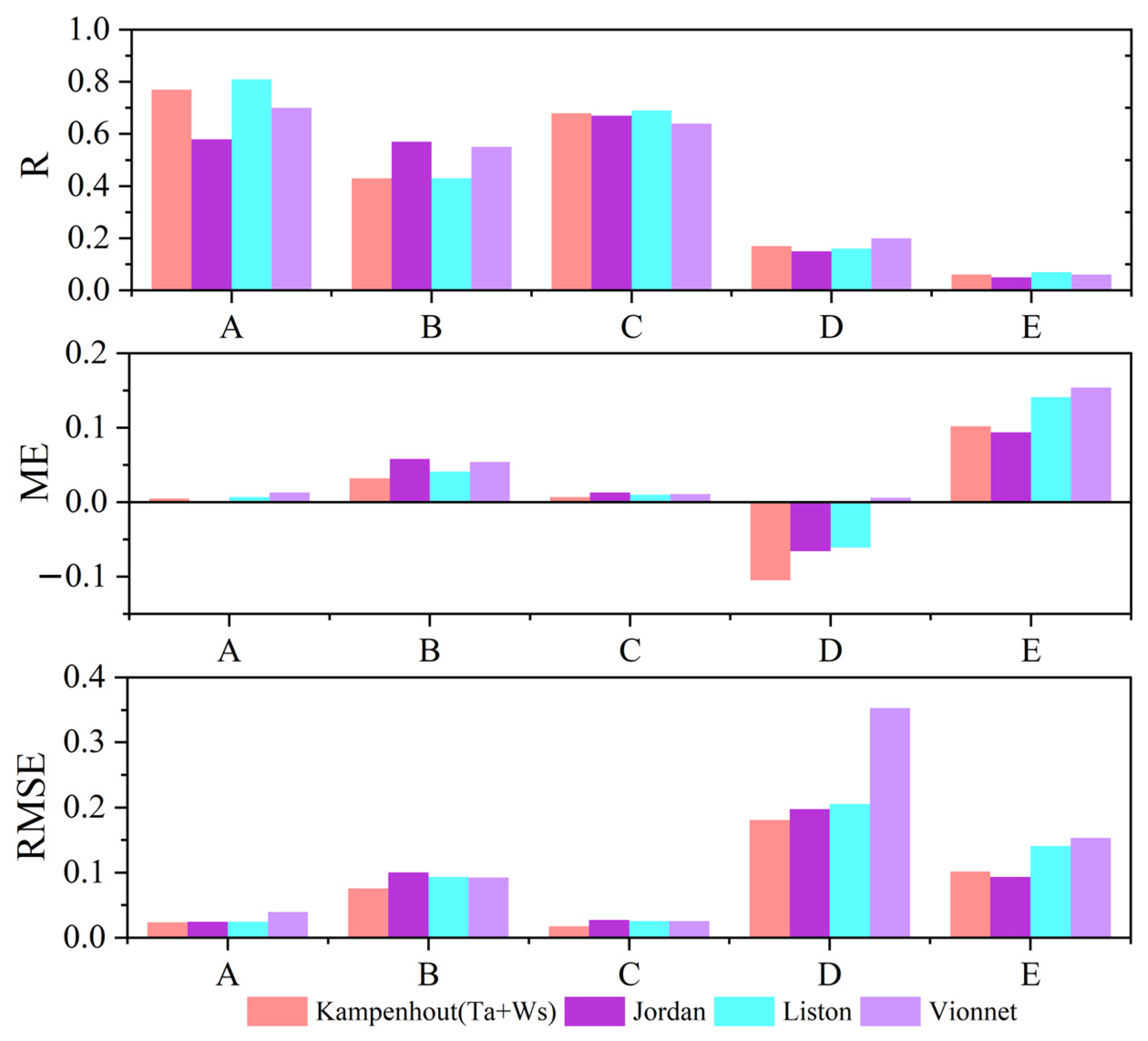
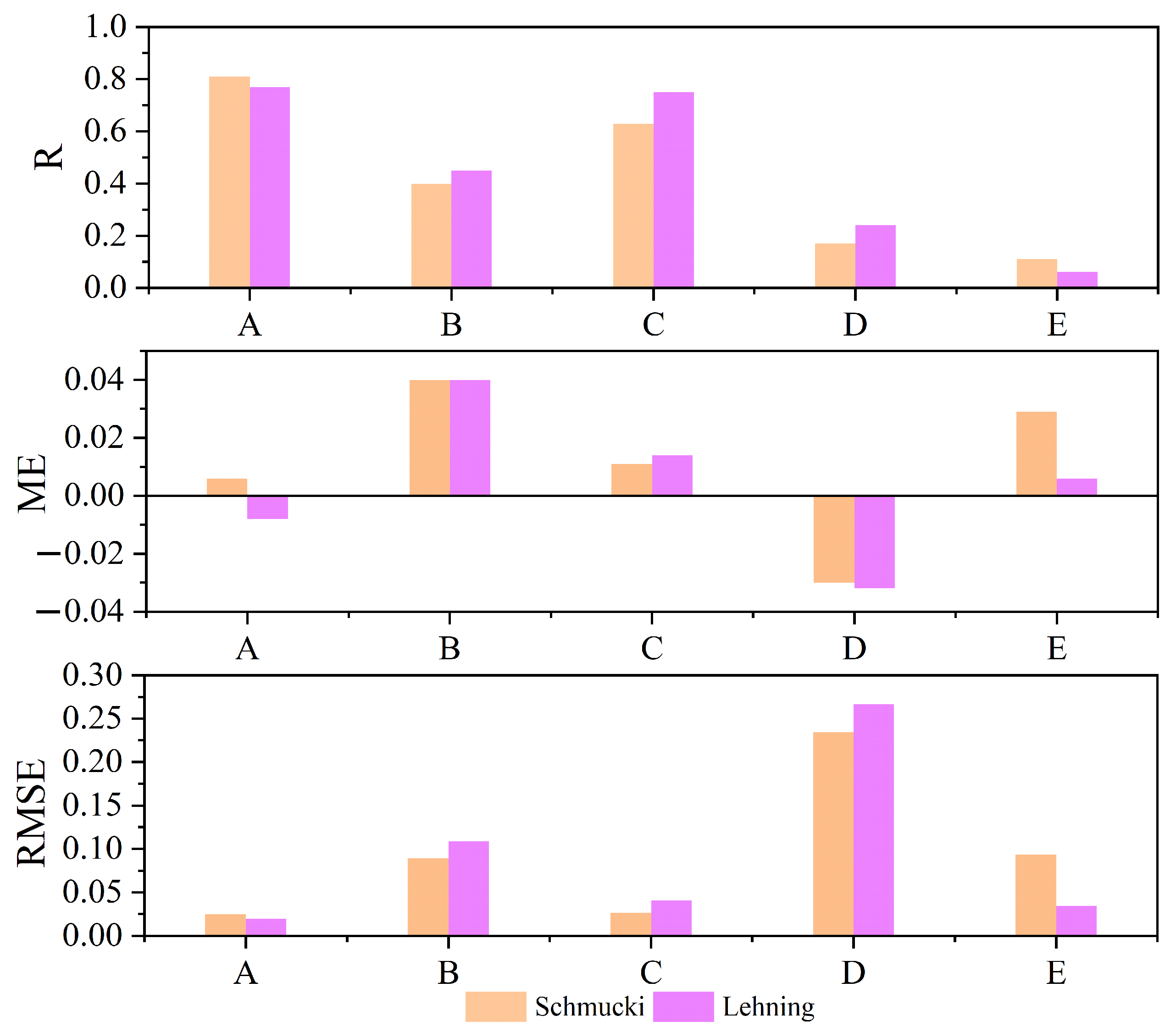
2.3.3. Evaluation Method of Simulation Effects
- (1)
- The correlation coefficient (R): indicates the degree of similarity between the simulated value and the observed value change trend.
- (2)
- Mean deviation (ME): represents the size of the overall deviation between the simulated value and the observed value.
- (3)
- Root mean square error (RMSE): represents the simulated value. The magnitude of the deviation between the value and the observed value is the superposition of the simulation effect of the simulation value at each moment in the entire simulation period.
3. Results
3.1. Simulation of Snow Depth in Schemes
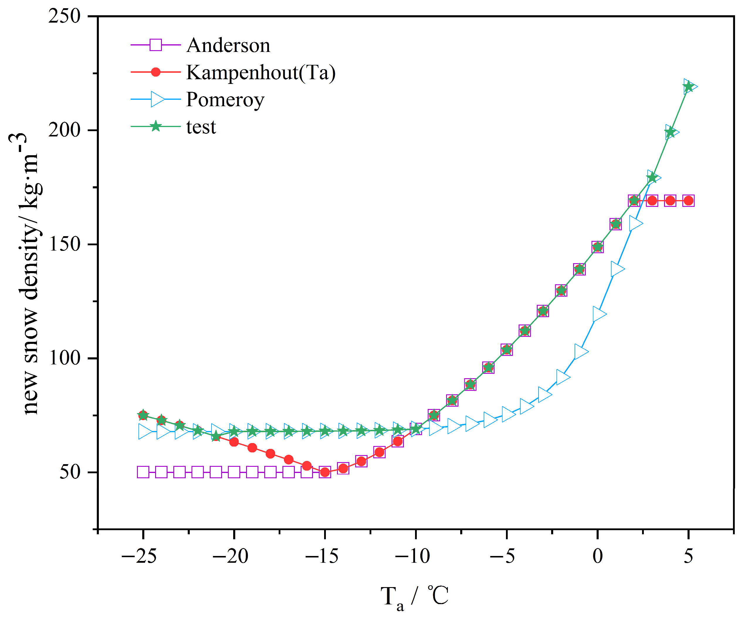
3.1.1. Air Temperature Schemes
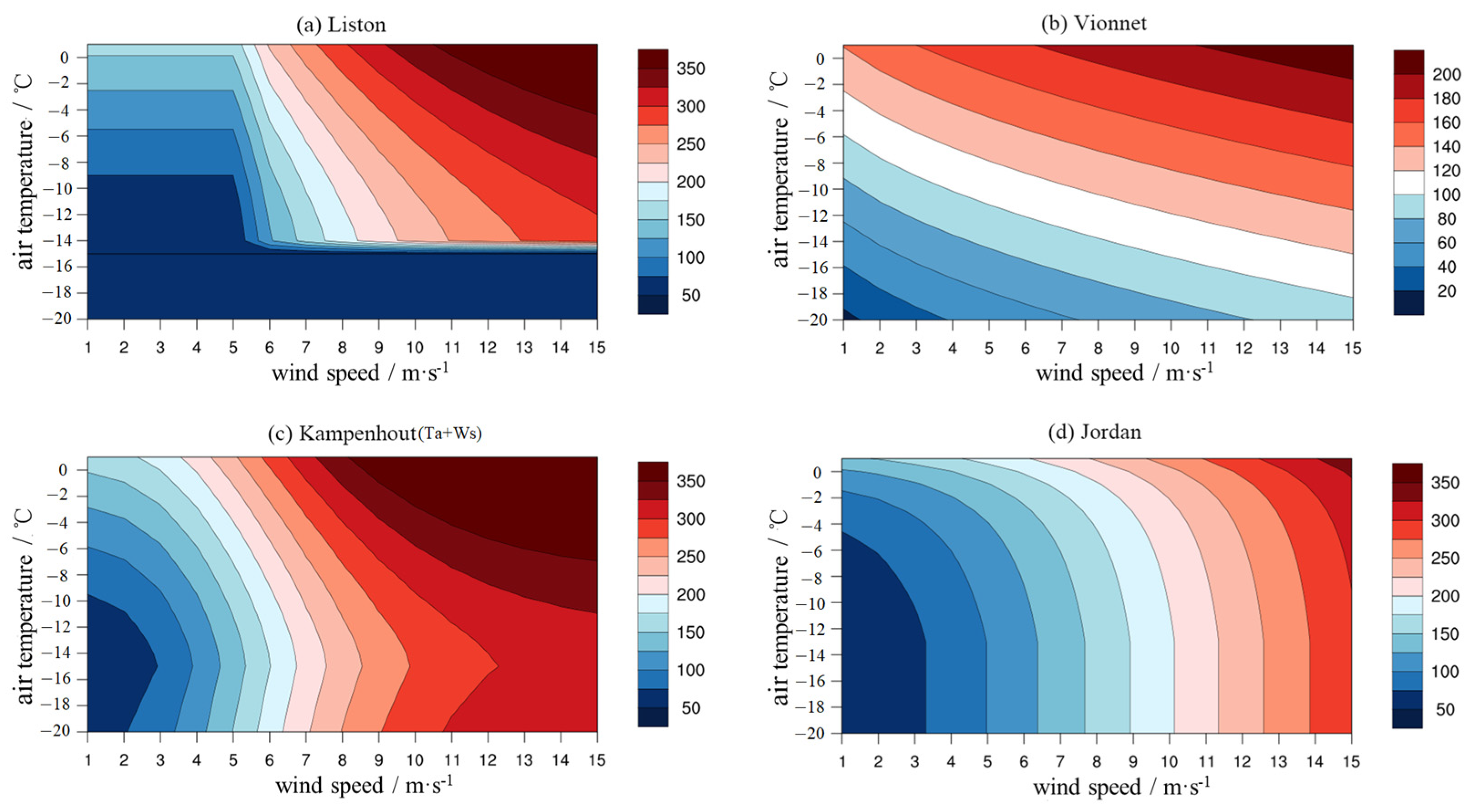
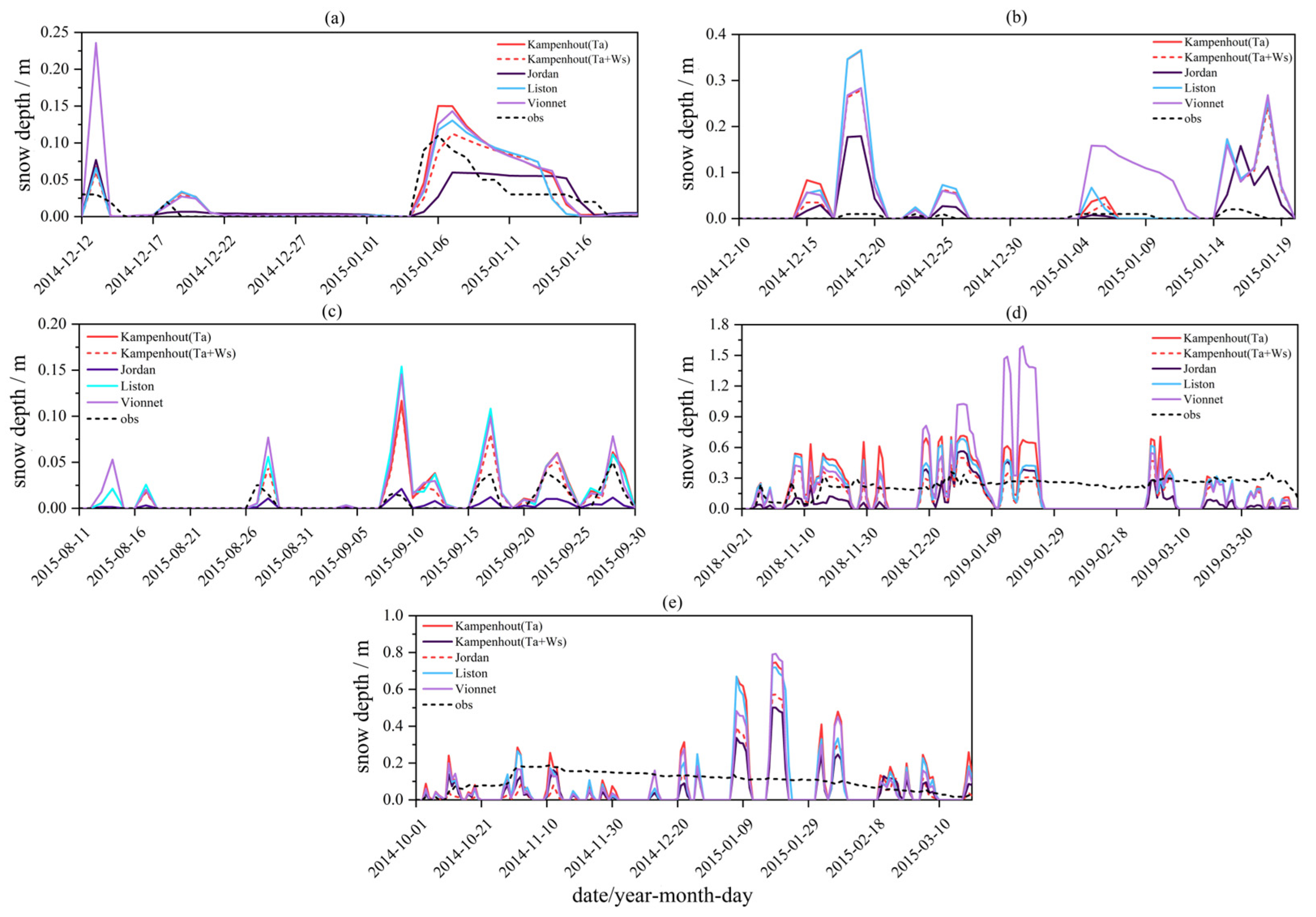
3.1.2. Wind Speed and Air Temperature Schemes
3.1.3. Relativity Humidity, Wind Speed, and Air Temperature Schemes
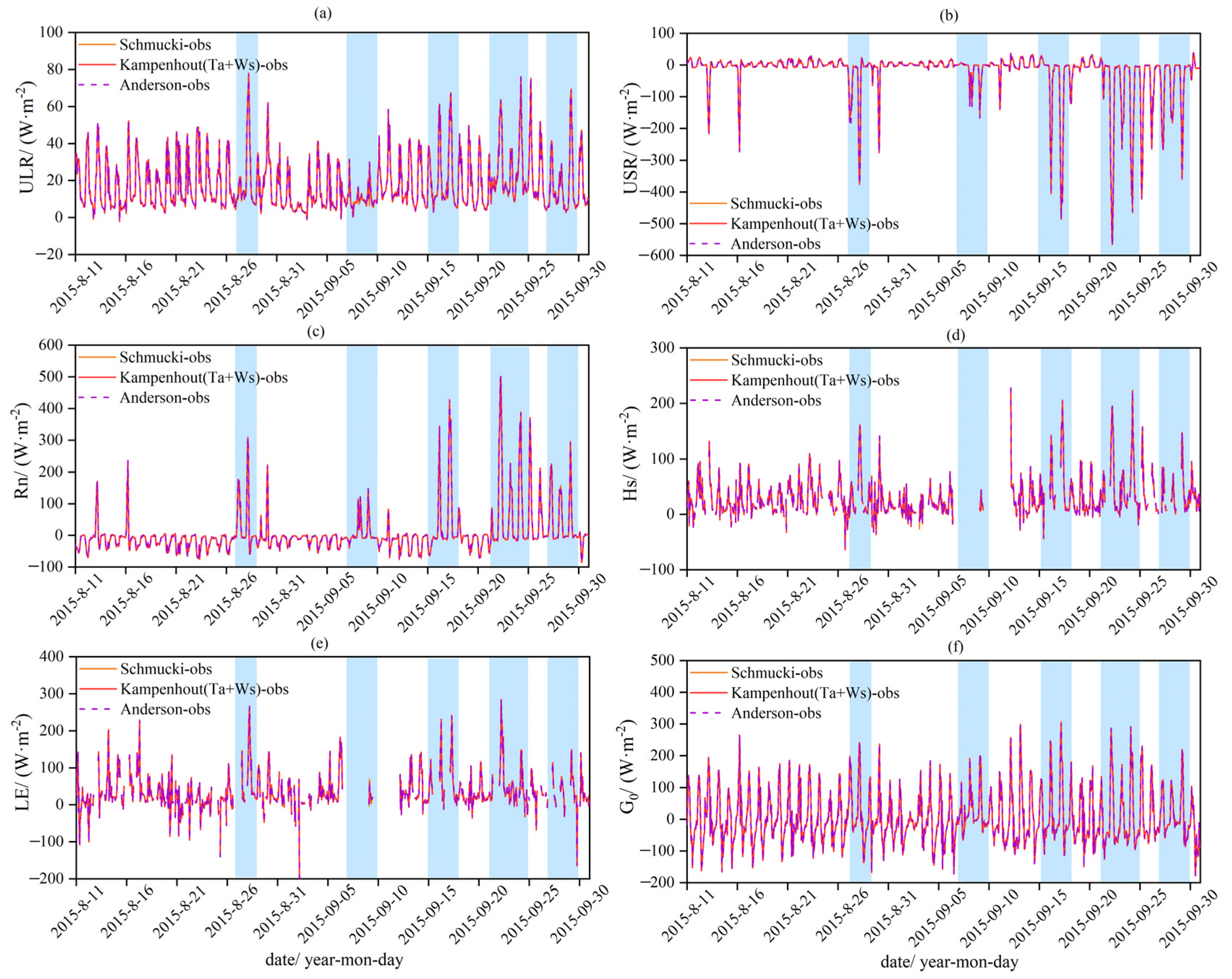
3.2. Improved Radiation and Energy Simulation with Better Fresh Snow Density Schemes
4. Discussion
- (1)
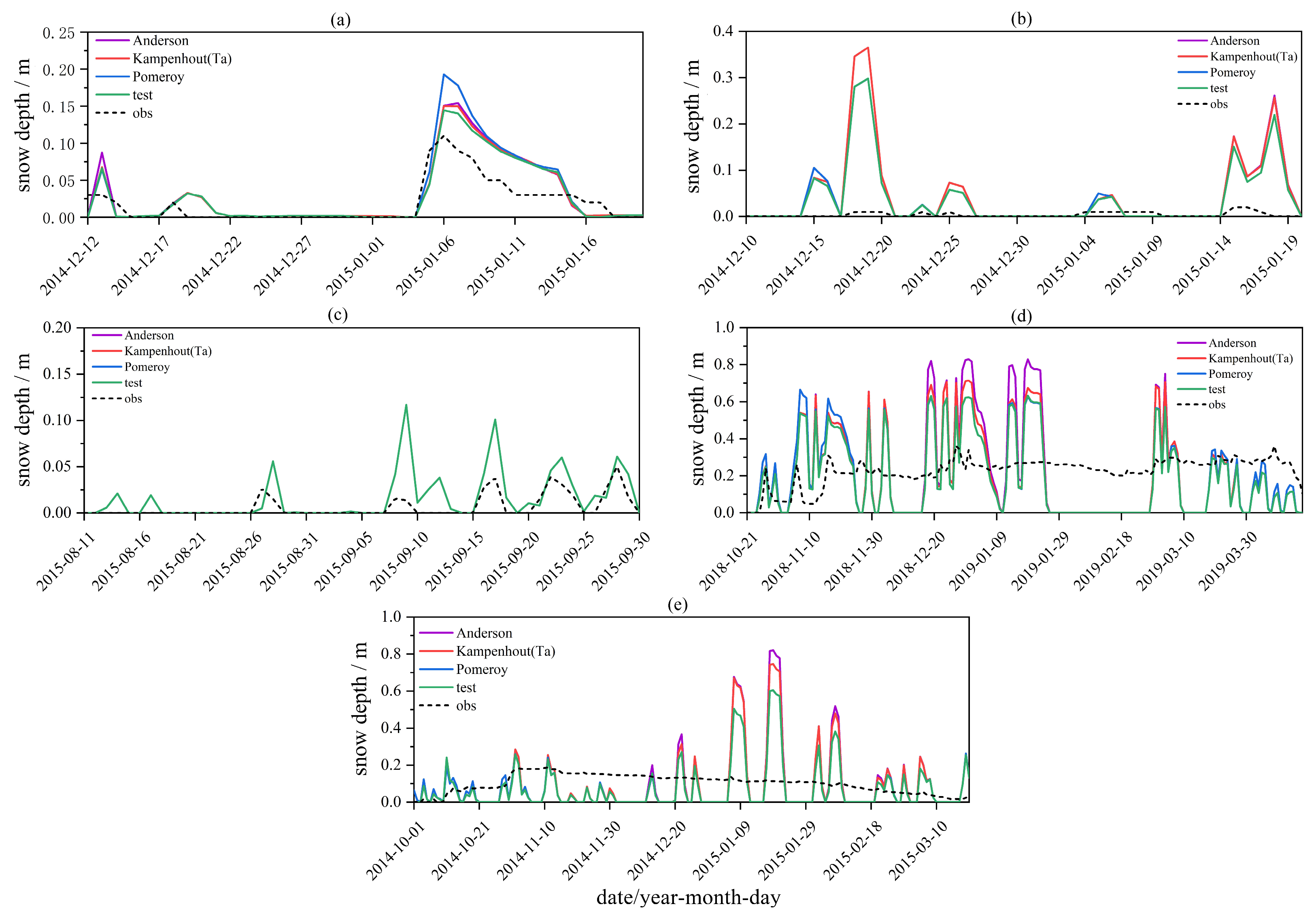
- Although we have found several schemes that improved simulation effects on the discontinuous snow depth, all schemes simulated larger snow depths during the accumulation process and earlier ablation characteristics of continuous snow cover process. The Tibetan Plateau (TP) has a dry and cold climate, resulting in a low snow density under low temperature and humidity conditions. Consequently, the model produces exaggerated snow depths due to the same rainfall forcing data. Additionally, during snow melting, the melted water penetrates the snow layer and freezes into ice, leading to a significant increase in snow density. However, due to climate dryness on the TP, it causes the model to overestimate the rates of snowmelt and snow density caused by the refreezing of meltwater [62].
- (2)
- The snow cover fraction (SCF) is usually less than 100%; yet, for local scale-like site observations, the SCF should be 100% once the snow depth is more than a certain threshold. Otherwise, a less than 100% SCF will remarkably reduce surface albedo and enhance snow melting, leading to smaller SCFs; this positive feedback leads to quick snow ablation in continuous snow cover processes. Furthermore, solar radiation, air temperature, precipitation, and the orientation of the slope are crucial factors in the snowmelt modeling process [63,64,65]. Therefore, other parameterization schemes in the model need to be further evaluated to improve the land surface process model for continuous snow cover on the TP in the future.
- (3)
- Due to the limited availability of snow depth and precipitation observation data in the field at the Maqu and Madoi stations, this study utilized the products of snowfall and precipitation at the station where the China Meteorological Administration was located, or where the precipitation was observed in the field. The analyzed data were strictly controlled, but it was still impossible to completely avoid the deviation of the model from the snow simulation due to the insufficient accuracy of the precipitation-forced input. At present, various remote sensing snow monitoring data can compensate for the shortage of observation stations and snow parameters on the plateau [66,67,68]. We hope to fully utilize these two types of data in the future and carry out more comprehensive and accurate studies on the plateau snow.
- (4)
- Further improvements are required in the calculation method used in this study to compare surface soil heat flux with the model outputs. From the comparison, the calculation results of soil heat flux were very different from the simulation, and the energy non-closure rate during the snow accumulation process was large [69]. A detailed consideration of energy dissipation during transmission processes will enable a better verification and evaluation of land surface process model capabilities.
5. Conclusions
- (1)
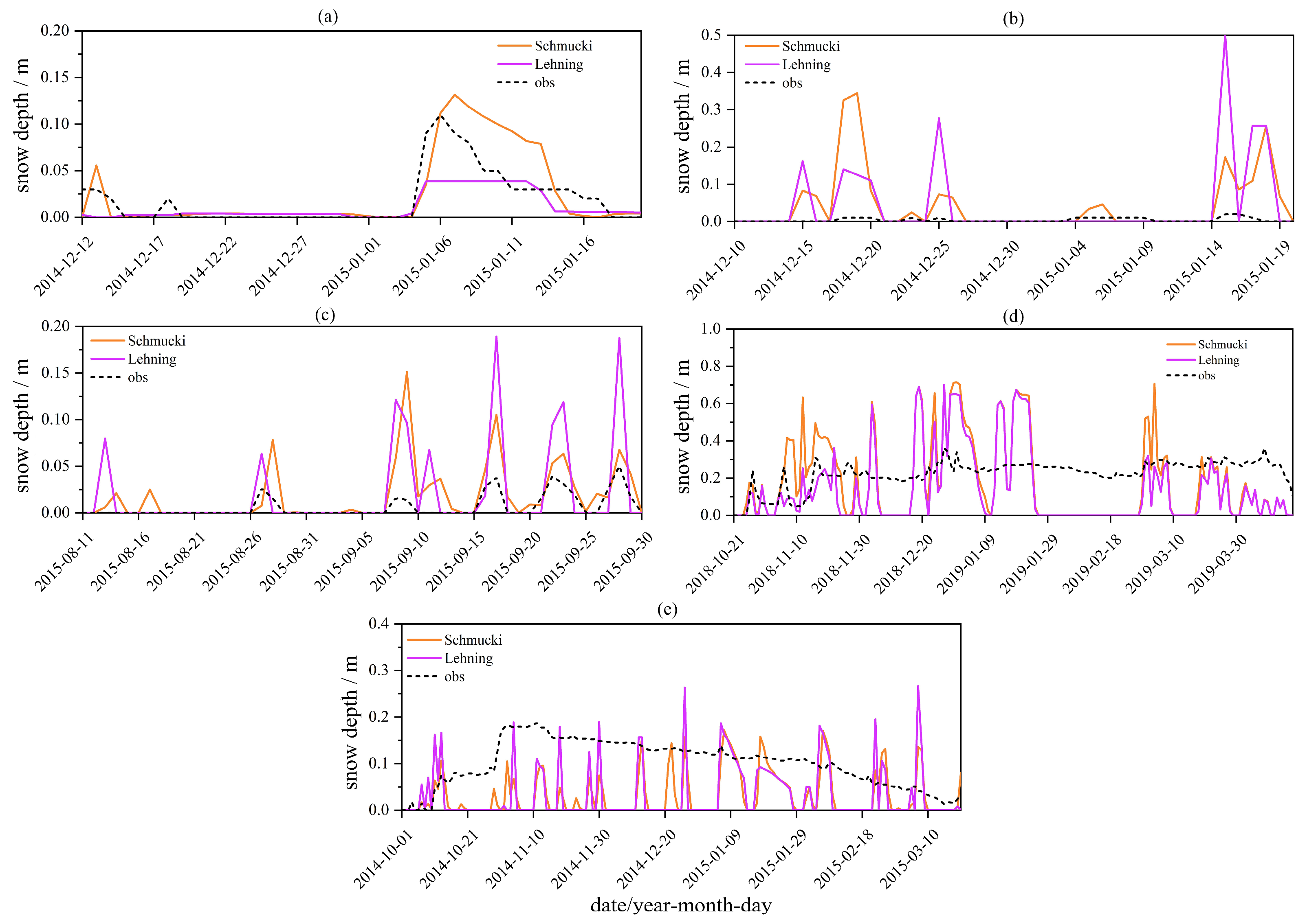
- All schemes can simulate the accumulation and ablation process of discontinuous snow cover in a short period at three stations, and the KW scheme (adding the wind speed calculation component) was the best-performing scheme regarding snow depth simulation. However, no scheme was able to adequately describe the continuous accumulation of snow cover with the characters of repeated accumulation and ablation at Madoi and Yakou for a long period of time. Under the circumstances, the Lehning scheme performed marginally better than other schemes in terms of snow depth during continuous snow.
- (2)
- Compared with other schemes, the simulation effect of the Schmucki scheme on radiation flux and energy flux under discontinuous snow cover was significantly improved.
- (3)
- According to the simulation effects of the improved fresh snow density scheme on the radiation and energy flux in the discontinuous snow process, the change in upward longwave radiation has a negative correlation with the snow depth; that is, the snow accumulation has an overall effect on cooling when the snow depth is less than 20 cm, and the upward shortwave radiation may either decrease or increase with increasing snow depth. The simulated depth of snow has a considerable effect on the heat exchange (sensible heat flux and latent heat flux) between the ground and air, demonstrating that the effective thermal conductivity in the model is sensitive to varying snow density responses.
Supplementary Materials
Author Contributions
Funding
Institutional Review Board Statement
Informed Consent Statement
Data Availability Statement
Acknowledgments
Conflicts of Interest
References
- Henderson, G.R.; Peings, Y.; Furtado, J.C.; Kushner, P.J. Snow–atmosphere coupling in the Northern Hemisphere. Nat. Clim. Chang. 2018, 8, 954–963. [Google Scholar] [CrossRef]
- Qin, D.H.; Zhou, B.T.; Xiao, C.D. Progress in studies of cryospheric changes and their impacts on climate of China. Acta Meteorol. Sin. 2014, 72, 869–879. [Google Scholar] [CrossRef]
- Cohen, J. Snow cover and climate. Weather 1994, 49, 150–156. [Google Scholar] [CrossRef]
- Déry, S.J.; Brown, R.D. Recent Northern Hemisphere snow cover extent trends and implications for the snow-albedo feedback. Geophys. Res. Lett. 2007, 34, 60–64. [Google Scholar] [CrossRef]
- Bo, Y.; Li, X.L.; Wang, C.H. Seasonal characteristics of the interannual variations centre of the Tibetan Plateau snow cover. J. Glaciol. Geocryol. 2014, 36, 1353–1362. [Google Scholar]
- Wang, C.H.; Wang, Z.L.; Cui, Y. Snow Cover of China during the Last 40 Years: Spatial Distribution and Interannual Variation. J. Glaciol. Geocryol. 2009, 31, 301–310. [Google Scholar]
- Pu, Z.X.; Xu, L.; Salomonson, V.V. MODIS/Terra observed seasonal variations of snow cover over the Tibetan Plateau. Geophys. Res. Lett. 2007, 34, 137–161. [Google Scholar] [CrossRef]
- Li, W.; Guo, W.; Qiu, B.; Xue, Y.; Hsu, P.-C.; Wei, J. Influence of Tibetan Plateau snow cover on East Asian atmospheric circulation at medium-range time scales. Nat. Commun. 2018, 9, 4243. [Google Scholar] [CrossRef] [PubMed]
- Zhou, Y.; Jiang, J.; Huang, A.; La, M.; Zhao, Y.; Zhang, L. Possible contribution of heavy pollution to the decadal change of rainfall over eastern China during the summer monsoon season. Environ. Res. Lett. 2013, 8, 044024. [Google Scholar] [CrossRef][Green Version]
- Wang, S.J. Progresses in variability of snow cover over the Qinghai-Tibetan Plateau and its impact on water resources in China. Plateau Meteorol. 2017, 36, 1153–1164. [Google Scholar]
- Duan, A.; Xiao, Z.; Wu, G.; Wang, M. Study Progress of the Influence of the Tibetan Plateau Winter and Spring Snow Depth on Asian Summer Monsoon. Meteorol. Environ. Sci. 2014, 7, 94–101. [Google Scholar] [CrossRef]
- Li, D.L.; Wang, C.X. Research progress of snow cover and its influence on China climate. Trans. Atmos. Sci. 2011, 34, 627–636. [Google Scholar] [CrossRef]
- Zhao, H.X.; Moore, G.W.K. On the relationship between Tibetan snow cover, the Tibetan plateau monsoon and the Indian summer monsoon. Geophys. Res. Lett. 2004, 31, 101–111. [Google Scholar] [CrossRef]
- Li, H.Y.; Wang, J. Key research topics and their advances on modeling snow hydrological process. J. Glaciol. Geocryol. 2013, 35, 430–437. [Google Scholar]
- Duan, A.M.; Xiao, Z.X.; Wang, Z.Q. mpacts of the Tibetan Plateau winter/spring snow depth and surface heat source on Asian summer monsoon: A review. Chin. J. Atmos. Sci. 2018, 42, 755–766. [Google Scholar] [CrossRef]
- Flanner, M.G.; Shell, K.M.; Barlage, M.; Perovich, D.K.; Tschudi, M.A. Radiative forcing and albedo feedback from the northern hemisphere cryosphere between 1979 and 2008. Nat. Geoence 2013, 4, 151–155. [Google Scholar] [CrossRef]
- Groisman, P.Y.; Karl, T.R.; Knight, R.W. Observed impact of snow cover on the heat balance and the rise of continental spring temperatures. Science 1994, 263, 198–200. [Google Scholar] [CrossRef]
- Shugar, D.H.; Jacquemart, M.; Shean, D.; Bhushan, S.; Upadhyay, K.; Sattar, A.; Schwanghart, W.; McBride, S.; De Vries, M.V.W.; Mergili, M.; et al. A massive rock and ice avalanche caused the 2021 disaster at Chamoli, Indian Himalaya. Science 2021, 373, 300–306. [Google Scholar] [CrossRef]
- Peng, S.; Piao, S.; Ciais, P.; Friedlingstein, P.; Zhou, L.; Wang, T. Change in snow phenology and its potential feedback to temperature in the Northern Hemisphere over the last three decades. Environ. Res. Lett. 2013, 8, 1880–1885. [Google Scholar] [CrossRef]
- Barnett, T.P.; Adam, J.C.; Lettenmaier, D.P. Potential impacts of a warming climate on water availability in snow-dominated regions. Nature 2005, 438, 303–309. [Google Scholar] [CrossRef]
- Goulden, M.L. Sensitivity of Boreal Forest Carbon Balance to Soil Thaw. Science 1998, 279, 214–217. [Google Scholar] [CrossRef] [PubMed]
- Ke, C.Q.; Li, P.J. Spatial and temporal characteristic of snow cover over the Qinghai-Xizang Plateau. Acta Geogr. Sin. 1998, 53, 209–215. [Google Scholar]
- Robinson, D.A.; Frei, A.; Serreze, M.C. Recent variations and regional relationships in Northern Hemisphere snow cover. Ann. Glaciol. 1995, 21, 71–76. [Google Scholar] [CrossRef]
- Zhang, H.H.; Jiang, H.M.; Chen, Q.; Xiao, U. Influence of Snow Cover on Soil Temperature, Soil Moisture and Surface Energy Budget at Alpine Meadow. Plateau Meteorol. 2020, 39, 740–749. [Google Scholar] [CrossRef]
- Jiang, Q.; Luo, S.; Wen, X.; Lyu, S. Spatial-temporal Characteristics of Snow and Influence Factors in the Qinghai-Tibetan Plateau from 1961 to 2014. Plateau Meteorol. 2020, 39, 24–36. [Google Scholar] [CrossRef]
- Che, T.; Hao, X.H.; Dai, L.Y.; Li, H.Y.; Huang, X.D.; Xiao, L. Snow Cover Variation and Its Impacts over the Qinghai-Tibet Plateau. Bull. Chin. Acad. Sci. 2019, 34, 1247–1253. [Google Scholar] [CrossRef]
- Xu, W.; Ma, L.; Ma, M.; Zhang, H.; Yuan, W. Spatial–Temporal Variability of Snow Cover and Depth in the Qinghai–Tibetan Plateau. J. Clim. 2017, 30, 1521–1533. [Google Scholar] [CrossRef]
- Wang, T.; Peng, S.S.; Ottlé, C.; Ciais, P. Spring snow cover deficit controlled by intraseasonal variability of the surface energy fluxes. Environ. Res. Lett. 2015, 10, 024018. [Google Scholar] [CrossRef]
- Roebber, P.J.; Bruening, S.L.; Schultz, D.M.; Cortinas, J.V. Improving snowfall forecasting by diagnosing snow density. Weather. Forecast. 2003, 18, 264–287. [Google Scholar] [CrossRef]
- Gong, Y.; Zhou, X.S.; Pan, X.; Bai, H. Advances in newly-fallen snow density research. Torrential Rain Disasters 2020, 39, 325–334. [Google Scholar]
- Loth, B.; Graf, H.-F.; Oberhuber, J.M. Snow cover model for global climate simulations. J. Geophys. Res. 1993, 98, 10451. [Google Scholar] [CrossRef]
- van Kampenhout, L.; Lenaerts, J.T.M.; Lipscomb, W.H.; Sacks, W.J.; Lawrence, D.M.; Slater, A.G.; Broeke, M.R.v.D. Improving the Representation of Polar Snow and Firn in the Community Earth System Model. J. Adv. Model. Earth Syst. 2017, 9, 2583–2600. [Google Scholar] [CrossRef]
- Vionnet, V.; Brun, E.; Morin, S.; Boone, A.; Faroux, S.; Le Moigne, P.; Martin, E.; Willemet, J.-M. The detailed snowpack scheme Crocus and its implementation in SURFEX v7. Geosci. Model Dev. Discuss. 2011, 4, 2365–2415. [Google Scholar] [CrossRef]
- Lehning, M.; Bartelt, P.; Brown, B.; Fierz, C. A physical SNOWPACK model for the Swiss avalanche warning: Part III: Meteorological forcing, thin layer formation and evaluation. Cold Reg. Sci. Technol. 2002, 35, 169–184. [Google Scholar] [CrossRef]
- Pomeroy, J.W.; Gray, D.M.; Shook, K.R.; Toth, B.; Essery, R.L.H.; Pietroniro, A.; Hedstrom, N. An evaluation of snow accumulation and ablation processes for land surface modelling. Hydrol. Process. 1998, 12, 2339–2367. [Google Scholar] [CrossRef]
- Anderson, E.A. A Point Energy Balance Model of a Snow Cover. Office of Hydrology; NOAA Technical Report NWS19; National Weather Service: Fort Worth, TX, USA, 1976.
- Dubé, I. From mm to cm Study of Snow/Liquid Water Ratios in Quebec; MSC-Quebec region; Metropolitan Edison Co.: Akron, ON, USA, 2003; pp. 1–127. [Google Scholar]
- Ma, L.J.; Qin, D.H. Spatial-Temporal Characteristics of Observed Key Parameters for Snow Cover in China during 1957–2009. J. Glaciol. Geocryol. 2012, 34, 1–11. [Google Scholar]
- Bruland, O.; Færevåg, Å.; Steinsland, I.; Liston, G.E.; Sand, K. Weather SDM: Estimating snow density with high precision using snow depth and local climate. Hydrol. Res. 2015, 46, 494–506. [Google Scholar] [CrossRef]
- Yao, C.; Lyu, S.H.; Li, Z.G.; Fang, X.W.; Zhang, S.B. Simulation of the Snow Cover Influence in the Source Region of the Yellow River on the Hydrothermal Process of Frozen Soil. Plateau Meteorol. 2020, 39, 1167–1180. [Google Scholar] [CrossRef]
- Xie, Z.; Hu, Z.; Xie, Z.; Jia, B.; Sun, G.; Du, Y.; Song, H. Impact of the snow cover scheme on snow distribution and energy budget modeling over the Tibetan Plateau. Theor. Appl. Climatol. 2018, 131, 951–965. [Google Scholar] [CrossRef]
- Zhong, W. Investigation on Deformation of Thermokarst Terrain in Permafrost Regions over Heihe River Basin in Qilian Mountains. Master’s Thesis, Lanzhou University, Lanzhou, China, 2019. [Google Scholar]
- Luo, S.; Fang, X.; Lyu, S.; Zhang, Y.; Chen, B. Improving CLM4.5 simulations of land-atmosphere exchange during freeze-thaw processes on the Tibetan Plateau. J. Meteorol. Res. 2017, 31, 916–930. [Google Scholar] [CrossRef]
- Hou, Y.T. High-Resolution Precipitation Driving Analysis and Runoff Response Simulation of NOAH-LSM in the Upper Reaches of the Heihe River Basin; Lanzhou University: Lanzhou, China, 2013. [Google Scholar]
- Hao, X.H.; Wang, J.; Che, T.; Zhang, P.; Liang, J.; Li, H.; Li, Z.; Bai, Y.; Bai, Y. The Spatial Distribution and Properties of Snow Cover in Binggou Watershed, Qilian Mountains: Measurement and Analysis. J. Glaciol. Geocryol. 2009, 31, 284–292. [Google Scholar]
- Liu, S.; Che, T.; Xu, Z.; Zhang, Y.; Tan, J.; Ren, Z.; Li, X. Qilian Mountains Integrated Observatory Network: Dataset of Heihe Integrated Observatory Network (Automatic Weather Station of Yakou Station, 2021); National Tibetan Plateau Data Center: Lanzhou, China, 2022. [CrossRef]
- Che, T.; Liu, S.M.; Li, X.; Xu, Z.W.; Zhang, Y.; Tan, J.L. Observation of Water and Heat Flux in Alpine Meadow Ecosystem—Automatic Weather Station of Yakou Station (2015–2017); National Tibetan Plateau Data Center: Lanzhou, China, 2019. [CrossRef]
- Liu, S.; Li, X.; Xu, Z.; Che, T.; Xiao, Q.; Ma, M.; Liu, Q.; Jin, R.; Guo, J.; Wang, L.; et al. The Heihe Integrated Observatory Network: A Basin-Scale Land Surface Processes Observatory in China. Vadose Zone J. 2018, 17, 1–21. [Google Scholar] [CrossRef]
- Liu, S.M.; Xu, Z.W.; Wang, W.Z.; Jia, Z.Z.; Zhu, M.J.; Bai, J.; Wang, J.M. A comparison of eddy-covariance and large aperture scintillometer measurements with respect to the energy balance closure problem. Hydrol. Earth Syst. Sci. 2011, 15, 1291–1306. [Google Scholar] [CrossRef]
- Li, W.; Luo, S.; Hao, X.; Wang, J.; Wang, Y. Observations of East Qinghai-Xizang Plateau Snow Cover Effects on Surface Energy and Water Exchange in Different Seasons. Plateau Meteorol. 2021, 40, 455–471. [Google Scholar] [CrossRef]
- Li, H.Y.; Wang, J.; Bai, Y.J.; Li, Z.; Dou, Y. The Snow Hydrological Processes during a Representative Snow Cover Period in Binggou Watershed in the Upper Reaches of Heihe River. J. Glaciol. Geocryol. 2009, 2, 293–300. [Google Scholar]
- Hu, H.R.; Liang, L. Spatial and temporal variations of winter snow over east of Qinghai-Tibet Plateau in the last 50 years. Acta Geogr. Sin. 2013, 68, 1493–1503. [Google Scholar] [CrossRef]
- Wei, Z.G.; Huang, R.H.; Chen, W.; Dong, W.J. Spatial Distributions and Interdecadal Variations of the Snow at the Tibetan Plateau Weather Stations. Atmos. Sci. 2002, 26, 496–508. [Google Scholar]
- Zhao, H.L.; Zhou, R.L.; Zhao, Y. Snow Ecology; China Ocean Press: Beijing, China, 2003. [Google Scholar]
- Zhang, H.; Xiao, J.; Chen, Q.; Jiang, H. Micro-meteorological characteristics analysis of two snowfall processes in Gande of Qinghai Province. Meteorol. Mon. 2019, 45, 1093–1103. [Google Scholar]
- Swenson, S.C.; Lawrence, D.M. A New Fractional Snow Covered Area Parameterization for the Community Land Model and its Effect on the Surface Energy Balance. J. Geophys. Res. Atmos. 2012, 117, D21107. [Google Scholar] [CrossRef]
- Oleson, K.W.; Lawrence, D.M.; Bonan, G.B. Technical description of version 4.5 of the Community Land Model (CLM). Ncar Tech. Note NCAR/TN-503 + STR. National Center for Atmospheric Research, Boulder. Geophys. Res. Lett. 2013, 37, 256–265. [Google Scholar] [CrossRef]
- Lawrence, D.M.; Slater, A.G. The contribution of snow condition trends to future ground climate. Clim. Dyn. 2009, 34, 969–981. [Google Scholar] [CrossRef]
- Jordan, R. A One-Dimensional Temperature Model for a Snow Cover: Technical Documentation for SNTHERM; DTIC: Lincoln, NE, USA, 1991.
- Anderson, E.A. A Point Energy and Mass Balance Model of a Snow Cover. NOAA Tech. Rep. 1976 NWS 19, 150p. Available online: http://amazon.nws.noaa.gov/articles/HRL_Pubs_PDF_May12_2009/HRL_PUBS_51-100/81_A_POINT_ENERGY_AND_MASS.pdf (accessed on 10 September 2022).
- Dai, Y.; Zeng, Q. A land surface model (IAP94) for climate studies. Part I: Formulation and validation in off-line experiments. Adv. Atmos. Sci. 1997, 14, 433–460. [Google Scholar]
- Toure, A.M.; Luojus, K.; Rodell, M.; Getirana, A. Evaluation of simulated snow and snowmelt timing in the Community Land Model using satellite-based products and streamflow observations. J. Adv. Model. Earth Syst. 2018, 10, 2933–2951. [Google Scholar] [CrossRef] [PubMed]
- Mioduszewski, J.R.; Rennermalm, A.K.; Robinson, D.A.; Mote, T.L. Attribution of snowmelt onset in northern Canada. J. Geophys. Res. Atmos. 2014, 119, 9638–9653. [Google Scholar] [CrossRef]
- Zhao, H.L.; Li, H.Y.; Xuan, Y.Q.; Bao, S.; Cidan, Y.; Liu, Y.; Li, C.; Yao, M. Investigating the critical influencing factors of snowmelt runoff and development of a mid-long term snowmelt runoff forecasting. J. Geogr. Sci. 2023, 33, 1313–1333. [Google Scholar] [CrossRef]
- Zhang, F.; Zhang, H.B.; Hagen, S.C.; Ye, M.; Wang, D.; Gui, D.; Zeng, C.; Tian, L.; Liu, J. Snow cover and runoff modelling in a high mountain catchment with scarce data: Effects of temperature and precipitation parameters. Hydrol. Process. 2015, 29, 52–65. [Google Scholar] [CrossRef]
- Park, S.E. Variations of Microwave Scattering Properties by Seasonal Freeze/Thaw Transition in the Permafrost Active Layer Observed by ALOS PALSAR Polarimetric Data. Remote Sens. 2015, 7, 17135–17148. [Google Scholar] [CrossRef]
- Usami, N.; Muhuri, A.; Bhattacharya, A.; Hirose, A. Proposal of Wet Snow Mapping with Focus on Incident Angle Influential to Depolarization of Surface Scattering. In Proceedings of the 2016 IEEE International Geoscience and Remote Sensing Symposium (IGARSS), Beijing, China, 10–15 July 2016; IEEE: Piscataway, NJ, USA, 2016. [Google Scholar] [CrossRef]
- Tsai, Y.-L.S.; Dietz, A.; Oppelt, N.; Kuenzer, C. Remote Sensing of Snow Cover Using Spaceborne SAR: A Review. Remote Sens. 2019, 11, 1456. [Google Scholar] [CrossRef]
- Ge, J.; Yu, Y.; Li, Z.; Jie, J.; Liu, C.; Zai, B. Impacts of Freeze/Thaw Processes on Land Surface Energy Fluxes in the Permafrost Region of Qinghai-Xizang Plateau. Plateau Meteorol. 2016, 35, 608–620. [Google Scholar]


| Scheme | Statistic | ULR | USR | Rn | Hs | LE | G0 |
|---|---|---|---|---|---|---|---|
| Schmucki | ME | 16.65 | −24.72 | 8.07 | 4.68 | 8.09 | −10.39 |
| RMSE | 22.31 | 66.28 | 59.74 | 37.58 | 21.19 | 90.67 | |
| Kw | ME | 14.30 | −24.51 | 10.21 | −0.10 | 16.00 | −11.32 |
| RMSE | 20.53 | 68.75 | 63.45 | 37.57 | 28.27 | 87.51 | |
| Anderson | ME | 13.91 | −24.54 | 10.63 | −0.36 | 15.49 | −10.06 |
| RMSE | 20.08 | 68.52 | 63.33 | 37.07 | 27.66 | 87.38 |
| Scheme | Statistic | ULR | USR | Rn | Hs | LE | G0 |
|---|---|---|---|---|---|---|---|
| Schmucki | ME | 19.84 | −71.29 | 51.45 | 44.17 | 53.06 | 16.62 |
| RMSE | 25.66 | 138.73 | 117.55 | 65.60 | 81.73 | 90.41 | |
| Kw | ME | 20.10 | −72.30 | 52.20 | 44.92 | 53.57 | 16.33 |
| RMSE | 25.84 | 139.62 | 118.30 | 66.02 | 81.97 | 90.64 | |
| Anderson | ME | 20.10 | −72.30 | 52.20 | 44.92 | 53.57 | 16.33 |
| RMSE | 25.84 | 139.62 | 118.30 | 66.02 | 81.97 | 90.64 |
Disclaimer/Publisher’s Note: The statements, opinions and data contained in all publications are solely those of the individual author(s) and contributor(s) and not of MDPI and/or the editor(s). MDPI and/or the editor(s) disclaim responsibility for any injury to people or property resulting from any ideas, methods, instructions or products referred to in the content. |
© 2023 by the authors. Licensee MDPI, Basel, Switzerland. This article is an open access article distributed under the terms and conditions of the Creative Commons Attribution (CC BY) license (https://creativecommons.org/licenses/by/4.0/).
Share and Cite
Li, W.; Luo, S.; Wang, J.; Wang, Y. Evaluation of Ten Fresh Snow Density Parameterization Schemes for Simulating Snow Depth and Surface Energy Fluxes on the Eastern Tibetan Plateau. Atmosphere 2023, 14, 1571. https://doi.org/10.3390/atmos14101571
Li W, Luo S, Wang J, Wang Y. Evaluation of Ten Fresh Snow Density Parameterization Schemes for Simulating Snow Depth and Surface Energy Fluxes on the Eastern Tibetan Plateau. Atmosphere. 2023; 14(10):1571. https://doi.org/10.3390/atmos14101571
Chicago/Turabian StyleLi, Wenjing, Siqiong Luo, Jingyuan Wang, and Yuxuan Wang. 2023. "Evaluation of Ten Fresh Snow Density Parameterization Schemes for Simulating Snow Depth and Surface Energy Fluxes on the Eastern Tibetan Plateau" Atmosphere 14, no. 10: 1571. https://doi.org/10.3390/atmos14101571
APA StyleLi, W., Luo, S., Wang, J., & Wang, Y. (2023). Evaluation of Ten Fresh Snow Density Parameterization Schemes for Simulating Snow Depth and Surface Energy Fluxes on the Eastern Tibetan Plateau. Atmosphere, 14(10), 1571. https://doi.org/10.3390/atmos14101571