Improvement and Comparison of Multi-Reference Station Regional Tropospheric Delay Modeling Method Considering the Effect of Height Difference

Abstract

Tropospheric delay information is particularly important for network RTK (Network Real-time Kinematic) positioning. Conventionally, tropospheric delay information at a virtual reference station (VRS) is obtained using the linear interpolation method (LIM). However, the conventional LIM cannot work well when there is a substantial height difference between the rover station and the reference station. Consequently, we propose a modified linear interpolation method (MLIM) by carefully handling the height difference between the rover station and the reference station. The new MLIM method first corrects the systematic error of the double-difference (DD) tropospheric delay in the elevation direction caused by the height difference, and then utilizes the linear interpolation algorithm to obtain the tropospheric delay of the VRS station. To determine the parameters of the low-order surface model (LSM), we also propose a modified LSM (MLSM) interpolation method in the triangular network and evaluate it in the positioning domains. The two new interpolation methods are evaluated using two regional GNSS networks with obvious height disparities. Results show that the DD tropospheric delay interpolation accuracy obtained by the new MLIM and MLSM is improved by 56.5% and 78.7% on average in the two experiments compared to the conventional method. The new MLIM and MLSM are more accurate than the traditional LIM (TLIM) in cases with low elevation satellites. Additionally, the positioning accuracies are improved by using the MLIM and MLSM methods. The MLIM and MLSM outperform TLIM in the up-component by an average of 72.8% and 80.7%, respectively.

1. Introduction

Due to the influence of the atmosphere, orbit, and other distance-related errors, traditional single-station RTK positioning technology restricts the distance between the mobile station and the reference station to approximately 10 km in order to achieve centimeter-level positioning accuracy. Real-time high-precision positioning services can now cover a range of tens or even hundreds of kilometers thanks to the development of network RTK technology, which is based on evenly distributed GNSS reference stations within the regional range [1]. Virtual reference station (VRS) technology is widely promoted and used in many network RTK solutions [2]. Double-difference (DD) ionosphere, troposphere, and other delays can be precisely resolved when the ambiguity of the network baseline generated between the reference stations is accurately determined. These errors are then interpolated to obtain errors such as atmospheric delays on VRS stations near the rover station. Lastly, using these interpolated delays, the VRS station’s virtual observations can be created. The user can then employ such observations to resolve the short baseline rapidly and achieve real-time high-precision coordinate information [3,4,5].

The key issue in network RTK is choosing an effective and appropriate method to create virtual observations after successfully resolving the atmospheric delay on the network baseline [4]. As a result, a variety of interpolation models and methods have been proposed by researchers for atmospheric delays. Wanninger first proposed the linear interpolation method (LIM), which requires at least three reference stations around the VRS station. The LIM uses dual-frequency phase observations and the known coordinate information of the reference station, thereby establishing a regional atmospheric delay model in the coverage area of the reference station through the difference in the plane coordinates between the reference station and the VRS station [5]. Han and Rizos proposed a linear combinatorial model (LCM), which is mainly used to eliminate orbital errors but can also be used to model atmospheric delays [6]. Gao et al. considered that a different distance between each reference station and VRS station and proposed a distance-dependent interpolation method (DIM). However, this method is mainly used for interpolated ionospheric errors [7]. Wübbena proposed to use an appropriate trend surface or low-order surface model (LSM) to simulate the trend of distance-related errors in the network, thus achieving the purpose of atmospheric modeling [8]. The benefits and drawbacks of the main atmospheric interpolation algorithms and models listed above (Dai et al., Fotopoulos et al., Wu et al., and Al-Shaery et al.) have been investigated and examined, with research finding similar impacts between them [9,10,11,12]. It is challenging to determine which algorithm is best. However, in a triangular network divided by traditional triangulation, the rover station is usually surrounded by a triangular cell, so the linear interpolation method using three reference stations is widely used due to its simple implementation and strong applicability.

The correlation of tropospheric delays decreases as the length of the network baseline increases, resulting in an increase in residual errors in the double-difference observations. Excessive errors will affect the fuzzy solution and positioning accuracy [13]. Due to the strong correlation between tropospheric delay and height, the correlation coefficient between them exceeds 0.9 [14]. Thus, the tropospheric error caused by an obvious height difference will seriously affect the solution of the station coordinates [15]. Landau experimented with data from the German SAPOS network and found that when there is a significant height difference between the reference station and the rover, the tropospheric systematic error can reach 6.8 cm [16]. Since the above interpolation methods only considers the distribution of the troposphere in the horizontal direction, if these methods are used directly within a triangular unit, the troposphere delay on the interpolated VRS station will be strongly constrained to the plane formed by the reference station, and the tropospheric delay distributed in the vertical direction will be completely ignored. With this in mind, Wu et al. proposed a multi-baseline tropospheric delayed interpolation method that is more accurate than linear interpolation in star networks [17]. In addition, using the BP neural network method, Qiu et al. obtained better tropospheric delay accuracy by training sample data and established a spatial tropospheric error model [18]. Shi et al. suggested an optimal fitting model for obtaining the troposphere’s local fitting coefficients. The user is then provided determined troposphere fitting coefficients in order to shorten the PPP convergence time [19]. Based on the PPP model, Zhang and Zheng proposed a large-scale improved tropospheric model for China [20,21,22]. These two models can effectively correct tropospheric delays and enhance PPP precision.

The main purpose of this paper is to use the two proposed interpolation algorithm to improve the accuracy of tropospheric delay corrections in network RTK and to obtain more stable and reliable positioning results, especially in the elevation direction. It should be noted that in NRTK, when there is a significant height difference between the Continuously Operating Reference Station (CORS) reference station and rover, the conventional tropospheric interpolation method will be affected by the systematic errors caused by the height difference. Ultimately, when there is a significant height difference between the rover and the surrounding reference station, the adoption of TLIM will decrease the tropospheric interpolation accuracy and cause systematic errors. Considering the height difference between the reference station and the rover station, in MLIM, an external priori model of tropospheric delay is first used to correct the tropospheric delay on the solved network baseline, and then the corrected tropospheric delay is interpolated by linear interpolation. In the MLSM, the external constraint of troposphere is introduced as an additional equation, and then the elevation coefficient of the model can be estimated. Finally, the interpolation value is directly used for the generation of virtual observations and the positioning of the rover station.

2. Materials and Methods

Here, we first introduce the acquisition process of the tropospheric delay required to generate the observations on the virtual reference station and then introduce several commonly used tropospheric interpolation methods and models. Lastly, we introduce the modified linear interpolation method and low-order surface model proposed in this paper.

2.1. The Process of Calculating and Modeling Tropospheric Delays on VRS

In order to accurately obtain the double-difference tropospheric delay on the network baseline, an accurate solution for network baseline ambiguity is a prerequisite. The ambiguity solution strategy we adopted is to first solve the wide-lane (WL) ambiguity with a longer wavelength and then use the combined ionosphere-free observations to solve the basic ambiguity [23]. The specific steps are as follows.

First, we use the following observation equation to solve the WL ambiguity:

$$\{\begin{array}{l}{L}_{rb,WL}^{ij}={\rho }_{rb}^{ij}+T_{rb}^{ij}+\frac{f_1}{f_2}(I_{rb,1}^j-I_{rb,1}^i)+{\lambda }_{WL}(N_{rb,WL}^j-N_{rb,WL}^i)+{\epsilon }_{rb,WL}^{ij}\\ L_{rb,1}^{ij}={\rho }_{rb}^{ij}+T_{rb}^{ij}-(I_{rb,1}^j-I_{rb,1}^i)+{\lambda }_1(N_{rb,1}^j-N_{rb,1}^i)+{\epsilon }_{rb,1}^{ij}\\ P_{rb,1}^{ij}={\rho }_{rb}^{ij}+T_{rb}^{ij}+(I_{rb,1}^j-I_{rb,1}^i)+e_{rb,1}^{ij}\\ P_{rb,2}^{ij}={\rho }_{rb}^{ij}+T_{rb}^{ij}+\frac{f_1^2}{f_2^2}(I_{rb,1}^j-I_{rb,1}^i)+e_{rb,2}^{ij}\\ \widetilde{I_{rb,1}^{ij}}=I_{rb,1}^j-I_{rb,1}^i\end{array}$$

(1)

where r and b are the base station and rover station at both ends of the network baseline, and i and j represent the reference satellite and the rover satellite, respectively; $L_{rb,WL}^{ij}$,$L_{rb,1}^{ij}$,$P_{rb,1}^{ij}$, and $P_{rb,2}^{ij}$ are the WL, L1, P1, and P2 DD observations in meters, respectively; and ${\rho }_{rb}^{ij}$ is the DD geometric distance from the satellite pair to the receivers, $T_{rb}^{ij}$ is the DD tropospheric delay for each satellite pair, and $I_{rb,1}^i$ and $I_{rb,1}^j$ are the single-differenced ionospheric delays of the reference and the rover satellite at the L1 frequency.

$N_{rb,WL}^i$, $N_{rb,WL}^j$, $N_{rb,1}^i$, and $N_{rb,1}^j$ are the WL and L1 ambiguities of the reference satellite and rover satellite, respectively. $f_1$ and $f_2$ are the signal frequencies of L1 and L2, respectively. ${\lambda }_{WL}$ and ${\lambda }_1$ are the wavelengths of WL and L1, respectively. ${\epsilon }_{rb,WL}^{ij}$, ${\epsilon }_{rb,1}^{ij}$, $e_{rb,1}^{ij}$, and $e_{rb,2}^{ij}$ represent observation noise and other errors on phase and pseudorange. $\widetilde{I_{rb,1}^{ij}}$ is the ionospheric pseudo-observations.

Then, using the solved WL ambiguity in Equation (1), the L1 ambiguity can be solved with the following observation equation:

$$\{\begin{array}{l}{L}_{rb,IF}^{ij}={\rho }_{rb}^{ij}+T_{rb}^{ij}+\frac{C}{f_1+f_2}(N_{rb,1}^j-N_{rb,1}^i)+\frac{C{f}_2}{f_1^2+f_2^2}{N}_{rb,WL}^{ij}+{\epsilon }_{rb,IF}^{ij}\\ P_{rb,IF}^{ij}={\rho }_{rb}^{ij}+T_{rb}^{ij}+e_{rb,IF}^{ij}\end{array}$$

(2)

where IF stands for the ionospheric combination, which is the calculated WL ambiguity, and other symbols have the same meaning as in Equation (1).

Since the distance between reference stations is usually at least tens of kilometers greater than 100 km, determining ambiguity is challenging. As a result, considering the long-wavelength characteristics of the WL ambiguity and the benefits of being simple to solve, we resolve the single-difference WL ambiguity with Equation (1) and then solve the L1 ambiguity with Equation (2). Additionally, ionospheric delay is a substantial impediment to ambiguity resolution. Here, we introduce ionospheric pseudo-observations and employ an appropriate weighting strategy to deal with the ionosphere. This strategy takes into consideration the spatial and temporal ionospheric delay [24,25]. Usually, the Klobuchar model (or BDGIM) or the IGS Global Ionospheric Grid Model (GIM) can provide pseudo-observations for the ionosphere [26,27]. Since the GIM model has better accuracy, we use GIM here to obtain ionospheric pseudo-observations [28]. Furthermore, the tropospheric hydrostatic delay corrections are calculated through the UNB3m model with the Niell mapping function [29,30], and the residual wet delay part is referred to as the relative tropospheric wet delay (RZTD), which is estimated using a random walk filter [31].

The SD WL, L1 ambiguity, SD ionospheric delay, and RZTD in the above observation equations are estimated using the Kalman filter. Then, the SD ambiguity is converted into DD ambiguity through the transformation matrix, and the DD WL and L1 integer ambiguity values are obtained via the LAMBDA method [32]. The L2 DD ambiguity is then calculated using the linear relationship between the WL and L1 DD ambiguities.

After obtaining the L1 and L2 ambiguities that are precisely fixed as integers, we can calculate the DD tropospheric delay of each satellite pair on each network baseline as follows:

$${\widehat{T}}_{rb}^{ij}=\frac{f_1^2}{f_1^2-f_2^2}(L_{rb,2}^{ij}-{\lambda }_1{\tilde{N}}_{rb,1}^{ij})-\frac{f_2^2}{f_1^2-f_2^2}(L_{rb,2}^{ij}-{\lambda }_2{\tilde{N}}_{rb,2}^{ij})-{\rho }_{rb}^{ij}$$

(3)

where ${\widehat{T}}_{rb}^{ij}$ represents the calculated DD tropospheric delay, and ${\tilde{N}}_{rb,1}^{ij}$ and ${\tilde{N}}_{rb,2}^{ij}$ denote fixed DD ambiguities on L1 and L2 in units of cycles. Due to the high accuracy of phase observations, the impacts of errors such as observation noise and multipath effects are neglected here.

2.2. Traditional Interpolation Techniques and Modified Linear Interpolation Algorithms for Tropospheric Delay

In the area covered by the reference station, the rover is generally located within a triangular unit formed by at least three reference stations, with the reference station closest to the rover referred to as the master reference station and the other two reference stations referred to as auxiliary reference stations. Using the geometric distribution relationships between these reference stations and the rover, researchers developed regional tropospheric models and proposed various representative models. Here, we primarily describe the linear interpolation model (LIM), the modified linear interpolation model (MLIM), and the lower-order surface model (LSM).

2.2.1. LIM

In network RTK, the minimal network unit where the user is generally located has at least three reference stations, and the linear interpolation model of the tropospheric delay of the rover station can be expressed as

$$\widehat{T}=B{X}_{ab}$$

$$\widehat{T}=\left[\begin{array}{c}{\widehat{T}}_{M,1}\\ {\widehat{T}}_{M,2}\\ ⋮\\ {\widehat{T}}_{M,n-1}\end{array}\right]B=\left[\begin{array}{cc}\Delta X_{M,1}& \Delta Y_{M,1}\\ \Delta X_{M,2}& \Delta Y_{M,2}\\ ⋮& ⋮\\ \Delta X_{M,n-1}& \Delta Y_{M,n-1}\end{array}\right]{ X}_{ab}=\left[\begin{array}{c}a\\ b\end{array}\right]$$

(4)

where M represents the master reference station; 1, 2, …, n − 1 represents the auxiliary reference station; $\Delta X$ and $\Delta Y$ indicate the differences in horizontal coordinates between the master and auxiliary reference stations; $\widehat{T}$ represents the calculated tropospheric delay; B represents the coefficient matrix; and X_ab represents the interpolation model coefficient matrix, which can be solved using least squares:

$$X_{ab}={\left(B^{T}B\right)}^{-1}{B}^T\widehat{T}$$

(5)

Then, one can derive the tropospheric delay between the master station and the rover reference station as follows:

$$T_{M,u}^{\mathrm{ij}}=\left[\begin{array}{cc}\Delta X_{M,u}& \Delta Y_{M,u}\end{array}\right]\cdot X_{\mathrm{ab}}=\left[\begin{array}{cc}\Delta X_{M,u}& \Delta Y_{M,u}\end{array}\right]\cdot {\left(B^{T}B\right)}^{-1}{B}^T\widehat{T}$$

(6)

where $T_{M,u}^{\mathrm{ij}}$ is the interpolated DD tropospheric delay between the master reference station and the user station, and $\Delta X_{M,u}$ and $\Delta Y_{M,u}$ are the horizontal coordinate differences between the master reference station and the user station, respectively.

2.2.2. Modified LIM

Considering the spatiotemporal properties of the troposphere’s distribution, the tropospheric delay is influenced by both horizontal and vertical directions. It is evident that the above LIM interpolation model employs only horizontal coordinates to model tropospheric errors and neglects vertical components. This method restricts tropospheric modeling to a specific elevation plane established by the reference stations. When there is a significant height difference between the rover and the selected reference station, there will be a certain error in the tropospheric delay modeled using the traditional LIM interpolation approach, which will result in a drop in the user’s positioning accuracy. Consequently, we propose to first correct the systematic error of tropospheric delay produced by the height difference between the reference station and the rover and then apply linear interpolation to model the tropospheric delay.

Assuming that in a triangle network unit, M is the master reference station, and A and B are the two auxiliary reference stations. V is the VRS station, whose coordinates are the result of standard point positioning (SPP) of the rover.

Before utilizing LIM interpolation, the tropospheric delay on the baseline of the master reference station and the auxiliary reference station must be corrected if the height of the VRS station is significantly higher or lower than the elevation of the reference station. Taking the baseline MA as an example, the calculated tropospheric delay can be described as

$$T_{MA}^{ij}(\Delta h_{MA})=T_A^{ij}(h_A)-T_M^{ij}(h_M)$$

(7)

where $T_{MA}^{ij}(\Delta h_{MA})$ is the calculated DD tropospheric delay of the satellite pair ij on the baseline MA under the height difference $\Delta h_{MA}$. $T_A^{ij}(h_A)$ and $T_M^{ij}(h_M)$ represent the SD tropospheric delays of stations A and M located at heights h_A and h_M, respectively. The correction equation for the SD tropospheric delay for stations A and M is:

$${\overline{T}}_A^{ij}(h_A)=T_A^{ij}(h_A)+T_{CorA}$$

(8)

$${\overline{T}}_M^{ij}(h_M)=T_M^{ij}(h_M)+T_{CorM}$$

(9)

where ${\overline{T}}_A^{ij}(h_A)$ and ${\overline{T}}_M^{ij}(h_M)$ are the corrected SD tropospheric delays at stations A and M.

The following equations are the specific derivations of the correction terms $T_{CorA}$ and $T_{CorM}$:

$$\begin{array}{ll}{T}_{CorA}& =T_A^{ij}(h_V)-T_A^{ij}(h_A)\\ & =ZT{D}_A(h_V)\times (M{F}_A^j(h_V)-M{F}_A^i(h_V))-ZT{D}_A(h_A)\times (M{F}_A^j(h_A)-M{F}_A^i(h_A))\end{array}$$

(10)

$$\begin{array}{ll}{T}_{CorM}& =T_M^{ij}(h_V)-T_M^{ij}(h_M)\\ & =ZT{D}_M(h_V)\times (M{F}_M^j(h_V)-M{F}_M^i(h_V))-ZT{D}_M(h_M)\times (M{F}_M^j(h_M)-M{F}_M^i(h_M))\end{array}$$

(11)

where $h_A$ and $h_V$ are the heights of station A and VRS. $ZT{D}_A(h_A)$ and $ZT{D}_A(h_V)$ are the tropospheric zenith delay (ZTD) at station A with heights $h_A$ and $h_V$, which can be determined using the prior model. $M{F}_A^j(h_A)$, $M{F}_A^i(h_A)$, $M{F}_A^j(h_V)$, and $M{F}_A^j(h_V)$ represent the mapping functions corresponding to satellites i and j at station A with heights of $h_A$ and $h_V$, respectively.

Although the ZTD calculated by the prior model contains certain model errors, the ZTD difference obtained by the prior model at the same horizontal position but at different heights can effectively represent the systematic errors of the tropospheric delay caused by the height difference [33]. Therefore, $T_{CorA}$ and $T_{CorM}$ derived by the prior model continue to possess a high level of corrective accuracy.

We substituted Equations (10) and (11) into Equations (8) and (9), respectively, and replaced $T_A^{ij}(h_A)$ and $T_M^{ij}(h_M)$ in Equation (7) with ${\overline{T}}_A^{ij}(h_A)$ and ${\overline{T}}_M^{ij}(h_M)$ (10). Equation (7) thus becomes

$${\overline{T}}_{MA}^{ij}(\Delta h_{VV})={\overline{T}}_A^{ij}(h_A)-{\overline{T}}_M^{ij}(h_M)=T_A^{ij}(h_V)-T_M^{ij}(h_V)$$

(12)

where ${\overline{T}}_{MA}^{ij}(\Delta h_{VV})$ is the corrected tropospheric delay on the baseline MA. In this paper, the UNB3m is employed in conjunction with the NMF mapping function to compute the correction term of tropospheric system errors. When the systematic errors of the tropospheric delay calculated by the network baseline are corrected, the LIM model is used for interpolation, and the interpolated tropospheric delay between the VRS station and the master reference station is not affected by the tropospheric system due to height difference effect errors.

2.2.3. Modified LSM

The low-order surface fitting model simulates the spatial features of distance-related errors and simplifies the actual error surface to model the dominant spatial-related error trends.

The interpolation coefficient of LSM is usually obtained by least-squares adjustment. Since the order and variables of the selected fitting function are optional, a commonly used fitting function is listed here:

$$V=\mathrm{a}\cdot \Delta X+\mathrm{b}\cdot \Delta Y+c$$

(13)

When there are more than three reference stations distributed near the user station, the above formula can be written as

$$V=A\cdot C$$

(14)

where V represents the error vector associated with the spatial distance between the master reference station m and each auxiliary reference station, such as the tropospheric delay error. A is the coefficient matrix, which is composed of the reference station coordinate differences, and C is the estimated model coefficient.

$$V=\left[\begin{array}{c}{\widehat{V}}_{M,1}\\ {\widehat{V}}_{M,2}\\ ⋮\\ {\widehat{V}}_{M,n-1}\end{array}\right],A=\left[\begin{array}{ccc}\Delta X_{M,1}& \Delta Y_{M,1}& 1\\ \Delta X_{M,2}& \Delta Y_{M,2}& 1\\ ⋮& ⋮& ⋮\\ \Delta X_{M,n-1}& \Delta Y_{M,n-1}& 1\end{array}\right],C=\left[\begin{array}{c}a\\ \begin{array}{l}b\\ c\end{array}\end{array}\right]$$

(15)

The model coefficients can be obtained by least-squares adjustment as:

$$\widehat{C}=\left[\begin{array}{l}\widehat{a}\\ \widehat{b}\\ \widehat{c}\end{array}\right]={(A^{T}A)}^{-1}{A}^{T}V$$

(16)

The atmospheric interpolation result at the user station is then

$$V_{u,n}=\left[\begin{array}{ccc}\Delta X_{u,n}& \Delta Y_{u,n}& 1\end{array}\right]\cdot {\left[\begin{array}{ccc}\widehat{a}& \widehat{b}& \widehat{c}\end{array}\right]}^T=\left[\begin{array}{ccc}\Delta X_{u,n}& \Delta Y_{u,n}& 1\end{array}\right]\cdot {(A^{T}A)}^{-1}{A}^{T}V$$

(17)

However, in a triangle unit, often only two independent atmospheric delays can be acquired, and only two equations can be established. However, these two equations cannot solve the three model coefficients of LSM. Therefore, we propose using an external tropospheric delay model to generate an additional observation as a constraint, which can compensate for the lack of observations in a triangular unit. Assuming that A is the master reference station, B and C are the auxiliary reference stations, and v is the VRS station, the constrained LSM equation is as follows:

$$\{\begin{array}{l}{V}_{A,B}=\mathrm{a}\cdot \Delta X_{A,B}+\mathrm{b}\cdot \Delta Y_{A,B}+c\\ V_{A,C}=\mathrm{a}\cdot \Delta X_{A,C}+\mathrm{b}\cdot \Delta Y_{A,C}+c\\ {\tilde{V}}_{A,v}=\mathrm{a}\cdot \Delta X_{A,v}+\mathrm{b}\cdot \Delta Y_{A,v}+c\end{array}$$

(18)

where ${\tilde{V}}_{A,v}$ is the tropospheric delay between the master station and the VRS station, which is calculated by the UNB3m model in this paper. The other parameters are the same as described above.

3. Results

3.1. Experimental Data

The experimental data were selected from the US CORS network and the Hong Kong Geodetic CORS network. For the experimental analysis, we chose two triangular unit datasets. Figure 1 and Figure 2 depict the plane distribution of stations and the baseline length of the two datasets. The reference station nearest to each rover was chosen as the master reference station; the stations are linked in the figure by a green dashed line. Dataset 1 stations are located in the mid-latitude region, while the stations of dataset 2 are located in the low-latitude region. The observation data gathered on day of year (DOY) 067 in 2022 were chosen for analysis. The cut-off angle was set to 15 degrees, and the sampling interval was 30 s. However, the two datasets correspond to different regions that are affected by the ionosphere in different ways. The Kp index, introduced by Bartels, is updated every three hours and provides a measure of geomagnetic activity [34]. We checked the KP index of DOY 067 in 2022, where the maximum was 2 and the minimum was 0, which indicates that the ionosphere was quiet on that day. The general assuming ionosphere single-layer model (SLM) has a height of approximately 350 km; therefore, when different satellite signals pass through the ionosphere, these ionospheric pierce points (IPP) are approximately distributed on a plane, and linear interpolation is suited for ionospheric delay modeling. Therefore, the DD ionospheric delay was sufficiently accurate and did not influence the modeling of the tropospheric delay.

The station height distribution of the two datasets is shown in Figure 3. The blue bar indicates the height of the reference stations, whereas the red bar denotes the height of the rovers. In the US CORS dataset 1, the height difference between the rover and the reference stations is considerable, reaching a maximum of 672 m. The height difference between the rover and the reference stations in the Hong Kong CORS dataset 2 is relatively small but still has a maximum of 224 m. This result shows that there is a significant height difference between the reference station and the rover in the two datasets.

We utilized the latest up-to-date Canadian Spatial Reference System Precise Point Positioning (CSRS-PPP) solution service provided by Natural Resources Canada to obtain the ZTDs of both the rover and the primary reference station. Since the estimation precision of this service can approach 0.2 cm, the tropospheric slant DD delay determined by the projection function can be regarded as the true value [35,36,37,38,39]. During data processing, the STDs of the phase and pseudorange observations were set to 0.003 and 0.3 m, respectively. Antenna phase center corrections, and other errors were ignored. In a complicated mountain environment, different components, such as mountain reflection, could lead to the multipath effect. Real measurement should be conducted in an environment with an open sky. This, however, is not the primary error in our research, thus it will not be discussed in detail here.

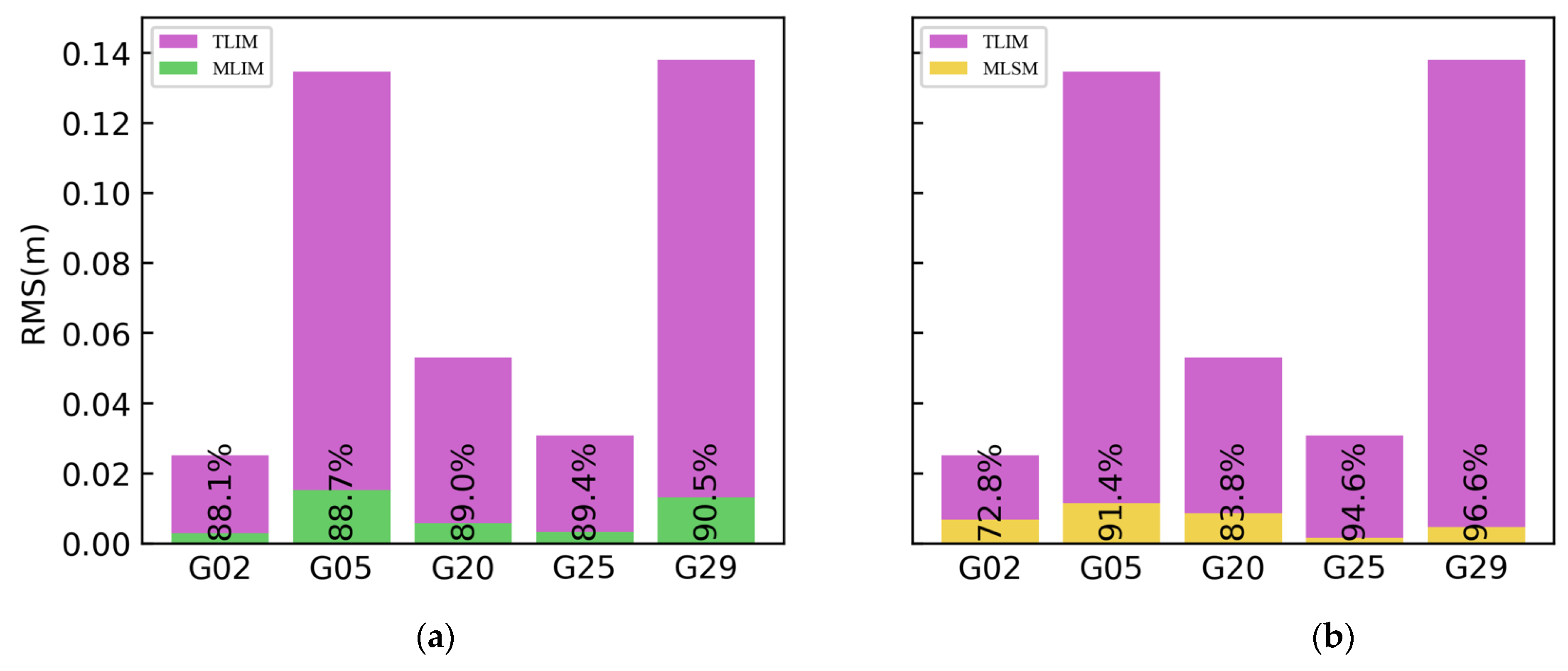
3.2. Comparative Analysis of Different Interpolation Methods

We chose different satellites with different elevation angle changes from the two datasets in order to compare their interpolated tropospheric delays during a certain time period. We also calculated the root mean square (RMS) improvement ratio of several satellites that apply various interpolation methods for tropospheric delay. Meanwhile, we analyzed the variation of the tropospheric delay error with the elevation angles of all satellites using different interpolation methods.

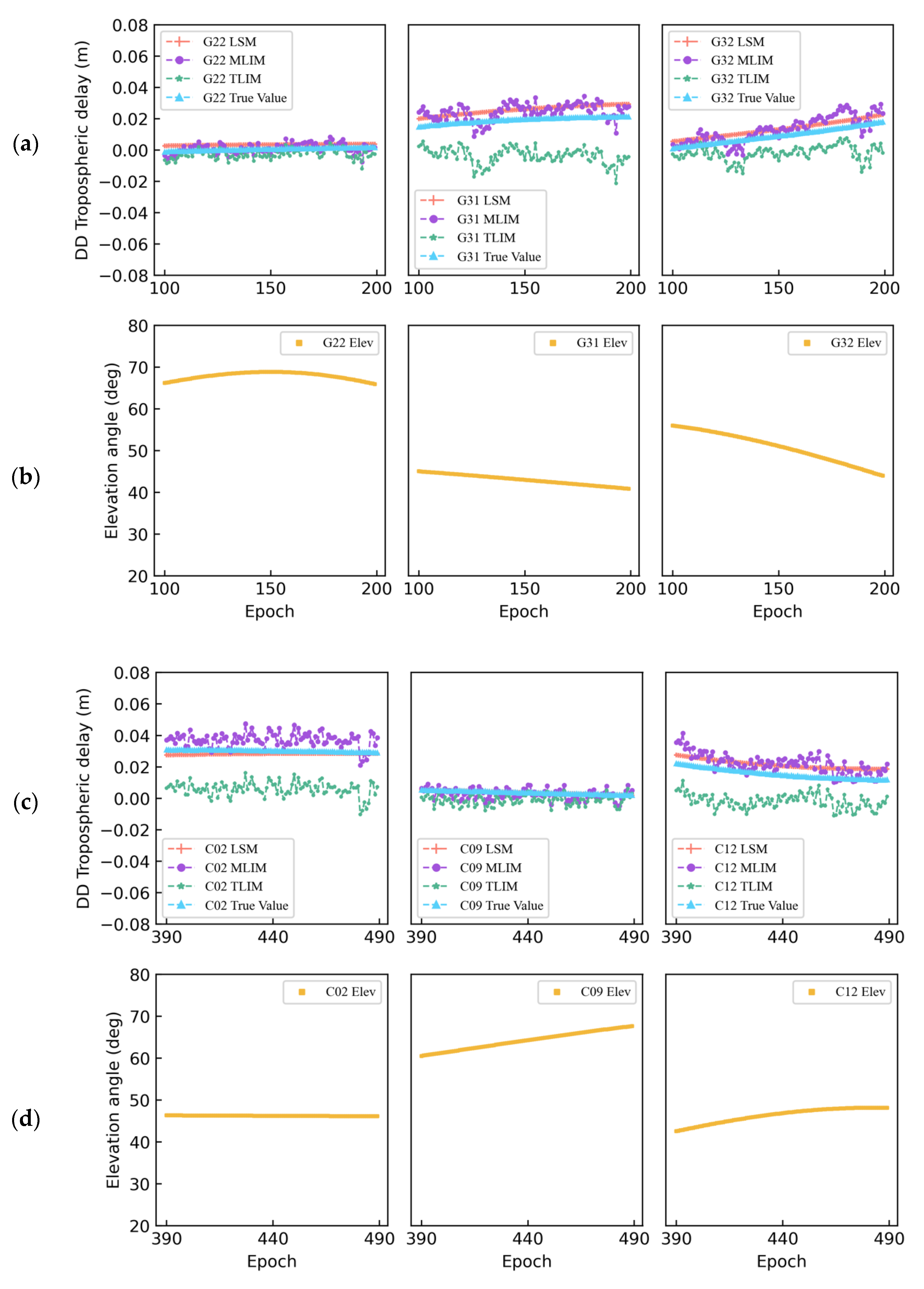
3.2.1. Tropospheric Delay Interpolation Analysis for Dataset 1

Considering the receiver in dataset 1 includes only GPS observations, three continuously observed GPS satellites with different elevation variations during the same period were selected for analysis. The elevation angles and interpolated tropospheric delays were obtained by different methods and exhibited various trends. The results were obtained using traditional LIM, modified LIM, and modified LSM, which are denoted here as TLIM, MLIM, and MLSM, respectively. Figure 4 shows that, in general, as the satellite elevation angle increases, the tropospheric delay decreases, and vice versa. The three GPS satellites can be divided into a low-elevation-angle satellite G05, medium-elevation-angle satellite G29, and high-elevation-angle satellite G02. For all satellites, the DD tropospheric delay obtained by the TLIM interpolation method was found to be quite different from the true value, regardless of whether the satellite elevation angle was rising, falling, or changing slowly. There was a clear offset between TLIM and the true value. The largest disparity between TLIM and the real value was observed for G02, G05, and G20 when their elevation angles were the lowest at approximately 0.05, 0.11, and 0.06 m, respectively. However, no matter how the elevation angles of the three satellites changed, the tropospheric delay interpolated by MLIM and MLSM was almost consistent with the true value. Moreover, the change trend of the interpolated results was nearly identical with the true value.

Figure 5 depicts the RMS statistical results of tropospheric delays for several satellites calculated by different methods. We mainly calculated the increased RMS ratio of MLIM and MLSM compared with TLIM. Overall, the RMS of the MLIM and MLSM methods was found to be much smaller than that of the TLIM, suggesting that the proposed methods improved the accuracy of tropospheric delay interpolation. Among them, MLIM and MLSM presented more noticeable RMS improvements than TLIM on the G29 satellite, with 90.5% and 96.6% improvements, respectively. The average RMS improvement ratio of MLIM and MLSM was 89.1% and 87.8%, respectively, compared to TLIM.

We next analyzed the variation trend of the tropospheric interpolation accuracy of all satellites along with the elevation angles in the selected time period. Figure 6 shows the interpolated tropospheric delay errors under the three methods with the satellite elevation angles. Here, the interpolation accuracy of TLIM increases as the satellite elevation angle increases. However, the interpolation accuracy of MLIM and MLSM consistently maintained high accuracy and seldom fluctuated under satellite elevation changes. In terms of mean errors, TLIM was 0.08 m, whereas MLIM and MLSM were −0.007 and −0.008 m, respectively. The corresponding standard deviations (STD) of the three methods were 0.063, 0.006, and 0.012 m, which indicate that MLIM and MLSM were more stable.

3.2.2. Tropospheric Delay Interpolation Analysis for Dataset 2

Since dataset 2 contains GPS and BDS satellites, we analyzed the tropospheric delays obtained by different interpolation methods for satellites in the two systems, and the results are shown in Figure 7. For GPS satellites, as shown in the results for G22, the DD tropospheric delays by three interpolation methods were consistent with the true values due to the higher elevation angle. However, the satellite elevation angles for G31 and G32 exhibited a declining trend. With the satellite elevation angle decreases, the result of TLIM deviates greatly from the true value, while MLIM and MLSM are closer to the true value. These results indicate an obvious error gap between the results acquired through the TLIM and the true value, whereas the results obtained using the MLIM and MLSM methods were extremely close to the true value and eliminated the systematic errors that occurred under the TLIM. For example, for G31 and G32, the largest offset between TLIM and the true values reached 0.04 and 0.03 m, respectively. However, the differences between MLIM or MLSM and the true values remained within 0.01 m. We also compared three different types of BDS satellites: C02 (Geostationary Orbit, GEO), C09 (Inclined Geosynchronous Orbit, IGSO), and C12 (Middle Earth Orbit, MEO). As shown in Figure 7, since C02 is a GEO satellite, its orbit is geostationary; thus, its elevation angle remains almost constant. However, the tropospheric interpolation results obtained by TLIM significantly depart from the true value, and the maximum deviation reaches 0.05 m. Conversely, the interpolated values obtained by MLIM and MLSM appear nearly identical to the true value. The IGSO satellite C09 had higher elevation angles, and the interpolation results of the three methods were congruent with the true value. For the MEO satellite C12, a model error between the TLIM and the true values was still present, whereas the MLIM and MLSM results were very consistent with the true values.

Similarly, for all satellites in the selected period, we calculated the RMS and improvement ratios of the tropospheric delays interpolated using MLIM and MLSM relative to the TLIM. The results are shown in Figure 8. Here, the largest improvements under MLIM and MLSM compared to TLIM among GPS satellites were observed for G22, with values of 42.1% and 82.4%, respectively. The average improvements under MLIM and MLSM were observed to be 34.3% and 71.4%, respectively. Overall, the improvements under MLSM were more obvious than those under MLIM. Among the BDS satellites, C02 presented the greatest improvements under MLIM and MLSM compared to TLIM, reaching 75.7% and 98.4%, respectively. The average improvements under MLIM and MLSM for BDS satellites were 46.2% and 77.0%, respectively. Thus, the overall improvement effect of MLSM was significantly higher under MLIM.

The tropospheric interpolation errors with the elevation angle changes for the GPS satellites and BDS satellites in dataset 2 using different methods are shown in Figure 9. Here, since all GPS satellites are MEO satellites, the elevation angles of all satellites are constantly changing over the time period, leading the interpolation error results to change continuously. Comparing the mean and standard deviation (STD) of the errors obtained using the three methods, TLIM and MLIM were 0.025 and 0.015 m, respectively, while the MLSM results were −0.006 and 0.006 m. The MLIM and MLSM results were much better than those under TLIM, with MLSM offering a greater improvement effect than TLIM. For BDS satellites, since the BDS contains GEO satellites, the elevation angles of these satellites remained almost unchanged. Hence, the errors of these satellites in the figure vary vertically. The discontinuous part of the figure was caused by the satellite not being in the corresponding range of the elevation angle. It can also be seen that the mean error and STD of the three methods were 0.019 and 0.017 m for TLIM, −0.007 and 0.008 m for MLIM, and −0.005 and 0.008 m for MLSM. MLSM offered the most accurate improvement effect, MLIM was second, and TLIM was worst.

3.3. Comparison of the Positioning Results for Different Interpolation Methods

This section analyzes the positioning performance of the rovers from the two datasets employing VRS. The VRS observations were derived from interpolated ionospheric delay and tropospheric delay via TLIM, MLIM, and MLSM. We evaluated the RMS errors of the positioning results.

Table 1. GPS Positioning RMS statistical results for the rover station in dataset 1.

Dataset 1	E (cm)	N (cm)	U (cm)
TLIM	5.4	5.9	40.9
MLIM	1.1	1.6	5.1
MLSM	1.6	1.8	5.1

to

Table 2. GPS and BDS Positioning RMS statistical results for the rover station in dataset 2.

System	Method	E (cm)	N (cm)	U (cm)
GPS	TLIM	1.0	1.4	14.6
	MLIM	1.0	1.0	6.8
	MLSM	1.3	1.3	3.9
BDS	TLIM	0.6	0.7	11.3
	MLIM	0.4	0.7	4.2
	MLSM	0.6	1.0	2.9

provide the RMS values of the simulated user station positions in datasets 1 and 2, in which the VRS observations generated by various interpolation methods were employed for positioning experiments.

As shown in Table 1, the accuracy of MLIM and MLSM was improved in three directions when compared to TLIM. However, the improvement in the horizontal direction was not noticeable, while the accuracy in the up-component showed remarkable improvements. In the up-component, both MLIM and MLSM improved by 87.5% over TLIM. Table 2 demonstrate the positioning RMS statistics of GPS and BDS in dataset 2. MLIM and MLSM clearly outperformed TLIM in the up-component when utilizing GPS or BDS. The MLIM and MLSM is improved by 58.1% and 73.8% on average in the up-component compared to the TLIM. Regardless of the method utilized, BDS provided slightly greater positioning accuracy than GPS since it has a larger number of visible satellites in the Asia-Pacific region, as depicted in Figure 10. The inclusion of more observational data is advantageous for positioning.

4. Discussion

When there is a height difference between the reference station and the VRS or user station in NRTK, the classical LIM ignores the elevation difference between the measurement stations, leading to non-negligible systematic biases in the interpolated troposphere delays under this method. The user’s positioning accuracy will then decrease, especially in the up-component. In this study, considering the influence of height differences combined with previous studies, we proposed using the MLIM and MLSM methods for NRTK tropospheric delay region modeling. Experiments with two real GNSS datasets from CORS stations demonstrated that MLIM and MLSM improved tropospheric modeling accuracy by an average of 56.5% and 78.7%, respectively, compared to classical LIM. Simultaneously, due to the significant correlation between tropospheric delay and height, the positioning performance of MLIM and MLSM was also improved, particularly in the height direction.

In general, a traditional Delaunay triangulated network (DTN) places a user or VRS in a triangle network surrounded by three CORS stations. In this triangle net, only two independent atmospheric delays can be used for atmosphere modeling. Thus, classical LIM, LCM, or DIM is commonly employed for interpolating tropospheric delays [5,6,7,8,9,10,11,12]. However, these modeling techniques are all implemented on the plane and do not account for the error induced by the altitude factor to the tropospheric correction when there is a considerable height difference between the reference stations. Moreover, the introduction of extra CORS stations not only violates the principles of DTN but also increases the server’s baseline calculation burden, which is insufficient for practical applications. Consequently, we used an a priori tropospheric model, the UNB3m, in combination with approximated coordinates to offer extra tropospheric delay information. Compared to conventional solution methods, this idea has made significant improvement in MLIM and MLSM. In the future, these two improved methods can match the convenience of implementation as well as the real-time and rapid requirements.

It should be noted that this study analyzed the effects of DD tropospheric delay interpolation in NRTK only under notable height differences between the reference station and rover. Future studies should focus on investigating how the DD tropospheric interpolation accuracy is impacted by the spatial distance and height difference between the user and CORS stations in NRTK. Furthermore, as with wide-area PPP, exponential models that more accurately represent the actual variation of tropospheric delays also require further study.

5. Conclusions

This paper presented two modified methods for obtaining the tropospheric corrections in NRTK positioning over complex terrains. Using two regional GNSS networks with obvious height disparities, the performance of the two new methods were analyzed and compared with the conventional method. The conclusions are as follows. Applying MLIM and MLSM will eliminate the systematic errors in the troposphere caused by the height difference and improve the accuracy of tropospheric delay interpolation.

Compared to TLIM, MLIM and MLSM effectively increased the accuracy of tropospheric interpolation for GPS satellites and the three types of satellites (GEO, IGSO, and MEO) in the BDS system, particularly for low-elevation satellites. The DD tropospheric delay interpolation accuracy obtained by the new MLIM and MLSM is improved by 56.5% and 78.7% on average in the two experiments compared to the conventional method.

For the positioning results at the simulated user station, TLIM did not consider the tropospheric errors caused by a height difference, which resulted in errors in the generated VRS observations. These incorrect observations affected the positioning accuracy of the rover and introduced errors to the up-component accuracy. After utilizing MLIM and MLSM, the positioning accuracy of the two data sets in three directions was improved. Especially in the up-component, MLIM and MLSM have an average improvement of 72.8% and 80.7% over TLIM, respectively.

In summary, the proposed two new methods significantly improve the accuracy of tropospheric delay interpolation and positioning performance in the NRTK positioning.

Further research should be carried out to investigate a more effective and comprehensive tropospheric delay modeling method for a larger network of reference stations, in order to contribute to regional atmospheric monitoring.

References

1. Wanninger, L. Virtual reference stations (VRS). GPS Solut. 2003, 7, 143–144. [Google Scholar] [CrossRef]
2. Hu, G.R.; Khoo, H.S.; Goh, P.C.; Law, C.L. Development and assessment of GPS virtual reference stations for RTK positioning. J. Geod. 2003, 77, 292–302. [Google Scholar] [CrossRef]
3. Chen, X.; Han, S.; Rizos, C.; Goh, P.C. Improving real time positioning efficiency using the Singapore integrated multiple reference station network (SIMRSN). In Proceedings of the 13th International Technical Meeting of the Satellite Division of the Institute of Navigation (ION GPS 2000), Salt Lake City, UT, USA, 19–22 September 2000. [Google Scholar]
4. Wanninger, L. Improved ambiguity resolution by regional differential modelling of the ionosphere. In Proceedings of the 8th International Technical Meeting of the Satellite Division of The Institute of Navigation (ION GPS 1995), Palm Springs, CA, USA, 12–15 September 1995. [Google Scholar]
5. Wanninger, L. The performance of virtual reference stations in active geodetic GPS-networks under solar maximum conditions. In Proceedings of the 12th International Technical Meeting of the Satellite Division of The Institute of Navigation (ION GPS 1999), Nashville, TN, USA, 14–17 September 1999. [Google Scholar]
6. Han, S.; Rizos, C. GPS network design and error mitigation for real-time continuous array monitoring systems. In Proceedings of the 9th International Technical Meeting of the Satellite Division of The Institute of Navigation (ION GPS 1996), Kansas City, MO, USA, 17–20 September 1996. [Google Scholar]
7. Gao, Y.; Li, Z.; McLellan, J. Carrier phase based regional area differential GPS for decimeter-level positioning and navigation. In Proceedings of the 10th International Technical Meeting of the Satellite Division of The Institute of Navigation (ION GPS 1997), Kansas City, MO, USA, 16–19 September 1997. [Google Scholar]
8. Wübbena, G.; Bagge, A.; Seeber, G.; Böder, V.; Hankemeier, P. Reducing distance dependent errors for real-time precise DGPS applications by establishing reference station networks. In Proceedings of the ION GPS, Kansas City, MO, USA, 17–19 September 1996. [Google Scholar]
9. Dai, L.; Han, S.; Wang, J.; Rizos, C. Comparison of interpolation algorithms in network-based GPS techniques. Navig. J. Inst. Navig. 2003, 50, 277–293. [Google Scholar] [CrossRef]
10. Fotopoulos, G.; Cannon, M. An overview of multi-reference station methods for cm-level positioning. GPS Solut. 2001, 4, 1–10. [Google Scholar] [CrossRef]
11. Wu, S. Performance of Regional Atmospheric Error Models for NRTK in GPSnet and the Implementation of a NRTK System. Ph.D. Thesis, RMIT University, Melbourne, Australia, 2009. [Google Scholar]
12. Al-Shaery, A.; Lim, S.; Rizos, C. Investigation of different interpolation models used in Network-RTK for the virtual reference station technique. J. Glob. Position Syst. 2011, 10, 136–148. [Google Scholar] [CrossRef] [Green Version]
13. Wielgosz, P.; Cellmer, S.; Rzepecka, Z.; Paziewski, J.; Grejner-Brzezinska, D.A. Troposphere modeling for precise GPS rapid static positioning in mountainous areas. Meas. Sci. Technol. 2011, 22, 045101. [Google Scholar] [CrossRef]
14. Liangke, H.; Lilong, L.; Chaolong, Y. A zenith tropospheric delay correction model based on the regional CORS network. Geod. Geodyn. 2012, 3, 53–62. [Google Scholar] [CrossRef] [Green Version]
15. Yin, H.; Huang, D.; Xiong, Y. Regional tropospheric delay modeling based on GPS reference station network. In Proceedings of the VI Hotine-Marussi Symposium on Theoretical and Computational Geodesy, Wuhan, China, 29 May–2 June 2006. [Google Scholar]
16. Landau, H.; Vollath, U.; Chen, X. Virtual reference stations versus broadcast solutions in network RTK–advantages and limitations. In Proceedings of the GNSS, Graz, Austria, 22–25 April 2003. [Google Scholar]
17. Wu, B.; Gao, C.; Pan, S.; Deng, J.; Gao, W. Regional modeling of atmosphere delay in network rtk based on multiple reference station and precision analysis. In China Satellite Navigation Conference (CSNC) 2015 Proceedings: Volume II; Springer: Berlin/Heidelberg, Germany, 2015. [Google Scholar]
18. Lei, Q.; Lei, L.; Zemin, W. An tropospheric delay model for GPS NET RTK. In Proceedings of the 2010 Second International Conference on Information Technology and Computer Science, Kiev, Ukraine, 24–25 July 2010; IEEE: Piscataway, NJ, USA, 2010. [Google Scholar]
19. Shi, J.; Xu, C.; Guo, J.; Gao, Y. Local troposphere augmentation for real-time precise point positioning. Earth Planets Space 2014, 66, 30. [Google Scholar] [CrossRef] [Green Version]
20. Zhang, H.; Yuan, Y.; Li, W.; Zhang, B.; Ou, J. A grid-based tropospheric product for China using a GNSS network. J. Geod. 2018, 92, 765–777. [Google Scholar] [CrossRef]
21. Zheng, F.; Lou, Y.; Gu, S.; Gong, X.; Shi, C. Modeling tropospheric wet delays with national GNSS reference network in China for BeiDou precise point positioning. J. Geod. 2018, 92, 545–560. [Google Scholar] [CrossRef]
22. Zhang, H.; Yuan, Y.; Li, W. Real-time wide-area precise tropospheric corrections (WAPTCs) jointly using GNSS and NWP forecasts for China. J. Geod. 2022, 96, 44. [Google Scholar] [CrossRef]
23. Pu, Y.; Song, M.; Yuan, Y.; Che, T. Triple-frequency ambiguity resolution for GPS/Galileo/BDS between long-baseline network reference stations in different ionospheric regions. GPS Solut. 2022, 26, 146. [Google Scholar] [CrossRef]
24. Hu, G.; Abbey, D.A.; Castleden, N.; Featherstone, W.E.; Earls, C.; Ovstedal, O.; Weihing, D. An approach for instantaneous ambiguity resolution for medium-to long-range multiple reference station networks. GPS Solut. 2005, 9, 1–11. [Google Scholar] [CrossRef]
25. Yuan, Y.; Ou, J. An improvement to ionospheric delay correction for single-frequency GPS users–the APR-I scheme. J. Geod. 2001, 75, 331–336. [Google Scholar] [CrossRef]
26. Klobuchar, J.A. Ionospheric effects on GPS. In Global Positioning System Theory & Applications; American Institute of Aeronautics and Astronautics: Reston, VA, USA, 1991; Volume 1, pp. 517–546. [Google Scholar]
27. Yuan, Y.; Wang, N.; Li, Z.; Huo, X. The BeiDou global broadcast ionospheric delay correction model (BDGIM) and its preliminary performance evaluation results. Navigation 2019, 66, 55–69. [Google Scholar] [CrossRef] [Green Version]
28. Øvstedal, O. Absolute Positioning with Single-Frequency GPS Receivers. GPS Solut. 2002, 5, 33–44. [Google Scholar] [CrossRef]
29. Leandro, R.F.; Langley, R.B.; Santos, M.C. UNB3m_pack: A neutral atmosphere delay package for radiometric space techniques. GPS Solut. 2008, 12, 65–70. [Google Scholar] [CrossRef]
30. Niell, A.E. Global Mapping Functions for the Atmosphere Delay at Radio Wavelengths. J. Geophys. Res. Solid Earth 1996, 101, 3227–3246. [Google Scholar] [CrossRef]
31. Zhang, J.; Lachapelle, G. Precise estimation of residual tropospheric delays using a regional GPS network for real-time kinematic applications. J. Geod. 2001, 75, 255–266. [Google Scholar] [CrossRef]
32. Teunissen, P.J.G. The least-square ambiguity decorrelation adjustment: A method for fast GPS ambiguity estimation. J. Geod. 1995, 70, 65–82. [Google Scholar] [CrossRef]
33. Yao, Y.; Xu, X.; Xu, C.; Peng, W.; Wan, Y. Establishment of a Real-Time Local Tropospheric Fusion Model. Remote Sens. 2019, 11, 1321. [Google Scholar] [CrossRef] [Green Version]
34. Bartels, J. The technique of scaling indices K and Q of geomagnetic activity. Ann. Intern. Geophys. 1957, 4, 215–226. [Google Scholar]
35. Mireault, Y.; Tétreault, P.; Lahaye, F.; Héroux, P.; Kouba, J. Online precise point positioning. GPS World 2008, 19, 59–64. [Google Scholar]
36. Guo, Q. Precision comparison and analysis of four online free PPP services in static positioning and tropospheric delay es-timation. GPS Solut. 2015, 19, 537–544. [Google Scholar] [CrossRef]
37. Xiao, G.; Liu, G.; Ou, J.; Liu, G.; Wang, S.; Guo, A. MG-APP: An open-source software for multi-GNSS precise point positioning and application analysis. GPS Solut. 2020, 24, 66. [Google Scholar] [CrossRef]
38. Xiao, G.; Liu, G.; Ou, J.; Zhou, C.; He, Z.; Chen, R.; Guo, A.; Yang, Z. Real-time carrier observation quality control algorithm for precision orbit determination of LEO satellites. GPS Solut 2022, 26, 102. [Google Scholar] [CrossRef]
39. Liu, S.; Yuan, Y. Generating GPS decoupled clock products for precise point positioning with ambiguity resolution. J. Geod. 2022, 96, 6. [Google Scholar] [CrossRef]
Figure 1. The distribution of experimental dataset 1 stations.
Atmosphere 14 00083 g001
Figure 2. The distribution of experimental dataset 2 stations.
Atmosphere 14 00083 g002
Figure 3. The elevation distribution of the stations in two datasets.
Atmosphere 14 00083 g003
Figure 4. Comparison of the DD tropospheric delay interpolated by different methods (a) and the satellite elevation variation of G02, G05, and G29 (b).
Atmosphere 14 00083 g004
Figure 5. The DD tropospheric delay RMS and improvement ratio obtained by MLIM compared to TLIM (a); the DD tropospheric delay RMS and improvement ratio obtained by MLSM compared to TLIM (b).
Atmosphere 14 00083 g005
Figure 6. Variation trend of DD tropospheric errors for different satellites with a change in elevation calculated by TLIM (a), MLIM (b), and LSM (c).
Atmosphere 14 00083 g006
Figure 7. The satellite elevation angle variation and comparison of the DD tropospheric delay obtained by different methods with the true values for GPS (a,b) and BDS (c,d).
Atmosphere 14 00083 g007
Figure 8. GPS (a,b) and BDS (c,d) satellites using the MLIM, TLIM, and MLSM interpolation methods to obtain the RMS of the DD tropospheric delay and the improvement ratios of MLIM and MLSM.
Atmosphere 14 00083 g008
Figure 9. TLIM (left), MLIM (middle), and MLSM (right) change trend of DD tropospheric errors with changes in elevation angle for GPS satellites (a) and BDS satellites (b).
Atmosphere 14 00083 g009
Figure 10. Number of satellites based on GPS and BDS in dataset 2.
Atmosphere 14 00083 g010