Abstract
Australia experiences a variety of climate extremes that result in loss of life and economic and environmental damage. This paper provides a first evaluation of the performance of state-of-the-art Coupled Model Intercomparison Project Phase 6 (CMIP6) global climate models (GCMs) in simulating climate extremes over Australia. Here, we evaluate how well 37 individual CMIP6 GCMs simulate the spatiotemporal patterns of 12 climate extremes over Australia by comparing the GCMs against gridded observations (Australian Gridded Climate Dataset). This evaluation is crucial for informing, interpreting, and constructing multimodel ensemble future projections of climate extremes over Australia, climate-resilience planning, and GCM selection while conducting exercises like dynamical downscaling via GCMs. We find that temperature extremes (maximum-maximum temperature -TXx, number of summer days -SU, and number of days when maximum temperature is greater than 35 °C -Txge35) are reasonably well-simulated in comparison to precipitation extremes. However, GCMs tend to overestimate (underestimate) minimum (maximum) temperature extremes. GCMs also typically struggle to capture both extremely dry (consecutive dry days -CDD) and wet (99th percentile of precipitation -R99p) precipitation extremes, thus highlighting the underlying uncertainty of GCMs in capturing regional drought and flood conditions. Typically for both precipitation and temperature extremes, UKESM1-0-LL, FGOALS-g3, and GCMs from Met office Hadley Centre (HadGEM3-GC31-MM and HadGEM3-GC31-LL) and NOAA (GFDL-ESM4 and GFDL-CM4) consistently tend to show good performance. Our results also show that GCMs from the same modelling group and GCMs sharing key modelling components tend to have similar biases and thus are not highly independent.
1. Introduction
Climate extremes threaten human health, economic stability, and the well-being of natural and built environments. As the world continues to warm, climate hazards are expected to increase in frequency and intensity [1]. Climate extremes have increased on all continents since 1980, most notably in Australia, and this has dramatically impacted human life, economy and environment [2,3,4,5]. Zander et al. (2015) [6] showed that heat-related extremes during 2013–2014 led to an annual economic burden of around US$6.2 billion (95% CI: 5.2–7.3 billion) for the Australian workforce. This amounts to 0.33 to 0.47% of Australia’s GDP (Gross Domestic Product).
Australia is exposed to various climates due to its large size and meridional extent. With such a wide range of climates, Australia also experiences a great diversity of climatic extremes [2,5,7]. Australia regularly experiences extremes in precipitation and temperature: from severe droughts to intense precipitation [8,9,10,11,12,13] and from increases in hot extremes and decreases in cold extremes [14,15,16]. These extremes have a substantial impact on Australia’s unique flora and fauna [17], agriculture [18], urban infrastructure [19], and human health [20]. Thus, it is crucial to examine the simulated extremes in Australia’s present-day and future climate, as it is for other regions. This interpretation is an important aspect of adaptation planning, as changes to rare but high-impact climate extremes are likely to be a greater challenge to communities compared to changes in the mean climate state.
Global climate models (GCMs) have been used as a primary tool for examining the past and future changes in climate extremes at global and continental scales [21,22,23,24,25]. Several studies have conducted comprehensive reviews of projected changes in climate extremes globally and regionally based on the different phases of the Coupled Modelling Intercomparison Project (CMIP) [26,27,28]. Recently, the latest iteration of CMIP, phase 6 (CMIP6) [29], has been released, which provides new opportunities to examine the climate system and make regional projections via downscaling. Compared to CMIP5 [30], the models in CMIP6 generally have finer model resolution and improved physical processes [31]. One of the focuses of CMIP6 is assessing climate extremes changes and understanding associated physical processes [29].
Several studies have already evaluated the performance of CMIP6 GCMs in simulating extremes globally and over different regions of the world. However, most of these studies have evaluated how the multimodel ensemble of CMIP6 performs in comparison to the multimodel ensemble of CMIP5 (for example, Grose et al. 2020 [32], Di Virgilio et al. 2022 [33] and Deng et al. 2021 [34] over Australia; Masud et al. 2021 [35] over Canada; Gusain et al. 2020 [36] over India; Akinsanola et al. 2021 [37] over Eastern Africa; Ukkola et al. 2020 [38] and Seneviratne & Hauser 2020 [39] globally). Most of these studies have concluded that the CMIP6 GCM ensemble offers marginal improvements versus the CMIP5 ensemble in terms of capturing observed climate extremes. These studies assist in understanding how GCM ensembles perform in simulating climate extremes; however, to understand the physical processes driving modelled climate extremes, knowledge of the performances of individual GCMs is needed. Assessment of the performance of individual GCMs in resolving climate extremes also assists with the selection of GCMs for regional dynamical downscaling [40,41] and for assessing the potential impacts of extreme events on biophysical and socio-economic systems [42].
There have been a few studies that have looked at the performance of individual CMIP6 GCMs in capturing observed climate extremes over different parts of the globe: for example, the United States [43], southeast Asia [44], China and Western North Pacific and East Asia [45]. Over Australia, Di Virgilio et al. 2022 [33] evaluated CMIP6 GCMs for climate extremes; however, their study was only limited to percentile-based temperature and precipitation extremes. Understanding the relative performances of CMIP6 GCMs in simulating climate extremes over Australia is of direct relevance to multiple stakeholders, such as researchers and climate impact resilience planners, as GCMs can show a wide variety of inter-model differences in performance.
Therefore, the aims of this study are: 1. To evaluate how well individual CMIP6 GCMs perform in terms of capturing precipitation and temperature extremes over Australia. 2. To find the subset of best performing CMIP6 GCMs for capturing these climate extremes. 3. To assess if the GCM performance varies for continental Australia and sub-regions across Australia with different topography and climate.
2. Data and Methods
2.1. CMIP6 GCMs
This study uses one simulation each from a group of 37 CMIP6 GCMs that are available at the time of writing. Out of 37 CMIP6 GCMs, some GCMs are from the same parent institute and share modelling components such as GCMs from Australian Community, whereas some GCMs just use different resolutions such as MPI-ESM1-2-HR and MPI-ESM1-2-LR. The spatial resolution of the GCMs varies (Table 1). To compare the GCMs with the observations, we re-grid all 37 GCMs to the most common resolution of 1.5° × 1.5° on a regular lat/lon grid using conservative re-gridding. We acknowledge that re-gridding coarser resolution models onto a higher resolution has limitations [46]; however, going to any coarser resolution than 1.5° × 1.5° would lead to fewer grid points in the domain and thus affect the robustness of the analysis. In addition, past studies have also used similar re-gridding models to the most common resolution when analysing datasets like CMIP5 and CMIP6 [32,33]. We chose the most common present-day period between GCMs, i.e., 1951–2014, for the evaluation. The reason for choosing a longer period (64 years) is to minimize inter-annual variations.

Table 1.
CMIP6 Models and simulations used in this study. Here colours other than black denote GCMs from the same modelling institution.
While extreme climate and weather events are generally multifaceted phenomena, in this study, we evaluate climate extremes based on daily precipitation and temperature as defined by the Expert Team on Sector-specific Climate Indices (ET-SCI; [47,48]. We use the ClimPACT version 2 software to calculate the ET-SCI indices (https://climpact-sci.org/ accessed on 1 November 2020), focusing on daily precipitation, maximum temperature, and minimum temperature.
Although ClimPACT produces 34 core indices (more than 80 indices in total), we use 12 indices based on the following considerations. 1. To capture key aspects of climate extremes; for example, we choose absolute indices (e.g., maximum 1-day precipitation (Rx1day), hottest day (TXx), coldest day (TNn)), threshold-based indices (e.g., number of heavy rain days (R10mm), tropical nights, i.e., the annual count of days when daily minimum temperature > 20 °C (TR), summer days, i.e., the annual count of days when daily maximum temperature > 25 °C (SU), number of days when maximum temperature is greater than 35 °C (TXge35)), percentile indices (e.g., total annual precipitation from very heavy rain days (R99p)), and duration indices (e.g., consecutive wet days (CWD), consecutive dry days (CDD), warm spell duration index (WSDI), cold spell duration index (CSDI). 2. To capture extremes which have an impact on society and infrastructure; for example, extreme indices like TXge35, TR, and SU have the largest impacts on health [49], whereas indices like Rx1day, CDD, and CWD have the largest impact on agriculture, water resources and the economy [50,51].
2.2. Observations
We use observational data from the Australian Gridded Climate Dataset (AGCD Evans et al. 2020 [52]) to compare the CMIP6 GCM simulated extremes with observations for the present-day period. AGCD data have a spatial resolution of 0.05° × 0.05° and are obtained from an interpolation of station observations across the Australian continent. Most of these stations are in the more heavily populated coastal areas with a sparser representation inland over central Australia. Taking the same approach as for the GCMs, we re-grid the AGCD data to a common resolution of 1.5° × 1.5° and then calculate the ET-SCI indices using ClimPACT.
Since AGCD observations are only available for land, in this study, we evaluate CMIP6 GCMs only for grids over land. Due to the sparse distribution of precipitation gauges in central Australia, this region has no quality gridded observations available [53]. Therefore, we mask both ocean and parts of central Australia to examine precipitation extremes.
2.3. Methodology
Several studies have proposed multiple metrics for evaluating climate models. The metrics range from summarising features of the spatial distribution of the climatological mean state to summarising the temporal variability [54,55,56,57]. Some of the common and widely used metrics for evaluating the spatial climatology distribution of models against observations are biased (difference between the modelled and observed climatological mean field; here, smaller values indicate better performance of the model simulation), root mean square error (RMSE: square root of the difference between the modelled and observed climatological mean field; here smaller values indicate better performance of the model simulation) and pattern correlation (PCorr: correlation between the modelled and observed climatological mean field; Equation (1); Benesty et al. 2009 [58]). Here and denote the values of the variable in a sample of model simulations and the observational data sets, respectively, whereas and denote the means of the variable in a sample of model simulations and the observational data sets, respectively. Here, larger PCorr values indicate better performance of the model simulation.
For analysing the performance of the models with respect to temporal variation, studies have proposed the evaluation of interannual variability score (IVS, Equation (2); Chen et al. 2011 [59]; Fan et al. 2020 [60]). Here STDm and STDo denote the interannual standard deviation of the model simulations and the observational data sets, respectively. This score analyses the performance of models with respect to temporal variation and suggests how well the models can reproduce the temporal standard deviation. Smaller IVS values indicate better performance of the model simulation.
For each extreme index mentioned in Table 2, we calculate all the above-mentioned metrics, i.e., bias, RMSE, PCorr and IVS, to determine the performance of GCMs in capturing the observed extremes.
Table 2.
List of ET-SCI Indices evaluated in this study.
Not all metrics are independent, and some metrics will inevitably be correlated with others. Still, the effort has been made to include roughly the same number of metrics from each variable, minimizing this issue. Once performance metrics are calculated (i.e., biases, spatial RMSEs, spatial correlations, IVS score for each variable/statistic and for each timescale), these are normalized following Rupp et al. 2013 [54], as per Equation (3);
where Ei,j is an error for a given model i and metric j. Note that for correlations, each min () or max () function in Equation (1) is reversed. The relative error is then summed across all m metrics following Rupp et al. (2013), as per Equation (4):
3. Results
We evaluate indices for either monthly or annual periods (Table 2). For the annual indices, evaluation metrics (bias, RMSE, Pcorr and IVS) are only calculated at the annual timescale, whereas for the monthly indices, the evaluation metrics are calculated at both the annual and seasonal (December-January-February (DJF), March-April-May (MAM), June-July-August (JJA) and September-°October-November (SON)) timescales. Due to space limitations, we only show the biases at the annual scale in the main text. The biases at the seasonal scale are provided in the Supplementary Materials.
3.1. Climatology of Indices
3.1.1. Precipitation Extremes
Figure 1, Figure 2, Figure 3, Figure 4 and Figure 5 show the observed climatological mean and biases in individual CMIP6 GCMs for annual R99p, Rx1day, R10mm, CWD, and CDD, respectively. When assessing biases, we calculate the statistical significance of bias for each grid cell using t-tests (α = 0.05) and Mann–Whitney U test for temperature and precipitation-based extremes, respectively. Stippling shows statistically significant bias.
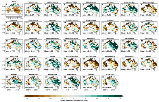
Figure 1.
Climatological mean annual bias in total annual precipitation from very heavy rain days (R99p: mm) relative to the Australian Gridded Climate Data dataset (AGCD; panel 1) for the individual CMIP6 GCMs (panels 2–38). Data spans 1951—2014. Stippling indicates statistically significant differences using a student’s t-test at the 95% confidence level. The white masks in part of the inland domain are the regions with no station data.
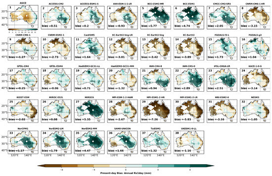
Figure 2.
Climatological mean annual bias in maximum 1-day precipitation (Rx1Day: mm) relative to the Australian Gridded Climate Data dataset (AGCD; panel 1) for the individual CMIP6 GCMs (panels 2–38). Data spans 1951–2014. Stippling indicates statistically significant differences using a student’s t-test at the 95% confidence level. The white masks in part of the inland domain are the regions with no station data.
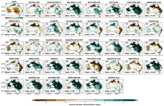
Figure 3.
Climatological mean annual bias in the number of very heavy rain days (rain > 10 mm) (R10mm: days) relative to the Australian Gridded Climate Data dataset (AGCD; panel 1) for the individual CMIP6 GCMs (panels 2–38). Data spans 1951–2014. Stippling indicates statistically significant differences using a student’s t-test at the 95% confidence level. The white masks in part of the inland domain are the regions with no station data.
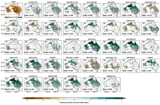
Figure 4.
Climatological mean annual bias in consecutive wet days (CWD: days) relative to the Australian Gridded Climate Data dataset (AGCD; panel 1) for the individual CMIP6 GCMs (panels 2–38). Data spans 1951–2014. Stippling indicates statistically significant differences using a student’s t-test at the 95% confidence level. The white masks in part of the inland domain are the regions with no station data.
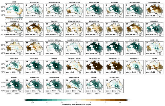
Figure 5.
Climatological mean annual bias in consecutive dry days (CDD: days) relative to the Australian Gridded Climate Data dataset (AGCD; panel 1) for the individual CMIP6 GCMs (panels 2–38). Data spans 1951–2014. Stippling indicates statistically significant differences using a student’s t-test at the 95% confidence level. The white masks in part of the inland domain are the regions with no station data.
The spatial distribution of biases in R99p and Rx1day (Figure 1 and Figure 2) look similar to each other. The majority of GCMS show the largest bias in the eastern half of Australia for both extremes. For R99p, TaiESM1 shows the least bias of 0.4 mm, and MPI-ESM1-1-HR and BCC-CSM2-MR show the maximum dry and wet bias of 40.2 and 36.1 mm, respectively. HadGEM3-GC31-MM, INM-CM4-8, TaiESM1, KIOST-ESM, ACCESS-CM2, FGOALS-f3-L and FGOALS-f3 show lower biases, whereas BCC-CSM2-MR and INM-CM5-0 show higher wet bias and CNRM-CM6-1-HR, MPI-ESM-1-2-HAM, MPI-ESM1-2-HR and MPI-ESM1-2LR (MPI Germany) show the highest dry bias respectively (Table 3).
Table 3.
Table of continentally averaged absolute bias recorded in 37 CMIP6 GCMs for the 12 extreme indices. A smaller value of bias corresponds to the better performance of GCMs. Here, the colour green and red denote the best (top 25% subset) and worst (bottom 25% subset) performing GCMs.
For Rx1day, GCMs typically show absolute mean biases in the range of 0.1 mm (MIR°C-ES2L) and 7.3 mm (MPI-ESM1-2-HR). Here, ACCESS-CM2, ACCESS-ESM1-5 (Australian Community), AWI-ESM-1-1-LR, FGOALS-g3, HadGEM3-GC31-LL, INM-CM4-8, GFDL-ESM4 and GFDL-CM4 (NOAA) show the lowest bias whereas BCC-CSM2-MR, BCC-ESM1 (Beijing Climate Centre), MPI-ESM1-2-HR, MPI-ESM1-2LR, MIR°C6, NorESM2-MM, EC-Earth3-Veg and EC-Earth3 (EC-Earth Consortium) show the largest bias (~ 4–7 mm) (Table 3) both wet and dry.
For both R99p and Rx1day, there are two subsets of GCMs showing greater dry bias (EC-Earth-Veg-LR, EC-Earth3-Veg and EC-Earth3 (EC-Earth Consortium), MPI-ESM-1-2-HAM, MPI-ESM1-2-HR and MPI-ESM1-2-LR (MPI-Germany)) and wet bias (BCC-CSM2-MR and BCC-ESM1 (Beijing Climate Centre), INM-CM4-8 and INM-CM5-0 (INM Russia)).
For R10mm (Figure 3), ACCESS-CM2, ACCESS-ESM1-5 (Australian Community), BCC-CSM2-MR, CNRM-CM6-1, FGOALS-g3, GFDL-ESM4, HadGEM3-GC31-LL show the smallest wet bias whereas AWI-ESM-1-1-LR, CMCC-CM2-SR5, IPSL-CM6A-LR, MPI-ESM-1-2-HAM, MPI-ESM1-2-HR, NESM3, NorCPM1, NorESM2-MM and SAM0-UNICON show the largest wet bias. Like R99p and Rx1day, GCMs for R10mm also show greater bias in eastern Australia than elsewhere.
For CDD and CWD (Figure 4 and Figure 5), GCMs do not show large spatial variation in the sign of the bias. In addition to this, the GCMs with dry and wet biases in R99p and Rx1day overestimate (CDD) and underestimate (CWD) consecutive days, respectively. For CWD, GCMs typically show a small bias (between 0.5–2.5 days); however, there are outlier GCMs (INM-CM4-8 and NorCPM1) which show biases greater than 3 days. Here, ACCESS-CM2, GFDL-ESM4, GFDL-CM4 (NOAA), HadGEM3-GC31-LL and HadGEM3-GC31-MM (Hadley Centre) are found to be top performers (top 25% subset). In addition, CNRM-CM6-1, KACE-1-0-G, MRI-ESM2-0 and UKESM1-0-LL also show small biases and are among the top performers. For CDD, GCMs typically show a very strong bias (between 4–10 days) compared to CWD. Outlier GCMs show bias greater than 10 days; for example, MPI-ESM1-2-HR show the strongest bias of 30.3 days, whereas INM-CM4-8 and INM-CM5-0 (INM Russia) show biases greater than 15 days.
The large biases in CDD for GCMs from CNRM, INM Russia, MPI Germany, and National Institute for Environmental Studies Japan suggest that some GCMs typically struggle to capture the CDD. This can be attributed to the drizzle problem in GCMs. Past studies have suggested that convective precipitation generated by the cumulus parameterisation in coarse resolution GCMs is too frequent and long-lasting with reduced intensity, leading to the “drizzling” bias [61]. The drizzling bias impedes realistic representation of precipitation extremes like CDD and results in a large bias.
Spatial maps of biases at seasonal timescales for Rx1day (Figures S1–S4), R10mm (Figures S5–S8), CWD (Figures S9–S12) and CDD (Figures S13–S16) are provided in the Supplementary Material. A comparison of seasonal biases showed a similar story as the annual biases for all the precipitation extremes, i.e., GCMs with annual dry and wet biases demonstrate similar seasonal dry and wet biases, and those biases have similar spatial distributions.
We observe that models from the same parent institution tend to have similar biases for precipitation extremes (i.e., in terms of spatial structure, sign and magnitude). For example, both GCMs from the Beijing Climate Centre: BCC-CSM2-MR and BCC-ESM1, show wet biases in most parts of the continent. Similarly, GCMs from Norwegian Climate Centre: NorCPM1, NorESM2-LM and NorESM2-MM and GCMs from INM Russia: INM-CM4-8 and INM-CM5-0 also have wet biases over most parts of Australia. The GCMs from MPI Germany: MPI-ESM-1-2-HAM, MPI-ESM1-2-HR, and MPI-ESM1-2-LR, respectively, show dry biases across the continent. We note that GCMs from the same parent institution often share key modelling components such as land-surface components, atmospheric and °Ocean models and are thus not highly independent of each other.
Although GCMs from the same parent institution can show large inter-model similarity, GCMs from the Chinese Academy of Sciences appear more independent. Here, FGOALS-f3-L shows dry bias, whereas FGOALS-g3 shows wet bias for most precipitation indices except for Rx1day. After investigating details about the model configurations, we found that both these GCMs have substantial differences in their components. For example, FGOALS-f3-L is a fully coupled climate system model consisting of four component models, whereas FGOALS-g3 comprises five components [62]. In FGOALS-f3-L, all the component models are coupled via the NCAR Coupler 7 [63], whereas, in FGOALS-g3, all the component models are coupled via Community Coupler, version 2 (C-Coupler2), developed by Tsinghua University [64]. These differences between the modelling components of these two GCMs are likely the reason for their dissimilarity.
Typically, for most precipitation extremes, the GCMs which show large bias also show large RMSE. At the annual timescale, for Rx1day and R99p, CNRM-CM6-1-HR, MPI-ESM-1-2-HAM, NESM3, and EC-Earth3-Veg-LR show the smallest RMSE, whereas BCC-CSM2-MR, BCC-ESM1 (Beijing Climate Centre), CanESM5, FGOALS-f3-L, INM-CM5-0, MIR°C6 and NorESM2-MM show the largest RMSE (Table 4). For R10mm and CWD, HadGEM3-GC31-LL, HadGEM3-GC31-MM (Hadley Centre), GFDL-ESM4, GFDL-CM4 (NOAA), and UKESM1-0-LL show the smallest RMSE whereas SAM0-UNICON, NorCPM1, IPSL-CM6A-LR and CMCC-CM2-SR5 show the largest RMSE.
Table 4.
Table of continentally averaged root mean square error (RMSE) recorded in 37 CMIP6 GCMs for the 12 extreme indices. A smaller value of RMSE corresponds to the better performance of GCMs. Here, the colour green and red denote the best (top 25% subset) and worst (bottom 25% subset) performing GCMs.
For CDD, MPI-ESM1-2-HR and MPI-ESM1-2-LR (MPI Germany) show the largest RMSE, whereas HadGEM3-GC31-LL, HadGEM3-GC31-MM (Hadley Centre), UKESM1-0-LL, ACCESS-CM2 and ACCESS-ESM1-5 (Australian Community) show the smallest RMSE (Table 4).
For PCorr and IVS (Table 5 and Table 6), GCMs show approximately similar results to the bias and RMSE evaluation, i.e., GCMs which show low bias and RMSE also capture spatial (have high Pcorr) and temporal patterns (have low IVS score) well, like HadGEM3-GC31-LL, HadGEM3-GC31-MM, GFDL-ESM4, GFDL-CM4 and UKESM1-0-LL. There are also exceptions to this pattern. For example, EC-Earth-Veg-LR, EC-Earth3-Veg and EC-Earth3 (EC-EARTH Consortium) show top and average performance for PCorr and IVS, respectively, but they are not always in the top performing models for bias and RMSEs for most indices.
Table 5.
Table of pattern correlation (PCorr) recorded in 37 CMIP6 GCMs for the 12 extreme indices. A larger value of PCorr corresponds to the better performance of GCMs. Here, the colour green and red denote the best (top 25% subset) and worst (bottom 25% subset) performing GCMs.
Table 6.
Table of interannual variability score (IVS) recorded in 37 CMIP6 GCMs for the 12 extreme indices. A smaller value of IVS corresponds to the better performance of GCMs. Here, the colour green and red denote the best (top 25% subset) and worst (bottom 25% subset) performing GCMs.
3.1.2. Temperature Extremes
Figure 6, Figure 7, Figure 8, Figure 9, Figure 10, Figure 11 and Figure 12 show the observed annual climatological mean and biases in CMIP6 GCMs for TXx, TXge35, SU, TNn, TR, WSDI and CSDI, respectively. On average, most GCMs typically show cold biases for hot extremes and warm biases for cold extremes, except for WSDI and CSDI. However, the magnitude of bias for cold extremes is generally larger than that of hot extremes. There also exists an exception to this pattern. For example, CanESM5, KIOST-ESM, MIR°C-ES2L, MIR°C6 and MRO-ESM2-0 show strong hot bias for hot extremes, whereas GFDL-CM4, USESM1-0-LL and NorCPM1 show slight cold bias for cold extremes. In addition, GCMs which struggle to capture the extremes of maximum temperature also perform poorly in capturing extremes of minimum temperature.
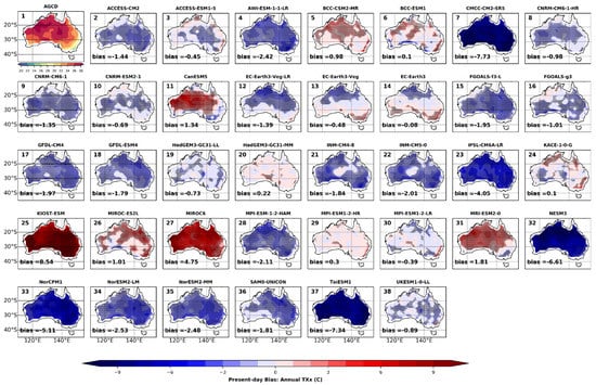
Figure 6.
Climatological mean annual bias in maximum maximum temperature (TXx: °C) relative to the Australian Gridded Climate Data dataset (AGCD; panel 1) for the individual CMIP6 GCMs (panels 2–38). Data spans 1951–2014. Stippling indicates statistically significant differences using a student’s t-test at the 95% confidence level.
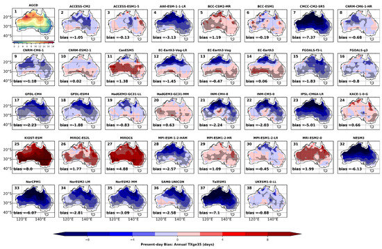
Figure 7.
Climatological mean annual bias in the number of days when maximum temperature is greater than 35 C (Txge35: days) relative to the Australian Gridded Climate Data dataset (AGCD; panel 1) for the individual CMIP6 GCMs (panels 2–38). Data spans 1951–2014. Stippling indicates statistically significant differences using a student’s t-test at the 95% confidence level.
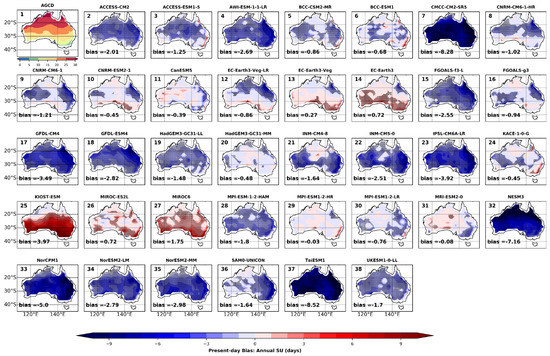
Figure 8.
Climatological mean annual bias in summer days (number of days when maximum temperature > 25 °C) (SU: days) relative to the Australian Gridded Climate Data dataset (AGCD; panel 1) for the individual CMIP6 GCMs (panels 2–38). Data spans 1951–2014. Stippling indicates statistically significant differences using a student’s t-test at the 95% confidence level.
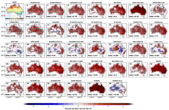
Figure 9.
Climatological mean annual bias in the minimum minimum temperature (TNn: °C) relative to the Australian Gridded Climate Data dataset (AGCD; panel 1) for the individual CMIP6 GCMs (panels 2–38). Data spans 1951–2014. Stippling indicates statistically significant differences using a student’s t-test at the 95% confidence level.
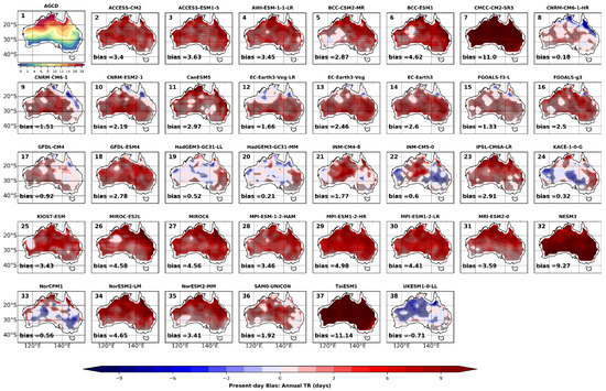
Figure 10.
Climatological mean annual bias in tropical nights (number of days when minimum temperature > 20 °C (TR: days) relative to Australian Gridded Climate Data dataset (AGCD; panel 1), for the individual CMIP6 GCMs (panels 2–38). Data spans 1951–2014. Stippling indicates statistically significant differences using a student’s t-test at the 95% confidence level.
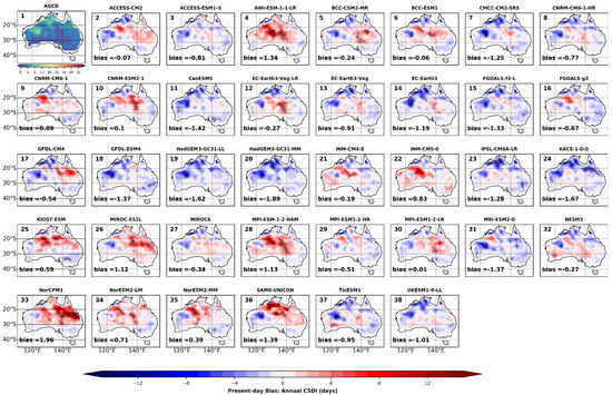
Figure 11.
Climatological mean annual bias in the annual count of nights with at least 4 consecutive nights when daily minimum temperature < 10th percentile (CSDI: days) relative to Australian Gridded Climate Data dataset (AGCD; panel 1), for the individual CMIP6 GCMs (panels 2–38). Data spans 1951–2014. Stippling indicates statistically significant differences using a student’s t-test at the 95% confidence level.
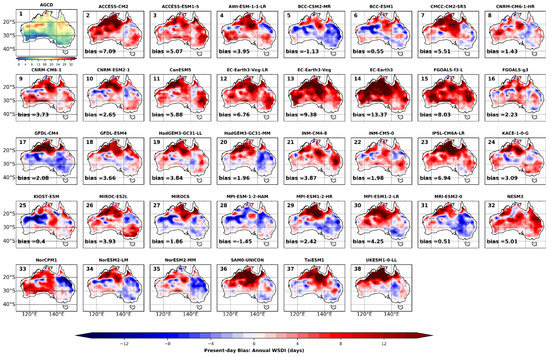
Figure 12.
Climatological mean annual bias in the annual count of days with at least 4 consecutive days when daily maximum temperature > 90th percentile (WSDI: days) relative to Australian Gridded Climate Data dataset (AGCD; panel 1), for the individual CMIP6 GCMs (panels 2–38). Data spans 1951–2014. Stippling indicates statistically significant differences using a student’s t-test at the 95% confidence level.
In Figure 6, GCMs KIOST-ESM, MIR°C6, CanESM5 and MRI-ESM2-0 show the strongest warm biases (~ 2–8 °C), whereas NorCPM1, NorESM2-LM and NorESM2-MM (Norwegian Climate Centre), TaiESM1, IPSL-CM6A-LR and CMCC-CM2-SR5 show the strongest cold bias (~ −2 to −10 °C) throughout the continent. Previously, Alexander & Arblaster (2017) [11] evaluated CMIP5 GCMs and noted that GCMs from the MIR°C family show a strong warm bias over Australia. Our results are broadly consistent with these findings. Most GCMs typically show cold bias ranging from −1 to −3 °C. Txge35 (Figure 7) and SU (Figure 8) follow a similar pattern to TXx, and the GCMs with warm bias in TXx also overestimate TXge35 and SU, whereas GCMs with cold bias in TXx, underestimate TXge35 and SU.
Overall, for hot extremes (TXx, Txge35 and SU), BCC-ESM1, CNRM-ESM2-1, EC-Earth3-Veg, EC-Earth3, HadGEM3-GC31-MM, MPI-ESM1-2-HR and KACE-1-0-G are found to be top-performing GCMs whereas CMCC-CM2-SR5, IPSL-CM6A-LR, KIOST-ESM, MIR°C6, NESM3, NorCPM1, NorESM2-MM and TaiESM1 are found to be the worst-performing GCMs (Table 3).
For TNn (Figure 9), most GCMs typically show warm biases over the entire continent. The GCMs GFDL-CM4 and UKESM1-0-LL show slight cold biases in western and eastern Australia. However, the magnitude of these biases is small (~ −0.2–0.5 °C). CanESM5, GFDL-CM4, KACE-1-0-G, UKESM1-0-LL, HadGEM3-GC31-LL, HadGEM3-GC31-MM (Hadley Centre), INM-CM4-8 and INM-CM5-0 (INM Russia) show the smallest bias. TaiESM1, CMCC-CM2-SR5 and NESM3 show the largest bias of ~ −7 to −8.5 °C (Table 3). The GCMs with large warm biases in TNn (TaiESM1, CMCC-CM2-SR5 and NESM3) also show large overestimations in TR (Figure 10 ~10–12 days). For all other GCMs, overestimation in TR varies between 2–5 days.
The GCMs typically overestimate CSDI in northern and central Australia, whereas they underestimate cold spell durations over other parts of Australia, including the heavily populated east coast (Figure 11). However, these biases are not found to be significant. GFDL-ESM4, HadGEM3-1LL, HadGEM3-GC31-MM and KACE-1-0G show underestimation throughout the domain. In terms of bias magnitude, ACCESS-CM2, BCC-CSM2-MR and BCC-ESM1 (Beijing Climate Centre), CNRM-CM6-1, CNRM-ESM2-1, EC-Earth3-Veg-LR, INM-CM4-8, MPI-ESM1-2-LR and NESM3 show the smallest bias (<0.3 days), whereas NorCPM1, SAMO-UNICON, CanESM5, GFDL-ESM4, HadGEM3-GC31-LL and HadGEM3-GC31-MM (Hadley Centre), MRI-ESM2-0 and AWI-ESM-1-1LR show the largest biases (>1 day).
For WSDI (Figure 12), biases are much larger than CSDI. The large biases in WSDI compared to CSDI can be attributed to the observed WSDI (Figure 12, panel 1) typically being 4-times higher than CDSI (Figure 11, panel 1). Here, except for ACCESS-CM2 and ACCESS-ESM1-5 (Australian Community) and EC-Earth-Veg-LR, EC-Earth3-Veg and EC-Earth3 (EC-Earth consortium), all other GCMs overestimate warm spells in northern and central Australia and underestimate them in other parts of the domain. Positive biases are mostly significant, whereas negative biases are mostly not significant. The EC-Earth consortium GCMs show the largest bias (~ >8 days), followed by ACCESS-CM2, CanESM5, FGOALS-f3-L, IPSL-CM6A-LR, TaiESM1 and UKESM1-0-LL.
Similar to precipitation extremes, the biases at the seasonal scale for temperature extremes (TXx (Figures S17–S20), Txge35 (Figure S21–S24), SU (Figures S25–S28), TNn (Figures S29–S32) and TR (Figures S33–S36) mimicked the annual biasesz (Supplementary Materials), i.e., GCMs with cold and warm biases at annual scales also exhibit cold and warm seasonal biases, respectively, and these biases have approximately similar spatial distributions. For impact modellers and stakeholders using GCM data, bias corrections of extremes are recommended.
In terms of RMSE, for all the temperature extremes except WSDI and CSDI, a common pattern is seen, i.e., GCMs that show large biases also show large RMSEs and vice versa (Table 4). Hence, the evaluation of GCM performance remains robust across bias and RMSE for all temperature extremes except WSDI and CSDI. For WSDI, there seems to be some overlap in the best and worst performing GCMs as measured by bias and RMSE, with a few exceptions such as AWI-ESM-1-1-LR and TaiESM1 (which show large RMSEs and small bias). For CSDI, there is more variance in results, and the biases are found to be mostly not significant. Due to this, GCMs which are the worst performers for bias (GFDL-ESM4, HadGEM3-GC31-LL, HadGEM3-GC31-MM, CanESM5 and KACE-1-0-G) are found to be among the best performers for RMSE.
For PCorr (Table 5), the GCM performance ranking does not completely align with that of other metrics (bias, RMSE and IVS). For example, MPI-ESM-1-2-HAM, MPI-ESM-1-2-LR and MPI-ESM-1-2-HR (MPI Germany) and MRI-ESM2-0 are among the best performers for PCorr for more than three extremes. However, these GCMs are not in the best performing subset for other metrics (bias, RMSE and IVS). For IVS, GCMs show overlap in the best and worst performing subset for most of the extremes; for example, INM-CM4-8, INM-CM5-0, IPSL-CM6A-LR, KACE-1-0-G and CNRM-ESM2-1 are found to be the best performers whereas AWI-ESM-1-1-LR, CMCC-CM2-SR5, KIOST-ESM, MIR°C6, MPI-ESM1-2-LR are found to be the worst performers for more than three extremes. The GCMs ranking for IVS is thus roughly comparable with bias and RMSE.
3.2. Normalisation and Averaging
We calculate the continental means of biases and RMSEs, then normalise (based on Equations (3) and (4)) and average all the metrics (bias, RMSE, PCorr, IVS) for all indices. For the extreme indices available at the monthly timescale (Table 2), 20 normalised metrics (i.e., bias, RMSE, PCorr and IVS for Annual, DJF, MAM, JJA and SON, respectively) are calculated (Figure 13). In contrast, for the extreme indices only available at the annual timescale (Table 2), four normalised metrics (i.e., bias, RMSE, PCorr and IVS for Annual) are generated (Figure 14).
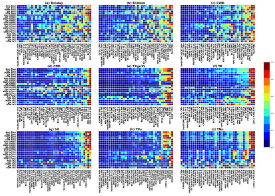
Figure 13.
Normalised and continentally averaged annual and seasonal means of individual metrics (bias, root mean square error (RMSE), pattern correlation (PCorr) and interannual variability score (IVS)) for the extreme indices (a) maximum 1-day precipitation (Rx1Day), (b) number of very heavy rain days (rain > 10 mm) (R10mm), (c) consecutive wet days (CWD), (d) consecutive dry days (CDD), (e) number of days when maximum temperature is greater than 35 °C (Txge35), (f) tropical nights (number of days when minimum temperature > 20 °C) (TR), (g) summer days (number of days when maximum temperature > 25 °C) (SU), (h) maximum maximum-temperature (TXx) and (i) minimum minimum-temperature (TNn). Here, the smaller values of normalised metrics correspond to the better performance of GCMs. Moreover, for each extreme index, GCMs are arranged from best to worst performance as we move from left and right. Data spans 1951–2014.
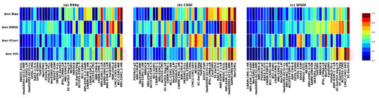
Figure 14.
Normalised and continentally averaged annual means of individual metrics (bias, root mean square error (RMSE), pattern correlation (PCorr) and interannual variability score (IVS)) for the extreme indices (a) total annual precipitation from very heavy rain days (R99p), (b) annual count of nights with at least 4 consecutive nights when daily minimum temperature < 10th percentile (CSDI) and (c) annual count of days with at least 4 consecutive days when daily maximum temperature > 90th percentile (WSDI). Here, the smaller values of normalised metrics correspond to the better performance of GCMs. Moreover, for each extreme index, GCMs are arranged from best to worst performance as we move from left and right. Data spans 1951–2014.
Overall, for both precipitation and temperature extremes (Figure 13 and Figure 14), we find that the top performing GCMs consistently score well (<0.2) in most metrics, capturing the magnitude, spatial and temporal patterns of the observed field. In contrast, the poorly performing GCMs are less skilled at capturing spatial and temporal patterns. For temperature extremes (except for CSDI and WSDI), approximately 5–7 GCMs perform poorly (normalised mean score of all metrics > 0.6) (Figure 13e–i). For precipitation extremes, 15–17 GCMs perform poorly (normalised score > 0.6) at capturing the spatial and temporal pattern of the observed field (Figure 13a–d). These results suggest that GCMs show higher overall skill in capturing observed temperature extremes. In contrast, many GCMs struggle to replicate observed precipitation extremes, with only a small subset of high-skill GCMs. These results reflect the findings of previous studies [11,21,22], which have suggested that GCMs struggle to capture precipitation and its extremes.
Based on these results, we find that HadGEM3-GC31-MM, HadGEM3-GC31-LL (Hadley Centre), GFDL-CM4, GFDL-ESM4 (NOAA), UKESM1-0-LL, KACE-1-0-G, and MRI-ESM2-0 tend to show consistently good performance for more than 50% of the extreme precipitation indices analysed in this study. Whereas GCMs INM-CM4-8, INM-CM5-0 (INM Russia), MPI-ESM1-2-LR, MPI-ESM1-2-HR (MPI Germany), MIR°C6, NorCPM1, BCC-ESM1 and IPSL-CM6A-LR tend to show consistently poor performance for more than 50% of the extreme precipitation indices.
For Australian temperature extremes, consistently good performing GCMs for more than 50% of the extreme indices are: BCC-ESM1, HadGEM3-GC31-MM, CNRM-CM6-1-HR, CNRM-ESM2-1, FGOALS-g3, MPI-ESM1-2-LR, GFDL-ESM4 and GFDL-CM4 (NOAA), and KACE-1-0G whereas the consistently poor performing GCMs are: KIOST-ES, MIR°C6, CMCC-CM2-SR5, TaiESM1, MIR°C-ES2L, NorCPM1, and NESM3.
Considering both precipitation and temperature extremes, HadGEM3-GC31-MM, HadGEM3-GC31-LL (Hadley Centre), UKESM1-0-LL, FGOALS-g3, GFDL-ESM4 and GFDL-CM4 (NOAA) show consistently good performance. Conversely, CMCC-CM2-SR5, MIR°C6, NESM3 and NorCPM1 consistently perform poorly in replicating Australian temperature and precipitation extremes.
We also compare the overall GCM performance ranking at the continental scale with performance calculated for the four Natural Resource Management (NRM) regions (Figure S37) to assess if GCM performance varies for different regions (Figure 15). The four NRM regions are named southern Australia (south), eastern Australia (east), northern Australia (north), and Rangelands covering the central area (centre). These regions are broadly aligned with climatological boundaries (CSIRO and Bureau of Meteorology 2015 [65]; Fiddes et al. 2021 [66]) and align with the IPCC reference regions [67]. Examining the performance of GCMs over these regions is particularly important when considering the design of regional downscaling experiments or assessing regional scale climate impacts. For example, regional climate projections like New South Wales (NSW) and Australian Regional Climate Modelling (NARCliM) are made by choosing a subset of best-performing GCMs over a smaller sub-domain which falls within eastern and southern Australia NRM regions [68,69]. This analysis will be of strong interest for producing updated national climate change projections for Australia and providing new insights into the climate system and climate change relevant to the region.
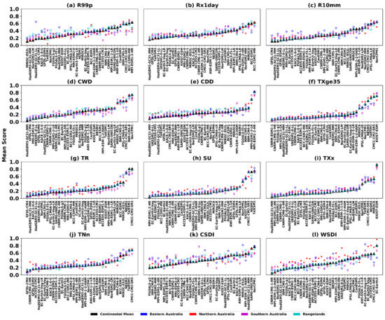
Figure 15.
Spatially averaged normalised scores of the GCMs for the extreme indices (a) total annual precipitation from very heavy rain days (R99p), (b) maximum 1-day precipitation (Rx1Day), (c) number of very heavy rain days (rain > 10 mm) (R10mm), (d) consecutive wet days (CWD), (e) consecutive dry days (CDD), (f) number of days when maximum temperature is greater than 35 °C (Txge35), (g) tropical nights (number of days when minimum temperature > 20 °C) (TR), (h) summer days (number of days when maximum temperature > 25 °C) (SU), (i) maximum maximum-temperature (TXx), (j) minimum minimum-temperature (TNn), (k) annual count of nights with at least 4 consecutive nights when daily minimum temperature < 10th percentile (CSDI) and (l) annual count of days with at least 4 consecutive days when daily maximum temperature > 90th percentile (WSDI). Here, the smaller score values correspond to the better performance of GCMs. Also, for each extreme index, GCMs are arranged from best to worst performance as we move from left and right. Here black, blue, red, magenta and cyan colours denote means over the continent, eastern Australia, northern Australia, southern Australia and rangelands. The markers denote the continental (triangle), northern Australia (star), eastern Australia (circle), southern Australia (diamond) and rangelands (square) values. Data spans 1951–2014.
The result reveals that for all the extreme precipitation indices (except R99p), GCM performance does not show much regional variance and performance rankings remain the same for the continent and the four sub-regions (Figure S37). In contrast, for R99p (Figure 15a), some GCMs show notable inter-regional differences. For example, HadGEM3-GC31-LL is one of the worst performers in eastern Australia whereas it is among the best for continental scale and other regions. A similar pattern is also seen for ACCESS-CM2. This GCM is one of the best performers for southern Australia; however, it remains in the mid-range performance on a continental scale and for other regions.
For all the temperature extremes except WSDI and CSDI (Figure 15k,l), GCM performance at the continental and regional scale show little variance. However, for WSDI and CSDI, strong inter-regional differences are observed for eastern, northern, and southern Australia.
Previous studies have also shown that for different climate variables, GCM performance varies in different regions [70,71]. This is related to how GCMs represent the land cover, terrain morphology, and climate zones which are crucial for the simulation of particular climate variables.
4. Discussion and Conclusions
Di Virgilio et al. 2022 [33] evaluated CMIP6 GCMs for downscaling over Australia by assessing individual GCMs against criteria like performance simulating daily climate variable distributions, climate means, extremes, and modes; model independence; and climate change signal diversity. Grose et al. 2020 [32] evaluated how the CMIP6 ensemble performs in comparison to CMIP5 for present and future climates. A recent study by Zhang et al. 2022 [72] evaluated the performance of CMIP6 GCMs over the Australia CORDEX domain by examining the climatological mean and interannual variability. However, none of these studies comprehensively examined the climate extremes in Australia. We, in this study, present the detailed evaluation of 12 extreme precipitation and temperature indices as simulated by 37 CMIP6 GCMs. Although this study did not evaluate all possible aspects of GCM performance, it aimed to select some key evaluation metrics fundamental to characterising GCM performance for simulating climate extremes.
Our results show that overall, CMIP6 GCMs underestimate precipitation intensity and overestimate wet days, overestimate minimum temperature extremes, and underestimate maximum temperature extremes. We also find that a greater number of GCMs show high skill in capturing the observed temperature extremes, whereas GCMs typically show low skill for precipitation extremes. Past studies have suggested that GCMs typically struggle to capture the observed changes in precipitation extremes due to multiple factors [73]. For example, the inability of GCMs to simulate internal variability in heavy regional precipitation, statistical effects of different grid resolutions of GCMs and observations, and the inability to resolve convective processes due to convective parametrisations used by the GCMs [74].
We find a subset of GCMs (HadGEM3-GC31-MM and HadGEM3-GC31-LL (Hadley Centre), UKESM1-0-LL, FGOALS-g3, and GFDL-ESM4 and GFDL-CM4 (NOAA)) that tend to show consistently good performance for more than 50% of climate extremes analysed in this study and across a broad suite of evaluation metrics. Our results are comparable to the recent study by Srivastava et al. (2020) [43] and Ayugi et al. (2021) [26], who evaluated the performance of CMIP6 GCMs for simulating precipitation extremes over the United States and East Africa, respectively. Both studies showed that HadGEM3-GC31-LL and UKESM1-0-LL consistently show good performance for the United States and East Africa.
We also find that a subset of GCMs (CMCC-CM2-SR5, MIR°C6, NESM3 and NorCPM1) tend to perform poorly overall. It is well known that some aspects of climate are poorly represented in all GCMs due to common limitations in model parametrisations and spatial resolution. For example, Chen et al. (2021) [45] showed that the convective parametrisation in most CMIP5 GCMs typically leads to a slight drizzling bias. In contrast, Alexander and Arblaster (2017) [11] showed that CMIP5 GCMs tend to slightly overestimate minimum temperature extremes and underestimate maximum temperature extremes. However, we find that the poor performing GCMs tend to show unrealistic errors compared to common errors found in most GCMs. For example, CMCC-CM2-SR5, MIR°C6, NESM3 and NorCPM1 were found to perform extremely poorly for most of the extreme indices analysed in this study. The magnitude of biases shown in these GCMs was exceptionally high compared to the median bias across the 37 GCMs. Past study has shown that GCMs showing unrealistic errors are often those for which projections lie on the margins of or outside the range of most of the ensemble [75].
The paper’s results also highlighted that resolution does not appear to be a deciding factor in how well a model performs at reproducing temperature/precipitation indices for Australia. For example, the relatively high-resolution CNRM-CM6-1 does not necessarily ‘outperform’ lower resolution models such as BCC-ESM1. The key factor that is more closely tied to the model performance is the ‘model family’. GCMs from the same parent institution and GCMs from different institutions that share key model components either do a good or bad job in capturing the broad-scale features and processes of the climate, resulting in similar model performance. For example, in GCMs from the same parent institution (GCMs from MPI Germany, INM Russia, Beijing Climate Centre etc.), if one model version is too hot or too wet, then this is apparent in all the model versions. GCMs from the Australian community, UK Met Office Hadley Centre, NOAA-GFDL and UKESM1-0-LL, which share atmospheric model codes, also indicate similar results. Past studies have also reported a similar impact of the ‘model family’ on the GCM performance of CMIP3 [10] and CMIP5 models [11]. The large dependence of different versions of models on the model ‘family’ highlights an important issue regarding model dependence and whether we are using false assumptions that these multiple simulations all constitute independent samples (e.g., Abramowitz 2010 [76]; Abramowitz and Bishop 2015 [77]).
Although this study provides a comprehensive evaluation of CMIP6 GCMs, it also has some caveats. This study assessed the performance of CMIP6 GCMs in simulating climate extremes using a metric-based approach. It should be recognised that models are complex in nature, and summarising the performance of models using a few metrics is quite challenging and may be inadequate. In addition to the limitations in performance metrics, the choice of reference dataset also affects the performance of models. Past studies have shown that the reference dataset’s choice can bias the model performance results [22,78,79].
In this study, we used the Rupp et al. (2013) [54] normalisation method, which normalised the GCMs based on the maximum and minimum value of the metric among the GCMs. Normalisation is performed such that different metrics can be fairly compared. This method assumes the spread of each metric for all the GCMs is relatively equal. This assumption is not necessarily true; thus, this method can bias the results, as it is possible to subdivide the GCMs and manipulate rankings by changing the relative weights between the different metrics. For example, if a single GCM performs extraordinarily poorly in only one metric, the inclusion of that GCM greatly reduces the importance of that metric as the normalisation factor becomes too small because of the range being extremely large.
Despite these limitations, our study has important implications for multiple systems affected by climate extremes. For instance, our evaluation shows that precipitation extremes typically record the largest bias in Australia’s northern and eastern parts. The northern part of Australia is the region belonging to the northern monsoon cluster. This region receives widespread rainfall from the large oceanic mesoscale convective systems [80]. Past studies have shown that GCMs typically struggle to simulate the characteristic of mesoscale convective systems with reasonable accuracy and thus record large errors in monsoon-dominated regions [70,81,82,83,84]. The eastern part of Australia is a region of complex topography composed of mountains, alpines, and lakes [85]. Past studies have shown that the topography of GCMs is generally smoother and lower in elevation than that in reality [86]. For this reason, GCMs typically record large biases over these regions [87]. Northern Australia is a major region for agricultural production, whereas eastern coastlines are where more than 50% of the Australian population resides. The large uncertainty in GCM performances over these economically and societally important regions reveals the limitations of GCMs for their application in studying impacts from precipitation and temperature extremes over these areas.
The results of this study are useful for identifying potential CMIP6 GCMs for performing exercises like dynamical downscaling experiments as part of endeavours such as CORDEX Australasia. Regional climate modelling helps provide information at fine, sub-GCM grid scales, which is more suitable for studies of regional phenomena and application to vulnerability, climate impacts, and adaptation assessments. However, we acknowledge that for selecting potential GCMs for dynamical downscaling, additional and more comprehensive evaluations like the GCM performance for simulating mean climate, and climate drivers like El Niño, Southern Annular mode, etc., should be undertaken to rank the overall GCM performance. An in-depth analysis of physical processes is also required to identify the cause of the model bias. Another crucial factor is selecting GCMs based on the sign of GCM future climate change signals.
Modelling factors like choice of model physics and land-atmosphere coupling in the GCMs can directly affect precipitation and temperature extremes. Analysing and attributing the GCMs with respect to these factors was beyond the scope of this study. However, it will be crucial to investigate further to identify what modelling factors contribute to the high and poor skill in GCMs for simulating different extreme indices.
Supplementary Materials
The following supporting information can be downloaded at: https://www.mdpi.com/article/10.3390/atmos13091478/s1, Figure S1. Climatological mean December-January-February bias in maximum 1-day precipita-tion (Rx1Day: mm) relative to Australian Gridded Climate Data dataset (AGCD; panel 1), for the individual CMIP6 GCMs (panels 2–38). Data spans 1951–2014. Stippling indicates statistically significant differences using a student’s t-test at the 95% confidence level. The white mask in part of the inland domain are the regions with no station data. Figure S2. Same as S1 but for March-April-May. Figure S3. Same as S1 but for June-July-August. Figure S4. Same as S1 but for September-October-November. Figure S5. Climatological mean December-January-February bias in number of very heavy rain days (rain > 10 mm) (R10mm: days) relative to Australian Gridded Climate Data dataset (AGCD; panel 1), for the individual CMIP6 GCMs (panels 2–38). Data spans 1951–2014. Stippling indicates statistically significant differences using a student’s t-test at the 95% confidence level. The white mask in part of the inland domain are the regions with no station data. Figure S6. Same as S5 but for March-April-May. Figure S7. Same as S5 but for June-July-August. Figure S8. Same as S5 but for September-October-November. Figure S9. Climatological mean December-January-February bias in consecutive wet days (CWD: days) relative to Australian Gridded Climate Data dataset (AGCD; panel 1), for the indi-vidual CMIP6 GCMs (panels 2–38). Data spans 1951–2014. Stippling indicates statistically signif-icant differences using a student’s t-test at the 95% confidence level. The white mask in part of the inland domain are the regions with no station data. Figure S10. Same as S9 but for March-April-May. Figure S11. Same as S9 but for June-July-August. Figure S12. Same as S9 but for September-October-November. Figure S13. Climatological mean December-January-February bias in consecutive dry days (CDD: days) relative to Australian Gridded Climate Data dataset (AGCD; panel 1), for the in-dividual CMIP6 GCMs (panels 2–38). Data spans 1951–2014. Stippling indicates statistically sig-nificant differences using a student’s t-test at the 95% confidence level. The white mask in part of the inland domain are the regions with no station data. Figure S14. Same as S13 but for March-April-May. Figure S15. Same as S13 but for June-July-August. Figure S16. Same as S13 but for September-October-November. Figure S17. Climatological mean December-January-February bias in maximum maxi-mum-temperature (TXx: oC) relative to Australian Gridded Climate Data dataset (AGCD; panel 1), for the individual CMIP6 GCMs (panels 2–38). Data spans 1951–2014. Stippling indicates sta-tistically significant differences using a student’s t-test at the 95% confidence level. The white mask in part of the inland domain are the regions with no station data. Figure S18. Same as S17 but for March-April-May. Figure S19. Same as S17 but for June-July-August. Figure S20. Same as S17 but for September-October-November. Figure S21. Climatological mean December-January-February bias in number of days when maximum temperature is greater than 35 C (Txge35: days) relative to Australian Gridded Cli-mate Data dataset (AGCD; panel 1), for the individual CMIP6 GCMs (panels 2–38). Data spans 1951–2014. Stippling indicates statistically significant differences using a student’s t-test at the 95% confidence level. The white mask in part of the inland domain are the regions with no sta-tion data. Figure S22. Same as S21 but for March-April-May. Figure S23. Same as S21 but for June-July-August. Figure S24. Same as S21 but for September-October-November. Figure S25. Climatological mean December-January-February bias in summer days (number of days when maximum temperature > 25 °C) (SU: days) relative to Australian Gridded Climate Data dataset (AGCD; panel 1), for the individual CMIP6 GCMs (panels 2–38). Data spans 1951–2014. Stippling indicates statistically significant differences using a student’s t-test at the 95% confidence level. The white mask in part of the inland domain are the regions with no station data. Figure S26. Same as S25 but for March-April-May. Figure S27. Same as S25 but for June-July-August. Figure S28. Same as S25 but for September-October-November. Figure S29. Climatological mean December-January-February bias in minimum mini-mum-temperature (TNn: oC) relative to Australian Gridded Climate Data dataset (AGCD; panel 1), for the individual CMIP6 GCMs (panels 2–38). Data spans 1951–2014. Stippling indicates sta-tistically significant differences using a student’s t-test at the 95% confidence level. The white mask in part of the inland domain are the regions with no station data. Figure S30. Same as S29 but for March-April-May. Figure S31. Same as S29 but for June-July-August. Figure S32. Same as S29 but for September-October-November. Figure S33. Climatological mean December-January-February bias in tropical nights (number of days when minimum temperature > 20 °C (TR: days) relative to Australian Gridded Climate Data dataset (AGCD; panel 1), for the individual CMIP6 GCMs (panels 2–38). Data spans 1951–2014. Stippling indicates statistically significant differences using a student’s t-test at the 95% confi-dence level. The white mask in part of the inland domain are the regions with no station data. Figure S34. Same as S33 but for March-April-May. Figure S35. Same as S33 but for June-July-August. Figure S36. Same as S33 but for September-October-November. Figure S37. (Figure 3 from Grose et al. 2020). Here red lines indicate the borders of the four “supercluster” averaging regions: Northern Australia (North), Rangelands (Centre), Southern Australia (South), Eastern Australia (East). Given that there is a substantial distinction between the coastal (temperate) East, versus the semi-arid inland East.
Author Contributions
N.N. conducted all the analyses and led the writing of the paper. G.D.V., F.J., E.T., K.B. and M.L.R. assisted in the interpretation and writing of the paper. All authors have read and agreed to the published version of the manuscript.
Funding
This research was funded by NSW Climate Change Fund.
Institutional Review Board Statement
Not applicable.
Informed Consent Statement
Not applicable.
Data Availability Statement
CMIP6 data supporting this study’s findings are freely available from ESGF (https://esgf-node.llnl.gov/search/cmip6/, accessed on 1 November 2020). Details about AGCD are available at the Australian Bureau of Meteorology website (http://www.bom.gov.au/metadata/catalogue/19115/ANZCW0503900567, accessed on 1 November 2020). The dataset is available on the NCI (National Computational Infrastructure) server in project zv2. Detail on how to access the data can be found at http://climate-cms.wikis.unsw.edu.au/AGCD (accessed on 1 November 2020).
Acknowledgments
This work is made possible by funding from the NSW Climate Change Fund for NSW and the Australian Regional Climate Modelling (NARCliM) Project. We thank the climate modelling groups for producing and making available their model outputs, the Earth System Grid Federation (ESGF) for archiving the data and providing access, and the multiple funding agencies who support CMIP3, CMIP5 and the Earth System Grid Federation (ESGF).
Conflicts of Interest
The authors declare no conflict of interest.
References
- Masson-Delmotte, V.; Zhai, P.; Pirani, A.; Connors, S.L.; Péan, C.; Berger, S.; Zhou, B. Climate Change 2021: The Physical Science Basis. Contribution of Working Group I to the Sixth Assessment Report of the Intergovernmental Panel on Climate Change, 2. 2021. Available online: https://www.ipcc.ch/report/ar6/wg1/ (accessed on 1 November 2021).
- Kiem, A.S.; Johnson, F.; Westra, S.; van Dijk, A.; Evans, J.P.; O’Donnell, A.; Mehrotra, R. Natural hazards in Australia: Droughts. Clim. Chang. 2016, 139, 37–54. [Google Scholar] [CrossRef]
- Walsh, K.; White, C.J.; McInnes, K.; Holmes, J.; Schuster, S.; Richter, H.; Warren, R.A. Natural hazards in Australia: Storms, wind and hail. Clim. Chang. 2016, 139, 55–67. [Google Scholar] [CrossRef]
- Johnson, F.; Hutchinson, M.F.; The, C.; Beesley, C.; Green, J. Topographic relationships for design rainfalls over Australia. J. Hydrol. 2016, 533, 439–451. [Google Scholar] [CrossRef]
- Perkins-Kirkpatrick, S.E.; White, C.J.; Alexander, L.V.; Argüeso, D.; Boschat, G.; Cowan, T.; Purich, A. Natural hazards in Australia: Heatwaves. Clim. Chang. 2016, 139, 101–114. [Google Scholar] [CrossRef]
- Zander, K.K.; Botzen, W.J.; Oppermann, E.; Kjellstrom, T.; Garnett, S.T. Heat stress causes substantial labour productivity loss in Australia. Nat. Clim. Chang. 2015, 5, 647–651. [Google Scholar] [CrossRef]
- Westra, S.; White, C.J.; Kiem, A.S. Introduction to the special issue: Historical and projected climatic changes to Australian natural hazards. Clim. Chang. 2016, 139, 1–26. [Google Scholar] [CrossRef]
- Plummer, N.; Salinger, M.J.; Nicholls, N.; Suppiah, R.; Hennessy, K.J.; Leighton, R.M.; Lough, J.M. Changes in climate extremes over the Australian region and New Zealand during the twentieth century. Weather. Clim. Extrem. 1999, 42, 183–202. [Google Scholar]
- Haylock, M.; Nicholls, N. Trends in extreme rainfall indices for an updated high-quality data set for Australia, 1910–1998. Int. J. Climatol. A J. R. Meteorol. Soc. 2000, 20, 1533–1541. [Google Scholar] [CrossRef]
- Alexander, L.V.; Arblaster, J.M. Assessing trends in observed and modelled climate extremes over Australia in relation to future projections. Int. J. Climatol. A J. R. Meteorol. Soc. 2009, 29, 417–435. [Google Scholar] [CrossRef]
- Alexander, L.V.; Arblaster, J.M. Historical and projected trends in temperature and precipitation extremes in Australia in observations and CMIP5. Weather Clim. Extrem. 2017, 15, 34–56. [Google Scholar] [CrossRef]
- Min, S.K.; Cai, W.; Whetton, P. Influence of climate variability on seasonal extremes over Australia. J. Geophys. Res. Atmos. 2013, 118, 643–654. [Google Scholar] [CrossRef]
- Nishant, N.; Sherwood, S.C. How strongly are mean and extreme precipitation coupled? Geophys. Res. Lett. 2021, 48, e2020GL092075. [Google Scholar] [CrossRef]
- Herold, N.; Ekström, M.; Kala, J.; Goldie, J.; Evans, J.P. Australian climate extremes in the 21st century according to a regional climate model ensemble: Implications for health and agriculture. Weather Clim. Extrem. 2018, 20, 54–68. [Google Scholar] [CrossRef]
- King, A.D.; Karoly, D.J.; Henley, B.J. Australian climate extremes at 1.5 C and 2 C of global warming. Nat. Clim. Chang. 2017, 7, 412–416. [Google Scholar] [CrossRef]
- King, A.D.; Black, M.T.; Min, S.K.; Fischer, E.M.; Mitchell, D.M.; Harrington, L.J.; Perkins-Kirkpatrick, S.E. Emergence of heat extremes attributable to anthropogenic influences. Geophys. Res. Lett. 2016, 43, 3438–3443. [Google Scholar] [CrossRef]
- Bradstock, R.A.; Hammill, K.A.; Collins, L.; Price, O. Effects of weather, fuel and terrain on fire severity in topographically diverse landscapes of south-eastern Australia. Landsc. Ecol. 2010, 25, 607–619. [Google Scholar] [CrossRef]
- Zheng, B.; Chenu, K.; Fernanda Dreccer, M.; Chapman, S.C. Breeding for the future: What are the potential impacts of future frost and heat events on sowing and flowering time requirements for Australian bread wheat (Triticum aestivium) varieties? Glob. Chang. Biol. 2012, 18, 2899–2914. [Google Scholar] [CrossRef]
- Yilmaz, A.G.; Hossain, I.; Perera, B.J.C. Effect of climate change and variability on extreme rainfall intensity–frequency–duration relationships: A case study of Melbourne. Hydrol. Earth Syst. Sci. 2014, 18, 4065–4076. [Google Scholar] [CrossRef]
- Nairn, J.R.; Fawcett, R.J. The excess heat factor: A metric for heatwave intensity and its use in classifying heatwave severity. Int. J. Environ. Res. Public Health 2015, 12, 227–253. [Google Scholar] [CrossRef]
- Seneviratne, S.; Nicholls, N.; Easterling, D.; Goodess, C.; Kanae, S.; Kossin, J.; Zwiers, F.W. Changes in climate extremes and their impacts on the natural physical environment. In Managing the Risks of Extreme Events and Disasters to Advance Climate Change Adaptation; A Special Report of Working Groups I and II of the Intergovernmental Panel on Climate Change (IPCC); Field, C.B., Barros, V.T.F., Stocker, D., Qin, D.J., Dokken, K.L., Ebi, M.D., Mastrandrea, K.J., Mach, G.-K., Plattner, S.K., Allen, M., et al., Eds.; Cambridge University Press: Cambridge, UK; New York, NY, USA, 2012; pp. 109–230. [Google Scholar]
- Sillmann, J.; Kharin, V.V.; Zhang, X.; Zwiers, F.W.; Bronaugh, D. Climate extremes indices in the CMIP5 multimodel ensemble: Part 1. Model evaluation in the present climate. J. Geophys. Res. Atmos. 2013, 118, 1716–1733. [Google Scholar] [CrossRef]
- Ongoma, V.; Chen, H.; Gao, C.; Nyongesa, A.M.; Polong, F. Future changes in climate extremes over Equatorial East Africa based on CMIP5 multimodel ensemble. Nat. Hazards 2018, 90, 901–920. [Google Scholar] [CrossRef]
- Xu, K.; Wu, C.; Hu, B.X. Projected changes of temperature extremes over nine major basins in China based on the CMIP5 multimodel ensembles. Stoch. Environ. Res. Risk Assess. 2019, 33, 321–339. [Google Scholar] [CrossRef]
- Wu, C.; Yeh, P.J.F.; Chen, Y.Y.; Hu, B.X.; Huang, G. Future precipitation-driven meteorological drought changes in the CMIP5 multimodel ensembles under 1.5 °C and 2 °C global warming. J. Hydrometeorol. 2020, 21, 2177–2196. [Google Scholar] [CrossRef]
- Ayugi, B.; Jiang, Z.; Zhu, H.; Ngoma, H.; Babaousmail, H.; Karim, R.; Dike, V. Comparison of CMIP6 and CMIP5 models in simulating mean and extreme precipitation over East Africa. Int. J. Climatol. 2021, 41, 6474–6496. [Google Scholar] [CrossRef]
- Jiang, Z.; Li, W.; Xu, J.; Li, L. Extreme precipitation indices over China in CMIP5 models. Part I: Model evaluation. J. Clim. 2015, 28, 8603–8619. [Google Scholar] [CrossRef]
- Kumar, D.; Mishra, V.; Ganguly, A.R. Evaluating wind extremes in CMIP5 climate models. Clim. Dyn. 2015, 45, 441–453. [Google Scholar] [CrossRef]
- Eyring, V.; Bony, S.; Meehl, G.A.; Senior, C.A.; Stevens, B.; Stouffer, R.J.; Taylor, K.E. Overview of the Coupled Model Intercomparison Project Phase 6 (CMIP6) experimental design and organization. Geosci. Model Dev. 2016, 9, 1937–1958. [Google Scholar] [CrossRef]
- Taylor, K.E.; Stouffer, R.J.; Meehl, G.A. An overview of CMIP5 and the experiment design. Bull. Am. Meteorol. Soc. 2012, 93, 485–498. [Google Scholar] [CrossRef]
- Stouffer, R.J.; Eyring, V.; Meehl, G.A.; Bony, S.; Senior, C.; Stevens, B.; Taylor, K.E. CMIP5 scientific gaps and recommendations for CMIP6. Bull. Am. Meteorol. Soc. 2017, 98, 95–105. [Google Scholar] [CrossRef]
- Grose, M.R.; Narsey, S.; Delage, F.P.; Dowdy, A.J.; Bador, M.; Boschat, G.; Power, S. Insights from CMIP6 for Australia’s future climate. Earth’s Future 2020, 8, e2019EF001469. [Google Scholar] [CrossRef]
- Di Virgilio, G.; Ji, F.; Tam, E.; Nishant, N.; Evans, J.P.; Thomas, C.; Delage, F. (Selecting CMIP6 GCMs for CORDEX Dynamical Downscaling: Model Performance, Independence, and Climate Change Signals. Earth’s Future 2022, 10, e2021EF002625. [Google Scholar] [CrossRef]
- Deng, X.; Perkins-Kirkpatrick, S.E.; Lewis, S.C.; Ritchie, E.A. Evaluation of Extreme Temperatures over Australia in the Historical Simulations of CMIP5 and CMIP6 Models. Earth’s Future 2021, 9, e2020EF001902. [Google Scholar] [CrossRef]
- Masud, B.; Cui, Q.; Ammar, M.E.; Bonsal, B.R.; Islam, Z.; Faramarzi, M. Means and Extremes: Evaluation of a CMIP6 Multi-Model Ensemble in Reproducing Historical Climate Characteristics across Alberta, Canada. Water 2021, 13, 737. [Google Scholar] [CrossRef]
- Gusain, A.; Ghosh, S.; Karmakar, S. Added value of CMIP6 over CMIP5 models in simulating Indian summer monsoon rainfall. Atmos. Res. 2020, 232, 104680. [Google Scholar] [CrossRef]
- Akinsanola, A.A.; Ongoma, V.; Kooperman, G.J. Evaluation of CMIP6 models in simulating the statistics of extreme precipitation over Eastern Africa. Atmos. Res. 2021, 254, 105509. [Google Scholar] [CrossRef]
- Ukkola, A.M.; De Kauwe, M.G.; Roderick, M.L.; Abramowitz, G.; Pitman, A.J. Robust future changes in meteorological drought in CMIP6 projections despite uncertainty in precipitation. Geophys. Res. Lett. 2020, 47, e2020GL087820. [Google Scholar] [CrossRef]
- Seneviratne, S.I.; Hauser, M. Regional Climate Sensitivity of Climate Extremes in CMIP6 Versus CMIP5 Multimodel Ensembles. Earth’s Future 2020, 8, e2019EF001474. [Google Scholar] [CrossRef]
- White, C.J.; McInnes, K.L.; Cechet, R.P.; Corney, S.P.; Grose, M.R.; Holz, G.K.; Bindoff, N.L. On regional dynamical downscaling for the assessment and projection of temperature and precipitation extremes across Tasmania, Australia. Clim. Dyn. 2013, 41, 3145–3165. [Google Scholar] [CrossRef]
- Tamoffo, A.T.; Dosio, A.; Vondou, D.A.; Sonkoué, D. Process-based analysis of the added value of dynamical downscaling over Central Africa. Geophys. Res. Lett. 2020, 47, e2020GL089702. [Google Scholar] [CrossRef]
- Tegegne, G.; Melesse, A.M.; Worqlul, A.W. Development of multi-model ensemble approach for enhanced assessment of impacts of climate change on climate extremes. Sci. Total Environ. 2020, 704, 135357. [Google Scholar] [CrossRef]
- Srivastava, A.; Grotjahn, R.; Ullrich, P.A. Evaluation of historical CMIP6 model simulations of extreme precipitation over contiguous US regions. Weather Clim. Extrem. 2020, 29, 100268. [Google Scholar] [CrossRef]
- Ge, F.; Zhu, S.; Luo, H.; Zhi, X.; Wang, H. Future changes in precipitation extremes over Southeast Asia: Insights from CMIP6 multi-model ensemble. Environ. Res. Lett. 2021, 16, 024013. [Google Scholar] [CrossRef]
- Chen, C.A.; Hsu, H.H.; Liang, H.C. Evaluation and comparison of CMIP6 and CMIP5 model performance in simulating the seasonal extreme precipitation in the Western North Pacific and East Asia. Weather Clim. Extrem. 2021, 31, 100303. [Google Scholar] [CrossRef]
- Wehner, M.; Lee, J.; Risser, M.; Ullrich, P.; Gleckler, P.; Collins, W.D. Evaluation of extreme sub-daily precipitation in high-resolution global climate model simulations. Philos. Trans. R. Soc. A 2021, 379, 20190545. [Google Scholar] [CrossRef] [PubMed]
- Alexander, L.V.; Herold, N. Climpactv2 Indices and Software. A Document Prepared on Behalf of the Commission for Climatology (CCL) Expert Team on Sector-Specific Climate Indices (ET-SCI). 2015. Available online: https://epic.awi.de/id/eprint/49274/1/ClimPACTv2_manual.pdf (accessed on 1 November 2020).
- Herold, N.; Alexander, L. Climpact 2. 2016. Available online: https://github.com/ARCCSS-extremes/climpact2 (accessed on 1 November 2020).
- Zivin, J.G.; Shrader, J. Temperature extremes, health, and human capital. Future Child. 2016, 26, 31–50. [Google Scholar] [CrossRef]
- Tabari, H. Climate change impact on flood and extreme precipitation increases with water availability. Sci. Rep. 2020, 10, 13768. [Google Scholar] [CrossRef] [PubMed]
- Pei, F.; Zhou, Y.; Xia, Y. Assessing the Impacts of Extreme Precipitation Change on Vegetation Activity. Agriculture 2021, 11, 487. [Google Scholar] [CrossRef]
- Evans, A.; Jones, D.; Smalley, R.; Lellyett, S. An Enhanced Gridded Rainfall Analysis Scheme for Australia. Bureau Research Report-41. 2020. Available online: http://www.bom.gov.au/research/publications/researchreports/BRR-041.pdf (accessed on 1 November 2020).
- Jones, D.A.; Wang, W.; Fawcett, R. High-quality spatial climate data-sets for Australia. Aust. Meteorol. Oceanogr. J. 2009, 58, 233–248. [Google Scholar] [CrossRef]
- Rupp, D.E.; Abatzoglou, J.T.; Hegewisch, K.C.; Mote, P.W. Evaluation of CMIP5 20th century climate simulations for the Pacific Northwest USA. J. Geophys. Res. Atmos. 2013, 118, 10–884. [Google Scholar] [CrossRef]
- Irving, D.B.; Perkins, S.E.; Brown, J.R.; Gupta, A.S.; Moise, A.F.; Murphy, B.F.; Brown, J.N. Evaluating global climate models for the Pacific island region. Clim. Res. 2011, 49, 169–187. [Google Scholar] [CrossRef]
- Overland, J.E.; Wang, M.; Bond, N.A.; Walsh, J.E.; Kattsov, V.M.; Chapman, W.L. Considerations in the selection of global climate models for regional climate projections: The Arctic as a case study. J. Clim. 2011, 24, 1583–1597. [Google Scholar] [CrossRef]
- Randall, D.A.; Wood, R.A.; Bony, S.; Colman, R.; Fichefet, T.; Fyfe, J.; Taylor, K.E. Climate models and their evaluation. In Climate Change 2007: The Physical Science Basis. Contribution of Working Group I to the Fourth Assessment Report of the IPCC (FAR); Cambridge University Press: Cambridge, UK, 2007; pp. 589–662. [Google Scholar]
- Benesty, J.; Chen, J.; Huang, Y.; Cohen, I. Pearson correlation coefficient. In Noise Reduction in Speech Processing; Springer: Berlin/Heidelberg, Germany, 2009; pp. 1–4. [Google Scholar]
- Chen, W.; Jiang, Z.; Li, L. Probabilistic projections of climate change over China under the SRES A1B scenario using 28 AOGCMs. J. Clim. 2011, 24, 4741–4756. [Google Scholar] [CrossRef]
- Fan, X.; Miao, C.; Duan, Q.; Shen, C.; Wu, Y. The performance of CMIP6 versus CMIP5 in simulating temperature extremes over the global land surface. J. Geophys. Res. Atmos. 2020, 125, e2020JD033031. [Google Scholar] [CrossRef]
- Dai, A. Precipitation characteristics in eighteen coupled climate models. J. Clim. 2006, 19, 4605–4630. [Google Scholar] [CrossRef]
- Guo, Y.; Yu, Y.; Lin, P.; Liu, H.; He, B.; Bao, Q.; Wang, X. Overview of the CMIP6 historical experiment datasets with the climate system model CAS FGOALS-f3-L. Adv. Atmos. Sci. 2020, 37, 1057–1066. [Google Scholar] [CrossRef]
- Craig, A.P.; Vertenstein, M.; Jacob, R. A new flexible coupler for earth system modeling developed for CCSM4 and CESM1. Int. J. High Perform. Comput. Appl. 2012, 26, 31–42. [Google Scholar] [CrossRef]
- Liu, L.; Zhang, C.; Li, R.; Wang, B.; Yang, G. C-Coupler2: A flexible and user-friendly community coupler for model coupling and nesting. Geosci. Model Dev. 2018, 11, 3557–3586. [Google Scholar] [CrossRef]
- CSIRO and Bureau of Meteorology: Climate Change in Australia Information for Australia’s Natural Resource Management Regions: Technical Report, CSIRO and Bureau of Meteorology, Australia. 2015. Available online: https://apo.org.au/sites/default/files/resource-files/2015-01/apo-nid52475.pdf (accessed on 1 November 2020).
- Fiddes, S.; Pepler, A.; Saunders, K.; and Hope, P. Redefining southern Australia’s climatic regions and seasons. J. South Hemisph. Earth Syst. Sci. 2021, 71, 92–109. [Google Scholar] [CrossRef]
- Iturbide, M.; Gutiérrez, J.M.; Alves, L.M.; Bedia, J.; Cerezo-Mota, R.; Cimadevilla, E.; Vera, C.S. An update of IPCC climate reference regions for subcontinental analysis of climate model data: Definition and aggregated datasets. Earth Syst. Sci. Data 2020, 12, 2959–2970. [Google Scholar] [CrossRef]
- Evans, J.P.; Ji, F.; Lee, C.; Smith, P.; Argüeso, D.; Fita, L. Design of a regional climate modelling projection ensemble experiment–NARCliM. Geosci. Model Dev. 2014, 7, 621–629. [Google Scholar] [CrossRef]
- Nishant, N.; Evans, J.P.; Di Virgilio, G.; Downes, S.M.; Ji, F.; Cheung, K.K.W.; Tam, E.; Miller, J.; Beyer, K.; Riley, M.L. Introducing NARCliM1.5: Evaluating the performance of regional climate projections for southeast Australia for 1950-2100. Earth’s Future 2021, 9, e2020EF001833. [Google Scholar] [CrossRef]
- Cai, X.; Wang, D.; Zhu, T.; Ringler, C. Assessing the regional variability of GCM simulations. Geophys. Res. Lett. 2009, 36. [Google Scholar] [CrossRef]
- Shi, F.; Wang, Z.; Qi, L.; Chen, R. An Assessment of GCM Performance at a Regional Scale Using a Score-Based Method. Adv. Meteorol. 2018, 2018, 7641019. [Google Scholar] [CrossRef]
- Zhang, M.Z.; Xu, Z.; Han, Y.; Guo, W. Evaluation of CMIP6 models toward dynamical downscaling over 14 CORDEX domains. Clim. Dyn. 2022, 1–15. [Google Scholar] [CrossRef]
- Trenberth, K.E. Conceptual framework for changes of extremes of the hydrological cycle with climate change. Weather Clim. Extrem. 1999, 42, 327–339. [Google Scholar]
- Fischer, E.M.; Knutti, R. Observed heavy precipitation increase confirms theory and early models. Nat. Clim. Chang. 2016, 6, 986–991. [Google Scholar] [CrossRef]
- McSweeney, C.F.; Jones, R.G.; Lee, R.W.; Rowell, D.P. Selecting CMIP5 GCMs for downscaling over multiple regions. Clim. Dyn. 2015, 44, 3237–3260. [Google Scholar] [CrossRef]
- Abramowitz, G. Model independence in multi-model ensemble prediction. Aust. Meteorol. Oceanogr. J. 2010, 59, 3–6. [Google Scholar] [CrossRef]
- Abramowitz, G.; Bishop, C.H. Climate model dependence and the ensemble dependence transformation of CMIP projections. J. Clim. 2015, 28, 2332–2348. [Google Scholar] [CrossRef]
- Gleckler, P.J.; Taylor, K.E.; Doutriaux, C. Performance metrics for climate models. J. Geophys. Res. Atmos. 2008, 113, D6. [Google Scholar] [CrossRef]
- Diaconescu, E.P.; Mailhot, A.; Brown, R.; Chaumont, D. Evaluation of CORDEX-Arctic daily precipitation and temperature-based climate indices over Canadian Arctic land areas. Clim. Dyn. 2018, 50, 2061–2085. [Google Scholar] [CrossRef]
- Pope, M.; Jakob, C.; Reeder, M.J. Convective systems of the north Australian monsoon. J. Clim. 2008, 21, 5091–5112. [Google Scholar] [CrossRef][Green Version]
- Ashfaq, M.; Rastogi, D.; Mei, R.; Touma, D.; Ruby Leung, L. Sources of errors in the simulation of south Asian summer monsoon in the CMIP5 GCMs. Clim. Dyn. 2017, 49, 193–223. [Google Scholar] [CrossRef]
- Agel, L.; Barlow, M. How well do CMIP6 historical runs match observed Northeast US Precipitation and extreme precipitation–related circulation? J. Clim. 2020, 33, 9835–9848. [Google Scholar] [CrossRef]
- Taylor, G.P.; Loikith, P.C.; Aragon, C.M.; Lee, H.; Waliser, D.E. CMIP6 model fidelity at simulating large-scale atmospheric circulation patterns and associated temperature and precipitation over the Pacific Northwest. Clim. Dyn. 2022, 1–20. [Google Scholar] [CrossRef]
- Cannon, A.J. Reductions in daily continental-scale atmospheric circulation biases between generations of global climate models: CMIP5 to CMIP6. Environ. Res. Lett. 2020, 15, 064006. [Google Scholar] [CrossRef]
- Johnson, F.; White, C.J.; van Dijk, A.; Ekstrom, M.; Evans, J.P.; Jakob, D.; Westra, S. Natural hazards in Australia: Floods. Clim. Chang. 2016, 139, 21–35. [Google Scholar] [CrossRef]
- Zhao, T.; Guo, W.; Fu, C. Calibrating and evaluating reanalysis surface temperature error by topographic correction. J. Clim. 2008, 21, 1440–1446. [Google Scholar] [CrossRef]
- Lun, Y.; Liu, L.; Cheng, L.; Li, X.; Li, H.; Xu, Z. Assessment of GCMs simulation performance for precipitation and temperature from CMIP5 to CMIP6 over the Tibetan Plateau. Int. J. Climatol. 2021, 41, 3994–4018. [Google Scholar] [CrossRef]
Publisher’s Note: MDPI stays neutral with regard to jurisdictional claims in published maps and institutional affiliations. |
© 2022 by the authors. Licensee MDPI, Basel, Switzerland. This article is an open access article distributed under the terms and conditions of the Creative Commons Attribution (CC BY) license (https://creativecommons.org/licenses/by/4.0/).