Article

Evaluation of Surface Water Resource Availability under the Impact of Climate Change in the Dhidhessa Sub-Basin, Ethiopia

by
Damtew Degefe Merga
1,*,
Dereje Adeba
1,
Motuma Shiferaw Regasa
2 and
Megersa Kebede Leta
3,*
1
Department of Hydraulic and Water Resources Engineering, Institute of Engineering and Technology, Wollega University, Nekemte P.O. Box 395, Ethiopia
2
Department of Hydrology and Hydrodynamics, Institute of Geophysics, Polish Academy of Sciences, 01-452 Warsaw, Poland
3
Faculty of Agriculture and Environmental Sciences, University of Rostock, Satower Str. 48, 18051 Rostock, Germany
*
Authors to whom correspondence should be addressed.
Atmosphere 2022, 13(8), 1296; https://doi.org/10.3390/atmos13081296
Submission received: 29 June 2022 / Revised: 29 July 2022 / Accepted: 5 August 2022 / Published: 15 August 2022
(This article belongs to the Special Issue Assessing Hydrological and Environmental Impacts of Climate Change)

Abstract

:
Climate change, with its reaching implications, has become a popular topic in recent years. Among the many aspects of climate change, one of the most pressing concerns has been identified as the impact on the terrestrial water cycle, which has a direct impact on human settlement and ecosystems. The paper begins by reviewing previous studies, and then identifies their flaws and future research directions. The effects of climate change on surface water resources in the Dhidhessa Sub-basin, Abbay Basin, Ethiopia, were studied as practices. For future potential climate change, the results of global climate models (GCMs) and high-resolution regional climate models (RCMs) from multiple climate models were combined with data from Representative Concentration Pathways (RCPs) prepared by the Intergovernmental Panel on Climate Change from the CCAFS Data Distribution Center web page. To evaluate the impacts on water resources, various distributed hydrologic models based on local underlying surfaces were developed. The future potential climate change of the Dhidhessa Sub-basin Province was evaluated by integrating RCP outputs, whereas the climate change of the Dhidhessa River was directly derived from the results of different RCP. Dhidhessa stream flow will decrease in the future compared to the baseline era. The predictions of future discharge (stream flow) were based on climate scenarios data from 1991 to 2020 and for the future with two time windows, 2044 (2030–2059) and 2084 (2070–2099), on a monthly time-step after bias correction to both precipitation and temperature in the future climate described in the under each RCP. According to model results, the quantity of surface water resources in the Dhidhessa river region will decrease over the next 100 years, the percent decrease in mean annual stream flow by 10%, in 2044, and 6.3% in 2084, respectively, making the impact of temperature increase on runoff greater than that of precipitation. The distribution of runoff would be more even across years but more uneven across years in the long-term window, implying a higher possibility of drought and flooding. In general, this study discovered that any effect on this river that results in a decrease in flow will have a direct impact on the area’s ongoing water resource development and socioeconomic development.

1. Introduction

Water is a critical natural resource that is required for the survival of life on Earth [1]. Global warming is defined as any long-term, systematic, statistically significant change in climate, such as changes in precipitation and temperature, which last for years or longer [2]. As a result, changes in extreme weather events and long-term rainfall or temperature patterns can be indicators of climate change. Long-term climate (bases usually occur at 30-year intervals) [3]. Climate change is one of the greatest challenges of the 21st century and is widely recognized as one of the most serious issues of the century. Climate change is now widely accepted as a possibility, and some changes are required; over the past 100 years, temperatures have increased by 0.74 °C (between 1906 and 2005) [3]. This happened in two stages from 1910 to 1940 and is still potent from the 1970s to the present [4]. According to the IPCC Scientific Assessment Report, global temperatures are likely to rise by 1.4 °C to 5.8 °C between 1990 and 2100 [3,5]. As the air temperature rises, so does the water temperature. As water temperatures rise, water pollution is becoming more of a problem, and more aquatic habitats will be adversely affected [3]. In the 20th century, global oceans rose 12–22 cm, causing the ice and ice cap to melt (both shrunk in size on both sides) [4]. The IPCC notes that changes in intensity, frequency, and types of precipitation throughout the last century have been observed in [4]. Climate affects the availability of water resources, particularly rainfall, which has a significant effect on the frequency of waterfalls through the hydrological cycle and, consequently, the quantity of water available.
The impacts of climate change on meteorology, hydrology, and ecology, in addition to their economic and social importance, are critical factors in water resource management, agriculture, and ecosystems across the country. According to [5], access to water resources responds to global warming in ways that can adversely affect water supplies [6].
Just as there is abundant rainfall, there is also abundant water. Drought and low rainfall limit the availability of water resources by the same mechanism [7]. Temperature affects the availability of water resources [8]. Climate change was often measured in terms of key weather variables, such as air temperature and precipitation [9,10]. The Global Climate Change Model (GCM) predicts future climate change global warming [4,8]. The greenhouse effect is an important natural way of life on earth, but human activity has changed the balance in this machine [9]. Climate change directly affects the value and quality of water resources. Changes in temperature and precipitation due to climate change are predicted to affect water supplies locally and temporally [9]. Hydrological cycles can persist in ecosystems despite human impacts and climate change [11]. Anthropogenic stimuli such as rapidly increasing deforestation and freshwater withdrawals can alter rainfall and temperature patterns resulting in limited water resource conflicts [7]. Under changing land use and land cover and climate, proper integration of water resources and water resource sharing among different water users are major problems that different civilizations are currently facing or will face in the future as a result of these practices [12,13].
This study addresses the effects of climate change on the flow hydrology and surface water availability. The Dhidhessa Sub-basin is one of the major sources of the Blue Nile and is considered the most important tributary of its discharge contribution. It is located in the southwestern part of the upper Blue Nile basin [14]. The Dhidhessa River rises in the Gomma and Gumaa mountain ranges and flows through the major rivers of the Jimma, Illubabor, and Wollega regions. In Jimma Arjoo district, Dhidhessa sub-watershed was selected as one of the Blue River watersheds because it is planned to conduct various multi-purpose water resource development projects and assess the overall impact. Determination of available surface water resources in the context of climate change is important for evaluating the sustainability of the project and potentially appropriate mitigation measures.
In this study, a semi-distributed water assessment (SWAT) model with an efficient parameter was used to generate precipitation and temperature climate change scenarios. It is important to evaluate the availability of surface water resources under climate change impacts, as it allows for better forecasting, and provides for the development of climate change mitigation and adaptation measures in response to climate change. Furthermore, this study can raise awareness on future risks of climate change impacts on water resource availability. Using hydrological modeling, including Water Assessment System (SWAT), regional climate model, and GIS software, this study was conducted to investigate the impact effects of climate change on water resource availability in the Dhidhessa Sub-basin.
The primary significance of this study was how climate change affects surface water availability in the Dhidhessa catchment, and how to identify the study region in an easy and simple way. This will improve the accuracy and efficiency of surface water resource management, planning, and development by governmental and non-governmental organizations, and save time and money. The study’s objectives were to: (i) conduct surface water availability appropriate site demarcation using weighted overlay analysis techniques using SWAT and ArcGIS; and (ii) prepare thematic layers (LULC, soil, slope, rainfall, temperature, elevation (DEM), and climate models) and reclassify them for multi-criteria overlay analysis; (iii) use ArcGIS to perform weighted overlay analysis to determine a suitable site for surface water availability in the Dhidhessa Watershed; and (iv) prepare well inventory data maps and water balance layers in Excel to confirm the components of the weighted overlay analysis.

2. Materials and Methods

2.1. Study Area Description

In western Ethiopia, the Dhidhessa sub-basin originated from the Abbay Basin in the southwestern region as depicted in (Figure 1). The study area lies between 08°00′00″ and 09°00′00″ north latitude and 35°00′00″ and 37°00′00″ east longitude. The sub-basin occupies an area of about 19,629.83 km2. Flat-sloped valley terrain characterizes the lower part of the Dhidhessa Sub-basin, which is rocky, very rugged, and has steep slope topography. The analysis will include key water resource development projects and sites of interest, in addition to distribution through the primary stream of the Dhidhessa River and four major rivers, namely Dambi (Agaroo), Dabena near Buno Bedele, Wama, and Dhidhessa near the Arjoo River.
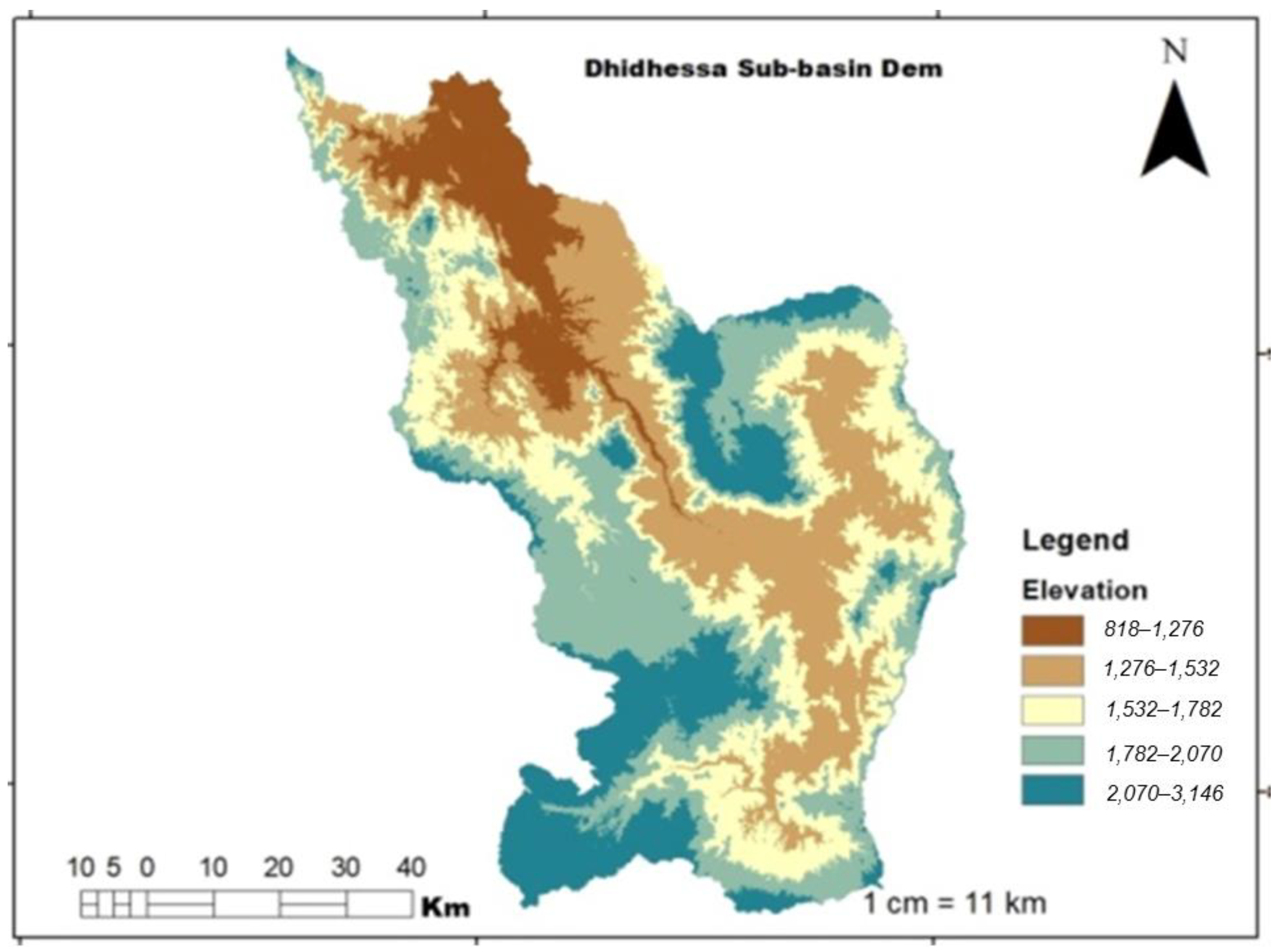
The elevation of the study area is between 818 m a.m.s.l. to 3146 m a.m.s.l, as depicted (Figure 2). The watershed primarily covers the Kola and Weina Dega climate zones, according to the Ethiopian climate classification based on elevation (i.e., <500 m: Bereha, 500–1500/1800: Kola, 1500/1800–2300/2000). 2400: Weina Dega, 2300/2400–3200: Dega, and >3200: Wurch [15].
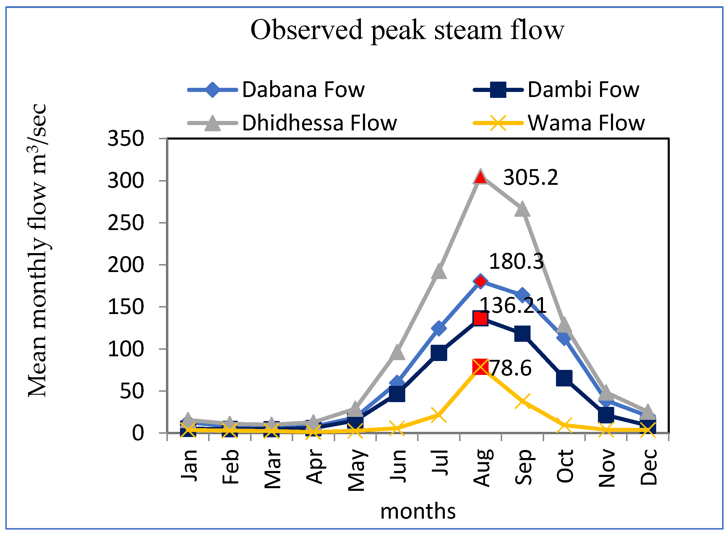
The Dhidhessa Sub-watershed is the largest of the Upper Blue Nile rivers with respect to water volume, contributing approximately a quarter of the total discharge as recorded at the Ethiopia–Sudan border alone [16]. Dabana near Bunoo Bedele, Dambi (Agaroo), Dhidhessa near Arjoo, and Wama are the major catchment areas of the discharge of the Dhidhessa Basin (Figure 3), indicating a rise in stream discharge. The Wama River enters the Dhidhessa River from the northeast, with a watershed of about 3767 km2, the Dabana flows from west to east, then north, near Bunoo Bedele, until it joins the Wama River. The Dabana sub-catchment near Bunoo Bedele is estimated to be around 4842 km2. Figure 3 portrays the statistical analysis of observed stream data from 1991 to 2020, depicting the maximum peak flow record in August.
The Dhidhessa catchment was delineated using a digital elevation model (DEM) with a resolution of 20 m × 20 m from the GIS Division of the Ministry of Water, Irrigation, and Energy (MoWIE). All LULC maps and data sets were collected in shape file format from the GIS Department of the Ministry of Water, Irrigation, and Energy (MoWIE). For the SWAT database/map window, the land use map was reclassified to display land use based on specific LULC types and corresponding crop parameters. To associate SWAT class grid values with LULC, a view was created from the map window database that defines the SWAT land use code for each LULC type.
Land use classes in the study area are Agricultural Land: Generic (AGRL), Agricultural-Row-Cropland (AGRR), Banana (BANA), Coffee (COFF), Forest-Deciduous-Leafy (FRSD), Forest-Evergreen (FRSE), Mixed Forest (FRST), Pasture (PAST), Range-Grasses (RNGE), Urban (URBN), Wetland-Forest (WETF), Wetland-Mixed (WETL), and Wetland-Forest Not Having (WETN). Agricultural Land: The generic covers a large area within this land use classification, as indicated by (Figure 4). The FAO/Globe soil classification system is used to classify consumer soils from the map window database in the study sub-basin. Soil types in the sub-basin sedimentation are discussed in the following section.
The major soil types considered in the study area include sub-basin sedimentation Cambisols, District Cambisols, Eutric Leptosols, Eutric Leptosols, Eutric Regosols, Eutric Vertisols, Haplic Acrysols, Haplic Alisols, Haplic Nitosols, and Rhodic Nitosols were considered in the study, according to the FAO. (Figure 4) indicates that Haplic Alisols are the most abundant soils in the study area and covered the area of the sub-basin as indicated by (Figure 5).

2.2. Methodology

2.2.1. Data Collection and Use

Meteorological, Hydrological, and Topographical Data

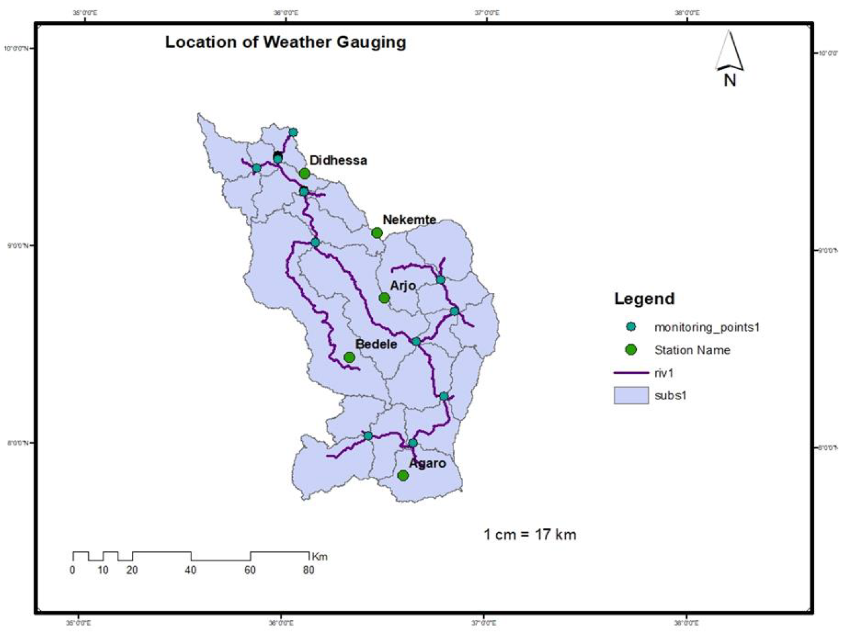
Precipitation, maximum and minimum temperature, relative humidity, wind speed, and solar radiation at five representative stations in the sub basin (Agaroo, Arjoo, Bedele, Dhidhessa, and Nekemte) were observed daily and meteorological data were continuously collected for a period of 30 years (1991–2020) from the National Meteorological Agency of Ethiopia (NMAE). The CORDEX Africa dataset is a database of future climate data for the years 2010 to 2099. CORDEX models were used to simulate monthly precipitation, min temperature, and max temperature from http://www.ccafs-climate.org/data_spatial_downscaling/ accessed on 1 June 2022. Stream flow data were collected from the Dhidhessa rain gauge stations (1991–2020) and GIS databases of the Ministry of Water, Irrigation, and Energy of Ethiopia (MoWIEE) Hydrology and GIS Department, respectively, for surface water evaluation in the basin as indicated by Table 1.
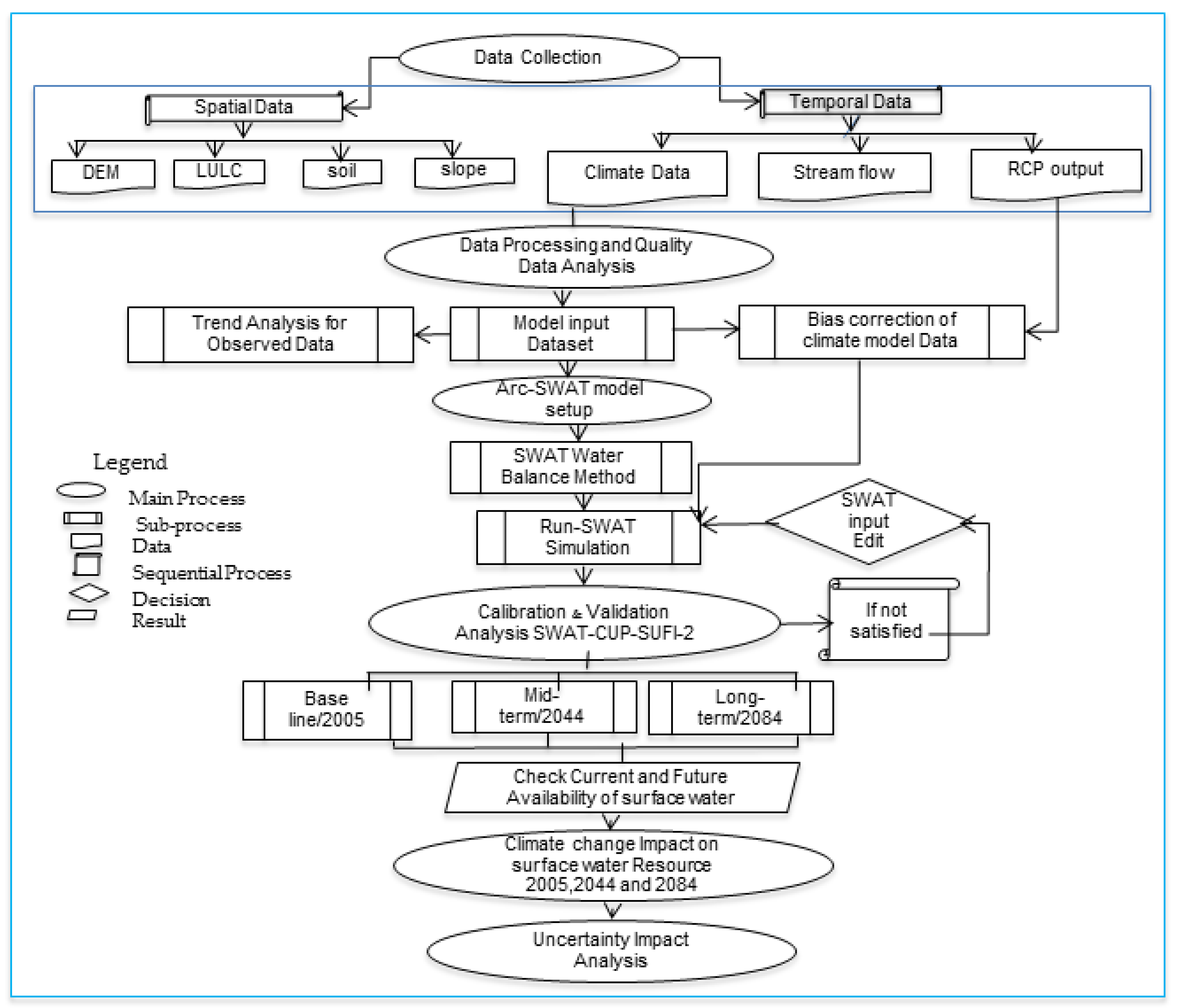
Soil and Water Assessment Tool (SWAT) simulations were used to assess surface water availability. This is a semi-distributed model that can be used to simulate the effects of climate change on stream flow and many other presences at the small-water scale. Specific input data, such as climate, hydrology, and spatial data must be used. Spatial data were processed using GIS Tools, which provided an interface to the SWAT model as both. GIS version 10.3 and SWAT 2012 were used in this study. Stochastic Uncertain Fitted, Version 2 (SUFI-2) is a parameter and model uncertainty analysis program integrated with the standalone program SWAT Calibration and Error Tool (SWAT-CUP) as indicated by Figure 6.

2.3. Basin Future Climate Change Scenario and the Selected Model

Each model has its advantages and disadvantages [17,18]. The performance of each model used in the study was compared to observation to attain this specific objective. The performance of an ensemble of models was also computed and compared to the models’ performance vs. the observation. This study used climate data from high-resolution regional climate models from the CORDEX-Africa database [19,20]. The driving model or GCMs are chosen based on earlier research or studies conducted in the Dhidhessa River Sub-basin [16,18]. As a result, the (Danish Hydrologic Institute) DMI-HIRHAM5, (Regional Atmospheric Climate Model Version 2.2) KNMI-RACMO22T, and (Swedish Meteorological and Hydrological Institute) SMHI-RCA4 driving models were chosen, and downscaling was performed using the most recent version of the regional climate model (RCM/RCP) gridded at 0.5° × 0.5° spatial resolution. When compared to regional climate models (RCM), most previous Upper Blue Nile (UBN) studies used GCMs, which have coarse resolution (RCM). GCMs are typically run at horizontal resolutions of 250–600 km, which is insufficient for evaluating local impact. Furthermore, previous studies relied on the SRES climate scenario, with only a few employing the newly developed representative concentration pathway scenario (RCPs). RCPs allow for the modeling of climate system responses to human activities, and they include data on a variety of long-lived GHGs, such as radioactively active gases and aerosol emissions, land use, and socioeconomic status. Some of the World Meteorological Organization’s (WMO) standard statistical metrics were used to compare model outputs to observations [21].
These statistics include bias, root mean square error, and coefficient of variation [22].
Bias = 1 N i = 1 N ( P i Obs i )
RMSE = 1 N i = 1 N ( P i Obs i ) 2
CV = i = 1 N ( P i   P ¯ ) ( Obs i Obs ¯ ) ( 1 N i = 1 N ( Obs i Obs ¯ ) 2 ) ( 1 N i = 1 N ( P i   P ¯ ) 2 )
The simulated and measured values are P and Obs, respectively, while the simulated and observed pairs are i and N.

Bias Correction

RCM models often have [23] significant biases when evaluated to observed data, even local downscaling to high resolution. Since these biases of rainfall and temperature were observed to vary spatially [24], bias corrections were performed for each sub-basin separately [24]. Temperature and rainfall data from climate models were bias-corrected at the sub-basin level in this study. The linear shifting and scaling method have been used to bias-correct the min and max temperatures by (Equation (1)) [18].
T Corrected = T mean   Obs + δ ( T Obs ) δ ( T RCM ) ( T RCM T mean   Obs ) + ( T mean   Obs T mean   RCM )
where TCorrected is the corrected daily temperature; T (mean Obs) is the mean observed temperature; T (mean RCM) is the mean simulated temperature; TRCM is the uncorrected daily temperature from the RCM model; TObs is the observed daily temperature; T (mean Obs) is the mean observed temperature, and T (mean RCM) is the mean simulated temperature. The modification was done separately to data from each of the 12 months [18].
A power transformation was used, which corrects both the coefficient of variation and the mean ([25]. Every daily rainfall quantity P is changed into a corrected P* using (Equation (2)) the following nonlinear correction:
P * = ap b  
where is the variable’s corrected value (rainfall) “b” is the scaling exponent, which is generated iteratively, and the RCM precipitation time series’ coefficient of variation equals that of the observed precipitation time series. After that, the constant “a” is determined to ensure that the mean of translated precipitation values equals the observed mean.
b = δ P   obs day μ P obs   day δ PRCM day μ PRCM day ,   P + = ( P RCM   day ) b ,   a = μ P   obs day μ P + RCM   day ,   and   P * = ( aP + ) b
δ = standard deviation, μ   = mean of the rainfall (RF), P + = corrected rainfall (RF), PRCM = Uncorrected rainfall (RF), P   obs = Observed rainfall (RF), and P * = Biasd rainfall (RF).

2.4. Hydrological Component of the SWAT Model

The hydrological component of the SWAT model is based on the water balance equation. Soil water, surface runoff, intercept, daily precipitation, evapotranspiration, percolation, lateral groundwater flow, return flow or base flow, snowmelt, transmission losses, and water production are all part of the SWAT model. Discharge from the vadose zone to deep water and base flow to and from deep water channels or base flow are the only factors considered for the hydrological model in SWAT. Groundwater from the deeper aquifer is not considered, because water reaching the deeper aquifer is assumed to contribute to stream flow at locations outside the reservoir. According to [26], surface runoff, lateral flow from the soil profile, and return flow or base flow from the deep aquifer all contribute to the water in the stream. Water discharged into shallow aquifers is considered lost from the watershed system and is therefore not included in the water assessment [27]. The soil water content of the catchment is calculated using (Equation (3)) below:
S Wt = S Wo + i = 1 t { R day Q Surf E a W Seep Q gw } i  
where SWt is the final soil water content (mm). SWo is the initial soil water content on day i (mm). t is the time (days). Rday is the amount of precipitation on day i (mm). Qsurf is the amount of surface runoff on day i (mm). Ea is the amount of evapotranspiration on day i (mm). Wseep is the amount of water entering the vadose zone from the soil profile on day i (mm); and Qgw is the amount of return flow on day i (mm). The water balance components in the SWAT model are calculated from the hydrological cycle and the equilibrium period/warm-up period using SWAT input time series temporal and spatial data as follows.

2.4.1. Surface Runoff

SWAT simulates surface runoff volumes and peak runoff rates for each HRU using daily or sub-daily rainfall amounts. The SCS curve number approach and the Green & Ampt infiltration method are two SWAT methods for evaluating surface runoff volume. The latter technique is more accurate in evaluating runoff volume, but it requires sub-daily time step data, which makes it nearly impossible to utilize in our nation. As a result, the SCS curve numbering approach was used. The general (Equation (4)) for the SCS curve number method is:
Q Surf = ( R day I a ) 2 ( R day I a + S )
where Qsurf is the accumulated runoff or rainfall excess (mm), Rday is the rainfall depth for the day (mm water), Ia is initial abstraction which includes surface storage, interception and infiltration prior to runoff (mm water), and S is retention parameter (mm water). The retention parameter S can be calculated by using (Equation (5)).
S = 25.4 × ( 1000 CN 10 )  
where CN is the curve number for the day and its value is the function of land use practice, soil permeability, and soil hydrologic group. The initial abstraction, Ia, is commonly approximated as 0.2S and (Equation (6)) becomes:
Q Surf = ( R day 0.2 S ) 2 R day + 0.8 S  

2.4.2. Peak Discharge

The peak volume flow rate past a specific location during a storm event is known as the peak discharge or peak surface runoff rate. The peak run-off rate is used to estimate sediment loss and water quality and is a measure of a storm’s erosive force. SWAT uses a modified rational method to compute the peak runoff rate (see Equation (7)) [28].
Q peak = CiA total 3.6  
where:
  • Qpeak is peak runoff rate (m3/s),
  • C is the runoff coefficient,
  • i is the rainfall intensity (mm/hr.),
  • Sub-basin area (km2) and 3.6 is conversion factor.

2.4.3. Water Yield

After the water balance system has been satisfied, the remaining total amount of water leaves each HRU and sub-basin and enters the main channel stream flow. SWAT calculates the total water yield contributes to stream flow in the reach as the net water passes through the HRU and sub-basin using the following equation:
WYID = SURQ + LATQ + GWQ TLOSS
where WYLD= water yield (mm) is the net amount of water that leaves HRU and the sub-basin and contributes to main channel stream flow, SURQ = surface runoff contribution to stream flow, LATQ = lateral flow contribution to stream flow (mm), GWQ = groundwater (base flow) from the shallow aquifer that enters the main channel (mm). TLOSS is a transmission loss (water lost from tributary channels and main channel bed loss (mm).

2.5. Evaluation of the SWAT Model Performance

For various simulations, performance data was used to evaluate whether calibration and validation periods, spatial and temporal ranges, and specific performance evaluation of calibrations were needed [28]. Calibration is a combination of manual and automated processes that evaluate parameters of the model that cannot be directly measured. The validation process evaluates if the model is working appropriately, and provides a framework for model calibration and validation that is systematic. The author of a previous study explains how to calibrate the SWAT model [28]. From 1991–2020, the model was in use for 30 years, and from 1994 to 2011, the watershed’s calibration was performed. Validation of the watershed was also completed for the years from 2012 to 2020. A model must fulfill all three of the following criteria to be considered for the chosen ensemble [28,29]. Three criteria were used in this study: the coefficient of determination (R2), the Nash–Sutcliffe Index (NSE), and the percent bias (PBIAS).

2.5.1. Coefficient of Determination (R2)

The coefficient of determination (R2) is a measure of how much variance in derived data the model experiences. The coefficient of determination (R2) is the most generally used parameter for evaluating a model’s performance, as depicted in the following (Equation (9)):
R 2 = { i = 1 n ( O i O mean ) ( P i P mean ) i = 1 n ( O i O mean ) 2 i = 1 n ( P i P mean ) 2 } .
where:
  • Oi denotes observed flow discharge at the time i,
  • Omean denotes average observed flow discharge,
  • Pi denotes simulated flow discharge at the time i,
  • Pmean denotes average simulated flow discharge, and n is the number of flow discharge data recorded. The (Table 2) depicts the performance rating R2 criteria defined by [29] for SWAT model calibration and validation.
  • R2 provides the strength of relation between observed and simulated values. Its value ranges from 0 to 1, a value close to 0 means very low correlation whereas a value close to 1 represents high correlation between observed and simulated discharge.

2.5.2. Simulation Coefficient of Nash—Sutcliffe (NSE)

The Nash–Sutcliffe simulation coefficient (NSE) measures how well the observed vs. simulated data plot fits the 1:1 line. A formula used to determine NSE is depicted in (Equation (10)).
NSE = 1 i = 1 n ( O i P i ) 2 i = 1 n ( O i O mean ) 2
Because of the classification, performance ratings for the NSE of this model are evaluated on multiple levels depicted by (Table 2) [28,29]. NSE determines the relative magnitude of the residual variance compared to the measured data. Its value ranges from −∞ to 1, where 1 indicates a perfect model and a value less than 0 indicates that the mean value of the observed time series would have been a better predictor than the model.

2.5.3. Percentage Bias (PBIAS)

PBIAS (percentage bias) determines whether the simulated data is larger or smaller than the observed data [28,29]. PBIAS results of (Table 2) indicate that the model simulation is in the correct ranges. Positive values indicate an underestimation of bias by the model, although negative values indicate over evaluation of bias by the model [30,31]. A formula used to determine PBIAS is depicted in (Equation (11)):
PBIAS = i = 1 n ( O i P i ) i = 1 n O i 100
For the evaluation of models, [32] assigned values of ENS, PBIAS, and R2 as the following (Table 2) depicts. It measures the difference between the simulated and observed quantity and its optimum value is 0. A positive value of the model represents underestimation, whereas a negative value represents the model overestimation.

3. Results and Discussion

3.1. Hydro-Meteorological Database Results

3.1.1. Test Analysis of Rainfall Trends in the Study Area

The Mann–Kendall trend test was used to evaluate for trends in precipitation and temperature data [33]. A test the null hypothesis that there is no trend in the data series, while the alternative hypothesis states that there is a trend in the time series. Mann–Kendall procedure tests were performed in XLSTAT (2015). Kendall’s Mann test seems to be a non-parametric method [34] that tests trends in time series without specifying linear or nonlinear trends, and is less susceptible to outliers [35]. The MK test has been widely used to identify important trends in hydro-meteorological time series data, and is usually promoted by the World Meteorological Organization (WMO) [36]. The test was performed with a 5% significance gate. In test interpretation, the p-value and Sen’s slope were the two most important variables. Such Mann–Kendall test statistics are provided in [33].
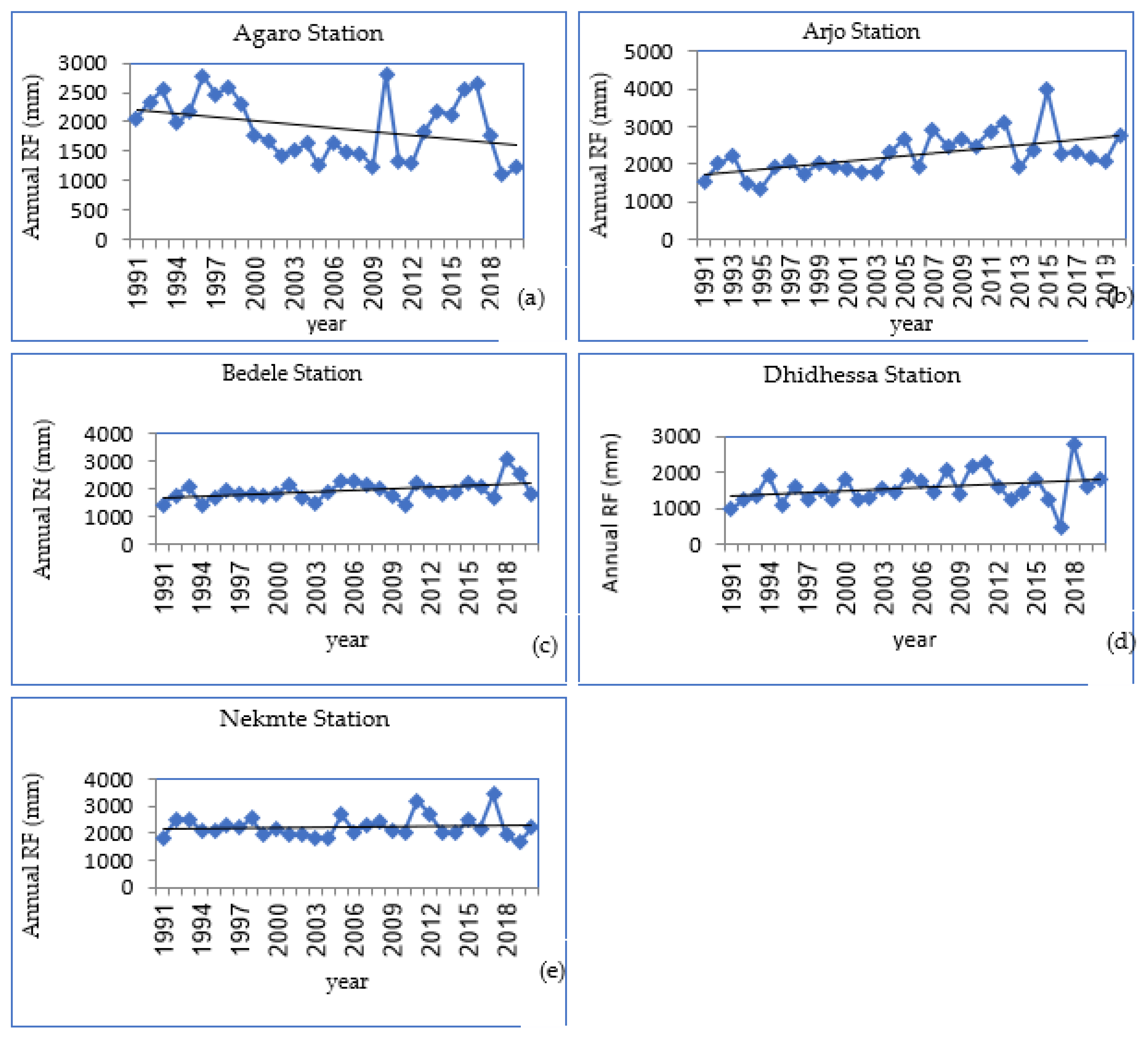
The Mann–Kendall test is a widely used nonparametric test for determining whether time series data have monotonic behavior [33]. The observed annual series of precipitation, temperature, and stream discharge of the Dhidhessa Sub-basin were evaluated using the non-parametric Kendall trend test with 5% significance level. The significance test in this study used a normalized p-value. When the p-value is small at the 0.05 alpha significance level, the null hypothesis should be rejected and the hypothesis accepted, and vice versa. (Table 3) depicts the estimated sens slope and Mann–Kendall trend test for rainfall for each site (Figure 7) and depicts the mean values for all Dhidhessa sub-catchment stations, the sens slope value, and the z value for rainfall. Figure 8 depicts the peak trend for Arjoo, Bedele, Dhidhessa, and Nekemte rainfall stations, but the worst trend for Agaroo. As indicated in (Table 3), the rate of change of annual precipitation is highest at Arjo station (2.2), and lowest at Agaroo station (2.0).

3.1.2. Test Temperature Trend Analysis on the Study Area

Long-term trends in the observed and adjusted time series data were identified using the MK test, with linear evolution of the data represented by Kendall–Theil Robust Lines. This non-parametric MK test is very suitable for assessing the variability of hydrological systems. Trend analysis was used to examine whether there was an upward, downward, or no trend in the value points of the data. This paper also used ITAM to identify time series data trends in precipitation, temperature, and runoff. To assess the reliability of the ITAM, the test results were compared with MK and Sen’s cross-sectional estimates.
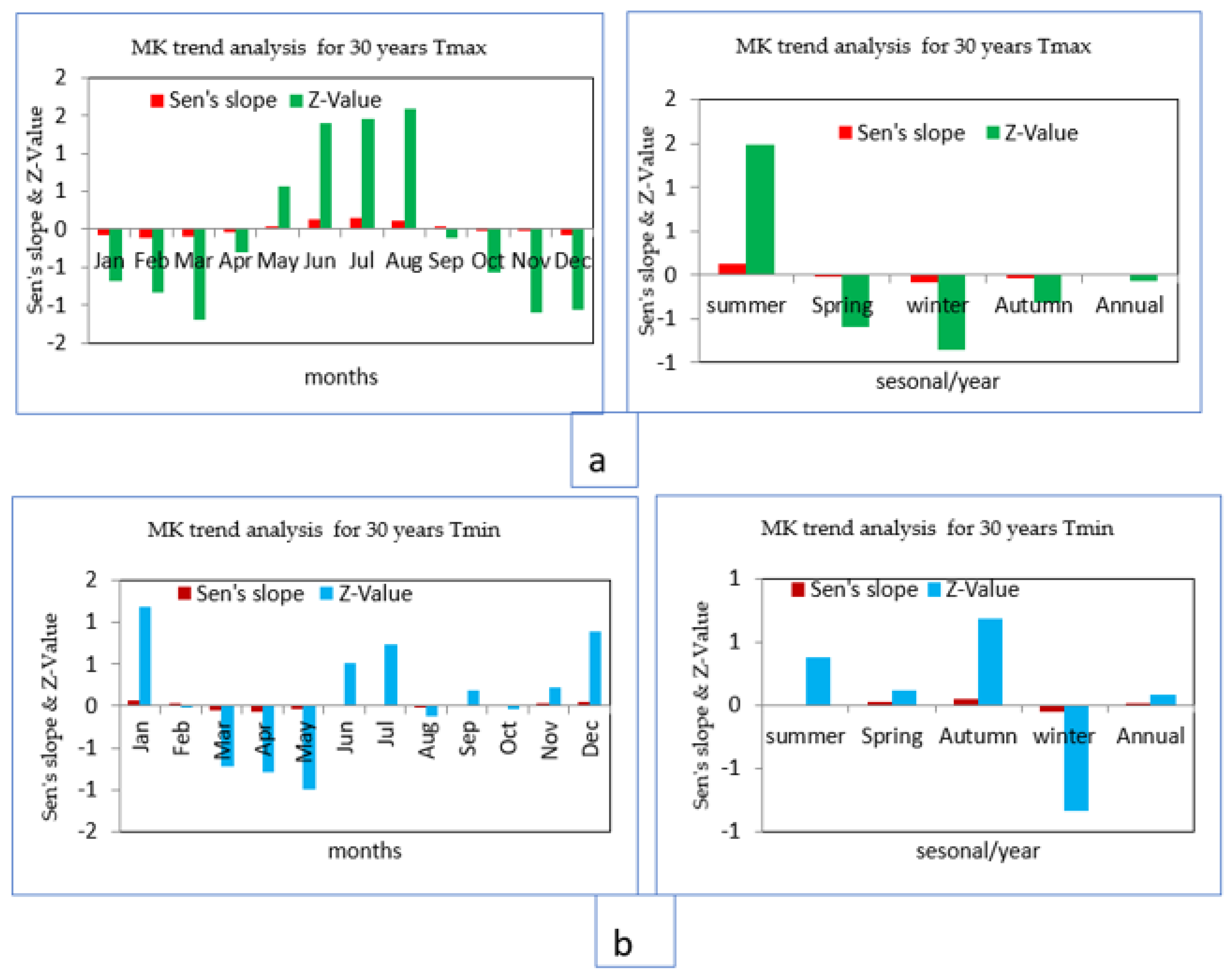
Annual min and max temperatures in the Dhidhessa Sub-basin (1991 to 2020) increased by 0.06 °C and 0.15 °C, respectively. The annual temperature in this sub basin has risen at a rate of 0.11 °C per decade. As depicted in the exhibit (Figure 9), while the average maximum temperature is increasing by 0.11 °C per decade, the average minimum temperature is decreasing by 0.07 °C per decade in the sub basin. The means of all stations, in addition to Sen’s slope and z-value, are depicted in (Table 4).
As a season, the maximum temperature in the study area increased by 0.1 °C in summer, while the maximum temperature in winter increased by 0.1 °C and the other two seasons by 0.0 °C in each year of the time series between 1991 to 2020 decreased. Similarly the minimum temperature of Dhidhessa Sub-basin depicted an increasing trend with a minimum value of 0.01 °C during summer, autumn and winter. The autumn season also decreased by 0.1 °C, and the maximum temperature of the Dhidhessa Sub-basin depicted a decreasing trend with minimum values of 0.034 °C, 0.004 °C, and 0.09 °C in autumn, winter, and spring, respectively; there is also an increased summer season, as depicted in (Figure 10a,b). In contrast to the other two seasons, the maximum temperature of the summer season demonstrated the highest increase of 0.1 °C per decade, while the minimum temperature of the autumn season depicted a decrease of 0.1 °C in value as (Table 4) in general, the variation of temperature is depicted in decades rather than in years.

3.1.3. Stream Flow Trends Test Analysis over the Study Area

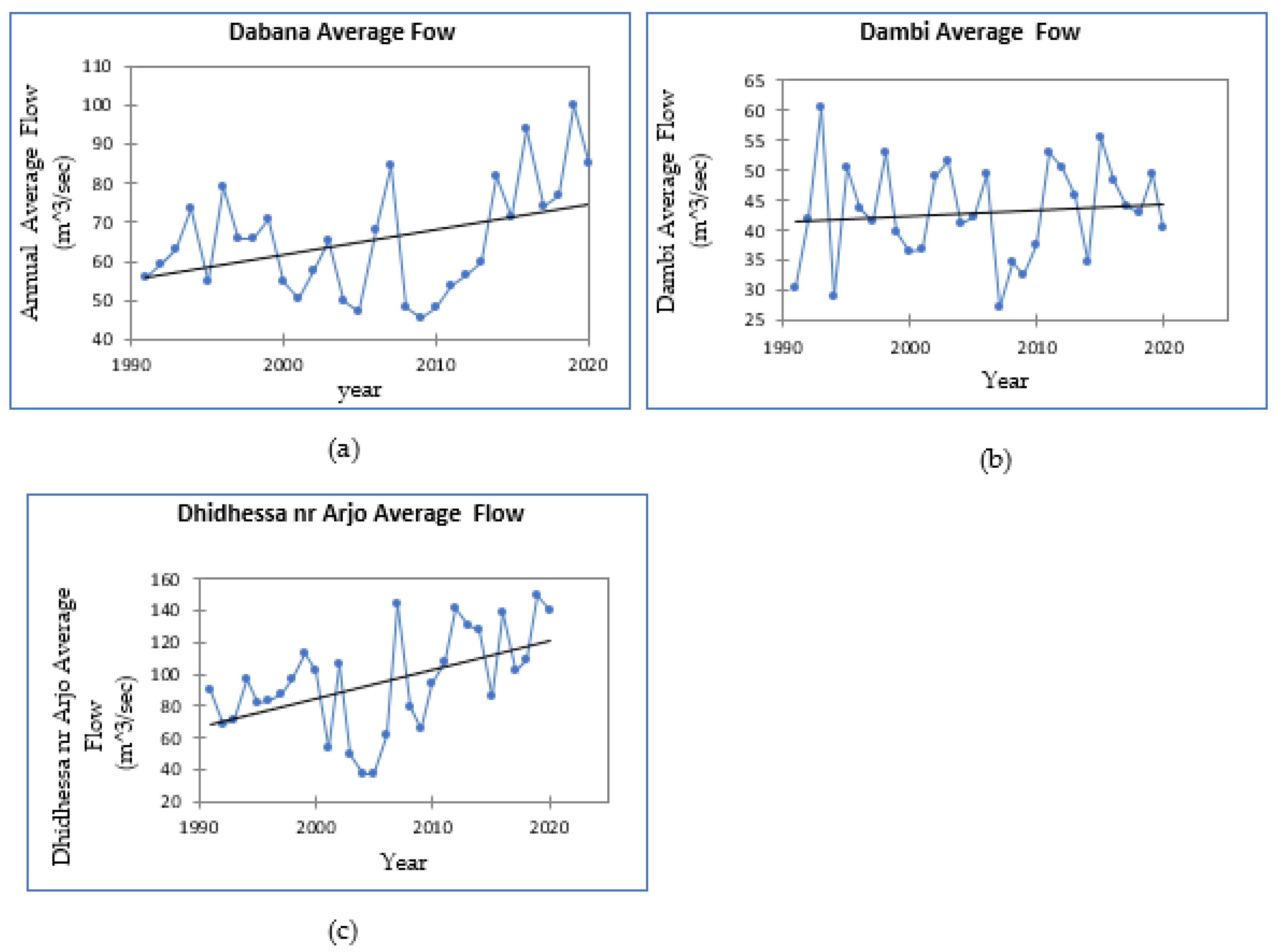
Trend analysis tests require the data to be sequentially independent. This is the primary factor that estimates parametric and nonparametric tests. Most studies of trend analysis have assumed that the recorded hydroclimatological time series are usually independent series, whereas some variables, such as annual mean data and low density, may indicate statistically significant serial correlation. The MK trend test in the Dhidhessa Sub-basin was on an annual time scale (i.e., p-value and Sen’s slope value) and was used to examine and identify trends that existed in the observed stream discharge data (Figure 11). With p-, a smaller decrease value is 0.724 and Sen’s slope is 7.542. The average annual amount exceeded each year from 1991 to 2020 decreased in value by 0.031 m3/s between each period and increased by 0.6 m3/s over the decade; the seasonal flow rate is depicted in (Figure 11).

3.2. Hydrological Modeling Result

Sensitivity Analysis

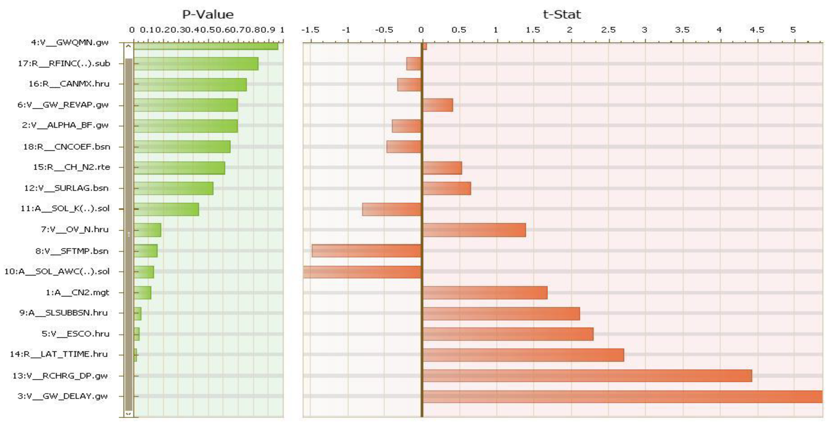
The sensitivity, calibration, and validation of the Dhidhessa SWAT hydrological model were performed at a multi gauge site (Dambi, Dabana near Buno Bedele, Dhidhessa near Arjo, and Wama). These were created using available measured climate and stream flow data and a popular algorithm called SUFI-2 to reduce the uncertainty in future predictions. The outcomes of the sensitivity analysis of global sensitivity (GSA) depicted several parameters which had direct relation and their impact on simulated stream flow resulted from the water yield remained after some losses passed through SWAT water balance systems depicted in (Figure 12). The most sensitive parameters were screened and ranked based on the absolute values of the t-stat and the positivity and negativity of the p-values of the GSA descriptive ranking, as depicted in (Figure 12). The GSA result indicted 18 most sensitive parameters and was regarded as relevant to water balance components such as precipitation, evapotranspiration, surface runoff, groundwater, and lateral flow, which directly affected the total water yield in the sub basin, as portrayed in the table below (Table 5).
The most sensitive parameters were CN2.mgt, GW_DELAY.gw, GWQMN.gw, ESCO.hru, GW_REVAP.gw, and OV_N.hru, followed by SLSUBBSN.hru ranked after repeated model iteration numbers. The daily curve number condition II (CN2.mgt) led the Dhidhessa SWAT model calibration system from the start to the end, particularly in controlling the direct surface runoff and total water yield (simulated stream flow). The overland flow parameter was Manning’s coefficient parameters (OV_N.hru), which also demonstrated a direct impact on simulated stream flow that started after saturated soil storage. The rainfall adjustment factor (RFINC (…).sub) parameters were applied at the sub-basins level to correct underestimated mean annual rainfall amount during the first simulation.
The increased and decreased value of this parameter depicted a direct relationship to simulated stream flow by increasing monthly rainfall amount. Manning’s coefficients (CH_N2.rte), which are used to limit the flow out rate (discharge) at the primary channel outlet, appear to be the most sensitive parameters in main channel routing. The surface lag time coefficient (SURLAG.bsn) is a surface runoff parameter that controls surface runoff by calculating concentration time from time travel and overland flow time. The deep recharging parameter (RCHRG_DP.gw) was used to control the ground water flow that returned as a return flow to the main channel stream flow. Because the deep aquifer recharge water increased as the value of this parameter increased, this was accounted for as a loss in the SWAT model throughout the calibration process. A detailed description of those relationships and their effects on calibrated monthly river discharge (discharge rate) and GSA sensitive parameter graphs can be found in (Table 5 and Figure 12).

3.3. Hydrological Model Calibration and Validation (SWAT)

3.3.1. Calibration Model

Once the sensitivity parameters for the model have been identified, the next step is to calibrate and validate the model. Both manual and automated measurement procedures (using the SUFI-2) were used in this study. Initially, the curve number for moisture condition II (CN2.mgt), aquifer delay time (GW_DELAY.gw), existing soil water potential (SOL_AWC (…).sol), and soil evapotranspiration compensation coefficient (ESCO.hru) are the calibration values that had been manually adjusted. For model calibration, we used Dhidhessa River data for 18 years (1994 to 2011) and validation (2012 to 2020) at each calibration station. Three years of data (1991–1993) were used for model warming. The performance of the model was evaluated for manual and automated calibration using R2, NES, and PBIAS statistical measures. The evaluation was performed on a monthly time scale, and the effect of statistical parameters obtained during measurement was 0.88 for R2, 0.76 for NES, and 2.41% for PBIAS. Flow density values indicate good agreement between observed and simulated. Figure 13 below depicts the hydrograph for comparison during model calibration.

3.3.2. Validation Model

Validation of model results is essential to enhance user confidence in model predictive capabilities. Nine years of monthly baseline data (2012–2020) were used for model validation without any adjustment of the fitted value during the calibration period, and values of 0.80 for R2, 0.77 for ENS, and 9.2% for PBias were obtained (Figure 13).

3.4. Evaluation of Surface Water Availability in the Present Climate

3.4.1. Monthly, Yearly, and Yearly Climate

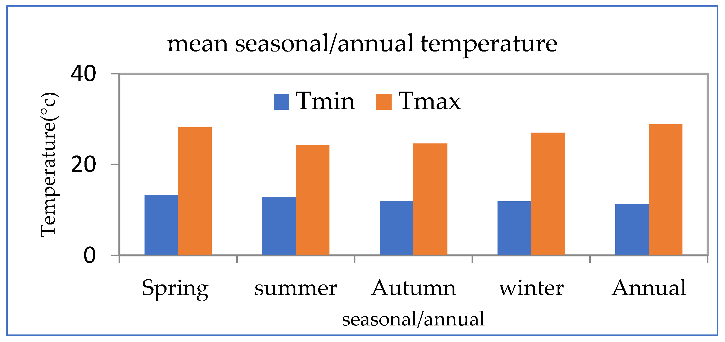
Figure 14 portrays the seasonal minimum, maximum, and mean Dhidhessa Sub-basin temperatures, mean annual temperatures, and climatic seasons (spring, summer, winter, and autumn). During this reference period (1991–2020), the mean monthly temperature of the sub-basin ranged from 11.25 °C to 28.84 °C, with a maximum and minimum monthly temperature of 20.98 °C found between 33.37 °C and 8.26 °C to 15.86 °C, respectively (Figure 14). Dhidhessa Sub-basin has annual minimum and maximum temperatures of 12.44 °C and 26.01 °C, respectively. Mean seasonal temperatures ranged from 12.74 to 24.25 °C, 11.89 to 24.6 °C, 11.82 to 27.01 °C, and 13.32 to 28.19 °C, (summer, autumn, winter, and autumn, respectively) between the minimum and maximum temperatures.

3.4.2. Water Balance Components of the Baseline Period (1991–2020)

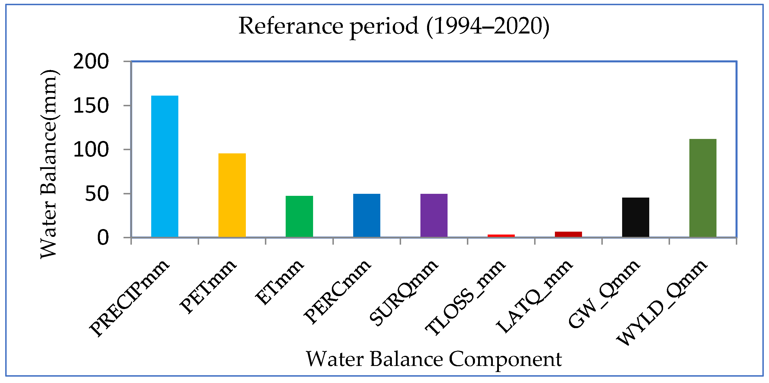
Most of the time, much water was lost as evaporation transmission and total losses, with 47.2 mm and 3 mm, respectively, of the mean annual rainfall captured over the Dhidhessa Sub-basin in the baseline period of 160.9 mm. The water yield retained as Dhidhessa current available water was 111.7 mm, as depicted in (Figure 15) below. The entire mean annual surface runoff as surface water availability was 57.3 mm of this total water production. The total amount of water that percolates down to the shallow and deep aquifers each year was 49.6 mm, with 6.7 mm of lateral flow and 45.2 mm of groundwater flow returning to the stream flow channel (Figure 15). The water that was permanently lost from the Dhidhessa Sub-basins was deep aquifer recharging and transmission losses, whereas the other water balance components were used in the hydrological cycle of the sub-basins. The mean annual potential evapotranspiration was estimated to be 95.5 mm in the sub-basin.

3.4.3. Monthly, Seasonal, and Annual Stream Flow under Current Climate

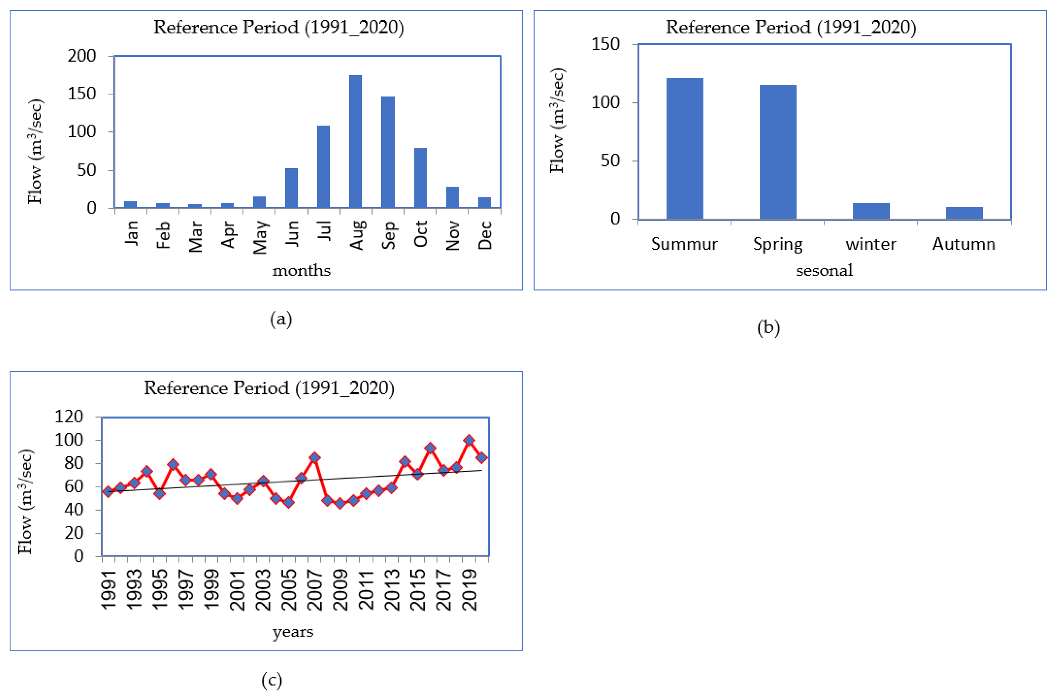
Figure 16 depicts the monthly, seasonal, and annual mean stream flow for the reference period (1991–2020). The rainy season months are August, September, and October, with peak flow rates of 324.6 m3/s, 347.8 m3/s, and 306.4 m3/s, respectively (Figure 16a). The summer and spring seasons in this study area are long, rainy, wet seasons, with maximum mean seasonal stream flow rates of 254.9 m3/s and 295.3 m3/s, respectively. The autumn season, which is a short rainy season with 81.7 m3/s, compared to a medium annual record and a low record in the winter (long dry) seasonal, as in (Figure 16b). The mean annual stream flow increased linearly from 1991 to 2020, with the highest flood occurring in 2019 with 100.1 m3/s and the lowest stream flow occurring in 2009 with 45.6 m3/s (Figure 16c).

3.5. Scenarios for Future Climate Change Signals

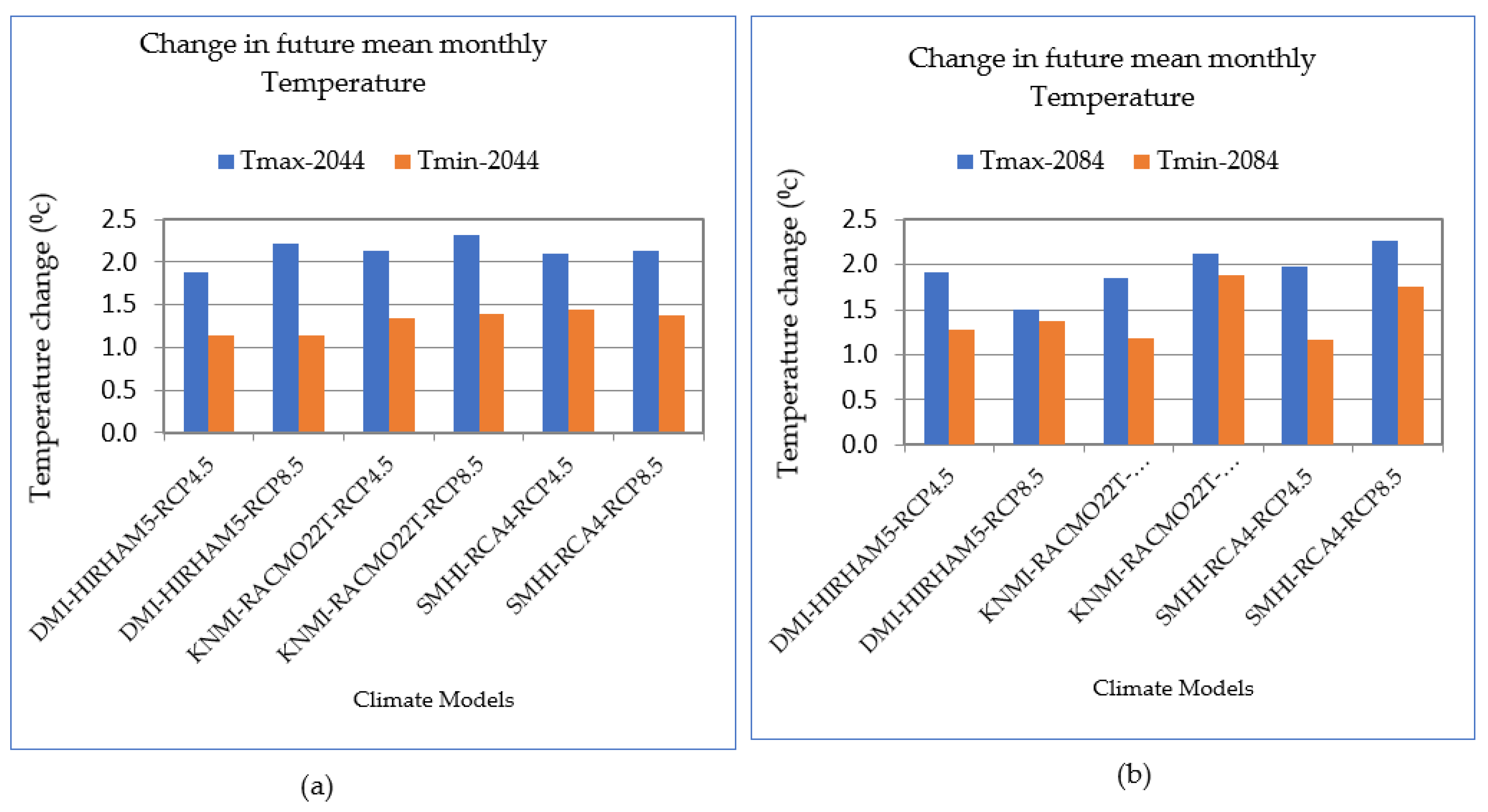
The change and trends detected monthly, seasonally, and annually of mean maximum and mean minimum temperature for each Representative Concentration Pathways (RCP) were summarized from a three-climate model (i.e., DMI-HIRHAM5, KNMI- RACMO22T, and SMHI-RCA4). The change in monthly mean temperature increased from 1.14 °C to 1.89 °C, 1.1 °C to 2.2 °C, 1.3 °C to 2.1 °C, 1.4 °C to 2.3 °C, 1.4 °C to 2.1 °C, and 1.4 °C to 2.1 °C, respectively, DMI-HIRHAM5-RCP4.5, DMI-HIRHAM5-RCP8.5, KNMI-RACMO22T-RCP4.5, KNMI-RACMO22T-RCP8.5, SMHI-RCA4-RCP4.5, and SMHI-RCA4-RCP8.5 in a short-term period (2044). In the long-term period (2084) was 1.3 °C to 1.9 °C, 1.4 °C to 1.5 °C, 1.2 °C to 1.9 °C, 1.9 °C to 2.1 °C, 1.2 °C to 2 °C, and 1.8 °C to 2.3 °C for RCP4.5 and RCP8.5, respectively, DMI-HIRHAM5-RCP4.5, DMI-HIRHAM5-RCP8.5, KNMI-RACMO22T-RCP4.5, KNMI-RACMO22T-RCP8.5, SMHI-RCA4-RCP4.5, and SMHI-RCA4-RCP8.5 (Figure 17a).
Although all months portrayed a considerable rise over their baseline period, there was a discrepancy across months and climate scenarios for both time frames. For example, the emission scenario (RCP8.5) depicted a significant change, while RCP4.5 depicted a low-significant increase over the long-term period of 2084 from the baseline period, and even in the long-term period of 2084 from January to March and July to September, RCP4.5 depicted a significant increase over the months under the RCP4.5 and RCP8.5 scenarios (Figure 17b).
Future mean monthly temperature changes for (a) RCP4.5, and RCP8.5 for 2044, (b) RCP4.5, and RCP8.5 for 2084 are depicted in (Figure 17). The monthly change in mean maximum temperature increased from 2.7 °C to 2.9 °C, 2.5 °C to 2.8 °C, 3.1 °C to 3 °C, 3.1 °C to 3.2 °C, 3.2 °C to 2.6 °C, and 3 °C to 2.9 °C, respectively DMI-HIRHAM5-RCP4.5, DMI-HIRHAM5-RCP8.5, KNMI-RACMO22T-RCP4.5, KNMI-RACMO22T-RCP8.5, SMHI-RCA4-RCP4.5, and SMHI-RCA4-RCP8.5 in the short-term period (2044). In the long-term period (2084) was 2.5 °C to 3.13 °C, 2.4 °C to 2.6 °C, 2.5 °C to 2.7 °C, 2.8 °C to 3 °C, 2.8 °C to 3 °C, and 3.1 °C to 3.4 °C for RCP4.5 and RCP8.5, respectively. The change in monthly mean minimum temperature increased from 1.44 °C to 1.45 °C, 1.2 °C to 1.7 °C, 1.4 °C to 1.6 °C, 1.1 °C to 1.4 °C, 1 °C to 1.6 °C and 1.3 °C to 1.8 °C, respectively, DMI-HIRHAM5-RCP4.5, DMI-HIRHAM5-RCP8.5, KNMI-RACMO22T-RCP4.5, KNMI-RACMO22T-RCP8.5, SMHI-RCA4-RCP4.5, and SMHI-RCA4-RCP8.5 in the short-term period (2044). In the long-term period (2084) was 1.2 °C to 1.9 °C, 1.5 °C to 2.1 °C, 1.4 °C to 1.6 °C, 1.7 °C to 2.4 °C, 1.2 °C to 2 °C and 1.2 °C to 2.4 °C for RCP4.5 and RCP8.5, respectively, DMI-HIRHAM5-RCP4.5, DMI-HIRHAM5-RCP8.5, KNMI-RACMO22T-RCP4.5, KNMI-RACMO22T-RCP8.5, SMHI-RCA4-RCP4.5, and SMHI-RCA4-RCP8.5, depicted in (Figure 17a). The change of mean temperature over the Dhidhessa in spring season, winter season and annually for the short-term period 2044 (Figure 18a), increased by 0.8 °C, 1.6 °C, and 0.3 °C, and summer and autumn season was decreased by 0.9 °C and 0.1 °C under intermediate emission RCP4.5 scenarios, respectively. Similarly, the short-term period of 2044 means temperature in spring season, winter season, and annual increased by 0.9 °C, 1.6 °C, and 0.3 °C, and summer, and autumn season was decreased by 1.0 °C, and 0.2 °C under high emission RCP8.5 scenarios, respectively, compared with the baseline period (Figure 18a). Under the long-term period (2084) (Figure 18b), the signal change of mean temperature in spring season, winter season, autumn season, and annually for the long-term period (2084) increased by 0.8 °C, 0.5 °C, 0.0 °C, and 0.2 °C, and the other in summer was decreased by 0.6 °C, under intermediate emission RCP4.5 scenarios, respectively. Similarly, the long-term period of 2084 means temperature in spring season, winter season, autumn season, and annual increased by 1.0 °C, 0.0 °C, 0.7 °C, and 0.3 °C, and the other in summer was decreased by 0.4 °C, under high-emission RCP8.5 (Figure 18) scenarios, respectively, compared with the baseline period.

3.6. Impact of Climate Change on Future Surface Water Availability

3.6.1. Future Components of the Water Balance

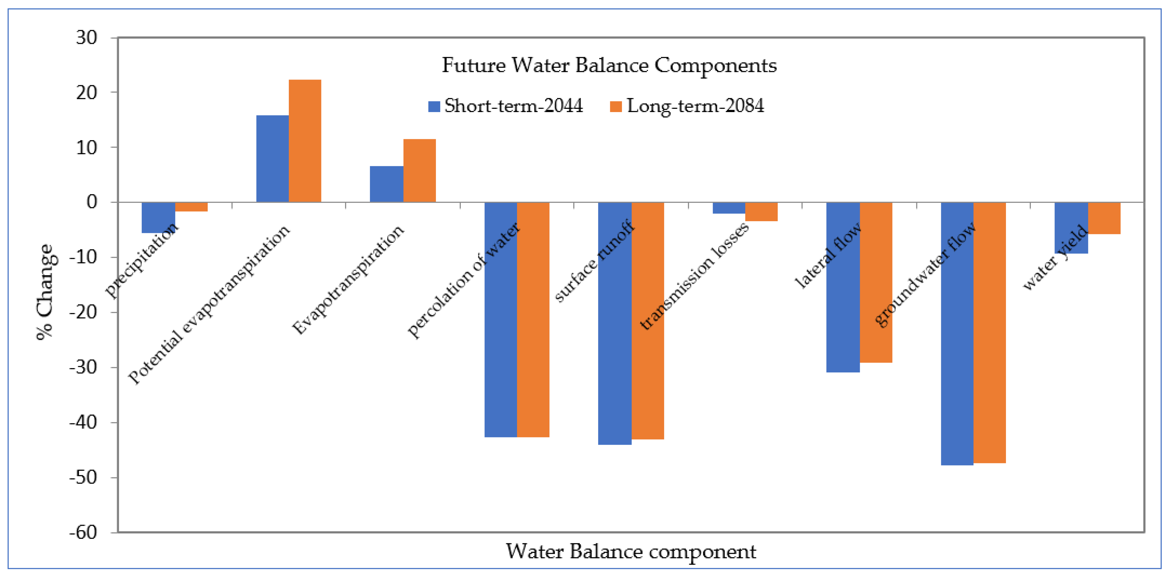
There is a mixed percent change for each water balance component from projected future climate scenarios at mean annual (i.e., 2044 (2030–2059) and 2084 (2070–2099) time steps over the Dhidhessa sub-basins modeled from a three-climate model under each RCP at a monthly time step. Under the shorter period (2044), the percent change in mean annual water balance components such as potential evapotranspiration and evapotranspiration increased insignificantly by 15.9%, and 6.5%, respectively, while precipitation, percolation of water, surface runoff, transmission losses, lateral flow, groundwater flow, and water yield dramatically decreased by 5.6%, 42.6%, 44%, 2.1%, 30.8%, 47.8%, and 9.2%, respectively. However, a significant decrease in change in return flow and lateral flow is due to a decrease in percent change in water percolation at the vadose root system. This percolation of water returned the total water yield from Dhidhessa to the main channel stream flow through the lateral and returns (groundwater) flow. This decreased percent change in total water production over the study region is a major issue for agricultural development and groundwater resource development in this sub-basin (Figure 19). Except for potential evapotranspiration and evapotranspiration, which increased by insignificant values with 22.4% and 11.6% change from the baseline period, all water balance components demonstrated an insignificant decrease in future percent change in the long-term period (2084), which is the same as the short-term period (2044). Under long-term period (2084) the percent change in mean annual water balance components such as precipitation, percolation of water, surface runoff, transmission losses, lateral flow, groundwater flow, and water yield was significantly reduced during this period, with 1.6%, 42.7%, 43.1%, 3.4%, 29.1%, 47.3%, and 5.7%, respectively, compared to the baseline period with compared the long-term period (2084).
The significantly reduced percent change in total water output will put agricultural development at risk, and domestic water supply will be scarce during this time, which will have a direct impact on livelihoods in the Dhidhessa Sub-basins. As depicted in (Figure 19), the potential evapotranspiration rose as a result of significantly higher trends in the mean annual temperature (2070–2099).
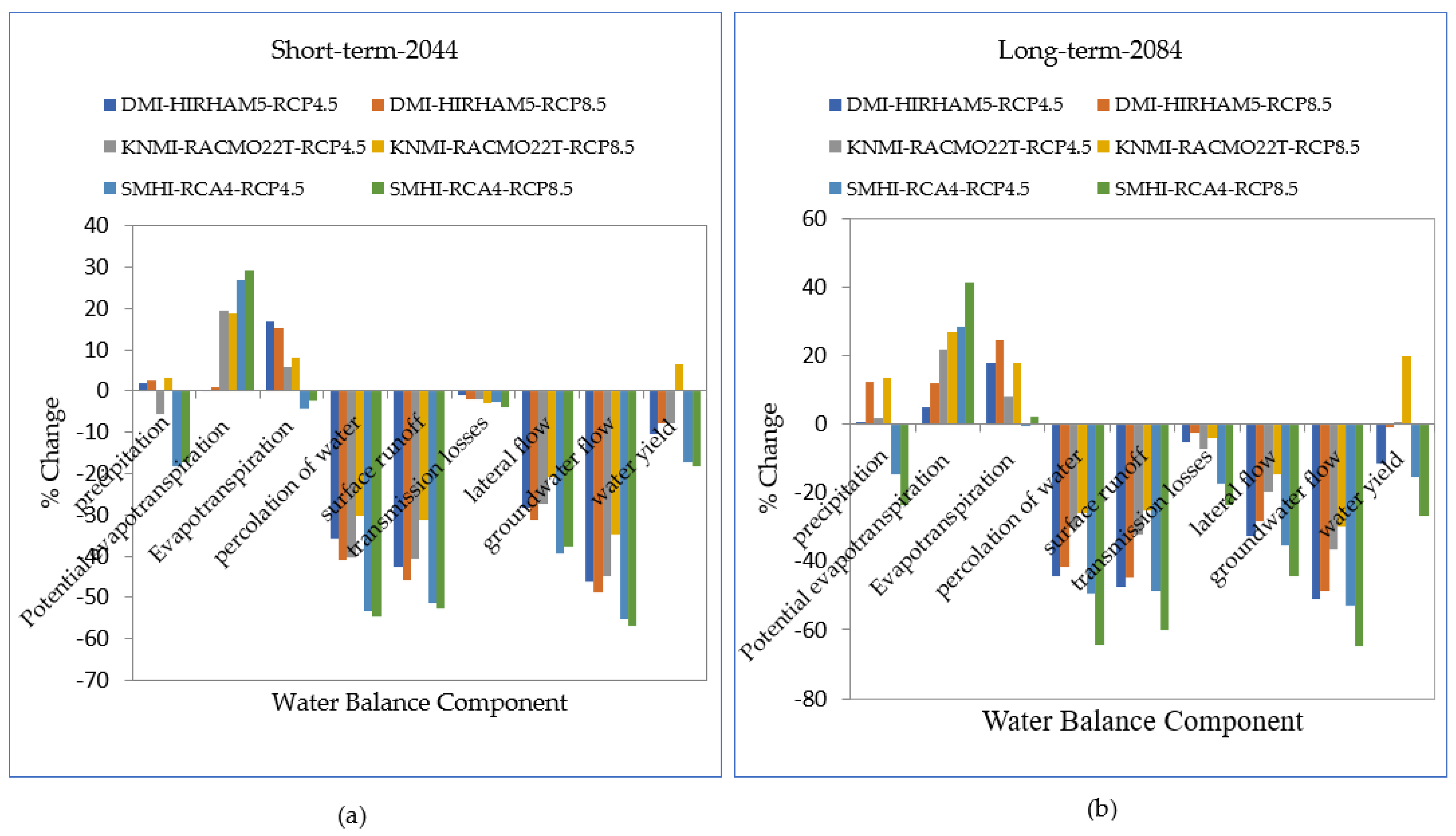
Except for potential evapotranspiration and evapotranspiration, all water balance components indicated a decreased percent change in the short-term period of 2044 under the emission scenario (RCP4.5). In the long-term period of 2084, there was a negative influence on the Dhidhessa Sub-basins, with all percent changes of future water balance components decreasing from baseline, except potential evapotranspiration and evapotranspiration, both strongly decreasing with percent change. Under this scenario, the decreased percent change in all components over the long run (2084) was the consequence of an increased percent change in potential evapotranspiration and evapotranspiration. Precipitation reduced by 5.6% and 1.6% in both periods (i.e., 2044 and 2084) respectively, percent change from the reference period (1991–2020) in this scenario (Figure 20). Potential evapotranspiration increased by 15.9% and evapotranspiration was also increased by 22.4% from the baseline period under the high-emission scenario (RCP8.5) (Figure 20) under short- and long-term periods, respectively.

3.6.2. Future Monthly Mean Flow

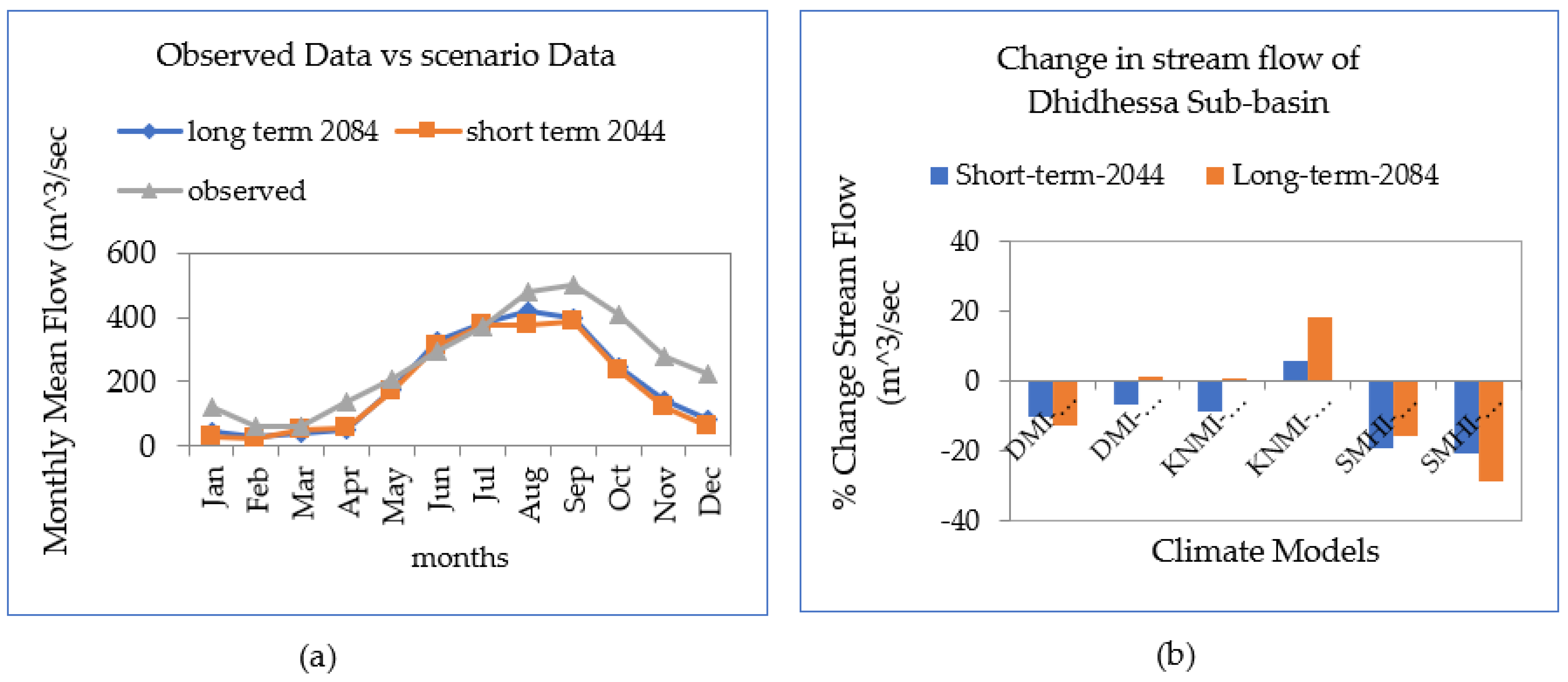
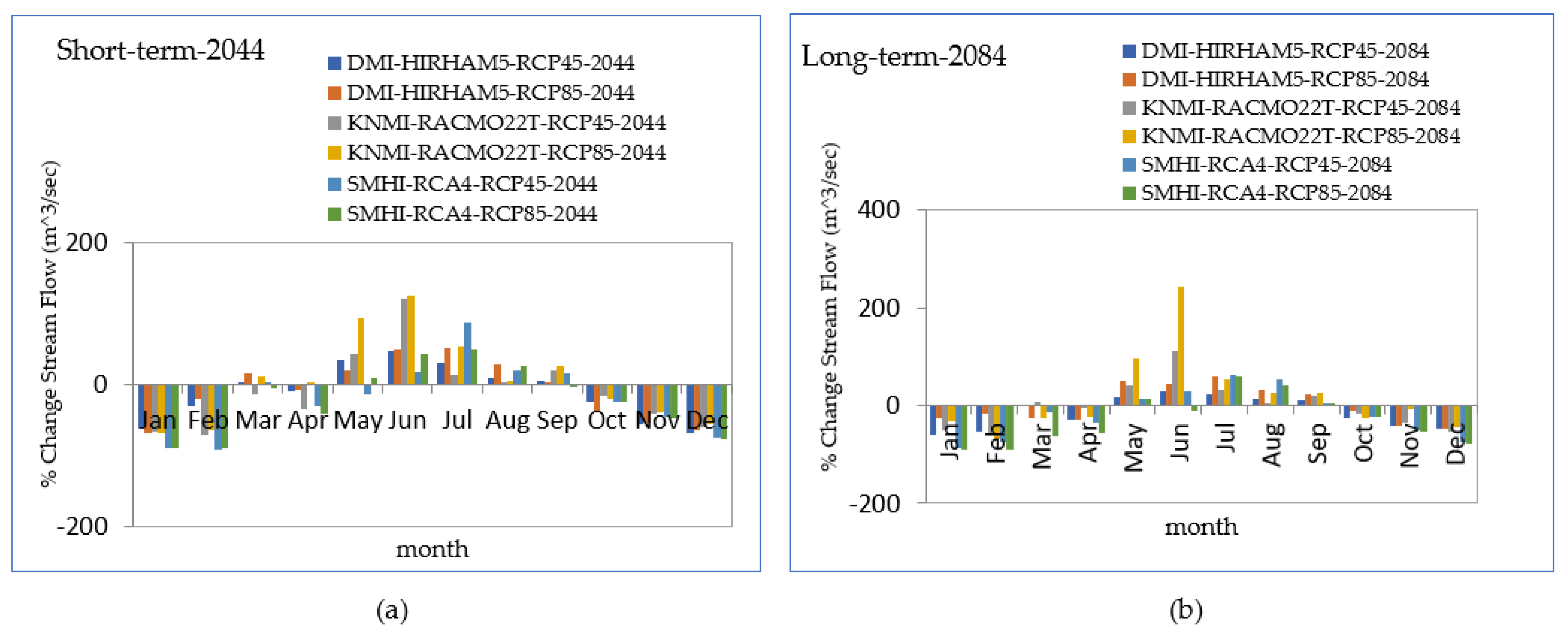
The month-flow rate modeled over (Dhidhessa Sub-basins) for two time periods (i.e., 2030–2059 and 2070–2099) revealed a mixed percent change from the reference period (1991–2020). Under the short-term period (2044) for models DMI-HIRHAM5-RCP4.5, DMI-HIRHAM5-RCP8.5, KNMI-RACMO22T-RCP4.5, SMHI-RCA4-RCP4.5, and SMHI-RCA4-RCP8.5, the mean stream flow percent change in the main channel river is decreased with 10.1%, 6.9%, 8.9%, 19%, and 20.7% from a baseline line period, respectively, but KNMI-RACMO22T-RCP8.5 model is increased by 5.7% insignificant. The decreased percent change in future stream flow in Dhidhessa Sub-basins is critical in case of survival of rain-fed agricultural production with supplementary irrigation system (spate and pump irrigation water).
Under the long-term period (2084), the mean stream flow over Dhidhessa Sub-basins exhibits a significant increase percent change for DMI-HIRHAM5-RCP8.5, KNMI-RACMO22T-RCP4.5, and KNMI-RACMO22T-RCP8.5 from their baseline period in opposite to short-term period increased by 1.2%, 0.7%, and 18.3%, respectively (Figure 21b). The 12.9%, 15.6%, and 28.6% decreases in % change over Dhidhessa Sub-basins in DMI-HIRHAM5-RCP 4.5, SMHI-RCA4-RCP4.5, and SMHI-RCA4-RCP8.5, respectively, resulted in a significant decrease in percent change from the baseline period (Figure 21b). Because the contribution of the Dhidhessa Sub-basins river comes from the steep slope area of the topography of the Dhidhessa watershed and other areas located around such a region, this significant decrease in future stream flow presents a difficult scenario in the socioeconomics of the study area.
With RCP4.5, the mean monthly stream flow for the long-term period (2084) will increase insignificantly from April to September, indicating the only considerable increase (72.1%) from the baseline period. The percentage change in these three situations will be minimal in January, February, March, April, October, November, and December, respectively. In March and May to September, the sub-basins will see a mild increase in the mean monthly percent change in stream flow, with a change interval of 2.3% to 124.5% change from their baseline period. The exceptional instance will be seen in the long-term period (2084) of RCP4.5, which will depict an inclination for months from May to September, with incremental percent change intervals ranging from 12.8% to 60.3%.
Generally, the RCP4.5 long-term period will experience a decreased change from January to April and October to December, with decrement intervals ranging from 12.6% to 89.2% and 22.9% to 74.3%, respectively, from the baseline period (1991–2020). For both periods (i.e., 2044 and 2084), the mean monthly future stream flow percent change under RCP8.5 demonstrates a mixed change from the baseline period, like RCP8.5 scenarios. In the short-term period (2044) of this scenario, the mean monthly stream flow of SMHI-RCA4-RCP4.5 percent change will prefer to swing between interval changes of −91.5% and 86.5%. February had the highest percentage loss with −91.5%, while July had the highest and most dominant shift with a large gain value (+86.5%) over the reference period (Figure 22).
Overall, this long-term period of RCP8.5 will experience a decline in change for KNMI-RACMO22T-RCP8.5, with changes ranging from minus 67.3 percent to 243.8 percent lower than the baseline period (1991–2020). During this time, the Dhidhessa Sub-basin’s main channel stream flow percent change will be at its lowest in February, at 67.3 percent, and at its highest in June, at 243.8 percent. The sub-basin stream flow will experience a minor reduction for the rest of this DMI-HIRHAM5-RCP8.5 scenario’s months in 2084, with a decrement interval of 46.5 percent to 59.5 percent (Figure 22b).

3.7. Monthly Flow for RCP Scenario

3.7.1. Average Seasonal and Yearly Flows in the Future Climate

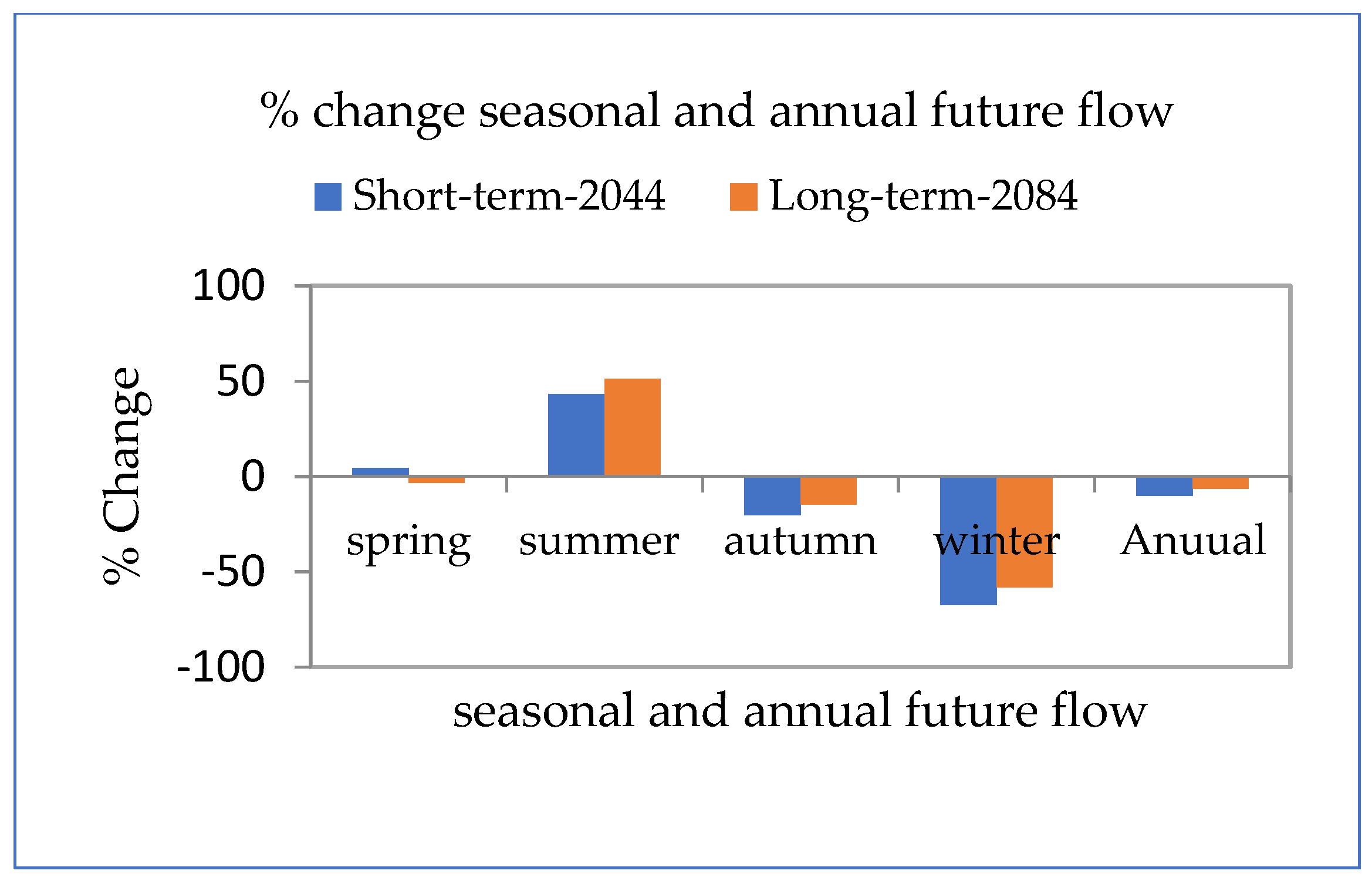
The Dhidhessa Sub-basins stream flow will undergo the maximum incremental percent change in both annual and seasonal periods (i.e., summer, spring, winter, and autumn). Stream flow significantly decreased in spring, winter, autumn, and annually with 20.2%, 67.4%, 67.4%, and 10%, respectively, while summer season increased by 43.1% in short-term from the baseline period (Figure 23). This lower-percent change in stream flow over this study area poses a risk to the sub-basin’s water sector development (Figure 23). The stream flow in the primary channel river over the Dhidhessa Sub-basin is expected to fail under the scarcity of water resource availability over the long-term period (2084). As depicted, (Figure 23) decreased in the following for both annual and three-season periods, except summer seasons, with 14.7%, 58.1%, 3.3%, and 6.3% change in spring, winter, autumn, and annually, respectively. And summer, with 51.1% from baseline, increased. The reduction in mean yearly water supply resulted in a considerable decrease in average yearly flow throughout this period.

3.7.2. Analysis of Uncertainties

Uncertainties in projected changes in the hydrological system arise from the following:
(1)
internal variability of the climate system
(2)
uncertainty in future greenhouse gas,
(3)
the translation of these emissions into climate change by GCMs/RCMs,
(4)
hydrological model uncertainty,
(5)
uncertainty from insufficient field data at all scales ([37]), and
(6)
uncertainty of downscaling techniques [38].
Generally, the sources of uncertainties of climate scenarios are multiple. The climate system itself is too complex to be represented in a numerical model and contains a number of assumptions and parameterizations that each climate modeling center approaches differently. Uncertainties in climate scenarios and RCM/RCP outputs may be large [39]. The uncertainties related to SWAT model in this work could be as follows: (1) the relationship between the predictor and predict and is achieved by only considering the data statistical condition, i.e., the model does not take into consideration the physical nature of the catchments (major drawback), (2) it requires high-quality data for model calibration; and (3) the model is highly sensitive to the choice of predictor variables and empirical transfer scheme. Parameter uncertainties and structural deficiencies in the hydrological models that are used for impact assessments are other sources of uncertainties [40,41]. This is why different hydrological models may provide different stream flow results for a given input [39].
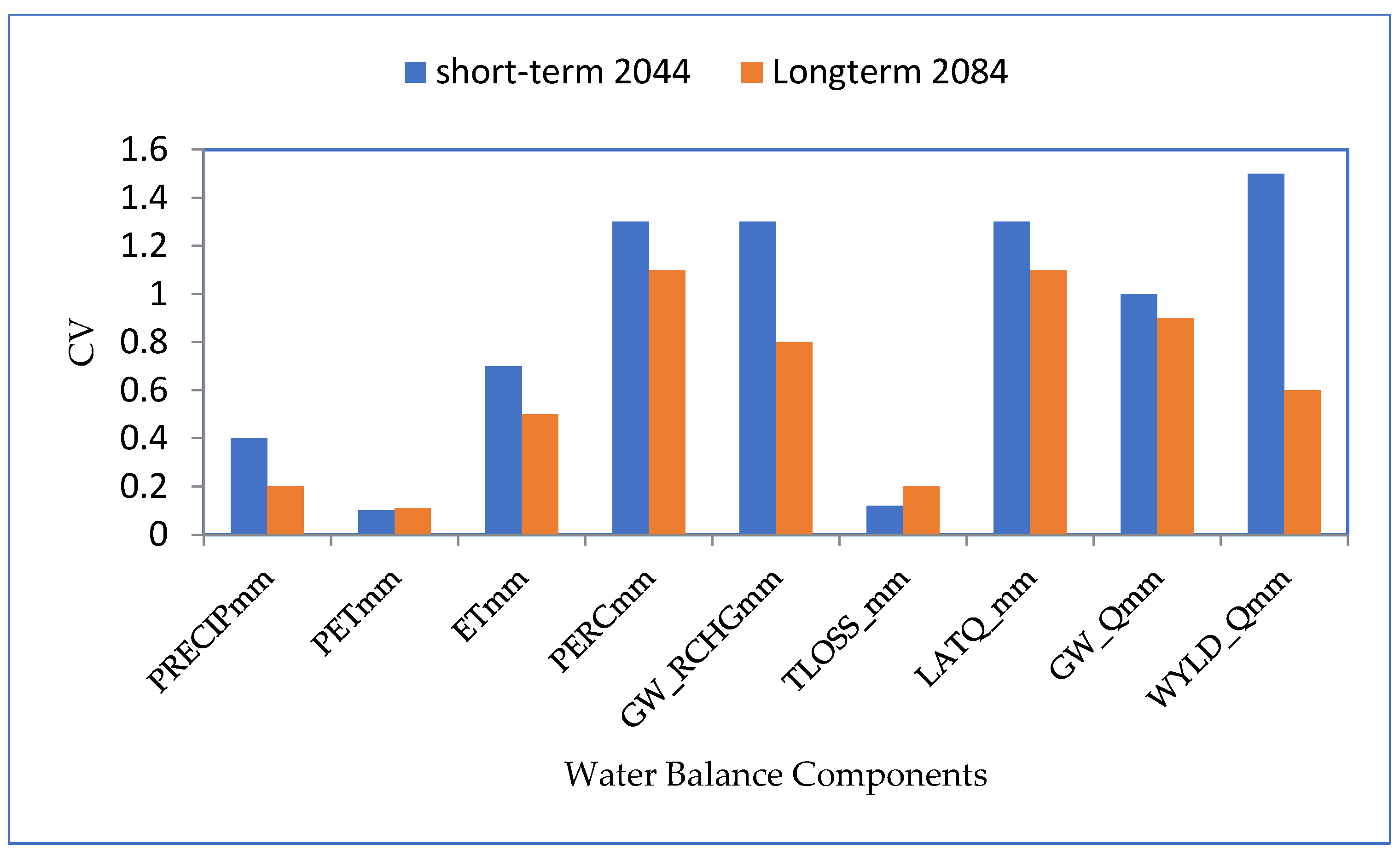
The study area uncertainties are increases in the short-term scenarios (2044) and a slight shift in the rainfall coefficient variation of the long-term future scenario (2084); the coefficient variation of the yearly distribution of rainfall and evapotranspiration in the sub-basins for the future scenario is largely identical to that of the baseline scenario (Figure 24). In general, the summer annual rainfall amount is lower in the long-term (2084) than in the baseline period, with less considerable uncertainty. The uncertainty of future mean annual surface runoff depth was high, with a rise in short-term coefficient variation (2044) balanced by a decrease in the long-term scenario (2084) from the baseline period.
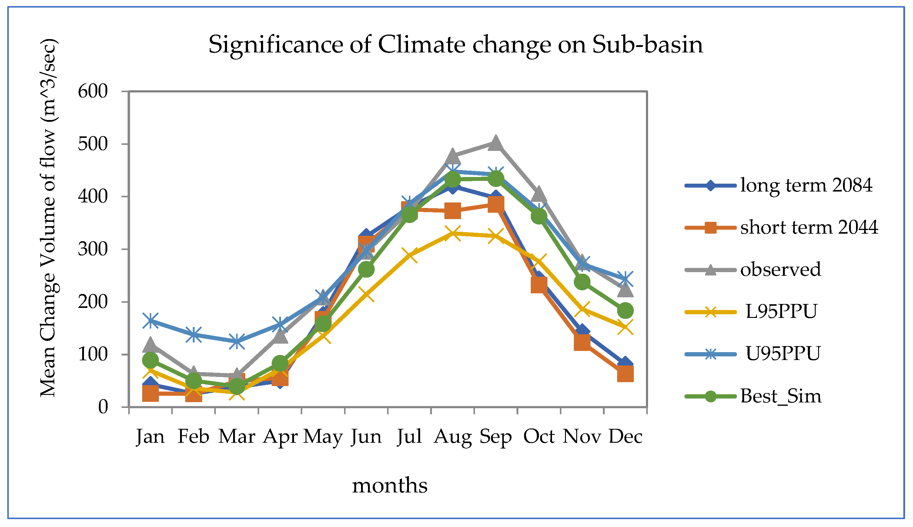
Figure 25 indicates whether hydrologic uncertainty is considerable for future generated runoff in the Dhidhessa Sub-basins. The discharge generated for the short term (2030–2059) was positioned between the two boundaries from January to June and September to November, indicating that the influence of climate change was minimal during this time (the change in discharge was because of other propagated uncertainty). However, hydrologic uncertainty was not expected for discharge created for the long-term scenario (2070–2099) from September to December because the discharge was generated outside of boundaries, indicating that the change in discharge was due to climate change. Therefore, the climate was relevant. In general, the generated discharge was placed outside of the two bounds; climate change influence is more significant in this sub-basin than the other propagated uncertainty on the amount of future runoff.
Previous studies in predicting climate change in the Upper Blue Nile River Basin are inconsistent for a variety of reasons. These include the length of both hydrological and metrological data, and the type of observed data used (gridded or station-based) in addition to the scale of the study area. Inconsistency is also owed to the geographical and temporal resolutions of observed and grid data sets, in addition to downscaling biased corrected output data for the simulation hydrology model and the scale of the study area’s range. Despite the aforementioned causes for uncertainty in future climate variable prediction over the Down Blue Nile River Basin, it is unclear which combination of inputs would provide a good insight for comprehending future possible climate conditions. In most of the studies cited, the current hydrological and meteorological parameter values are different. The majority of earlier investigations relied on gridded data sets, which were created by interpolating a few climate stations scattered over Ethiopia. To address mean annual and seasonal scale outcomes, statistical downscaling or bias correction approaches of GCM outputs based on SRES are frequently used. For this reason (RCP) gridded at 0.5° × 0.5° spatial resolution was latest one. For this reason, in such cases the recent RCP dataset used is crucial, and the value we obtained in this study is more accurate than the previous one when compared to the current situation.

4. Conclusions

Climate change jeopardizes national security and impedes the countries’ development. Climate change calls for immediate action. Water should be regarded as a natural resource that can have negative consequences when scarce. Water is necessary for the economic development of countries and the survival of living beings. Water is also required for food production, energy production, and ecosystem preservation. Climate change and water resource studies have been performed not only to protect and effectively use existing resources but also to identify the potential chained effects of various activities on ecosystems, in addition to the possibility of accelerating climate change. Damage to water resources should be avoided before it occurs. Before these damages endanger our personal, national, and global security, necessary steps must be taken. It should not be forgotten that carefully planned and consistently implemented policies would ensure a water-safe future. This study aims to evaluate the impact of climate change on the availability of surface water resources in the Dhidhessa Sub-basin and Lower Abbay Basin. The baseline period for the climate model framework is 1991 to 2020, and it is used to forecast future impacts in two time periods: 2030 to 2059 and 2070 to 2099, the short period being 2030–2059 and long-term period being 2070–2099, assuming a three-year warming period, Prior to using the SWAT model directly, bias correction was performed on the future precipitation and temperature datasets for the RCP4.5 scenario, yielding a bias-corrected RCM output of 4.5 watts per square meter (W/m2) and 8.5 watts per square meter (W/m2) for the RCP8.5 scenario. The average rainfall over the Dhidhessa Sub-basin decreased significantly between 1991 and 2020. The average annual precipitation in the spring declined dramatically, but it grew insignificantly in the summer, winter and autumn. The stream flow was observed to be significantly lowered during of the spring, but significantly higher in summers, winters, and autumn. The performance of Dhidhessa Sub-basins SWAT model calibrated and validated at the main; outlet Dhidhessa depicted very good performance with R2 > 0.75, NES > 0.75. This study also reproduced the performance of the SWAT Drift model which performed very well with stream flow R2 > 0.75 and NES value > 0.75. Overall, the model performance can be considered very good based on the percent of biased (PBIAS) capturing observed stream flow rates and hydrographic patterns. The change of mean temperature over the Dhidhessa in spring season, and winter season under the short-term period (2044), increased by 0.8 °C, and 1.6 °C, and the summer and autumn season was decreased by 0.9 °C, and 0.1 °C under this term and under intermediate emission RCP4.5 scenarios, respectively. Similarly, the short-term period of 2044 mean temperature in spring season, and winter season, increased by 0.9 °C, and 1.6 °C, and the summer, and autumn season was decreased by 1.0 °C, and 0.2 °C under high emission RCP8.5 scenarios, respectively, compared with the baseline period. Under the long-term period (2084), the signal change of mean temperature in spring season, winter season, autumn season, and annually increased by 0.8 °C, 0.5 °C, and 0.0 °C, and the other in summer was decreased by 0.6 °C, under intermediate emission RCP4.5 scenarios, respectively. Similarly, the short-term period of 2084 means temperature in spring season, winter season, autumn season, and annual increased by 1.0 °C, 0.0 °C, and 0.7 °C, and the other in summer was decreased by 0.4 °C, under high emission RCP8.5. The mean annual precipitations evaluated over Dhidhessa Sub-basins will likely reduce by 5.6% and 1.6% in both periods (i.e., 2044 and 2084) and under scenario RCP4.5 and RCP8.5, 1.66% and 1.71% respectively declined for the short-term period of 2044. Even if there is a difference between each scenario, with respect to the direction projected precipitation change, the long-term period of 2084 portrayed a declined trend with 2.5% RCP 8.5 while RCP 4.5 would experience the increased percent change of 4.7%. The mean annual total water yield predicted for Dhidhessa Sub-basins will experience a decrease by percent change with 9.2% for the short period of 2044 and a decline of 5.7% for 2084. Stream flow significantly decreased in spring, winter, autumn, and annually. According to the findings of this study, climate change can affect the availability of water in the Dhidhessa catchment. In this study, three climate models were used. The baseline (1991–2020), 2044s, and 2084s climate change scenarios were examined. The SWAT model was used to simulate rainfall runoff and generate future flow. All climate models’ projected changes in precipitation, temperature, and stream flow were concluded. In the 2044s, the annual rainfall in the Dhidhessa catchment is expected to change by 1.66 percent under RCP4.5 and 1.71 percent under RCP8.5. The annual rainfall will also change by 4.7% under RCP4.5 increased trend and 2.5% under RCP8.5 in 2084s decreased trend. In this study, multiple climate models were used to evaluate the impact on surface water source availability. This study also considers the ensemble mean of these various climate models. Scientists have been able to compare catchment level hydrological estimates to single-model projection, using multiple model ensembles. Many model ensembles, however, have yet to be used in Ethiopia and other parts of the world for research on their water resource potential in a changing climate scenario.

Author Contributions

Conceptualization, D.D.M.; methodology, D.D.M.; software, D.D.M.; Validation, D.D.M., D.A. and M.S.R.; system analysis, D.D.M.; research, D.D.M.; data processing, D.D.M.; preparation and writing first draft, D.D.M.; writing and editing the review, D.D.M., D.A., M.S.R. and M.K.L.; reveal, D.D.M.; control, D.D.M., D.A., M.S.R. and M.K.L. All authors have read and agreed to the published version of the manuscript.

Funding

This study received no external funding.

Institutional Review Board Statement

Not applicable.

Informed Consent Statement

Not applicable.

Data Availability Statement

The data used in this study can be obtained from the authors upon reasonable request.

Acknowledgments

The authors would like to thank the University of Rostock for their willingness to fund this publication under the Open Access Publication funding program.

Conflicts of Interest

The authors declare no conflict of interest.

References

  1. Opere, A.O.; Waswa, R.; Mutua, F.M. Assessing the Impacts of Climate Change on Surface Water Resources Using WEAP Model in Narok County, Kenya. Front. Water 2022, 3, 789340. [Google Scholar] [CrossRef]
  2. Salameh, E.; Abdallat, G. The Impacts of Climate Change on the Availability of Surface Water Resources in Jordan. J. Geosci. Environ. Prot. 2020, 8, 52–72. [Google Scholar] [CrossRef]
  3. EPA. The Effect of Climate Change on Water Resources and Programs. In Watershed Academy Web; U.S. Environmental Protection Agency: Washington, DC, USA, 2012. [Google Scholar]
  4. IPCC-TGICA. General Guidelines on the Use of Scenario Data for Climate Impact and Adaptation Assessment; Finnish Environment Institute: Helsinki, Finland, 2007; Volume 312, p. 66. [Google Scholar]
  5. IPCC. Climate Change 2001: The Scientific Basis. Contribution of Working Group I to the Third Assessment Report of the Intergovernmental Panel on Climate Change; Cambridge University Press: Cambridge, UK, 2001. [Google Scholar]
  6. Song, P.; Wang, C.; Ding, G.; Sun, J.; Kong, L.; Lu, M.; Lei, X.; Wang, H. Evaluating the impact of climate change on surface water resources in the upper Ganjiang River Basin, China. J. Water Clim. Chang. 2022, 13, 1462–1476. [Google Scholar] [CrossRef]
  7. Beker, H.J. Evaluation of Surface Water Resource Availability under Changing Climate Condition in the Erer-Mojo River Subbasin, Wabe-Shebele Basin; Arba Minch University: Arba Minch, Ethiopia, 2018. [Google Scholar]
  8. Mukheibir, P. Water access, water scarcity, and climate change. Environ. Manag. 2010, 45, 1027–1039. [Google Scholar] [CrossRef] [PubMed]
  9. IPCC. Climate Change 2007: The Physical Science Basis. Contribution of Working Group I to the Fourth Assessment Report of the Intergovernmental Panel on Climate Change; Cambridge University Press: Cambridge, UK; New York, NY, USA, 2007; p. 996. [Google Scholar]
  10. IPCC. Climate Change 2013: The Physical Science Basis. Contribution of Working Group I to the Fifth Assessment Report of the Intergovern- mental Panel on Climate Change; Cambridge University Press: Cambridge, UK; New York, NY, USA, 2013; p. 1535. [Google Scholar]
  11. Kiya, R. Impact of Climate Change on Water Resources. J. Earth Sci. Clim. Chang. 2014, 5, 185. [Google Scholar] [CrossRef]
  12. Chattopadhyay, S.; Jha, M.K. Climate Change Impact Assessment on Watershed Hydrology: A Comparison of Three Approaches. Am. J. Eng. Appl. Sci. 2014, 7, 122–128. [Google Scholar] [CrossRef]
  13. Ayivi, F.; Jha, M.K. International Soil and Water Conservation Research Estimation of water balance and water yield in the Reedy Fork-Buffalo Creek Watershed in North Carolina using SWAT. Int. Soil Water Conserv. Res. 2018, 6, 203–213. [Google Scholar] [CrossRef]
  14. Piao, S.; Ciais, P.; Huang, Y.; Shen, Z.; Peng, S.; Li, J.; Zhou, L.; Liu, H.; Ma, Y.; Ding, Y.; et al. The impacts of climate change on water resources and Crop Production in an Arid Region. Nature 2022, 467, 43–51. [Google Scholar] [CrossRef] [PubMed]
  15. MoA. Agro-Ecological Zones of Ethiopia; Ministry of Agriculture: Addis Ababa, Ethiopia, 1998.
  16. Bekele, W.T. Implication of Representative Concentration Pathway’s on Arjo-Didessa Catchment, Upper Blue Nile Basin, Using Multiple Climate Models; Arba Minch University: Arba Minch, Ethiopia, 2017. [Google Scholar]
  17. Endris, E.; Anitz, R.P.; Atthias, M.B.U. Assessment of the Performance of CORDEX Regional Climate Models in Simulating East African Rainfall. J. Clim. 2013, 26, 8453–8475. [Google Scholar] [CrossRef]
  18. Edamo, M.L.; Bushira, K.M.; Ukumo, T.Y.; Ayele, M.A.; Alaro, M.A.; Borko, H.B. Effect of climate change on water availability in Bilate catchment, Southern Ethiopia. Water Cycle 2022, 3, 86–99. [Google Scholar] [CrossRef]
  19. Kanoma, M.S.; Abdulkadir, M. The impact of future climate change on water availability in Gusau, Zamfara State, Nigeria. Dutse J. Pure Appl. Sci. 2022, 7, 144–154. [Google Scholar] [CrossRef]
  20. Hailemariam, K. Impact of climate change on the water resources of Awash River Basin, Ethiopia. Clim. Res. 1999, 12, 91–96. [Google Scholar] [CrossRef]
  21. Getahun, Y.S.; van Lanen, I.H.; Torfs, P.P. Impact of Climate Change on Hydrology of the Upper Awash River Basin (Ethiopia): Inter-Comparison of Old SRES and New RCP Scenarios. Ph.D. Thesis, Wageningen University, Wageningen, The Netherlands, 2014. [Google Scholar]
  22. Daba, M.H. Evaluating Potential Impacts of Climate Change on Hydro-meteorological Variables in Upper Blue Nile Basin, Ethiopia A Case Study of Finchaa Sub-basin Evaluating Potential Impacts of Climate Change on Hydro-meteorological Variables in Upper Blue Nile B. J. Environ. Earth Sci. 2018, 6, 48–57. [Google Scholar]
  23. Kefeni, K.; Mokonnen, B.; Roba, N. Evaluation the Performance of Regional Climate Models in Simulating Rainfall Characteristics over Upper Awash Sub-Basin, Ethiopia. Int. Res. J. Adv. Eng. Sci. 2020, 5, 134–138. [Google Scholar]
  24. Leander, R.; Buishand, T.A. Resampling of regional climate model output for the simulation of extreme river flows. J. Hydrol. 2007, 332, 487–496. [Google Scholar] [CrossRef]
  25. Terink, W.; Hurkmans, R.T.W.L.; Torfs, P.J.J.F.; Uijlenhoet, R. Evaluation of a bias correction method applied to downscaled precipitation and temperature reanalysis data for the Rhine basin. Hydrol. Earth Syst. Sci. 2010, 14, 687–703. [Google Scholar] [CrossRef]
  26. Setegn, S.G.; Rayner, D.; Melesse, A.M.; Dargahi, B.; Srinivasan, R. Impact of climate change on the hydroclimatology of Lake Tana Basin, Ethiopia. Water Resour. Res. 2011, 47, 1–13. [Google Scholar] [CrossRef]
  27. Neitsch, S.; Arnold, J.; Kiniry, J.; Williams, J. Soil & Water Assessment Tool Theoretical Documentation Version 2009; Texas Water Resources Institute: College Station, TX, USA, 2011; pp. 1–647. [Google Scholar] [CrossRef]
  28. Moriasi, D.N.; Gitau, M.W.; Pai, N.; Daggupati, P. Hydrologic and Water Quality Models: Performance Measures and Evaluation Criteria. Am. Soc. Agric. Biol. Eng. 2015, 58, 1763–1785. [Google Scholar]
  29. Xue-song, Z.; Fang-hua, H.A.O.; Hong-guang, C.; Dao-feng, L.I. Application of Swat Model in The Upstream Watershed of the Luohe River. Chin. Geogr. Sci. 2003, 13, 334–339. [Google Scholar]
  30. Mazengo, M.; Kifanyi, G.E.; Mutayoba, E.; Chilagane, N. Modeling Surface Water Availability for Irrigation Development in Mbarali River Sub-Catchment Mbeya, Tanzania. J. Geosci. Environ. Prot. 2022, 10, 1–14. [Google Scholar] [CrossRef]
  31. Liersch, S.; Tecklenburg, J.; Rust, H.; Dobler, A.; Fischer, M.; Kruschke, T.; Koch, H.; Hattermann, F.F. Are we using the right fuel to drive hydrological models ? A climate impact study in the Upper Blue Nile. Hydrol. Earth Syst. Sci. Discuss 2016, 22, 2163–2185. [Google Scholar] [CrossRef]
  32. Gupta, H.V.; Sorooshian, S.; Yapo, P.O. Status of Automatic Calibration for Hydrologic Models: Comparison with Multilevel Expert Calibration. J. Hydrol. Eng. 1999, 4, 135–143. [Google Scholar] [CrossRef]
  33. Fentaw, F.; Melesse, A.M.; Hailu, D.; Nigussie, A. Precipitation and streamflow Variability in Tekeze River Basin, Ethiopia; Elsevier Inc.: Amsterdam, The Netherlands, 2019; ISBN 9780128159989. [Google Scholar]
  34. Meena, M. Rainfall Statistical Trend and Variability Detection Using Mann- Kendall Test, Sen’s Slope and Coefficient of Variance—A Case Study of Udaipur District (1957–2016). Appl. Ecol. Environ. Sci. 2020, 8, 34–37. [Google Scholar] [CrossRef]
  35. Yue, S.; Wang, C. The Mann-Kendall Test Modified by Effective Sample Size to Detect Trend in Serially Correlated Hydrological Series. Water Resour. Manag. 2004, 18, 201–218. [Google Scholar] [CrossRef]
  36. WMO. World Climate Programme: Analyzing Long Time Series of Hydrological Data with Respect to Climate Variability; WMO/TD-No. 224; World Metrological Organization (WMO): Geneva, Switzerland, 1988. [Google Scholar]
  37. Masimba, O.; Gumindoga, W.; Mhizha, A.; Rwasoka, D.T. An assessment of baseline and downscaled projected climate variables in the Upper Manyame sub-catchment of Zimbabwe. Phys. Chem. Earth 2019, 114, 102788. [Google Scholar] [CrossRef]
  38. Zwiers, F.W. Global Increasing Trends in Annual Maximum Daily Precipitation. J. Clim. 2012, 26, 3904–3919. [Google Scholar] [CrossRef]
  39. Bourqui, M.; Mathevet, T.; Gailhard, J.; Hendrickx, F. Hydrological validation of statistical downscaling methods applied to climate model projections. IAHS-AISH Publ. 2011, 344, 32–38. [Google Scholar]
  40. Movahedinia, F. Assessing Hydro-Climatic Uncertainties on Hydropower Generation. Master’s Thesis, Laval University, Quebec, QC, Canada, 2014; pp. 1–50. [Google Scholar]
  41. Abdo, K.S.; Fiseha, B.M.; Rientjes, T.H.M.; Gieske, A.S.M.; Haile, A.T. Assessment of climate change impacts on the hydrology of Gilgel Abay catchment in Lake Tana basin, Ethiopia. Hydrol. Process. 2009, 23, 3661–3669. [Google Scholar] [CrossRef]
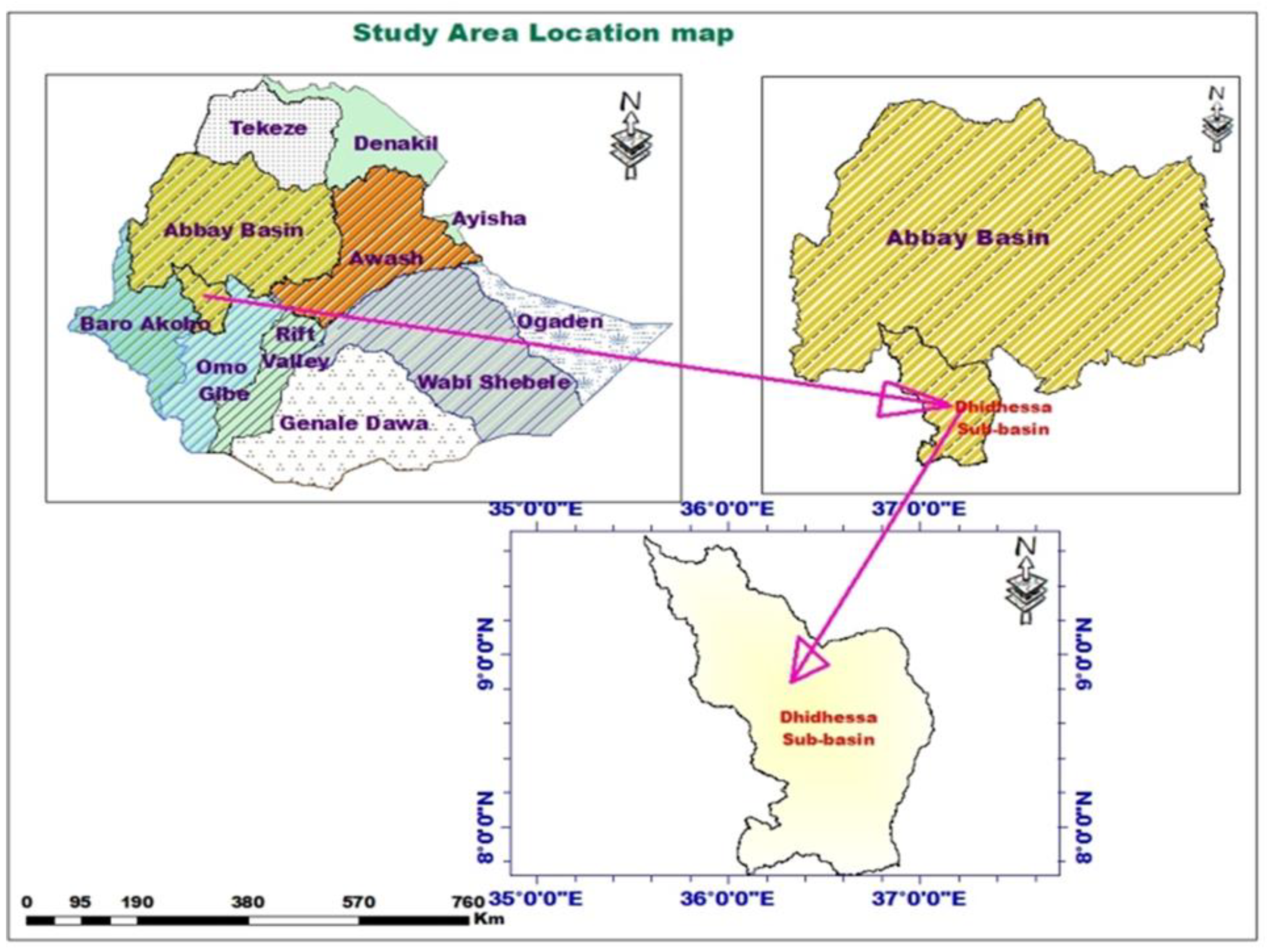
Figure 1. Location map of Dhidhessa Sub-basin.
Atmosphere 13 01296 g001
Figure 2. Topography of Dhidhessa Sub-basin.
Atmosphere 13 01296 g002
Figure 3. Peak Steam Flow of each gauge stations of the Catchments.
Atmosphere 13 01296 g003
Figure 4. Location of Gaging Stations.
Atmosphere 13 01296 g004
Figure 5. Land use/land cover (left) and soil map (right).
Atmosphere 13 01296 g005
Figure 6. Research methodology flow chart.
Atmosphere 13 01296 g006
Figure 7. Means values of stations for Sen’s slope value and Z-Value. (a) months, (b)seasonal/year.
Atmosphere 13 01296 g007
Figure 8. Trends of observed rainfall in (a) Agaro Station, (b) Arjo Station, (c) Bedele Station, (d) Dhidhessa Station, (e) Nekmte Station.
Atmosphere 13 01296 g008
Figure 9. (a) Tmax (b) Tmin, for means of Sen’s Slope Value, and z-value.
Atmosphere 13 01296 g009
Figure 10. Tmax (ae) and Tmin (bj) Trend Test Applied at Annual on Temperature.
Atmosphere 13 01296 g010
Figure 11. Trend test applied annually on observed stream-flow. (a) Dabana Average Flow, (b) Dami Average Flow, (c) Dhidhessa nr Arjo Average Flow.
Atmosphere 13 01296 g011
Figure 12. GSA sensitive parameters.
Atmosphere 13 01296 g012
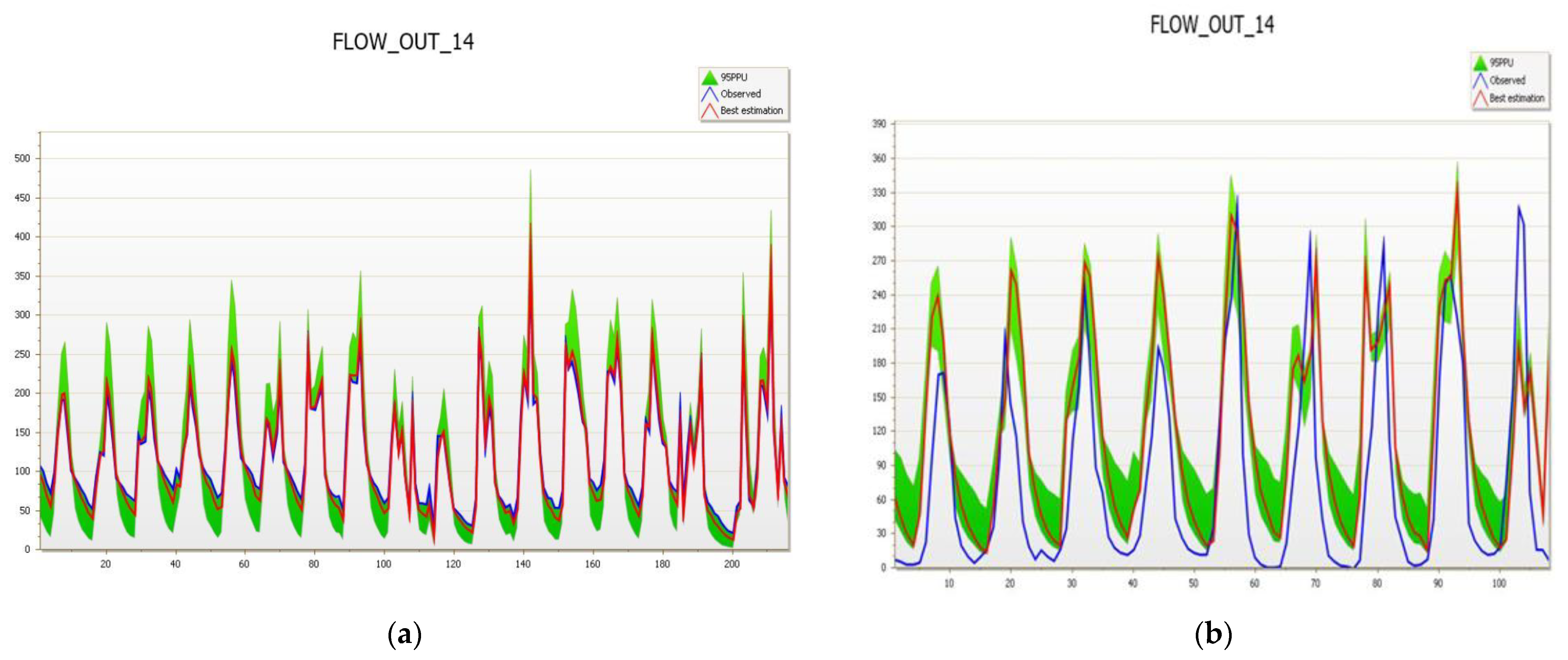
Figure 13. (a) Stream flow Calibration for Dabana Station and and (b) Stream flow Validation for Dabana Station.
Atmosphere 13 01296 g013
Figure 14. Relationship between mean seasonal max and min temperatures.
Atmosphere 13 01296 g014
Figure 15. Dhidhessa Sub-basins Average Annual Water Balance Components.
Atmosphere 13 01296 g015
Figure 16. (a) Monthly, (b) Seasonal, and (c) Annual Mean Stream flow.
Atmosphere 13 01296 g016
Figure 17. (a) 2044 and (b) 2084, Change in Future Mean Monthly Temp by two faces.
Atmosphere 13 01296 g017
Figure 18. (a) 2044 and (b) 2084; Change in Mean seasonal and annual future Temperature.
Atmosphere 13 01296 g018
Figure 19. Water balance components percent.
Atmosphere 13 01296 g019
Figure 20. Percent change in mean annual water balance components under two RCP scenarios: (a) 2044 and (b) 2084.
Atmosphere 13 01296 g020
Figure 21. Change in stream flow in the Dhidhessa Basin under scenarios from (a) 2044 (2030–2059) and (b) 2084 (2070–2099).
Atmosphere 13 01296 g021
Figure 22. (a) 2044 and (b) 2084; Percentage Change in Mean.
Atmosphere 13 01296 g022
Figure 23. Change in seasonal and annual future flow percentages from the baseline period.
Atmosphere 13 01296 g023
Figure 24. Coefficient variation in water balance components.
Atmosphere 13 01296 g024
Figure 25. Uncertainty in baseline and future flow rate.
Atmosphere 13 01296 g025
Table 1. Listed Weather Monitoring Stations.
Station NameZoneStation
Elevation
LatitudeLongitudeData
Coverage
% of
Missing
Rainfall
% of
Missing
Temp. (°C)
AgaroJimma16667.8536.61991–20202222.5
ArjoEast wollega25658.7536.51991–20202137.5
BedeleIllubabor20118.4536.331991–20202117.5
DidhessaEast wollega13109.3836.11991–20202046
NekemteEast wollega20809.0836.461991–20202120.5
Table 2. Classification of indices under the calibration and validation models.
NESPBIASR2Classification
0.75 < NES ≤ 1PBIAS ≤ ±100.75 < R2 ≤ 1Very good
0.6 < NES ≤ 0.75±10 ≤ PBIAS ≤ ±150.6 < R2 ≤ 0.75Good
0.36 < NES ≤ 0.6±15 ≤ PBIAS ≤ ±250.5 < R2 ≤ 0.6Satisfactory
0.00 < NES ≤ 0.36±25 ≤ PBIAS ≤ ±500.25 < R2 ≤ 0.5Bad
NES ≤ 0.00±50 ≤ PBIASR2 ≤ 0.25Inappropriate
Table 3. Sens slope estimations and Mann–Kendall trend test for rainfall.
RF (1991–2020)
MonthAgaro Arjo Bedele Dhidhessa Nekemte
Sen’s SlopeZ–ValueSen’s SlopeZ–ValueSen’s SlopeZ–ValueSen’s SlopeZ–ValueSen’s SlopeZ–Value
January−1.0−2.72.30.91.81.10.0−0.82.81.2
February−0.4−1.12.41.80.40.70.01.21.01.6
March−0.5−71.0−1.6−1.6−0.2−0.30.20.5−2.2−1.0
April−2.6−1.7−3.3−2.0−0.8−0.5−0.1−0.2−2.8−1.3
May1.70.8−5.7−2.3−3.2−1.03.01.1−7.0−2.2
June−4.7−3.6−3.6−1.0−4.5−1.7−1.0−0.6−12.8−2.2
July−5.5−2.1−2.7−0.6−4.1−2.02.30.8−16.4−1.2
August−4.7−1.44.32.3−9.0−2.92.41.01.60.8
September−3.6−1.310.61.91.50.72.20.84.61.3
October−2.7−1.25.71.65.82.3−0.3−0.18.90.7
November0.20.010.50.99.11.00.81.311.41.7
December−0.3−1.37.41.63.42.70.10.56.11.9
summer−5.0−2.3−0.70.3−5.9−2.21.20.4−9.2−0.9
Spring−2.0−0.88.91.55.51.30.90.78.31.3
winter−0.6−1.74.01.41.91.50.00.33.31.6
Autumn−0.5−24.0−3.5−2.0−1.4−0.61.00.5−4.0−1.5
Annual−2.0−7.22.20.30.00.00.80.5−0.40.1
Table 4. Tmax and Tmin Temp Sens Slope value and Mann-Kendall Trend Test.
Tmax (1991–2020)
MonthAgaro Arjo Bedele Dhidhessa Nekemte
Sen’s SlopeZValueSen’s SlopeZValueSen’s SlopeZValueSen’s SlopeZValueSen’s SlopeZValue
January0.00.3−0.2−0.4−0.2−2.2−0.1−2.10.01.0
February0.00.1−0.3−1.7−0.1−1.7−0.1−1.4−0.10.6
March0.0−0.2−0.3−1.9−0.2−3.40.0−0.7−0.10.2
April0.00.7−0.2−1.7−0.1−1.10.00.00.00.6
May0.00.0−0.1−2.00.00.80.21.90.12.1
June0.11.20.00.70.11.00.21.30.32.9
July0.20.90.12.20.12.50.10.40.21.3
August0.32.60.11.50.00.30.11.40.12.2
September0.20.20.00.5−0.1−1.50.0−0.80.01.1
October0.10.50.00.3−0.1−2.1−0.1−1.30.0−0.1
November0.20.9−0.1−0.5−0.1−3.5−0.1−2.30.0−0.1
December0.00.5−0.1−1.3−0.2−1.1−0.1−2.4−0.1−1.1
summer0.21.50.11.50.11.20.11.10.22.1
Spring0.20.50.00.1−0.1−2.4−0.1−1.50.00.3
Autumn0.00.3−0.2−1.1−0.2−1.7−0.1−2.0−0.10.2
winter0.00.2−0.2−1.9−0.1−1.20.00.40.01.0
Annual0.10.6−0.1−0.4−0.1−1.00.0−0.50.00.9
Tmin (1991–2020)
MonthAgaro Arjo Bedele Dhidhessa Nekemte
Sen’s SlopeZValueSen’s SlopeZValueSen’s SlopeZValueSen’s SlopeZValueSen’s SlopeZValue
January0.0−0.10.11.80.00.60.21.80.01.8
Feb0.0−0.10.00.6−0.1−2.00.21.90.0−0.5
Mar0.00.3−0.1−0.9−0.1−2.00.00.5−0.1−1.5
Apr0.0−0.2−0.1−1.1−0.1−1.8−0.1−0.1−0.1−0.7
May0.00.40.0−1.9−0.1−2.0−0.1−0.5−0.1−1.0
Jun0.00.00.01.20.00.0−0.1−0.80.12.2
Jul0.00.50.12.70.0−0.1−0.1−2.80.13.4
Aug0.0−0.10.01.40.0−1.0−0.1−2.20.01.1
September0.10.50.11.70.0−2.2−0.1−1.90.02.9
October0.10.10.10.50.0−0.7−0.1−1.30.01.2
November0.0−0.30.10.70.00.40.0−0.40.00.6
December0.0−0.10.10.70.11.90.10.80.01.1
summer0.00.20.01.80.0−0.4−0.1−1.90.12.3
Spring0.00.10.11.00.0−0.8−0.1−1.20.01.6
Autumn0.0−0.10.11.00.00.20.11.50.00.8
winter0.00.2−0.1−1.3−0.1−2.0−0.10.0−0.1−1.1
Annual0.00.10.00.60.0−0.70.0−0.40.00.9
Table 5. Sensitive parameters.
Parameter NameFitted ValueMin ValueMax Valuet-Statp-Value
1: A_ CN2.mgt 0.10.10.20.20.9
2: V__ALPHA_BF.gw0.50.40.5−1.20.2
3: V_GW_DELAY.gw471.3340.6488.613.80
4: V_GWQMN.gw−33.2−3910.7−0.90.4
5: V_ESCO.hru0.90.8120.1
6: V_GW_REVAP.gw0.10.10.1−0.20.8
7: V_OV_N.hru 0.30.30.4−1.20.2
8: V_ _SFTMP.bsn−2.6−3.9−2.6−0.50.6
9: A_SLSUBBSN.hru−20.8−31−18−0.30.8
I0: A__SOL_ AWC(…).sol000−1.40.2
11: A_SOL_K(…).sol 0000.11
12: V_SURLAG.bsn−3−4.5−1.90.90.4
13: V_RCHRG_DP.gw111.3−0.20.8
14: R_LAT_TTIME.hru 0.3−0.20.61.10.3
15: R_CH_ N2.rte000.10.10.9
16: R_CANMX.hru0.70.50.80.60.6
17: R_RFINC(…).sub−0.6−0.6−0.301
18: R_ CNCOEF.bsn1.21.21.3−0.60.6
Publisher’s Note: MDPI stays neutral with regard to jurisdictional claims in published maps and institutional affiliations.