Article

Narx Neural Networks Models for Prediction of Standardized Precipitation Index in Central Mexico

by
Rafael Magallanes-Quintanar
1,
Carlos E. Galván-Tejada
1,
Jorge I. Galván-Tejada
1,
Santiago de Jesús Méndez-Gallegos
2,
Antonio García-Domínguez
1,* and
Hamurabi Gamboa-Rosales
1
1
Unidad Académica de Ingeniería Eléctrica, Universidad Autónoma de Zacatecas, Av. Ramón López Velarde 801. Centro, Zacatecas 98000, Mexico
2
Campus San Luis Potosí, Colegio de Postgraduados, Iturbide 73, San Agustín, Salinas de Hidalgo, San Luis Potosí 78622, Mexico
*
Author to whom correspondence should be addressed.
Atmosphere 2022, 13(8), 1254; https://doi.org/10.3390/atmos13081254
Submission received: 11 July 2022 / Revised: 3 August 2022 / Accepted: 6 August 2022 / Published: 8 August 2022
(This article belongs to the Section Meteorology)

Abstract

:
Some of the effects of climate change may be related to a change in patterns of rainfall intensity or scarcity. Therefore, humanity is facing environmental challenges due to an increase in the occurrence and intensity of droughts. The forecast of droughts can be of great help when trying to reduce the adverse effects that the scarcity of water brings, particularly in agriculture. When evaluating the conditions of water scarcity, as well as in the identification and characterization of droughts, the use of predictive models of drought indices could be a very useful tool. In this research, the utility of Artificial Neural Networks with exogenous inputs was tested, with the aim of predicting the monthly Standardized Precipitation Index in 4 regions (Semi-desert, Highlands, Canyons and Mountains) of north-central México using predictor data from 1979 to 2014. The best model was found using the scaled conjugate gradient backpropagation algorithm as the optimization method and was set to the following architecture: 6-25-1 network. The correlation coefficient of predicted and observed Standardized Precipitation Index values for the test dataset was between 0.84 and 0.95. As a result, the Artificial Neural Network models performed successfully in predicting Standardized Precipitation Index at the four analyzed regions. The developed and tested Artificial Neural Network models in this research suggest remarkable prediction abilities of the monthly Standardized Precipitation Index in the study region.
Keywords:
drought; rainfall; SPI; ANN

1. Introduction

The change in rainfall patterns is a fundamental research topic because human activities are highly vulnerable to extreme events of either excess or scarcity of rainfall [1,2]. Meteorological droughts occur when the observed precipitation is less than the long-term precipitation average [3]. When droughts are prolonged, they have a direct effect on the reduction of freshwater flows, which brings, consequently, changes in the administration and planning of hydraulic resources, particularly in vulnerable areas to water scarcity such as agriculture [4].
For the assessment of droughts, several tools have been developed. Among those tools, drought indices are one of the most used. McKee et al. [5] developed the Standardized Precipitation Index (SPI) with the purpose of classifying the observed rainfall as a deviation from a rainfall probability distribution function. In recent years, this index has been used as a tool for classifying climatic zones and as drought indicator, allowing comparisons across space and time [6]. One of the benefits of this drought index is its ease of calculation since it only uses rainfall time series records [7]. Giddings et al. [8] used the SPI to develop consistent precipitation zones in whole Mexico. Nonetheless it is possible to define smaller zones or regions with this index [8]. Toward this purpose, the SPI was used by Magallanes-Quintanar et al. [9] to cluster monthly time series belonging to Mexico’s Zacatecas state into groups of similar precipitation regimes, with the aim to compute regional SPI’s, and to estimate trends of the regional SPI’s. In this context, current knowledge on SPI trends suggests that less than the historical average precipitation record occurs in the geographical area of Zacatecas state [9]. However, SPI forecasts toward the near future remain practically unknown. This kind of information could be essential to adjusting the activities of its inhabitants based on planned adaptation strategies designed in a context of water scarcity.
Besides drought assessment, drought forecasting models have been developed, too. Particularly, the use of artificial intelligence (AI) models shows a good performance and accuracy in drought forecasting. When analyzing hydrological data, machine learning methods (an application of AI) have recently proven their effectiveness as they have become more skillful and accurate as well as easier to use [10]. Remarkably, neural networks are an information processing approach that acquires network knowledge through a learning process [4]. When analyzing data on water resources and hydrology (among other fields), neural networks have been used successfully to model and forecast nonlinear time series. As a result, the use of Artificial Neural Network (ANN) models has been a useful data-driven tool for forecasting monthly SPI [3,4,10,11,12,13,14,15]. In some cases, the ANN models were trained using synoptic-scale climate drivers, including Sea Surface Temperatures such as the El Niño Southern Oscillation Index, which are known to influence the variability of both precipitation and temperature predictors [14].
As a summary, the SPI has been used in several regions of the world toward drought assessment and forecasting. However, its application in Mexico by means of neural networks for forecasting purposes remains unstudied. In this study, we applied a nonlinear autoregressive Artificial Neural Network with exogenous inputs as a data-driven model which aimed: (a) to predict regional Standardized Precipitation Index using hydro-meteorological datasets as predictors from 1979 to 2014 and a climate index; (b) to evaluate the models’ performance using key statistical parameters and (c) to analyze the models’ prediction error yield over the validation period.

2. Materials and Methods

2.1. Data

A set of 5 input (or predictor) variables and one covariate were used. Those predictors described the geographic and climatic attributes of weather stations situated in Zacatecas state within the Mexican territory (Figure 1). The site-specific inputs were the station ID, year and month, rainfall, evaporation, maximum temperature and mean temperature. In addition, the Multivariate El Niño Southern Oscillation Index v.2 (MEI.v2) was incorporated as a regression covariate for training the ANN models and the evapotranspiration predictor was assessed using the Thornthwaite [16] method.
Considering that available records of the MEI database begin in the year 1979, the records of predictors or variables of interest should include weather stations with at least 35 years of complete records. For this reason, a total of 25 weather stations were included in this study with records within a time period from 1979 to 2014. The database of input variables was a long–term meteorological dataset (35 years, 1979–2014) supplied by the Mexican ‘Comisión Nacional del Agua’ and includes records of regional weather stations. The database was scrutinized to avoid the presence of outliers or missing data.

2.2. Standardized Precipitation Index

McKee et al. [5] defined the Standardized Precipitation Index (SPI) as the number of standard deviations that cumulative rainfall differs from the historical climatological average and has been used as a tool for monitoring and defining drought. As described by Koudahe et al. [17], the SPI value can be calculated as follows:
A gamma distribution is used to fit the monthly rainfall data, and its probability density function is defined as:
g ( x ) = 1 β α Γ ( α ) x α 1 e x β
for x > 0.
Where the probability density function is given by g(x), α is the shape parameter (α > 0), β is a scale parameter (β > 0), and
Γ ( α ) = 0 α y α 1 e 1 d y .
where Γ(α) is the gamma function.
The parameters α and β are assessed as follows:
α = 1 4 A ( 1 + 1 + 4 A 3 )
β = x a
A = l n ( x ¯ ) l n ( x ¯ ) n
where n is the number of precipitation observations and x ¯ is the arithmetic mean over the analyzed time scale. A cumulative probability G(x) of an observed quantity of rainfall in each month and time scale (if α and β estimators were used to integrate the probability density function with respect to x) is computed as follows:
G ( x ) = 0 x g ( x ) d x = 1 β ¯ α ¯ Γ ( α ¯ ) 0 x x α ¯ e x ¯ β ¯ d x .
The incomplete gamma function is obtained when substituting t for x ¯ β ¯ in the previous equation:
G ( x ) = 1 Γ ( α ¯ ) 0 x t α ¯ 1 e 1 d t
However, the gamma distribution function is undefined for x = 0 and q = P(x = 0) > 0; where P(x = 0) is the probability of zero precipitation. Therefore, the actual probability of non-exceedance H(x) should be computed as follows [18,19]:
H ( x ) = q + ( 1 q ) G ( x ) .
where q is the probability of x = 0. If m is zero in a sample of size n, then q is calculated as
q = m n
Finally, to compute the SPI, the cumulative probability distribution H(x) is standardized to a normal variable Z ~ N(0,1). Taking into account the SPI yielded results, the classification of wet or drought periods is shown in Table 1 as stated by McKee et al. [5].
Since changes in precipitation have influence in many aspects of the hydrologic cycle, several time scales are used for SPI computation [17]. As pointed out by Caloiero [18], whereas the 3-month SPI value describes short- and medium-term moisture, the 6-month SPI value describes droughts that affect agriculture, and the 12-month SPI describes droughts affecting water supply reservoir levels. In this research, we computed the SPI values at timescales of 12 months.
Due to the arduousness of manually calculating SPI values, various computer programs have been developed for this purpose. In this study we used the ‘SPEI’ [19] package for SPI computation. The ‘SPEI’ package is a library of R system 4.1.1 [20]. Both system and packages are available at the Comprehensive R Archive Network (https://www.cran.r-project.org/ accessed on 30 May 2022).

2.3. Cluster Analysis

Cluster analysis is a multivariate statistical technique that involves group elements (or variables) trying to achieve the maximum homogeneity in each group and the greatest difference between the groups [21]. Cluster analysis has been proven to be a statistical tool capable of defining homogeneous climatic regions using observed values of meteorological variables [21,22]. In this study, the Canberra distance was used as the linkage criteria and the Ward’s method was used as the linkage rule of a tree clustering algorithm with the aim of grouping the whole set of 25 monthly SPI time series corresponding to the 25 weather stations into regions under the basis of similar SPI values.
The result of using the clustering technique was a set of four regions (Semi-desert, Highlands, Mountains and Canyons) based on the similarity of their SPI values.
In this study, we used the ‘hclust’ [20] and ‘ape’ [23] packages or libraries for cluster computation under R system 4.1.1 [20].

2.4. Potential Evapotranspiration Index

The potential evapotranspiration (PET) predictor or variable was estimated using the rainfall and temperature data for each weather station. PET estimates the amount of evaporation and transpiration by a specific crop or ecosystem, it is the theoretical maximum amount of water that can evaporate from a ground completely covered by vegetation and constantly supplied with water [24]. There are several PET estimation techniques depending on data availability. Since monthly rainfall and temperature data were available, the classical Thornthwaite [16] method was used as described by Vicente-Serrano et al. [25]:
PET = 16 K ( 10 T I ) m ,
where I is a heat index computed as the sum of 12 monthly index values i, the latter resulting from mean monthly temperature T (°C) and m is deduced empirically (m = 6.75 × 10⁻⁵, I3 + 7.75 × 10⁻⁷, I2 + 1.79 × 10⁻², I + 0.492),
I = 16 K ( T 5 ) 1.514
K is a correction coefficient estimated as a function of the latitude and month
K = ( N 12 ) ( N D M 30 ) .
NDM is the sum of days of the current month and N is the maximum number of sunlight hours computed using
N = 16 K ( 24 π ) ω S
and ω S = hourly angle of sun rising ( ω S = arccos ( tan ( ϕ ) tan ( δ ) ) ), ϕ = latitude in radians, δ = 0.4093 sin ( 2 π J 365 1.405 ) is the solar declination in radians and J is the average Julian day of the month.
In this study the ‘SPEI’ [19] package or library was used for PET index computation under R system 4.1.1 [20]. Both ‘SPEI’ and R system are available at the Comprehensive R Archive Network (https://www.cran.r-project.org/ accessed on 30 May 2022)

2.5. Multivariate ENSO Index Data

It is well known that El Niño Southern Oscillation (ENSO) is one of the most important coupled ocean-atmosphere phenomena producing global climate variability on interannual time scales [26]. The works of Wolter [27] and Wolter and Timlin [26,28] yield a definition of the Multivariate ENSO Index (MEI) that is computed using the six main observed variables over the tropical Pacific. These variables are sea-level pressure, zonal and meridional components of the surface wind, sea surface temperature, surface air temperature and total cloudiness fraction of the sky. For this study we used a Multivariate ENSO Index Version 2 (MEI.v2) database (1979–2014) as regression covariate for training the ANN models.
MEI.v2 database was computed by the National Oceanic and Atmospheric Administration and is available at http://www.esrl.noaa.gov (accessed on 30 May 2022)

2.6. Neural Network Forecasting

The first approach of Artificial Neural Networks (ANN) was initially proposed by McCulloch and Pitts [29] to analyze problems with variables of a non-linear or stochastic nature. This was the first modern neural model, and it has been taken as the foundation for the development of recent neural models.
To forecast climatological time series including ANN models, several methods have been developed. An ANN is a computation paradigm that attempts to mimic the neural connections in the brain. In particular, the Multilayer Perceptron (MLP) Network has been the ANN approach frequently used when modeling hydrological data [4,30]. When modeling nonlinear time series, besides MLP, a Feed-forward neural network could be a more effective option than conventional methods [31].
When modeling nonlinear time series, the use of a recurrent dynamic network with feedback connections can constitute another ANN. This type of ANN is called a nonlinear autoregressive network with exogenous inputs (NARX). When modeling nonlinear systems (particularly time series), NARX networks have been demonstrated to be a powerful class of models well-suited for this type of problem [32].
Additionally, the use of NARX networks with gradient descent learning algorithms have achieved more effective learning than other types of neural networks (because gradient descent is better in NARX), and they converge faster and generalize better than other type of neural networks [33].
Following Liu et al. [34], the equation defining a NARX model is:
y ^ ( t ) = f ( y ( t 1 ) , y ( t 2 ) , , y ( t n y ) , u ( t 1 ) , u ( t 2 ) , , u ( t n u ) ) + e ( t )
where the target and predicted output variables are, respectively, y(t) and ŷ(t). The next value of the dependent output signal ŷ(t) is regressed on previous values of the output signal and previous values of an independent (exogenous) input signal; u(t) is the input variable of the network; nu and ny are the time delays of the input and output variable, and e(t) is the model error between the target and predicted values.
The hidden layer output at time t is obtained as
H i ( t ) = H i ( t ) = f 1 [ r = 0 n u w i r u ( t r ) + l = 1 n y w i l y ( t l ) + a i ]
The weight of the connection between the input neuron u(t − r) and the ith hidden neuron is defined as wir. The connection weight between the ith hidden neuron and output feedback neuron y(t − l) is wil; the bias of the ith hidden neuron is ai; the hidden layer activation function is f1 and the hidden transfer and output function is f2.
The figure below shows a two-layer forward network (Figure 2).
It is well known that all neural networks have at least one input layer and one output layer, although the number of hidden layers is variable [4]. Moreover, the inner structure of an ANN is hard to clarify. Therefore, the architecture of an ANN composed of the number of inputs, the number of hidden units and the structure of these layered units is often established by a trial-and-error approach.
The procedure for implementing an ANN consists of four parts:
(i)
Features or variable selection.
(ii)
Neural network learning by training, test and validation.
(iii)
Varying the structure or architecture.
(iv)
Model confirmation and forecasting.
In this study, we used Matlab R2021b Update 1 [35] and the Deep Learning toolbox 14.3 with the purpose of fitting a NARX Neural Network model to each of the 4 regional time series (Semi-desert, Highlands, Mountains and Canyons) of mean predictors: rainfall (PP), evaporation (EVP), maximum temperature (TMAX), mean temperature (TMED), evapotranspiration (PET) and MEI. v.2 belonging to each region to forecast the SPI index values in each region. Since the model aims to predict the SPI values and SPI is normalized already, no further normalization or standardization was needed.
The final data to train each regional neural network was a matrix of 432 timesteps or months x6 predictors and a vector of 432 timesteps or months x1 response variable. The input predictors to train the models are shown in Table 2.
It is worth mentioning that when training multilayer networks, the general practice is to first divide the data into three subsets. The first subset is the training set, which is used for computing the gradient and updating the network weights and biases. The second subset is the validation set. The error on the validation set is monitored during the training process. The validation error normally decreases during the initial phase of training, as does the training set error [35].
The model architecture was established by the trial-and-error method. The training dataset for the model used 70% of the data for each regional SPI time series (1965–2004), 15% of the data was used as the validation dataset and the remaining 15% of the data was used as the testing dataset. The Conjugated Gradient algorithm to train models was selected based on computer memory efficiency over the Levenberg–Marquardt and Bayesian regularization algorithms. The resulting architecture of the NARX model was composed as follows: 6 input neurons, 25 hidden neurons and 1 output neuron with time delay equal to 3 months and training epochs equal to 1000.
The evaluation metric or loss function used to reach the above architecture was Mean Square Error (MSE).
MSE = 1 n i = 1 n ( SPI p i SPI o i ) 2
MSE measures the difference between observed and estimated values. The lower the MSE, the more accurate the prediction is. An additional evaluation metric was the R2 representing the goodness-of-fit of the model. A perfect model (unlikely to occur) should have a lower MSE indicating low-accumulated errors and high R2 values.
Additionally, we used the difference between the observed and predicted SPI values to estimate the prediction error (PE) of the model [36]:
PE = SPI o i SPI p i

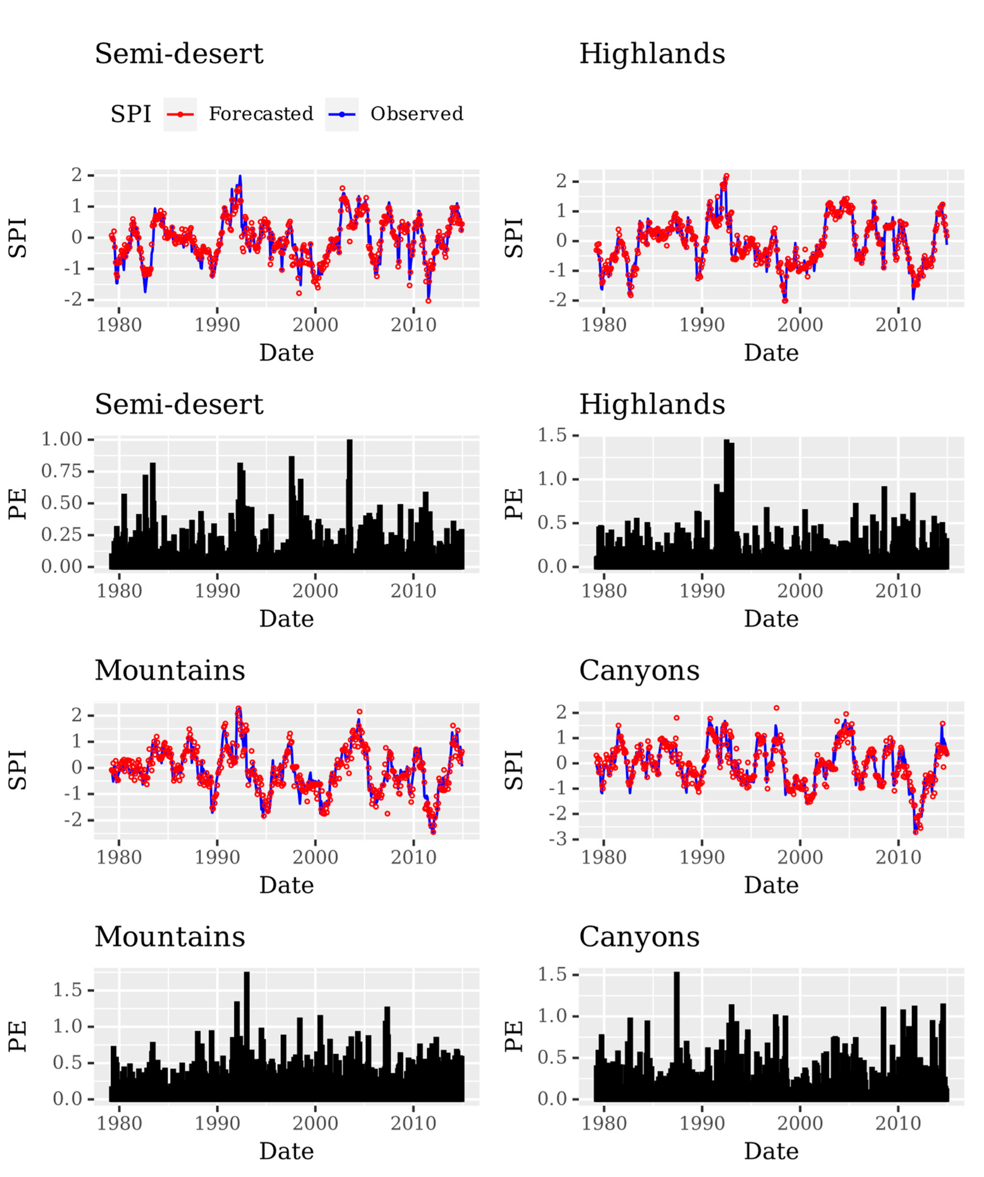
3. Results and Discussion

Results of a neural network with an architecture of 6-25-1 for Semi-desert, Highlands, Mountains and Canyons regions can be observed in Figure 3. In general, training and testing the neural networks using a scaled conjugate gradient as a training algorithm estimated low MSE values and high R values (Table 3). These results suggest that the 4 regional SPI model’s performance was good.
We identified a good correlation (Figure 4) between the observed and predicted values of SPI within the 64-month test period. This result was confirmed by model parameters of linear regression between the observed and predicted SPI values as can be seen in Table 4.
The prediction ability of the NARX models was assessed by analyzing its performance based on the linear regression statistics for all months within the test datasets by means of the R2 and R values (Table 4).
It was evident that the best NARX model predictions correspond to the Semi-desert region. The highest R value (0.9526) belongs to this region. The next best performance was got for the Highlands region next by the Mountains region. Furthermore, the lower R value (0.8443) belongs to the NARX model prediction for the Canyons region. Our results provide convincing evidence of a good SPI prediction ability of the NARX models for all regions in this study.
The probability under normal distribution of the prediction error of the NARX models is summarized in Table 5 and shows the under-predictions (PE < 0) and the over-prediction (PE > 0) skills. An error will be zero when the predicted SPI value exactly matches the SPI observed value [37,38]. Our results indicate that PE < 0 occurrences are higher than PE > 0 occurrences for all but Semi-desert regions. Those results suggest that ANN models under-predicted the SPI for all but the Semi-desert region, where the largest difference found was for the Canyons region with a probability of 58.58% and the smallest difference of 49.65% was found for the Semi-desert region. In addition, the minimum probability value of over-prediction with 41.42% was found for the Canyons region and the maximum probability value of over-prediction error was found for the Semi-desert region with 50.35%. Those results provide support to the ones described by summarized statistics of the linear models between the predicted and the observed SPI values (Table 4).
As mentioned earlier, when analyzing hydrological variables, neural networks have shown their great utility for the empirical prediction of these kind of variables [31,39]. Our results compare well with those of Deo and Şahin [14], Ali et al. [4], Soh et al. [15] and Poornima and Pushpalatha [10], that successfully used other approaches of the artificial neural network model to predict the standardized precipitation index per month.
Furthermore, in good agreement with Liu et al. [34], our study corroborates that the NARX network modeling approach may prove to be successful in formulating the non-linear dynamics in complex systems, particularly as a good tool to forecasting time series. Our results broaden those of Evkaya and Furnaz [40] when forecasting drought by means of NARX because they only use SPI time series and SPI wavelet transformed series and focus on the use of 3-month SPI and 6-month SPI series. Moreover, our findings extend those of Giddings et al. [8] and Magallanes et al. [9] because our approach not only allows defining smaller and detailed regional climatic zones in México by means of the SPI but provides a framework to forecast SPI values.
Most notably, this is the first study to our knowledge to apply NARX models for the prediction of monthly standardized precipitation index with exogenous meteorological inputs. Since the developed NARX models combined the effect of rainfall, temperature, evaporation and evapotranspiration, they have potential to be used as an important tool for water resource assessment. Using the combined influence of these parameters, this could be useful for the detection of climatic and agricultural risks.

4. Conclusions

Lately, the prediction of drought is an important issue for meteorology, hydrology, water resource management and sustainable agriculture because of the vulnerability of human activities relating to water use. We develop nonlinear autoregressive network models with exogenous inputs for predicting the values of four monthly Standardized Precipitation Index (SPI) time series belonging to Mexico’s Zacatecas state territory. The models were trained and tested using the regional monthly time series of rainfall, evaporation, maximum temperature, mean temperature, evapotranspiration and multivariate ENSO index as predictors. The output variable was the forecasted SPI time series for each region.
Based on the results of the evaluation metrics, we have demonstrated that the NARX model is a useful AI tool based on climatological data to forecast the monthly SPI values.
In the matter of climate change, drought forecasting by using NARX models as a framework in future studies would be beneficial for generating useful information for making decisions. In addition, future work should evaluate different ANN models, training algorithms and framework approaches to assess different network architecture effects on model performance.

Author Contributions

Conceptualization, R.M.-Q. and C.E.G.-T.; methodology, R.M.-Q.; software, C.E.G.-T. and J.I.G.-T.; validation, C.E.G.-T. and A.G.-D.; formal analysis, R.M.-Q. and A.G.-D.; investigation, J.I.G.-T. and S.d.J.M.-G.; data curation, R.M.-Q.; writing—original draft preparation, R.M.-Q. and A.G.-D.; writing—review and editing, A.G.-D.; supervision, H.G.-R.; funding acquisition, H.G.-R.; project administration, R.M.-Q. and A.G.-D. All authors have read and agreed to the published version of the manuscript.

Funding

This research received no external funding.

Institutional Review Board Statement

Not applicable.

Informed Consent Statement

Not applicable.

Data Availability Statement

The data used to support the findings of this study is called “Proyecto de bases de datos climatológicos”, was supplied by the “Comisión Nacional del Agua”, the national official institution in charge of climatic and meteorological data record-keeping in Mexico, and is available at: https://drive.google.com/drive/folders/10HCD7X_-sgTIJSQnJE9SkFL92ca3ERDC?usp=sharing (accessed on 30 May 2022).

Conflicts of Interest

The authors declare no conflict of interest.

References

  1. Kharin, V.V.; Zwiers, F.W.; Zhang, X.; Hegerl, G.C. Changes in Temperature and Precipitation Extremes in the IPCC Ensemble of Global Coupled Model Simulations. J. Clim. 2007, 20, 1419–1444. [Google Scholar] [CrossRef] [Green Version]
  2. Angheluţă, P.S.; Badea, C.G. The Water Resources in the Context of Climate Change Produced by the Greenhouse Gases. Ann. Univ. Oradea Fac. Econ. 2015, 1, 637–643. [Google Scholar]
  3. Choubin, B.; Malekian, A.; Gloshan, M. Application of several data-driven techniques to predict a standardized precipitation index. Atmósfera 2016, 29, 121–128. [Google Scholar] [CrossRef] [Green Version]
  4. Ali, Z.; Hussain, I.; Faisal, M.; Nazir, H.M.; Hussain, T.; Shad, M.Y.; Shoukry, A.M.; Gani, S.H. Forecasting Drought Using Multilayer Perceptron Artificial Neural Network Model. Adv. Meteorol. 2017, 2017, 5681308. [Google Scholar] [CrossRef]
  5. McKee, T.B.; Doesken, N.J.; Kleist, J. The relationship of drought frequency and duration to time scales. In Proceedings of the 8th Conference on Applied Climatology, American Meteorological Society, Boston, MA, USA, 17–22 January 1993; pp. 179–183. [Google Scholar]
  6. Naresh Kumar, M.; Murthy, C.S.; Sesha Sai, M.V.R.; Roy, P.S. On the use of Standardized Precipitation Index (SPI) for drought intensity assessment. Meteorol. Appl. 2009, 16, 381–389. [Google Scholar] [CrossRef] [Green Version]
  7. Mahfouz, P.; Mitri, G.; Jazi, M.; Karam, F. Investigating the Temporal Variability of the Standardized Precipitation Index in Lebanon. Climate 2016, 4, 27. [Google Scholar] [CrossRef] [Green Version]
  8. Giddings, L.; Soto, M.; Rutherford, B.; Maarouf, A. Standardized precipitation index zones for Mexico. Atmósfera 2005, 18, 33–56. [Google Scholar]
  9. Magallanes-Quintanar, R.; Blanco-Macías, F.; Galván-Tejada, E.C.; Galván-Tejada, J.I.; Márquez-Madrid, M.; Valdez-Cepeda, R.D. Negative regional Standardized Precipitation Index trends prevail in the Mexico’s state of Zacatecas. Rev. Terra Latinoam. 2019, 37, 487–499. [Google Scholar] [CrossRef] [Green Version]
  10. Poornima, S.; Pushpalatha, M. Drought prediction based on SPI and SPEI with varying timescales using LSTM recurrent neural network. Soft Comput. 2019, 23, 8399–8412. [Google Scholar] [CrossRef]
  11. Ozger, M.; Mishra, A.K.; Singh, V.P. Estimating Palmer Drought Severity Index using a wavelet fuzzy logic model based on meteorological variables. Int. J. Clim. 2010, 31, 2021–2032. [Google Scholar] [CrossRef]
  12. Belayneh, A.; Adamowski, J.; Khalil, B.; Ozga-Zielinski, B. Long-term SPI drought forecasting in the Awash River Basin in Ethiopia using wavelet neural network and wavelet support vector regression models. J. Hydrol. 2014, 508, 418–429. [Google Scholar] [CrossRef]
  13. Masinde, M. Artificial neural networks models for predicting effective drought index: Factoring effects of rainfall variability. Mitig. Adapt. Strat. Glob. Chang. 2013, 19, 1139–1162. [Google Scholar] [CrossRef]
  14. Deo, R.C.; Şahin, M. Application of the Artificial Neural Network model for prediction of monthly Standardized Precipitation and Evapotranspiration Index using hydrometeorological parameters and climate indices in eastern Australia. Atmos. Res. 2015, 161–162, 65–81. [Google Scholar] [CrossRef]
  15. Soh, Y.; Koo, C.; Huang, Y.; Fung, K. Application of artificial intelligence models for the prediction of standardized precipitation evapotranspiration index (SPEI) at Langat River Basin, Malaysia. Comput. Electron. Agric. 2018, 144, 164–173. [Google Scholar] [CrossRef]
  16. Thornthwaite, C.W. An Approach toward a Rational Classification of Climate. Geogr. Rev. 1948, 38, 55–94. [Google Scholar] [CrossRef]
  17. Koudahe, K.; Kayode, A.J.; Samson, A.O.; Adebola, A.A.; Djaman, K. Trend Analysis in Standardized Precipitation Index and Standardized Anomaly Index in the Context of Climate Change in Southern Togo. Atmos. Clim. Sci. 2017, 7, 401–423. [Google Scholar] [CrossRef] [Green Version]
  18. Caloiero, T. Drought analysis in New Zealand using the standardized precipitation index. Environ. Earth Sci. 2017, 76, 569. [Google Scholar] [CrossRef]
  19. Beguería, S.; Vicente-Serrano, S.M. SPEI: Calculation of the Standardized Precipitation-Evapotranspiration Index; R Package Version 1.7; R Foundation for Statistical Computing: Vienna, Austria, 2013. [Google Scholar]
  20. R Core Team. R: A Language and Environment for Statistical Computing; R Foundation for Statistical Computing: Vienna, Austria, 2020. Available online: https://www.cran.r-project.org/ (accessed on 30 May 2022).
  21. Unal, Y.; Kindap, T.; Karaca, M. Redefining the climate zones of Turkey using cluster analysis. Int. J. Clim. 2003, 23, 1045–1055. [Google Scholar] [CrossRef]
  22. Karmalkar, A.V.; Bradley, R.S.; Diaz, H.F. Climate change in Central America and Mexico: Regional climate model validation and climate change projections. Clim. Dyn. 2011, 37, 605–629. [Google Scholar] [CrossRef] [Green Version]
  23. Paradis, E.; Schliep, K. ape 5.0: An environment for modern phylogenetics and evolutionary analyses in R. Bioinformatics 2018, 35, 526–528. [Google Scholar] [CrossRef]
  24. Hanson, R.L. Evapotranspiration and Droughts. In National Water Summary 1988–89: Hydrologic Events and Floods and Droughts; US Geological Survey Water-Supply Paper 2375; US Government Printing Office: Washington, DC, USA, 1991; pp. 99–104. [Google Scholar]
  25. Vicente-Serrano, S.M.; Beguería, S.; López-Moreno, J.I. A multiscalar drought index sensitive to global warming: The standardized precipitation evapotranspiration index. J. Clim. 2010, 23, 1696–1718. [Google Scholar] [CrossRef] [Green Version]
  26. Wolter, K.; Timlin, M.S. El Niño/Southern Oscillation behaviour since 1871 as diagnosed in an extended multivariate ENSO index (MEI.ext). Int. J. Clim. 2011, 31, 1074–1087. [Google Scholar] [CrossRef]
  27. Wolter, K. The Southern Oscillation in surface circulation and climate over the tropical Atlantic, Eastern Pacific, and Indian Oceans as captured by cluster analysis. J. Appl. Meteorol. Climatol. 1987, 26, 540–558. [Google Scholar] [CrossRef] [Green Version]
  28. Wolter, K.; Timlin, M.S. Measuring the strength of ENSO events: How does 1997/98 rank? Weather 1998, 53, 315–324. [Google Scholar] [CrossRef]
  29. Mcculloch, W.S.; Pitts, W.H. A logical calculus of the ideas immanent in nervous activity. Bull. Math. Biophys. 1943, 5, 115–133. [Google Scholar] [CrossRef]
  30. Wang, W.; Van Gelder, P.H.; Vrijling, J.; Ma, J. Forecasting daily streamflow using hybrid ANN models. J. Hydrol. 2006, 324, 383–399. [Google Scholar] [CrossRef]
  31. Farajzadeh, J.; Fard, A.F.; Lotfi, S. Modeling of monthly rainfall and runoff of Urmia lake basin using “feed-forward neural network” and “time series analysis” model. Water Resour. Ind. 2014, 7–8, 38–48. [Google Scholar] [CrossRef] [Green Version]
  32. Carbonera, L.F.B.; Bernardon, D.P.; Karnikowski, D.D.C.; Farret, F.A. The nonlinear autoregressive network with exogenous inputs (NARX) neural network to damp power system oscillations. Int. Trans. Electr. Energy Syst. 2020, 31, e12538. [Google Scholar] [CrossRef]
  33. Diaconescu, E. The use of NARX neural networks to predict chaotic time series. WSEAS Trans. Comput. Res. 2008, 3, 182–191. [Google Scholar]
  34. Liu, Q.; Chen, W.; Hu, H.; Zhu, Q.; Xie, Z. An Optimal NARX Neural Network Identification Model for a Magnetorheological Damper with Force-Distortion Behavior. Front. Mater. 2020, 7, 10. [Google Scholar] [CrossRef]
  35. The Mathworks. MATLAB. 2021. 9.7.0.1190202 (R2021b); The MathWorks Inc.: Natick, MA, USA, 2021. [Google Scholar]
  36. Chapra, S.C.; Canale, R.P. Numerical Methods for Engineers; McGraw-Hill Higher Education: Boston, MA, USA, 2006. [Google Scholar]
  37. Moustris, K.P.; Ziomas, I.C.; Paliatsos, A.G. 3-Day-Ahead Forecasting of Regional Pollution Index for the Pollutants NO2, CO, SO2, and O3 Using Artificial Neural Networks in Athens, Greece. Water Air Soil Pollut. 2009, 209, 29–43. [Google Scholar] [CrossRef]
  38. Moustris, K.P.; Larissi, I.K.; Nastos, P.T.; Paliatsos, A.G. Precipitation Forecast Using Artificial Neural Networks in Specific Regions of Greece. Water Resour. Manag. 2011, 25, 1979–1993. [Google Scholar] [CrossRef]
  39. Daliakopoulos, I.N.; Coulibaly, P.; Tsanis, I.K. Groundwater level forecasting using artificial neural networks. J. Hydrol. 2005, 309, 229–240. [Google Scholar] [CrossRef]
  40. Evkaya, O.O.; Kurnaz, F.S. Forecasting drought using neural network approaches with transformed time series data. J. Appl. Stat. 2020, 48, 2591–2606. [Google Scholar] [CrossRef] [PubMed]
Figure 1. Study region of Zacatecas state within the Mexican territory.
Atmosphere 13 01254 g001
Figure 2. NARX neural network structure.
Atmosphere 13 01254 g002
Figure 3. The observed, forecasted and absolute prediction error for regional SPI time series for the Zacatecas state territory.
Atmosphere 13 01254 g003
Figure 4. Correlation and trend lines between the original SPI values and the forecasted NARX SPI values in test period for regional SPI time series for Zacatecas State, Mexico.
Atmosphere 13 01254 g004
Table 1. Classification of standardized precipitation index values.
SPI ValueClass
≥2.0Extremely wet
1.5 to 1.99Severely wet
1.0 to 1.49Moderately wet
−0.99 to 0.99Near normal
−1.49 to −0.99Moderately dry
−1.99 to −1.49Severely dry
≤2.0Extremely dry
Table 2. Summary of input predictors by region used in the ANN models.
Region
Semi-AridSPIPP (mm)EVP (mm)TMED (°C)TMAX (°C)PET (mm)
Min−1.95770.000079.929710.175321.780724.6523
µ−0.068534.2184163.986316.795329.389065.0969
Max1.9913282.3329304.652522.445237.0236116.3594
σ0.695038.230647.10193.11632.666023.8464
HighlandsSPIPP (mm)EVP (mm)TMED (°C)TMAX (°C)PET (mm)
Min−1.98030.000083.382010.144122.507020.2253
µ−0.067137.2929172.048416.785129.417869.3710
Max2.0847263.7820311.162125.270036.0990121.6185
σ0.772942.796751.09853.24872.751227.0455
MountainsSPIPP (mm)EVP (mm)TMED (°C)TMAX (°C)PET (mm)
Min−2.49410.000066.716712.066718.662324.7254
µ−0.090350.3055172.184219.779332.772367.3928
Max2.2986294.1333338.066726.533339.5000271.1664
σ0.840158.906657.14133.50753.127727.3713
CanyonsSPIPP (mm)EVP (mm)TMED (°C)TMAX (°C)PET (mm)
Min−2.75630.000072.550910.120024.875020.2253
µ−0.044962.5014153.508818.884231.683769.3710
Max1.7283350.5735654.138924.825038.3750121.6185
σ0.836176.366757.75393.23122.808327.0455
Table 3. Quantitative measures of the ANN performance in training and test phases for regional SPI time series for Zacatecas State, Mexico. Key measures: Mean Square Error (MSE) and Correlation coefficient (R).
RegionMSER
Semi-desert
Training0.08130.9099
Test0.11970.8936
Highlands
Training0.08260.9341
Test0.04860.9631
Mountains
Training0.08890.9365
Test0.08140.9514
Canyons
Training0.07590.9426
Test0.09910.9399
Table 4. ANN models’ performance using linear regression models (SPIp = β0 + β1 SPIo) of observed SPI values (SPIo) and the forecasted SPI values (SPIp) within test period for regional SPI time series for Zacatecas State, Mexico.
Regionβ0β1R2R
Semi-desert−0.00990.84280.90760.9526
Highlands0.02920.94170.79740.8930
Mountains−0.031580.90440.77670.8813
Canyons0.05950.87380.71280.8443
Table 5. The probability under normal distribution of prediction error (PE) for observed SPI values (SPIo) and the forecasted SPI values (SPIp) in test period for regional SPI time series for the state of Zacatecas, Mexico.
RegionPE < 0PE > 0
Semi-desert0.49650.5035
Highlands0.50580.4942
Mountains0.51750.4825
Canyons0.58580.4142
Publisher’s Note: MDPI stays neutral with regard to jurisdictional claims in published maps and institutional affiliations.

