Article

Understanding the El Niño Southern Oscillation Effect on Cut-Off Lows as Simulated in Forced SST and Fully Coupled Experiments

1
Department of Atmospheric Sciences, University of Sao Paulo, Sao Paulo 05508090, Brazil
2
Department of Meteorology, The University of Reading, Reading RG6 6AH, UK
3
Center for Weather Forecast and Climate Studies (CPTEC), National Institute for Space Research (INPE), Sao Jose dos Campos 12227010, Brazil
*
Author to whom correspondence should be addressed.
Atmosphere 2022, 13(8), 1167; https://doi.org/10.3390/atmos13081167
Submission received: 2 June 2022 / Revised: 20 July 2022 / Accepted: 21 July 2022 / Published: 23 July 2022
(This article belongs to the Special Issue Coupled Climate System Modeling)

Abstract

:
In this study, we show that changes in the 250 hPa vorticity cut-off low (COL) activity may possibly be driven by sea surface temperature (SST) variations in the tropical Pacific. Using ERA5 reanalysis, the existence of different large-scale circulation patterns is identified that work to enhance the COL activity with a weakened jet stream, while COLs are suppressed with strengthened westerlies. The present-day simulations of AMIP-CMIP6 models reproduce realistic features of the El Niño Southern Oscillation (ENSO)–COL teleconnection, but biases exist, especially in coupled models. The differences are a priori due to the inability of the models to accurately predict the time-mean zonal flow, which may be in part due to systematic biases in the predicted SST. The underestimation of warm SST anomalies over the eastern Pacific is a common problem in CMIP3 and CMIP5 models and remains a major uncertainty in CMIP6. We find that a reduced bias in the predicted SST by coupled models is most likely to produce more skillful simulations in the Southern Hemisphere, but the same evidence does not hold for the Northern Hemisphere. The study suggests the potential for seasonal prediction of COLs and the benefits that would result using accurate initialization and consistent model coupling.

1. Introduction

Cut-off low (COL) systems are synoptic-scale features characterized by a mid-upper-tropospheric cold low (depression) that has become completely detached from the main westerly flow. COLs have important implications for the local weather as they are typically associated with high rainfall and flooding in midlatitude and subtropical regions and also impact ozone concentrations due to stratosphere-troposphere exchange. Because of the importance of COLs in affecting the weather, understanding the characteristics of COLs and their variability is of particular interest for numerical weather and climate predictions. Many observational and numerical studies have investigated COLs from different perspectives [1,2,3,4,5,6]. Despite the recent advances in our understanding of COLs, the influence of teleconnection patterns on COLs and their predictability have received much less attention.
Given that El Niño Southern Oscillation (ENSO) is the dominant mode of interannual variability in the tropics and has significant impacts on the global climate, there is interest in how COLs might respond to changes in the tropical Pacific sea surface temperature (SST). There are compelling reasons to assume that the tropics might have a relevant influence on the COL activity. Many studies have shown that El Niño (La Niña) events can modify the Hadley circulation [7,8,9], affecting the subtropical eddy momentum flux and possibly the behavior of stationary or quasi-stationary systems such as blocking and COLs. Blocking and COLs are found to be strongly associated [10], and both are generally related to zonally weakened upper-level jets, which are commonly manifested as a split jet [11]. The effect of ENSO patterns on jet strength and zonality has been studied widely and may also be a key component in explaining variations in the COL activity.
ENSO impacts have primarily been investigated in terms of particular COL statistics, especially the number of COLs, but also their location, which can be derived from the tracks of COLs, which in turn can provide additional information such as velocity, length, and lifetime. For the southern African region, [12] observed that La Niña events are associated with an above-average number of COLs, though the opposite does not necessarily hold for El Niño years. The ENSO variability affects the jet structure and modifies the COL occurrence by shifting the jet equatorward of its climatological position during La Niña and poleward during El Niño, implying that COLs are more numerous at lower latitudes during La Niña and at higher latitudes during El Niño [13]. Although these previous studies provide an insight into the relationship between ENSO phases and COL activity, statistically significant correlations have not been observed in all studies in both hemispheres, as discussed in [14] and [15]. Contradictions in the findings concerning the COL statistics and the lack of a statistical difference in their activity between ENSO phases highlight that the link between ENSO and COLs is still not entirely understood. Therefore, further research is needed in order to obtain more robust conclusions about the effect of the Pacific SSTs on COL occurrence. In addition, the accurate COL response to oceanic forcing by climate models would be of great interest for the seasonal prediction of COL activity, especially because there is little published work on this topic.
In recent years, several studies have been performed to simulate ENSO features and associated teleconnections using coupled general circulation models (GCMs) [16,17,18,19,20]. The advances in available computing sources have allowed the use of coupled GCMs with high enough resolution to study the atmospheric circulation and their response to oceanic conditions. The recent study by [21] provides a robust assessment of phases 5 and 6 of the Coupled Model Intercomparison Project (CMIP) in simulating the climatological aspects of COLs. Using fully coupled models, [21] found improvements in the representation of location and intensity of COLs in CMIP phase 6 (hereafter CMIP6) compared to those in CMIP5, which is mainly attributed to finer spatial resolution models and improved model parameterizations and physical processes. Since GCMs can provide useful information to detect a possible link between the interannual variability of COLs and SST anomaly changes, the study reported here extends the [21] study to how climate models simulate the ENSO effects on COLs regionally.
Given that the response of COLs to Pacific SSTs continues to be limited to specific regions, and considering that the underlying physical mechanisms are still unclear, it is important to determine whether and how the ENSO affects the COL activity in both hemispheres using a more modern reanalysis product (i.e., ERA5) than those used in earlier studies. In addition, this study aims to investigate how the COL response to ENSO is simulated by the state-of-the-art CMIP6 models. Here, the coupled model simulations are assessed together with the corresponding Atmospheric Model Intercomparison Project phase 6 (AMIP6) runs. This helps to understand the differences between coupled and uncoupled atmosphere-only simulations and to document potential errors in the air-sea interaction. The AMIP6 simulations are forced by observed SSTs and sea ice concentration and do not include coupled ocean-atmosphere interactions [22], while the CMIP6 models have a fully dynamical and interactive ocean; therefore, it is important to assess the performance of the two experiments in simulating COLs and their response to ENSO. The aim of the paper is two-fold. The first is to examine how ENSO conditions affect COLs in each hemisphere. The second is to contrast the differences between AMIP6 and CMIP6 simulations and determine which of the two experiments produces a more realistic atmospheric response. Both AMIP6 and CMIP6 are used as there is interest in documenting possible errors in the coupled model predicted SSTs and their effect on the representation of COLs and how the results compare with simulations forced with observed SSTs.
The paper is organized as follows. Section 2 provides a brief description of the reanalysis data, models, and analysis methods used. Section 3 discusses the impact of ENSO on COLs observed in the ERA5 reanalysis and simulated in coupled and uncoupled models. Summary and conclusions are given in Section 4.

2. Data and Analysis Procedures

The study examines the COL response to ENSO using data from AMIP6 and CMIP6 simulations. The same set of models is used for both experiments, as listed in Table 1. The period used for the analysis is the historical period 1979–2014, and models were chosen based on their availability for the study, with all available ensemble members being used to reduce the uncertainty in the analysis. COLs identified in the European Centre for Medium-Range Weather Forecasts (ECMWF) fifth generation reanalysis (ERA5) are used to validate the models for the period 1979–2014. ERA5 is the most recent reanalysis data set produced by ECMWF, available at a horizontal resolution of 31 km with 139 vertical levels [23], which is a much higher resolution than the older ERA-Interim reanalysis, which is approximately 80 km [24].
To track the COLs in the reanalysis and model data, the TRACK algorithm [25,26,27] is used with a specific COL detection scheme [28]. The tracking is first performed to track all systems using 6-hourly relative vorticity at 250 hPa ( ξ 250 ), then a COL detection scheme is applied to the zonal and meridional wind components in four offset points around the tracked vortex center to restrict the identification only to closed depressions, as detailed in [28]. Spatial statistics are produced from the tracks using spherical kernel estimators [26] for track and genesis densities. The diagnostics described here have been performed for both hemispheres for all four seasons, but only the mean fields averaged over all seasons are shown for reasons of simplicity and convenience. COL track density anomalies are computed by subtracting the climatology from the El Niño and La Niña statistics in each model and the reanalysis. ENSO events are defined using the normalized monthly SST anomalies (averaged over a season for the spatial statistics) in the Niño-3.4 region (5° S–5° N and 120°–170° W) greater than +1.0 °C (El Niño) and less than −1.0 °C (La Niña) based on the National Oceanic and Atmospheric Administration (NOAA) Oceanic Niño Index (ONI) from the reconstructed SST version 3b (ERSST.v3b). Using a moderate Niño-3.4 SST anomaly as a criterion for defining cold/warm events might produce an enhanced response to the COL activity. This is done for the ERA5 and AMIP6 data, whereas for CMIP6, the Niño-3.4 is produced using the model predicted SST for each model and each ensemble member as they will generate their own ENSO cycles different from observations.
To test whether the variations in the COL activity are correlated with ENSO and if the correlations are statistically significant, the Pearson’s correlation coefficient between monthly COL counts and ENSO is computed together with a two-sample Student’s t-test. The time-lagged correlation coefficients are also calculated on the two time series. In addition, wavelet analysis is applied to provide a qualitative measure of changes in COL variance to ENSO on interannual to decadal time scales. The wavelet transform is a powerful tool for analyzing dominant modes of variability, and numerous studies have been conducted using wavelets to identify the fluctuations in ENSO variance and its different interactions and feedback processes [29,30,31,32,33]. The cross-wavelet spectrum is the technique used here to investigate the relationship between ENSO phases and COL counts as the wavelet coherency is more complex and dependent on an arbitrary smoothing function [29].

3. Results

We begin by presenting the COL relationship to ENSO observed in ERA5. The link between COLs and the ENSO phases is investigated using counts and spatial statistics. Later, we evaluate the predictability of the AMIP6 and CMIP6 models in simulating COLs in both hemispheres and discuss potential relationships to the corresponding upper-level zonal flow and SST bias.

3.1. ERA5

3.1.1. Northern Hemisphere

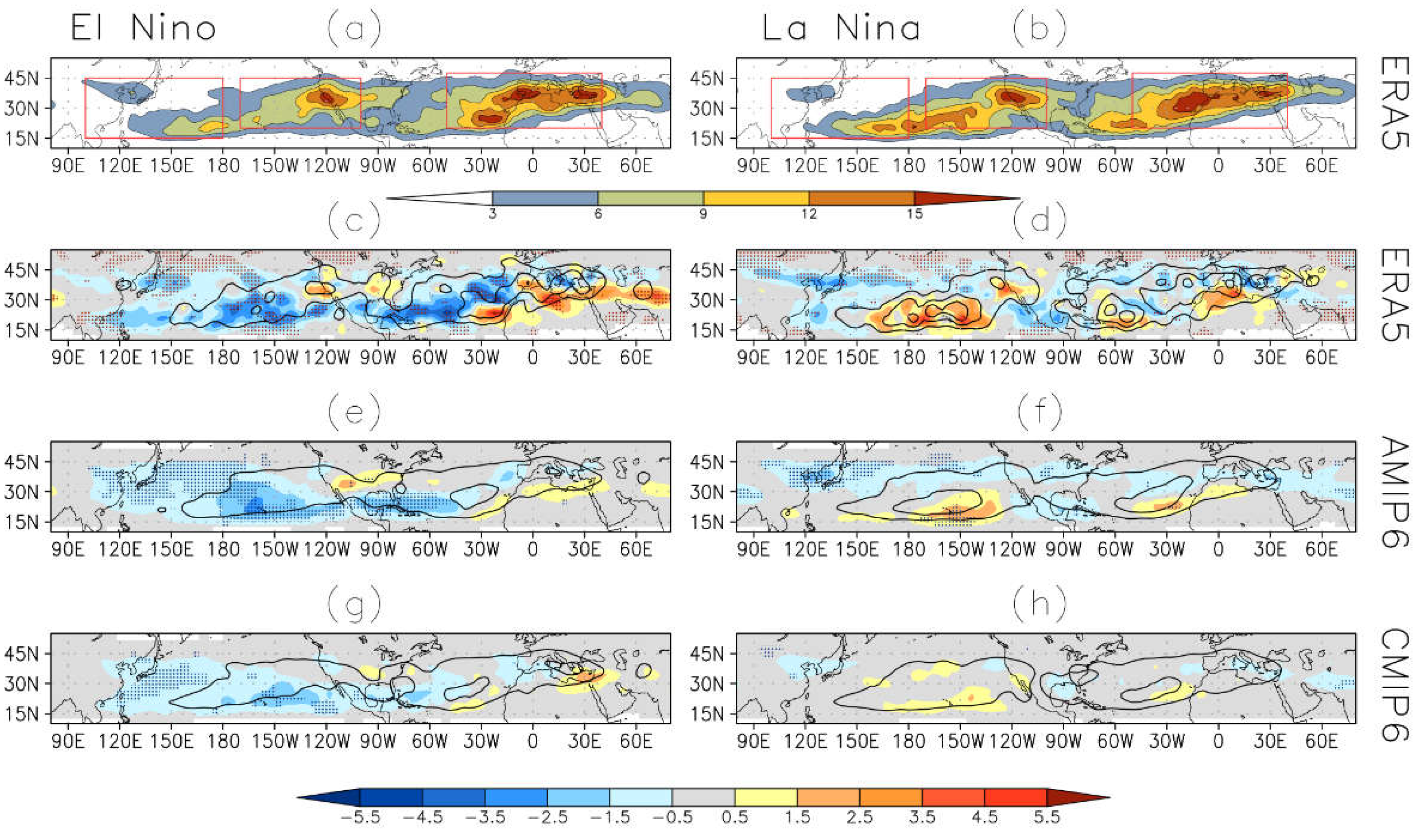
Since the climatological locations of COLs in the Northern Hemisphere have been extensively discussed in the literature [34,35,36,37], it is of interest here to focus on the response of COLs to the ENSO phases. The COL track density for El Niño and La Niña years for the period 1979–2020 are shown in Figure 1a,b, respectively, only to provide information on the general distribution of COLs. Figure 1c,d show the track density anomaly of COLs calculated as El Niño and La Niña composites minus the climatology (shaded) combined with the genesis density (contour) for each ENSO phase averaged over all seasons for ERA5. The tracking is performed separately for each season, but only the averaged fields are shown for reasons of simplicity (see Figure S1 in the Supplementary Material for detailed seasonal analysis). In the El Niño composite, there is a significantly reduced track density across almost the whole North Pacific, which are significant at a confidence level of 90% by the Student t-test (cross-hatching). In contrast, the La Niña composite shows an overall increase with a southward shift of COL tracks over the North Pacific, though most of the positive anomalies are not statistically significant. Some studies have used different field significance tests based on Monte Carlo methods [38,39] to provide a measure of global significance that requires much additional computation, and it is not clear what the best approach is for the type of data used in the study.
A closer inspection of individual ENSO events reveals they have different amplitude and spatial distribution (not shown). During the La Niña event of 1984–1985, in particular, the negative SSTs were mostly confined in the eastern tropical Pacific, which is a more common feature in the Niño-3 region, while the central Pacific, previously referred to as Niño-3.4, presented small negative SST [40]. The spatial pattern characterized by intensified cold SST anomalies in the eastern Pacific seems to induce a strong atmospheric response near the west coast of North America rather than the central Pacific, thus resulting in more COLs in the northeastern Pacific (not shown). The results suggest that the spatial distribution of SST anomalies may play a role in determining the region where the COL activity is changed.
In North America, there appears to be no obvious difference in the track density during ENSO periods, as indicated by the lack of significance, but again the results may be sensitive to the statistical significance method. The exception is seen in south Texas and northeast Mexico, which exhibit statistically significant decreasing densities in El Niño. A notable increase in track density is observed in western North America in both ENSO phases and during all seasons (see Figure S1 as Supplementary Material), but this change is significant only at 80% (not shown). Although our composites based on warm and cold ENSO events show little statistically significant anomaly over the United States, other studies suggest the existence of statistical linkages between ENSO state and seasonal precipitation anomalies in North America [41,42]. One possibility is that the sign of precipitation found in other studies may not be due to COL-associated precipitation but to other systems that we have not looked at here. Although neutral ENSO conditions account for two-thirds of the total period, the highest number of tracks in western North America occurred during warm and cold ENSO episodes (autumn 1987 and summer 1988). It is not clear what could be producing such an anomaly in COL track density in western North America, and other North Pacific variability modes may be affecting COL activity, such as the Pacific-North American (PNA) and the Pacific Decadal Oscillation (PDO). Investigating each of these possible teleconnection linkages is beyond the scope of the study but should be taken into consideration in further research.
The response of COL activity to ENSO in the North Atlantic is somewhat similar to that observed in the North Pacific as a clear decrease in track density occurs during El Niño, though an increase can be seen off the coast of northwest Africa near the western Sahara and Mauritania. Our findings confirm previous research that the warm phase of ENSO is associated with an increase in the occurrence of COLs in the Iberian Peninsula, Northern Africa, and the Middle East [11,43]. During La Niña episodes, the COL activity is enhanced at lower latitudes in the North Atlantic, but the changes are less pronounced compared to those observed in the North Pacific. Despite the evidence supporting the relevance of ENSO to the North Atlantic and European COLs, the monthly time series reveals there are frequently opposite impacts on the frequency of tracks from year to year under the same ENSO phase, which suggests that considering other teleconnection patterns occurring in the North Atlantic area, e.g., North Atlantic Oscillation [11], is a key in understanding the interannual variability of COLs.
The time-lagged Pearson cross-correlation and wavelet analysis are applied to investigate the relationship between the time series of monthly COL numbers and the Niño-3.4 index for the period 1979–2020. Wavelet analysis is useful to detect when variability becomes significant during particular periods, and in the present study, the cross-wavelet transform with a 95% confidence level is applied to investigate the dominance of signals for three preferred locations of COLs in each hemisphere, shown in Figure 2. These regions are similar to those described in earlier studies [15,36], except for the Asian sector, which covers more southern latitudes than previously considered. In earlier studies, systems between 20° S and 20° N were excluded, but we consider it important to extend the domains to lower latitudes to adequately sample as many COLs as possible.
For the European sector, the cross-wavelet power (Figure 2a) indicates large covariance between ENSO and COL number at scales of approximately 24–48 months during 1984–1992, 1993–2002, and 2007–2020. The phase difference (indicated by the vector angular orientation) varies smoothly near the 24–48 months band and indicates a positive lag relationship between COL number and ENSO. This means that changes in COL counts lead the Niño-3.4 index by a month or so. The analysis of time-lagged correlations explored for a range of time lags confirms that there is a statistically significant positive one-month lag correlation for Europe during spring. The mechanisms underlying the observed findings are unclear, but we suggest that fluctuations in COL activity may not be directly forced by the SST anomalies in the Niño-3.4 region. The time delay among the time series may result from air-sea interaction associated with the evolution of SST anomalies outside the Niño-3.4 region, such as in the western Pacific [44] and Indian Ocean [45]. These mechanisms need to be further investigated with focused studies.
The cross-wavelet power for North America (Figure 2b) demonstrates an annual cycle that is observed at regular intervals of approximately 12 months, though they are not persistent over time. There is also an ENSO signature with phase difference approximately constant in the 20–48 months signals during 1983–1990 and the 28–34 months during 1994–1997. The cross-lagged correlation suggests the existence of a seasonally dependent relationship between COL number in North America and the Niño-3.4 index, with the predominance of positive correlations during summer–autumn and negative correlations during winter–spring. The apparent seasonal cycle in ENSO and its effect on the COL activity is shown in [15], and possible reasons for ENSO’s irregularity in impacting COLs are discussed in several studies [46,47,48,49]. The cross-wavelet power spectrum for Asia (Figure 2c) is similar to that for North America, though signals are more uniformly distributed over time. Nevertheless, there is relatively low variability for time periods longer than one year, suggesting the influence of ENSO on Asian COLs is less clear than in other sectors.
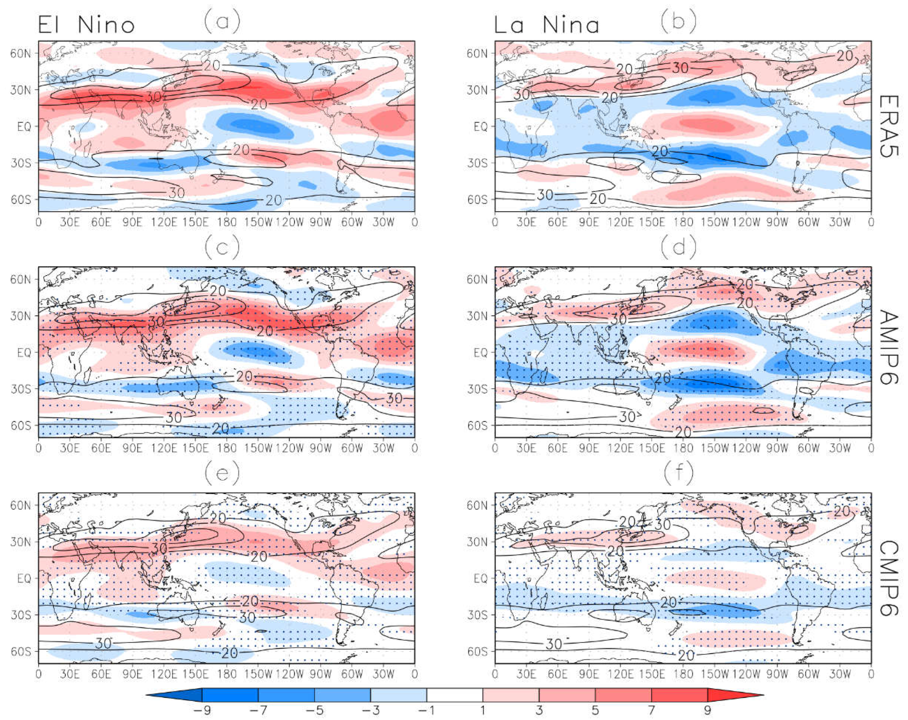
After demonstrating the role of tropical Pacific SSTs on the spatial and temporal variability of COLs, the investigation of the large-scale circulation is further extended to understand the response of COL activity to the changes in the zonal mean flow in each ENSO phase. The zonal circulation in the upper troposphere has been used as a measure of uncertainty in the simulation of COLs [21], and many studies have shown that changes in the zonal wind spatial distribution and strength on interannual time scales are strongly related to ENSO [50,51,52,53]. The 250 hPa zonal wind ( U 250 ) anomaly in ERA5 (Figure 3a,b) shows that the Northern Hemisphere jet stream is greatly enhanced and located southward to its climatological position during the warm phase of ENSO. The anomalous westerlies are associated with the strengthening and contraction of the Hadley cell [54,55]. The observed changes in COL activity may occur as a consequence of the equatorward displacement of the westerlies during El Niño, which is likely responsible for the reduced densities over the North Pacific, southern United States, and North Atlantic, as discussed above. On the other hand, the equatorward shift in the mean position of the jet stream over the European-Asian region reduces the velocity north of the jet entrance region, which may be related to the increased activity of COLs in the Iberian Peninsula and north Africa. The most significant differences observed between ENSO phases occur in the central-eastern Pacific Ocean, where upper-level winds exhibit a dipole-like mode between tropics and extratropics (Figure 3a,b). Overall, we find that the COL track density anomaly is negatively correlated (although weak) with the U 250 anomaly, i.e., the COL activity tends to enhance (suppress) under reduced (increased) zonal winds. The negative correlation coefficients were identified in all seasons and reached −0.4 during boreal winter for La Niña. The weak correlation might be caused by the nonhomogeneous correlation between track density and U 250 as the COL activity tends to enhance equatorward from the region where the westerlies are weakened. This is a consequence of the wave-breaking phenomenon and is clearly seen from the seasonal fields available in the Supplementary Material (Figure S3). This result reinforces the idea that the subtropical jet controls the position of COLs since the zonal mean background flow associated with El Niño (La Niña) induces a higher frequency of weak (strong) wave-breaking events on the equatorward side of the eddy-driven jet [56].

3.1.2. Southern Hemisphere

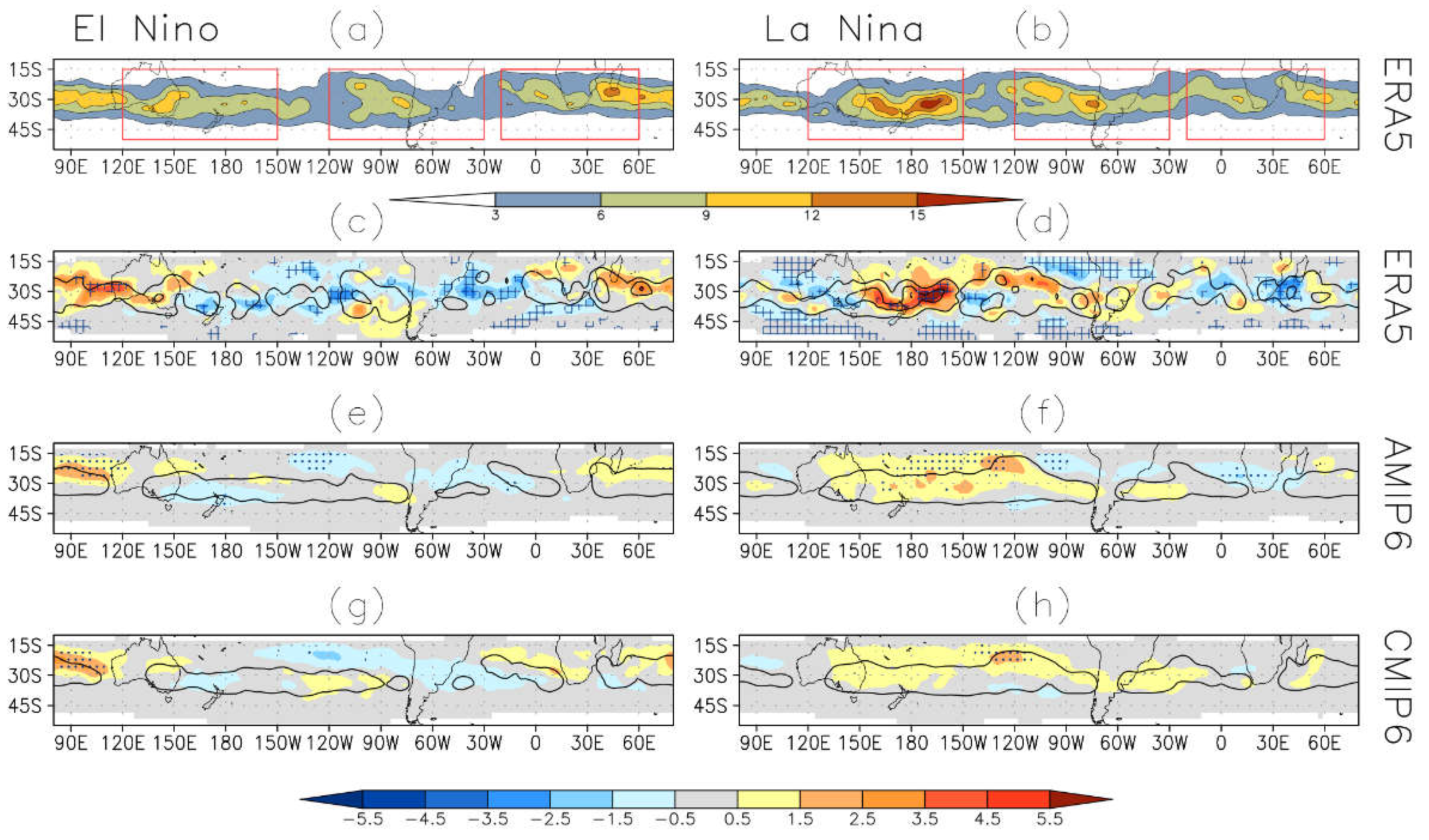
There are some differences in changes in COL location in the Southern Hemisphere (Figure 4a,b) from those observed in the Northern Hemisphere (Figure 1a,b). The differences may be attributed to the differences in land-sea contrast and topography between the two hemispheres, which influence the nature and propagation characteristics of (stationary) Rossby waves and consequently impact COLs. During El Niño, the genesis and track densities of COLs (Figure 4c) are anomalously enhanced across the Indian Ocean and Australia, which is statistically significant at a 90% confidence level, representing an increase of 25% compared to climatology. In addition, the El Niño composite exhibits positive track density anomalies from the southeast Pacific into high latitudes of South America, but they are significant only at 80% (not shown) for the significance test used here. This result is consistent with the increased number of blocking events over the southeast Pacific during El Niño years [57], as COLs and blocking are commonly considered the same phenomenon, differing only in the upper-level potential vorticity anomalies [58]. A reduction in track density occurs in other areas of the South Pacific, subtropical South America, and South Atlantic.
The La Niña composite (Figure 4d) shows nearly opposite patterns to that observed in the El Niño composite. The highest COL activity shifts to the east, and the regions with maximum COL genesis appear in southeast Australia, north of New Zealand, and southwestern Pacific. The La Niña periods are also associated with higher COL densities in Northern Chile and favored conditions for the formation of COLs off the coast of the Atacama Desert. The connection between ENSO and COLs in the African sector discussed in earlier studies [12,13] is demonstrated in our analysis, confirming that COLs are more frequent over the western coast of southern Africa during La Niña and over the eastern coast during El Niño [13]. Nonetheless, there is not a clear latitudinal displacement of COLs during ENSO phases, contradicting earlier findings by [13], which found an equatorward shift of COLs during La Niña. These differences may be due to different methods and reanalysis data sets, as previously discussed [28,59].
Considering the whole Southern Hemisphere, there is a statistically significant decrease in the average number of COLs during El Niño years (~10% below average, p-value < 0.05), but no significant changes are observed in La Niña years, though there are large seasonal differences (see Figure S2 in the Supplementary Material) and frequently opposite effects between regions that appear to affect more often the COLs in the Southern Hemisphere than those in the NH (Table 2). The relationship between COLs in the Australian region and the Niño-3.4 index is shown in Figure 2d. The cross-wavelet power indicates large covariance between time series at scales of 10–16 months. There is high power associated with signals on the 32–48 months timescales at the beginning and end of the period, but they are mostly outside the region of significance (cross-hatched region), and thus it is unclear whether the peaks in this region are a true variance or an artifact of the padding [60]. We can see signals at very long (decadal) length periods in the whole cross-wavelet power spectrum, though these are not statistically significant at a 95% confidence level. The cross-wavelet spectrum for South America (Figure 2e) shows that the power is broadly distributed with peaks in the 12–56 months ENSO band. It can be seen a power peak significant at >95% confidence level in the 16–32 months periodicity during 1994–2000 (encompassing the strong 1998–2000 La Niña), which are approximately 180° out of phase, indicating an association between the increased number of COLs in South America and La Niña. The cross-wavelet spectrum for Africa (Figure 2f) reveals that the power is broadly distributed with peaks in the 10–24 months band. The 95% confidence level regions demonstrate common features associated with ENSO variance in the 44–56 months periods during 1986–1991 and the 32–44 months during 2012–2018. These phase relations in the African region show a clear positive time lag between ENSO and COL numbers, indicating that SST leads the COL variation.
We further apply an analogous analysis to the Northern Hemisphere to understand how the circulation changes with ENSO influence the COL distribution in the Southern Hemisphere. It can be seen from Figure 3a that the upper-level westerlies are enhanced across the subtropical central-southeastern Pacific during El Niño, and this pattern seems to act to suppress COL activity. The opposite holds for La Niña (Figure 3b) when weakened westerlies extending from eastern Australia and the South Pacific create conditions for wave breaking and COL formation. A similar effect occurs in the South Indian Ocean during El Niño when weaker zonal winds favor an increase in the number of COLs. The spatial correlations between U 250 and track density anomalies over austral latitudes were found to be negative for both El Niño ( ρ = −0.37) and La Niña ( ρ = −0.34), reinforcing the link between COLs and upper-level jet streams. This result supports earlier conjectures that the mean zonal wind deceleration in the upper troposphere offers conditions for Rossby wave breaking and COL development [2].

3.2. CMIP6 Models

3.2.1. Global SST Bias

Given that SSTs are one of the key parameters for accurate climate predictions, we first analyze how the spatial distribution of SST is simulated in the CMIP6 models, particularly in the tropical Pacific Ocean. Figure 5b shows the time-mean bias in the SST prediction for the ensemble of CMIP6 models, obtained from the difference in the mean SST of the ensemble-averaged coupled model and ERA5 reanalysis. A common feature of the models is their pronounced SST bias in the upwelling zones over the regions off the west coast of Africa and South America that exceeds 2.0 °C, associated with a cloud-related shortwave radiative bias, according to [61,62,63]. Positive systematic biases are also particularly visible at mid-high latitudes in the Southern Hemisphere, while negative biases are seen in the North Pacific and North Atlantic (subarctic regions). Despite the uncertainties regarding the model data, the SST bias in the central tropical Pacific is substantially reduced in CMIP6 compared to CMIP3 and CMIP5 [64,65], apparently associated with a reduced cold tongue bias relative to previous model versions.
We further show the interannual variance of SST as the focus of our analysis is on the ENSO-related interannual variability. The spatial distribution of SST variance observed in the reanalysis (Figure 5a, aqua color) and simulated by the multi-model ensemble mean (Figure 5b) are similar, though the model generally underestimates the variance seen in the ERA5 results, as observed in the tropical eastern Pacific and along the west coast of South America. This is likely a consequence of the warm bias of SST in the eastern Pacific related to misrepresentation of the SST cooling resulting from errors in the dynamical forcing of the ocean within the coupled systems [66].
Figure 5c,d provide the spatial pattern of composite SST anomalies during the warm and cold phases of ENSO simulated by the ensemble mean of CMIP6 models. The analysis shows a similar spatial pattern between El Niño and La Niña, where the stronger SST anomalies are located over the central Pacific (100°–80° W) with maximum values of approximately 1.5–2.5 °C in both ENSO phases. In general, the simulated cold SST anomalies along the equator are closer to the reanalysis, whereas the maximum warm SST anomalies are positioned too far to the west, characterizing an unrealistic weak El Niño–La Niña asymmetry. As previously observed, the major cause for the weak ENSO asymmetry in the CMIP6 models is the underestimation of the warm SST anomalies over the far eastern Pacific during El Niño, particularly in the coastal regions [67]. This is a systematic bias present in CMIP6 models [68] and a common problem in CMIP3 and CMIP5 models [65,69]. The underestimation of the ENSO asymmetry is specifically attributed to the inability of models to properly simulate the ENSO nonlinearity [70,71,72]. A quantitative analysis reveals that all the CMIP6 models underestimate the observed warm SST anomalies over the tropical Pacific (exceptions are MIROC6 and MIROC-ES2L), which is more severe in the eastern Pacific. Although more serious bias arises during the warm phase, coupled models are locally and globally better correlated with ERA5 in El Niño ( ρ   = 0.89) than in La Niña ( ρ   = 0.83). Given the problems described above, an important question from this study is how the model systematic errors in SST will affect the atmospheric circulation and, consequently, the COL activity. This will be discussed further below.

3.2.2. Northern Hemisphere

Our aim in this section is to assess the skill of the multi-model ensemble of AMIP6 and CMIP6 simulations in reproducing the main features of the observed COLs in response to ENSO. Following [21], the spatial statistics are produced from the ensemble mean of each model, which is used to compute the multi-model ensemble mean, then models with a different number of members contribute equally to the eight-model ensemble mean. This is helpful in dealing with prediction uncertainty that usually arises from a single forecast. Systematic bias is defined as common errors either when all models have a bias with positive or negative signs, denoted by stippling.
The track density anomalies and genesis density obtained from the multi-model ensemble mean of AMIP6 (CMIP6) are shown in Figure 1e,f (Figure 1g,h) for El Niño and La Niña periods, respectively. During El Niño, the decrease in COL activity in the North Pacific and North Atlantic oceans seems to be reasonably well reproduced by both AMIP6 and CMIP6, which is a common feature in all simulations (indicated by the stippling), particularly from atmosphere-only models, although this reduction is smaller than that observed in ERA5. The increase in COL activity in the North Pacific associated with the equatorward shift of COL tracks during La Niña is also accurately predicted by AMIP6, but the response is too weak in CMIP6. Similarly, during the La Niña phase, the CMIP6 models exhibit too weak anomalies in the North Atlantic. This appears to be related to a difficulty that the coupled models have in reproducing the COL features during La Niña conditions. The COL location changes observed over southern Europe/North Africa in ERA5 appear rather weak or even negligible in the simulations, and this seems to be a cause of the difference between models so that there is much cancellation between positive and negative values. The correlation coefficients of the simulated and observed spatial distribution of track density indicate comparable predictive skill between AMIP6 ( ρ   = 0.69) and CMIP6 ( ρ   = 0.60) simulations during El Niño, but reduced correlations occur during La Niña conditions with ρ   = 0.53 for AMIP6 and ρ   = 0.37 for CMIP6, presenting a great deal of uncertainty. Interestingly, the ensemble means have better skill than the individual models, possibly due to error cancellation and nonlinearity of skill score metrics [73].
The relationship between errors in the simulated zonal mean flow and COL spatial distribution has also been investigated. The U 250 anomaly is reasonably well simulated in the AMIP6 simulations in both ENSO phases (Figure 3c,d), whereas the CMIP6 simulations (Figure 3e,f) are only accurate in reproducing the spatial distribution of anomalies as these are in general underestimated compared to reanalysis. The biases are more obvious in the North Pacific, where the observed zonal wind anomalies are most prominent and susceptible to ENSO forcing. According to our analysis, there exists a systematic relationship between the fidelity of the simulated U 250 and the correct simulation of the track density of COLs in each ENSO phase. However, analysis of individual models reveals that high performance of coupled model prediction of SST from a global perspective does not guarantee a skillful COL prediction, suggesting that improvements also come from improved physical parameterizations. This is obvious from the AMIP6 experiments, in which SSTs are “perfectly” prescribed, but simulations of ENSO response are still challenging for the models.

3.2.3. Southern Hemisphere

The effect of ENSO on simulated COLs in the Southern Hemisphere is shown in Figure 4e–h. It can be seen that the ensemble of AMIP6 and CMIP6 reproduce the gross features of the COLs observed in ERA5. During El Niño (Figure 4e,g), positive anomalies are correctly predicted in the South Indian Ocean and Australia, while negative anomalies are reproduced from north of New Zealand to southwestern Pacific and from central South America into subtropical South Atlantic, though these anomalies are generally weaker than observed in ERA5. However, many models appear to have difficulty in simulating COLs in the central and eastern South Pacific, in particular the CMIP6 models, where their correlation with reanalysis does not exceed 0.45, indicating some degree of inconsistency. This problem may be related to the large extent of oceanic areas in the Southern Hemisphere and the complicated air-sea interactions in the coupled models, which seem to be a key driver of the large-scale atmospheric circulation and consequently affect the COL activity.
During La Niña (Figure 4f,h), differences in the representation of the COL spatial distribution between AMIP6 and CMIP6 are much less evident. Most models reproduce the expected increased track density satisfactorily over a region that encompasses almost the entire South Pacific extending into subtropical South America and South Atlantic. Nonetheless, the COL response to La Niña in the African region and South Indian Ocean is generally poorly simulated in the models (particularly the CMIP6 models) as anomalies are not well correlated with reanalysis. The overall correlation performance between the multi-model ensemble means and reanalysis are better in El Niño ( ρ   = 0.61 for AMIP6 and ρ   = 0.46 for CMIP6) than in La Niña ( ρ   = 0.55 for AMIP6 and ρ   = 0.43 for CMIP6). Considering that the spatial pattern of U 250 is better simulated in El Niño than in La Niña (see Figure 4). The results described above reinforce the importance of accurate simulations of U 250 for the correct representation of the COL spatial distribution. Issues in the simulation of upper-tropospheric winds are a potential cause for the poor predictive skill in coupled models. Additionally, the analysis of individual coupled model predictions shows that their ability to simulate COLs in the Southern Hemisphere has much more dependence on the SST bias (calculated as SST anomalies over the globe as well as the Niño-3.4 region) compared to the Northern Hemisphere, suggesting that accurate representation of SSTs may be of great importance for the simulation of austral COLs. Moreover, other factors may be important for accurate predictions, such as errors in the component model coupling [74,75].

4. Summary and Conclusions

The El Niño–La Niña effect on global COL predictability was evaluated using prescribed SST simulations (AMIP6) and fully coupled simulations (CMIP6). First, we examined the possible impact of Niño-3.4 on global COL activity using the ERA5 250 hPa vorticity. A higher frequency of COLs was more frequently observed in the Atlantic and Pacific oceans during the La Niña years, while an opposite pattern occurred during El Niño. Our results support the hypothesis that anomalous COL activity relies primarily on the spatial pattern of upper-level zonal winds as weakened westerlies are often spatially correlated with anomalously enhanced COL activity, while the opposite holds for strengthened westerlies. These findings are consistent with previous evidence showing that the zonal mean background flow associated with El Niño (La Niña) favors weak (strong) anticyclonic wave breaking [52], which in turn is strongly related to decreased (increased) frequency of COLs [2].
A wavelet-based approach is also used to investigate regional relationships between monthly COL number and the Niño-3.4 index. Large oscillations in COL variance have been found in the 2–5 years periodicity, likely related to ENSO modes of variability. Wavelet power spectra show interannual changes in the 20–48 months for Europe and North America, with a one-month time lag for Europe during spring, indicating that the COL response to ENSO is expected to occur one month later. Possible links between ENSO and COLs were also observed in South America in the 12–56 month band and Africa in the 32–56 month band.
The ENSO–COL teleconnection in the Northern Hemisphere is generally well captured in the multi-model ensemble means during El Niño with comparable predictive skills between AMIP6 and CMIP6 models, but errors are particularly important during La Niña when the observed equatorward shift of COLs in the North Atlantic and North Pacific is not well simulated in the coupled systems due to a reduced weakening of the westerlies. For the Southern Hemisphere, there are less obvious differences between AMIP6 and CMIP6 models as both ensembles are able to reproduce the expected increase in density in the Indian Ocean during El Niño and the South Pacific during La Niña, but many models appear to be problematic in simulating the reduced density of COLs in the central and eastern South Pacific during El Niño, in particular the coupled models that have a low degree of spatial similarity, even for the simulations obtained with relatively high-resolution models.
It is unclear what errors should be attributed to the inferior performance of coupled simulations compared to only-atmosphere simulations. Systematic bias in the predicted SST (particularly in the eastern tropical Pacific Ocean) is a complicating factor in our analysis as it is difficult to interpret whether the differences are due to errors in the coupled interactions as the SSTs predicted by the coupled models are different to those in the AMIP6 simulations. The results suggest that the erroneous representation of the Southern Hemisphere COLs in the coupled models may be partly due to inaccurate SSTs, but the simulation of COLs in the Northern Hemisphere does not appear to be influenced by ENSO-associated SST bias. The cause is not clear, but a possible explanation is the differences in the mean SST between reanalysis and CMIP6 simulations, which are particularly large in the extratropical Southern Hemisphere, and these differences may affect the characteristic COL-ENSO teleconnection, whereas more accurate SST predictions may lead to a better COL response to ENSO. In the recent work of [21], a comparison between high and standard resolution models showed that improvements in the COL simulation were less obvious in the Southern Hemisphere compared to the Northern Hemisphere, suggesting that biases in the simulation of austral COLs are mainly due to inaccurate model physics (e.g., air-sea coupling interactions) rather than increased horizontal resolution. The results obtained in this study, together with the previously reported one, are of considerable importance for climate attribution studies that rely on coupled climate simulations.
This study discusses the effects on COLs based on a single index for ENSO prediction, which is the most widely used ENSO index in the literature. Using the Niño 3.4 index without considering conditions farther east is likely to mix effects related to canonical and Modoki events that might be present in the analysis [40]. Therefore, the impact of different ENSO regimes on the large-scale circulation patterns and hence on the COL activity is still not fully understood and needs to be documented by further research. Moreover, it is quite difficult to isolate the impact of such forcing when assessing the ENSO–COL association in the reanalysis or model data. Other SST variability modes such as the Indian Ocean dipole and distinct modes of Atlantic SSTs might affect the behavior of midlatitude synoptic systems and, consequently, COLs. As discussed previously, the interannual variability of COLs can also be a result of other variability modes, such as the southern annular mode (SAM) and the Pacific-South American (PSA) mode, making the investigation of ENSO effects a difficult task.

Supplementary Materials

The following supporting information can be downloaded at: https://www.mdpi.com/article/10.3390/atmos13081167/s1, Figure S1. Track density composites of the Northern Hemisphere COLs for (c, e, g) El Niño and (d, f, h) La Nina in ERA5. Track density anomaly is calculated as El Niño and La Niña composites minus the climatology (shaded) combined with genesis density (contour). Unit is number per season per unit area, where unit area is equivalent to a 5o spherical cap (≅ 106 km2). Genesis density has contour interval 1.0 COL per season; Figure S2. Same as Figure S1 but for the Southern Hemisphere; Figure S3. 250-hPa zonal wind anomaly (shaded) for the periods (a, b) MAM, (c, d) JJA, (e, f) SON and DJF (g, h) during (a, c, e, g) El Niño and (b, d, f, h) La Niña years using the ERA5 reanalysis. Mean values are shown in contours, unit is m s-1. Stippling indicates where U_250 and track density anomalies have opposite signs.

Author Contributions

Conceptualization, H.R.P. and T.A.; methodology, H.R.P. and K.I.H.; software, H.R.P. and K.I.H.; validation, H.R.P.; formal analysis, H.R.P.; investigation, H.R.P.; resources, H.R.P., T.A. and K.I.H.; data curation, H.R.P. and K.I.H.; writing—original draft preparation, H.R.P.; writing—review and editing, H.R.P., T.A., K.I.H. and M.A.G.; visualization, H.R.P.; supervision, T.A.; project administration, T.A.; funding acquisition, H.R.P. and T.A. All authors have read and agreed to the published version of the manuscript.

Funding

This research was funded by FAPESP, grant number 2019/04310-0 through the University of Sao Paulo (Brazil) and the National Institute of Science and Technology for Climate Change Phase 2 under CNPq, grant 465501/2014-1 and FAPESP grants 2014/50848-9 and 2017/09659-6.

Institutional Review Board Statement

Not applicable.

Informed Consent Statement

Not applicable.

Data Availability Statement

Data used in this study come from the World Climate Research Programme’s Working Group on Coupled Modelling and are freely available at https://esgf-index1.ceda.ac.uk/search/cmip6-ceda/. The ERA5 data are obtained from the Copernicus Climate Change Service’s Climate Data Store (https://cds.climate.copernicus.eu/cdsapp#!/dataset/reanalysis-era5-pressurelevels?tab=overview), accessed on 22 July 2022.

Conflicts of Interest

The authors declare no conflict of interest.

References

  1. Nieto, R.; Sprenger, M.; Wernli, H.; Trigo, R.M.; Gimeno, L. Identification and climatology of cut-off lows near the tropopause. Ann. N. Y. Acad. Sci. 2008, 1146, 256–290. [Google Scholar] [CrossRef]
  2. Ndarana, T.; Waugh, D.W. The link between cut-off lows and Rossby wave breaking in the Southern Hemisphere. Q. J. R. Meteorol. Soc. 2010, 136, 869–885. [Google Scholar] [CrossRef]
  3. Bozkurt, D.; Rondanelli, R.; Garreaud, R.; Arriagada, A. Impact of warmer eastern tropical Pacific SST on the March 2015 Atacama floods. Mon. Weather. Rev. 2016, 144, 4441–4460. [Google Scholar] [CrossRef] [Green Version]
  4. Reyers, M.; Shao, Y. Cutoff lows off the coast of the Atacama Desert under present day conditions and in the Last Glacial Maximum. Glob. Planet. Chang. 2019, 181, 102983. [Google Scholar] [CrossRef]
  5. Ferreira, R.N. Cut-off lows and extreme precipitation in eastern Spain: Current and future climate. Atmosphere 2021, 12, 835. [Google Scholar] [CrossRef]
  6. Pinheiro, H.R.; Gan, M.A.; Hodges, K.I.; Ferreira, S.H.S.; Andrade, K.M. Contributions of downstream baroclinic development to strong Southern Hemisphere Cut-off Lows. Q. J. R. Meteorol. Soc. 2021, 148, 214–232. [Google Scholar] [CrossRef]
  7. Oort, A.H.; Yienger, J.J. Observed interannual variability in the Hadley circulation and its connection to ENSO. J. Clim. 1996, 9, 2751–2767. [Google Scholar] [CrossRef] [Green Version]
  8. Feng, J.; Li, J.; Xie, F. Long-term variation of the principal mode of boreal spring Hadley circulation linked to SST over the Indo-Pacific warm pool. J. Clim. 2013, 26, 532–544. [Google Scholar] [CrossRef]
  9. Guo, Y.P.; Li, J.P. Impact of ENSO events on the interannual variability of Hadley circulation extents in boreal winter. Adv. Clim. Chang. Res. 2016, 7, 46–53. [Google Scholar] [CrossRef]
  10. Risbey, J.S.; Pook, M.J.; McIntosh, P.C.; Ummenhofer, C.C.; Meyers, G. Characteristics and variability of synoptic features associated with cool season rainfall in southeastern Australia. Int. J. Climatol. A J. R. Meteorol. Soc. 2009, 29, 595–1613. [Google Scholar] [CrossRef]
  11. Nieto, R.; Gimeno, L.; de la Torre, L.; Ribera, P.; Barriopedro, D.; García-Herrera, R.; Serrano, A.; Gordillo, A.; Redano, A.; Lorente, J. Interannual variability of cut-off low systems over the European sector: The role of blocking and the Northern Hemisphere circulation modes. Meteorol. Atmos. Phys. 2007, 96, 85–101. [Google Scholar] [CrossRef]
  12. Singleton, A.T.; Reason, C.J.C. Variability in the characteristics of cut-off low pressure systems over subtropical southern Africa. Int. J. Climatol. A J. R. Meteorol. Soc. 2007, 27, 295–310. [Google Scholar] [CrossRef]
  13. Favre, A.; Hewitson, B.; Tadross, M.; Lennard, C.; Cerezo-Mota, R. Relationships between cut-off lows and the semiannual and southern oscillations. Clim. Dyn. 2012, 38, 1473–1487. [Google Scholar] [CrossRef]
  14. Fuenzalida, H.; Sánchez, R.; Garreaud, R. A climatology of cutoff lows in the Southern Hemisphere. J. Geophys. Res. 2005, 110, 1–10. [Google Scholar] [CrossRef] [Green Version]
  15. Muñoz, C.; Schultz, D.; Vaughan, G. A midlatitude climatology and interannual variability of 200-and 500-hPa cut-off lows. J. Clim. 2020, 33, 2201–2222. [Google Scholar] [CrossRef] [Green Version]
  16. Neelin, J.D.; Latif, M.; Allaart, M.A.F.; Cane, M.A.; Cubasch, U.; Gates, W.L.; Gent, P.R.; Ghil, M.; Gordon, C.; Lau, N.C.; et al. Tropical air-sea interaction in general circulation models. Clim. Dyn. 1992, 7, 73–104. [Google Scholar] [CrossRef] [Green Version]
  17. Delecluse, P.; Davey, M.K.; Kitamura, Y.; Philander, S.G.H.; Suarez, M.; Bengtsson, L. Coupled general circulation modeling of the tropical Pacific. J. Geophys. Res. 1998, 103, 14357–14373. [Google Scholar] [CrossRef]
  18. Latif, M.; Sperber, K.; Arblaster, J.; Braconnot, P.; Chen, D.; Colman, A.; Cubasch, U.; Cooper, C.; Delecluse, P.; DeWitt, D.; et al. ENSIP: The El Nino simulation intercomparison project. Clim. Dyn. 2001, 18, 255–276. [Google Scholar] [CrossRef] [Green Version]
  19. Davey, M.; Huddleston, M.; Sperber, K.; Braconnot, P.; Bryan, F.; Chen, D.; Colman, R.; Cooper, C.; Cubasch, U.; Delecluse, P.; et al. STOIC: A study of coupled model climatology and variability in tropical regions. Clim. Dyn. 2002, 18, 403–420. [Google Scholar]
  20. AchutaRao, K.; Sperber, K.R. ENSO simulation in coupled ocean-atmosphere models: Are the current models better? Clim. Dyn. 2006, 27, 1–15. [Google Scholar] [CrossRef] [Green Version]
  21. Pinheiro, H.; Ambrizzi, T.; Hodges, K.; Gan, M.; Andrade, K.; Garcia, J. Are Cut-off Lows Simulated Better in CMIP6 Compared to CMIP5? Clim. Dyn. 2022, 1–20. [Google Scholar] [CrossRef]
  22. Van den Dool, H.M. Empirical Methods in Short-Term Climate Prediction; Oxford University Press Inc.: New York, NY, USA, 2007; pp. 1–226. [Google Scholar]
  23. Hersbach, H.; Dee, D. ERA5 reanalysis is in production. ECMWF Newsl. 2016, 147, 7. [Google Scholar]
  24. Dee, D.P.; Uppala, S.M.; Simmons, A.J.; Berrisford, P.; Poli, P.; Kobayashi, S.; Vitart, F. The ERA-Interim reanalysis: Configuration and performance of the data assimilation system. Q. J. R. Meteorol. Soc. 2011, 137, 553–597. [Google Scholar] [CrossRef]
  25. Hodges, K.I. A general method for tracking analysis and its application to meteorological data. Mon. Weather. Rev. 1994, 122, 2573–2586. [Google Scholar] [CrossRef]
  26. Hodges, K.I. Spherical nonparametric estimators applied to the UGAMP model integration for AMIP. Mon. Weather. Rev. 1996, 124, 2914–2932. [Google Scholar] [CrossRef]
  27. Hodges, K.I. Adaptive constraints for feature tracking. Mon. Weather. Rev. 1999, 127, 1362–1373. [Google Scholar] [CrossRef]
  28. Pinheiro, H.R.; Hodges, K.I.; Gan, M.A. Sensitivity of identifying cut-off lows in the Southern Hemisphere using multiple criteria: Implications for numbers, seasonality and intensity. Clim. Dyn. 2019, 53, 6699–6713. [Google Scholar] [CrossRef] [Green Version]
  29. Torrence, C.; Webster, P.J. Interdecadal changes in the ENSO–monsoon system. J. Clim. 1999, 12, 2679–2690. [Google Scholar] [CrossRef] [Green Version]
  30. Jevrejeva, S.; Moore, J.C.; Grinsted, A. Influence of the Arctic Oscillation and El Niño-Southern Oscillation (ENSO) on ice conditions in the Baltic Sea: The wavelet approach. J. Geophys. Res. Atmos. 2003, 108, D21. [Google Scholar] [CrossRef] [Green Version]
  31. Keener, V.W.; Feyereisen, G.W.; Lall, U.; Jones, J.W.; Bosch, D.D.; Lowrance, R. El-Niño/Southern Oscillation (ENSO) influences on monthly NO3 load and concentration, stream flow and precipitation in the Little River Watershed, Tifton, Georgia (GA). J. Hydrol. 2010, 381, 352–363. [Google Scholar] [CrossRef]
  32. Mokhov, I.I.; Smirnov, D.A.; Nakonechny, P.I.; Kozlenko, S.S.; Kurths, J. Relationship between El-Niño/Southern oscillation and the Indian monsoon. Izvestiya. Atmos. Ocean. Phys. 2012, 48, 47–56. [Google Scholar] [CrossRef]
  33. Wahiduzzaman, M.; Luo, J.J. A statistical analysis on the contribution of El Niño–Southern Oscillation to the rainfall and temperature over Bangladesh. Meteorol. Atmos. Phys. 2021, 133, 55–68. [Google Scholar] [CrossRef]
  34. Price, J.D.; Vaughan, G. Statistical studies of cut-off-low systems. In Annales Geophysicae (1988); European Geophysical Society: Katlenburg-Lindau, Germany, 1992; Volume 10, pp. 96–102. [Google Scholar]
  35. Kentarchos, A.S.; Davies, T.D. A climatology of cut-off lows at 200 hPa in the Northern Hemisphere, 1990–1994. Int. J. Climatol. A J. R. Meteorol. Soc. 1998, 18, 379–390. [Google Scholar] [CrossRef]
  36. Nieto, R.; Gimeno, L.; de La Torre, L.; Ribera, P.; Gallego, D.; García-Herrera, R.; García, J.A.; Nuñez, M.; Redaño, A.; Lorente, J. Climatological features of cutoff low systems in the Northern Hemisphere. J. Clim. 2005, 18, 3085–3103. [Google Scholar] [CrossRef] [Green Version]
  37. Wernli, H.; Sprenger, M. Identification and ERA-15 climatology of potential vorticity streamers and cutoffs near the extratropical tropopause. J. Atmos. Sci. 2007, 64, 1569–1586. [Google Scholar] [CrossRef]
  38. Livezey, R.E.; Chen, W.Y. Statistical field significance and its determination by Monte Carlo techniques. Mon. Weather Rev. 1983, 111, 46–59. [Google Scholar] [CrossRef] [Green Version]
  39. Cubasch, U.; Santer, B.D.; Hellbach, A.; Hegerl, G.; Höck, H.; Maier-Reimer, E.; Voss, R. Monte Carlo climate change forecasts with a global coupled ocean-atmosphere model. Clim. Dyn. 1994, 10, 1–19. [Google Scholar] [CrossRef]
  40. Yuan, Y.; Yan, H. Different types of La Niña events and different responses of the tropical atmosphere. Chin. Sci. Bull. 2013, 58, 406–415. [Google Scholar] [CrossRef] [Green Version]
  41. Ropelewski, C.F.; Halpert, M.S. North American precipitation and temperature patterns associated with the El Niño/Southern Oscillation (ENSO). Mon. Weather. Rev. 1986, 114, 2352–2362. [Google Scholar] [CrossRef] [Green Version]
  42. Chiodi, A.M.; Harrison, D.E. Global seasonal precipitation anomalies robustly associated with El Niño and La Niña events—An OLR perspective. J. Clim. 2015, 28, 6133–6159. [Google Scholar] [CrossRef] [Green Version]
  43. Azizi, G. Identification and Climatology of Cut-off Lows over IRAN and Relationships with ENSO and NAO. Geogr. Res. Q. J. 2018, 33, 158–173. [Google Scholar] [CrossRef] [Green Version]
  44. Wang, C.; Weisberg, R.H.; Virmani, J.I. Western Pacific interannual variability associated with the El Niño-Southern Oscillation. J. Geophys. Res. Ocean. 1999, 104, 5131–5149. [Google Scholar] [CrossRef] [Green Version]
  45. Barnett, T.P. The interaction of multiple time scales in the tropical climate system. J. Clim. 1991, 4, 269–285. [Google Scholar] [CrossRef] [Green Version]
  46. Goswami, B.N.; Shukla, J. Predictability of a coupled ocean–atmosphere model. J. Clim. 1991, 4, 107–115. [Google Scholar] [CrossRef] [Green Version]
  47. Chang, P. A study of the seasonal cycle of sea surface temperature in the tropical Pacific Ocean using reduced gravity models. J. Geophys. Res. 1994, 99, 7725–7741. [Google Scholar] [CrossRef]
  48. Tziperman, E.; Stone, L.; Cane, M.; Jarosh, H. El Niño chaos: Overlapping of resonances between the seasonal cycle and the Pacific ocean–atmosphere oscillator. Science 1994, 264, 72–74. [Google Scholar] [CrossRef] [PubMed] [Green Version]
  49. Tziperman, E.; Zebiak, S.E.; Cane, M.A. Mechanisms of seasonal–ENSO interaction. J. Atmos. Sci. 1997, 54, 61–71. [Google Scholar] [CrossRef] [Green Version]
  50. Huang, R.; Zhang, R.; Yan, B. Dynamical effect of the zonal wind anomalies over the tropical western Pacific on ENSO cycles. Sci. China Ser. D Earth Sci. 2001, 44, 1089–1098. [Google Scholar] [CrossRef]
  51. Newman, M.; Shin, S.I.; Alexander, M.A. Natural variation in ENSO flavors. Geophys. Res. Lett. 2011, 38, 1–7. [Google Scholar] [CrossRef] [Green Version]
  52. McGregor, S.; Ramesh, N.; Spence, P.; England, M.H.; McPhaden, M.J.; Santoso, A. Meridional movement of wind anomalies during ENSO events and their role in event termination. Geophys. Res. Lett. 2013, 40, 749–754. [Google Scholar] [CrossRef] [Green Version]
  53. Zhao, B.; Fedorov, A. The effects of background zonal and meridional winds on ENSO in a coupled GCM. J. Clim. 2020, 33, 2075–2091. [Google Scholar] [CrossRef]
  54. Seager, R.; Harnik, N.; Kushnir, Y.; Robinson, W.; Miller, J. Mechanisms of hemispherically symmetric climate variability. J. Clim. 2003, 16, 2960–2978. [Google Scholar] [CrossRef]
  55. Lu, J.; Chen, G.; Frierson, D.M. Response of the zonal mean atmospheric circulation to El Niño versus global warming. J. Clim. 2008, 21, 5835–5851. [Google Scholar] [CrossRef] [Green Version]
  56. Gong, T.; Feldstein, S.B.; Luo, D. The impact of ENSO on wave breaking and southern annular mode events. J. Atmos. Sci. 2010, 67, 2854–2870. [Google Scholar] [CrossRef] [Green Version]
  57. Oliveira, F.N.; Carvalho, L.M.; Ambrizzi, T. A new climatology for Southern Hemisphere blockings in the winter and the combined effect of ENSO and SAM phases. Int. J. Climatol. 2014, 34, 676–1692. [Google Scholar] [CrossRef] [Green Version]
  58. Hoskins, B.J.; McIntyre, M.E.; Robertson, A.W. On the use and significance of isentropic potential vorticity maps. Q. J. R. Meteorol. Soc. 1985, 111, 877–946. [Google Scholar] [CrossRef]
  59. Pinheiro, H.R.; Hodges, K.I.; Gan, M.A. An intercomparison of subtropical cut-off lows in the Southern Hemisphere using recent reanalyses: ERA-Interim, NCEP-CFRS, MERRA-2, JRA-55, and JRA-25. Clim. Dyn. 2020, 54, 777–792. [Google Scholar] [CrossRef] [Green Version]
  60. Torrence, C.; Compo, G.P. A practical guide to wavelet analysis. Bull. Am. Meteorol. Soc. 1998, 79, 61–78. [Google Scholar] [CrossRef] [Green Version]
  61. Yu, J.Y.; Mechoso, C.R. Links between annual variations of Peruvian stratocumulus clouds and of SST in the eastern equatorial Pacific. J. Clim. 1999, 12, 3305–3318. [Google Scholar] [CrossRef]
  62. Cassou, C.; Deser, C.; Terray, L.; Hurrell, J.W.; Drévillon, M. Summer sea surface temperature conditions in the North Atlantic and their impact upon the atmospheric circulation in early winter. J. Clim. 2004, 17, 3349–3363. [Google Scholar] [CrossRef] [Green Version]
  63. Hannak, L.; Knippertz, P.; Fink, A.H.; Kniffka, A.; Pante, G. Why do global climate models struggle to represent low-level clouds in the West African summer monsoon? J. Clim. 2017, 30, 665–1687. [Google Scholar] [CrossRef]
  64. Sun, Y.; Sun, D.Z.; Wu, L.; Wang, F. Western Pacific warm pool and ENSO asymmetry in CMIP3 models. Adv. Atmos. Sci. 2013, 30, 940–953. [Google Scholar] [CrossRef]
  65. Zhang, T.; Sun, D.Z. ENSO asymmetry in CMIP5 models. J. Clim. 2014, 27, 4070–4093. [Google Scholar] [CrossRef]
  66. Stockdale, T.N.; Balmaseda, M.A.; Vidard, A. Tropical Atlantic SST prediction with coupled ocean–atmosphere GCMs. J. Clim. 2006, 19, 6047–6061. [Google Scholar] [CrossRef]
  67. McKenna, S.; Santoso, A.; Gupta, A.S.; Taschetto, A.S.; Cai, W. Indian Ocean Dipole in CMIP5 and CMIP6: Characteristics, biases, and links to ENSO. Sci. Rep. 2020, 10, 1–13. [Google Scholar] [CrossRef]
  68. Zhao, Y.; Sun, D.Z. ENSO Asymmetry in CMIP6 Models. J. Clim. 2022, 1–42. [Google Scholar] [CrossRef]
  69. Van Oldenborgh, G.J.; Philip, S.Y.; Collins, M. El Niño in a changing climate: A multi-model study. Ocean. Sci. 2005, 1, 81–95. [Google Scholar] [CrossRef] [Green Version]
  70. Kang, I.S.; Kug, J.S. El Niño and La Niña sea surface temperature anomalies: Asymmetry characteristics associated with their wind stress anomalies. J. Geophys. Res. Atmos. 2002, 107, ACL 1-10. [Google Scholar] [CrossRef]
  71. An, S.I.; Ham, Y.G.; Kug, J.S.; Jin, F.F.; Kang, I.S. El Niño–La Niña asymmetry in the coupled model intercomparison project simulations. J. Clim. 2005, 18, 2617–2627. [Google Scholar] [CrossRef]
  72. Zhang, T.; Sun, D.Z.; Neale, R.; Rasch, P.J. An evaluation of ENSO asymmetry in the Community Climate System Models: A view from the subsurface. J. Clim. 2009, 22, 5933–5961. [Google Scholar] [CrossRef] [Green Version]
  73. Hagedorn, R.; Doblas-Reyes, F.J.; Palmer, T.N. The rationale behind the success of multi-model ensembles in seasonal forecasting—I. Basic concept. Tellus A Dyn. Meteorol. Oceanogr. 2005, 57, 219–233. [Google Scholar]
  74. Jin, E.K.; Kinter, J.L.; Wang, B.; Park, C.K.; Kang, I.S.; Kirtman, B.P.; Kug, J.S.; Kumar, A.; Luo, J.J.; Schemm, J.; et al. Current status of ENSO prediction skill in coupled ocean–atmosphere models. Clim. Dyn. 2008, 31, 647–664. [Google Scholar] [CrossRef]
  75. Sohn, S.J.; Tam, C.Y.; Jeong, H.I. How do the strength and type of ENSO affect SST predictability in coupled models. Sci. Rep. 2016, 6, 1–8. [Google Scholar] [CrossRef] [PubMed]
Figure 1. Track density composites of Northern Hemisphere COLs for (a) El Niño and (b) La Niña in ERA5. Track density anomaly calculated as (c,e,g) El Niño and La Niña (d,f,h) composites minus the climatology (shaded) combined with genesis density (contour) for (c, d) ERA5 and for the multi-model ensemble means of (e,f) AMIP6 and (g,h) CMIP6. Rectangular cross-hatching regions in (c,d) are where statistical significance is >90% confidence level. Stippling areas in (eh) indicate where the anomaly of all models has the same sign. Unit is the number per season per unit area, where the unit area is equivalent to a 5° spherical cap ( 106 km2). Genesis density has a contour interval of 1.0 COL per season. All statistics are averaged over all seasons. Red rectangular boxes in (a,b) are regions where the cross-wavelet is calculated.
Atmosphere 13 01167 g001
Figure 2. Cross-wavelet power between COL number and Niño-3.4 ONI index in six regions as indicated in Figure 1: (a) Europe, (b) North America, (c) Asia, (d) Australia, (e) South America, and (f) Africa. Colors indicate variance units, contours are 95% confidence level, and vectors the relative phase relationship between the two time series, wherein phase signals point upwards, anti-phase signals point downwards. If Niño-3.4 leads (lags) COL number, arrows point to the right (left). Cross-hatched area indicates the cone of influence, where zero padding has reduced the variance. The time scale (X-axis) refers to the 1979–2020 period.
Atmosphere 13 01167 g002
Figure 3. The 250 hPa zonal wind anomaly (shaded) for (a,b) ERA5 and the multi-model ensemble means of (c,d) AMIP6 and (e,f) CMIP6 during (a,c,e) El Niño and (b,d,f) La Niña years. Mean values are shown in contours, unit is m s−1. Stippling indicates where the anomaly of all models has the same sign.
Atmosphere 13 01167 g003
Figure 4. Same as Figure 1 but for the Southern Hemisphere.
Atmosphere 13 01167 g004
Figure 5. (a) Annual mean SST (shaded) and annual variance (contours) from ERA5; (b) annual SST (gray contours), annual mean SST bias (shaded), and annual variance (aqua contours) from CMIP6 multi-model ensemble; composite SST anomaly (shaded) and SST bias (contour) during (c) El Niño and (d) La Niña, where positive (negative) anomalies of Niño-3.4 SST greater (smaller) than 1.0 °C (−1.0 °C) are selected to construct composites of warm (cold) events. Stippling indicates where the anomaly of all models has the same sign.
Atmosphere 13 01167 g005
Table 1. List of CMIP6 models used in this study, including the model-developing institution, the horizontal and vertical resolution of the atmospheric component, and the number of ensembles for the AMIP6 and CMIP6 simulations with respect to the 250 hPa horizontal winds and sea surface temperature in parentheses. The resolution of spectral models is first indicated by the truncation type (T—triangular truncation, TL—triangular linear truncation, R—rhomboidal truncation, C—cubed-sphere finite volume, N—number of Gaussian grid points, F—finite volume grid), followed by the truncation number, dimension of the model output on a Gaussian grid (in parentheses), and the approximate nominal resolution (in km). The resolution of the grid point models is indicated by the grid dimension.
Model NameModel ExpansionInstitutionAtmospheric ResolutionNo. of Ensembles
HorizontalVerticalAMIPHistorical
ACCESS-CM2Australian CommunityCentre for Australian Weather N968531 (1)
Climate
and Earth System Simulatorand Climate Research(192 × 144)
(ACCESS) with U.K. Met
Office
(CAWCR), Australia
Global Atmosphere (GA)
ACCESS-ESM1-5ACCESS with HadGEM2 N96 3833 (3)
(version 1.1) (192 × 144)
BCC-CSM2-MRBeijing Climate Center (BCC)BCC, ChinaT1064631 (1)
Climate System Model
version 2,
(320 × 160)
medium resolution
IPSL-CM6A-LRL’Institut Pierre-Simon
Laplace
IPSL, FranceN96 (144 × 143)79910 (10)
(IPSL) Coupled Model,
version 5,
(320 × 160)
coupled with the Nucleus for
MIROC6Model for InterdisciplinaryMIROC, JapanT8581109 (9)
Research on Climate
(MIROC),
(256 × 128)
version 6
MIROC-ES2LMIROC Earth System T42 4033 (3)
(version 2) Long-term (128 × 64)
simulations
MRI-ESM2-0Meteorological Research
Institute
MRI, JapanTL159 8035 (3)
(MRI) Earth System Model, (320 × 160)
version 2.0
NorESM2-LMNorwegian Earth System Model,Norwegian Climate Centre144 × 963212 (1)
version 2, medium
resolution
(NCC), Norway
Table 2. Number of COL tracks identified in each season and ENSO phase. The percentage of tracks with respect to seasonal values is given in parentheses.
PeriodNorthern HemisphereSouthern Hemisphere
NiñoNiñaNiñoNiña
DJF0.0 (0.0)9.8 (11.2)−8.9 (−6.1)9.9 (6.8)
MAM−13.3 (−10.9)6.0 (4.9)−7.0 (−5.4)−7.7 (−5.9)
JJA−8.0 (−4.0)4.5 (2.2)−8.8 (−12.9)0.2 (0.2)
SON−12.0 (−7.2)−8.5 (−5.1)−14.0 (−15.0)−2.3 (−2.4)
Publisher’s Note: MDPI stays neutral with regard to jurisdictional claims in published maps and institutional affiliations.