Article

Northern Hemisphere Extratropical Cyclone Activity in the Twentieth Century Reanalysis Version 3 (20CRv3) and Its Relationship with Continental Extreme Temperatures

1
Climate Research Division, Environment and Climate Change Canada, Toronto, ON L4J 6C1, Canada
2
Cooperative Institute for Research in Environmental Sciences, University of Colorado, Boulder, CO 80309, USA
3
Physical Sciences Laboratory, NOAA, Boulder, CO 80305, USA
4
Lawrence Berkley National Laboratory, Computational Research Division, Berkley, CA 94720, USA
5
State Key Laboratory of Marine Environmental Science, College of Ocean and Earth Sciences, Xiamen University, Xiamen 361005, China
*
Author to whom correspondence should be addressed.
Atmosphere 2022, 13(8), 1166; https://doi.org/10.3390/atmos13081166
Submission received: 31 May 2022 / Revised: 15 July 2022 / Accepted: 21 July 2022 / Published: 23 July 2022
(This article belongs to the Special Issue Feature Papers in Meteorological Science)

Abstract

:
In this study, we detect and track extratropical cyclones using 6-hourly mean sea level pressure data taken from the Twentieth Century Reanalysis version 3 (20CRv3) over the period 1951–2015 and compare them with those in the Interim and fifth generation of ECMWF reanalyses over the period 1979–2018. Three indices were employed to characterize cyclone activity, including cyclone count, cyclone intensity, and a cyclone activity index (CAI) that combines the count and intensity. The results show that the cyclone indices in the three datasets have comparable annual climatologies and seasonal evolution over the northern extratropical land and ocean in recent decades. Based on the cyclone indices over the period 1951–2010 in 80 ensemble members of 20CRv3, cyclone count and intensity are negatively correlated in winter and tend to be positively and weakly correlated in summer. The interannual CAI variability is dominated by the cyclone count variability. Regional mean cyclone activity can be well represented using the ensemble average cyclone index. We then examined the linkage of the cyclone activity in 20CRv3 and observed cold and warm extremes over Eurasia and North America over the period 1951–2010. In winter, the principal components of interannual cold and warm extreme anomalies are more correlated with the regional mean cyclone count index over Eurasia, while they are more correlated with the cyclone intensity index over North America. The temperature anomalies associated with the regional and ensemble mean cyclone count index explain about 10% (20%) of interannual cold (warm) extreme variances averaged over Eurasia. The temperature anomalies associated with the mean cyclone intensity explain about 10% of interannual cold and warm extreme variances over North America. Large-scale atmospheric circulation anomalies in association with cyclone activity and the induced temperature advection drive temperature anomalies over Eurasia and North America. In summer, circulation and thermal advection anomalies associated with cyclone activity are weak over the two continents. Hence, that season’s relationship between cyclone activity and extreme temperature variability is weak.

1. Introduction

Extratropical cyclone activity plays an important role in atmospheric circulation, including the advection of heat and moisture in mid-latitudes [1,2,3]. Changes in cyclone intensity, frequency, and trajectory characteristics significantly influence regional climates [4,5,6,7,8]. In particular, extratropical cyclones are responsible for changes in temperature, moisture, and precipitation in mid-latitudes, which are associated with extreme weather conditions leading to severe economic and social damages. For example, high winds and heavy precipitation induced by extratropical cyclones can result in windstorms, flooding, and coastal storm surge [9,10,11,12,13,14,15,16]. Hence, it is important to study extratropical cyclones both to understand changes in local weather and to characterize the climate.
Extratropical cyclones are complex three-dimensional features of atmospheric circulation. Different measures represent various physical aspects of cyclone activity. Mean sea level pressure (MSLP), geopotential height, and dynamical vorticity fields are often employed to characterize extratropical cyclones [1,5,17,18]. In general, cyclone tracking algorithms applied to MSLP or geopotential height fields highlight large-scale features of cyclones and include influences from the background flow. Cyclone tracking based on low-level vorticity tends to identify smaller-scale features. A combination of pressure and vorticity fields, as well as combining different aspects of cyclone climatologies (e.g., cyclone intensity, frequency, and duration) into one measure, have also been used in previous studies [19,20]. However, it is not clear if these combinations provide better insights or summaries of cyclone activity than considering characteristics individually [1].
The long-term variations of cyclone statistics have been attributed to both internal climate variability [3,21] and anthropogenic forcing [8,22,23]. Results in extratropical cyclone statistics using different datasets and various tracking methods have been compared [1,2,6,24,25,26,27]. Different reanalyses generally agree on cyclone climatology and its evolution over the past few decades. For example, most studies indicate a poleward shift of extratropical cyclones during the second half of the 20th century. However, differences in results have also been observed, mainly due to two sources of uncertainty. One relates to differences in cyclone detection and tracking methods [1,24,28,29,30,31,32]. Another relates to the use of different data, such as data from reanalyses that differ in model configuration and assimilation methods [5,6,24,33,34,35,36]. Additional differences arise from the different variables selected for tracking and the different regions used for averaging storm statistics [1,2].
The purpose of this study is to further analyze Northern Hemisphere extratropical cyclone activity based on 80 ensemble members in the newly generated Twentieth Century Reanalysis version 3 (20CRv3) [37,38] dataset and explore their relationships with observed cold and warm extremes. Following [5,6], we consider three indices to characterize cyclone activity: cyclone count, cyclone intensity, and a cyclone activity index (CAI) that combines the count and intensity, as detailed below in Section 2. The questions we aim to answer are as follows: (1) How do the cyclone activity climatologies in 20CRv3 compare to those in the European Centre for Medium-Range Weather Forecasts (ECMWF)’s ERA Interim and ERA5 reanalysis datasets? (2) What are the temporal relationships among the cyclone indices considered? In particular, are the cyclone count and intensity indices closely correlated over the northern extratropical continents and oceans? Is CAI dominated by the cyclone count or intensity index? What is the robustness of the results in the 80 ensemble members in 20CRv3? (3) What is the relationship between cyclone activity and extreme temperatures over the northern continents of Eurasia and North America? What are the mechanisms driving this relationship?
The structure of this paper is organized as follows. Section 2 describes the reanalysis data, cyclone tracking algorithm and cyclone activity indices, and analysis methods employed. Section 3 analyzes the annual climatology and seasonal variations of the cyclone indices, as well as the relationship between the regional mean cyclone indices over the northern extratropical continents and oceans. Section 4 examines the linkage of the cyclone activity in 20CRv3 and observed extreme temperatures over Eurasia and North America and explores the mechanism driving this linkage. A summary is presented in Section 5.

2. Analysis Data, Cyclone Activity Indices, and Diagnostic Methods

2.1. Analysis Data

We use 6-hourly MSLP fields extracted from three reanalysis datasets to detect and track cyclones in this study. Considering the objectives, we use the 20CRv3 [37,38] reanalysis data for only the recent period since 1951. Like its predecessors, the Twentieth Century Reanalysis version 2 (20CRv2) and version 2c (20CRv2c) [39], 20CRv3 assimilates only surface pressure observations using an ensemble Kalman filter and uses pentad sea surface temperature and monthly sea ice concentration as boundary conditions to a land-atmosphere model, as detailed in [39]. In addition, 20CRv3 uses upgraded data assimilation methods and updated boundary conditions, addresses MSLP bias issues in ship observations prior to the 1870s, uses a higher model resolution than 20CRv2, and applies a four-dimensional incremental analysis update within the assimilation [37,40]. 20CRv3 has a horizontal resolution of about 80 km, with 80 individual ensemble members for the period from 1806 to 2015. The time series of the 20CRv3 cyclone indices involve inhomogeneities (sudden changes in the mean of time series), especially in the early decades due to the low spatial density of observations in some areas [41]. However, the northern extratropical time series of the regional cyclone statistics were found to be homogeneous after 1950, similar to 20CRv2 [6]. Hence, we focus on the cyclone activity in 20CRv3 over the period 1951–2015 in this analysis.
The other two reanalysis datasets that we used to track cyclones are 6-hourly MSLP fields extracted from the ERA Interim (ERAint) reanalysis [42] and its successor, the fifth generation of atmospheric reanalysis (ERA5, [43]). Different from 20CR products, ERA reanalyses assimilate not only surface observations but also available upper-air and satellite observations. In addition, although the ERA analysis procedure considers chunks of data in windows of 12 h, the reanalyses provide hourly outputs using a four-dimensional variational (4D-Var) assimilation method. ERAint extends back to 1979, while ERA5 provides data back to 1950. ERA5 has quite an improvement with respect to ERAint as detailed in the above references and provides a more detailed evolution of particular weather events. ERAint has a horizontal resolution of approximately 80 km, and ERA5 has a resolution of about 30 km. We use the period from 1979 to 2018 for these two reanalysis datasets.
The 6-hourly MSLP fields from the three reanalysis datasets are interpolated to a 50 km version (i.e., 2500 km2 in area) of the NSIDC Equal Area SSM/I Earth Grid (EASE-grid) [44] over the northern and southern extratropics (poleward of 20 degrees), separately, before applying the cyclone tracking algorithm detailed below. The interpolation is based on Cressman weights, with an influence radius of 180 km and the minimum required number of points as 2 [6].
We also use monthly MSLP as well as temperature and horizontal wind velocities at 850-hPa extracted from the ensemble mean fields in 20CRv3 to examine large-scale circulation and temperature advection anomalies in association with cyclone activity. In addition, the observed monthly temperature extreme indices from the HadEX2 dataset [45] are employed. The extreme indices we use are cold days TX10 (cold nights TN10), defined as the percentage of time when the daily maximum (minimum) temperature is less than its 10th percentile, and warm days TX90 (warm nights TN90), defined as the percentage of time when the daily maximum (minimum) temperature is greater than its 90th percentile. The extreme indices are available over land and on 3.75° × 2.5° (longitude-latitude) grids, with various monthly data missing. We use the indices over the period from 1951 to 2010.

2.2. Cyclone Tracking Algorithm and Cyclone Activity Indices

To detect and track cyclones with a focus on large-scale features of cyclone activity, we apply a modified version of an objective cyclone tracking algorithm, originally developed by Serreze et al. [17,46], on 6-hourly MSLP fields. The version of the algorithm used in Wang et al. [5,6] was further modified to make it adapt better to the higher resolution reanalysis fields. Specifically, a grid-point is identified as a cyclone center if it has the minimum MSLP value over a 15 × 15 array of grid-points (750 km × 750 km) at a given time step and the minimum pressure is both below 1002 hPa and at least 0.2 hPa lower than the surrounding grid-point values. The cyclone center is defined as the grid point with the largest local maximal Laplacian of pressure when duplicate centers are detected. The cyclone tracking algorithm is based on a “nearest neighbor” analysis of the positions of identified systems between time steps with a maximum distance threshold between candidate pairings and further checks according to pressure tendency and distance travelled in the horizontal direction. In this study, we use the maximum distance threshold of 1000 km, maximum north-, south-, and westward migration of 700 km, and maximum pressure tendency of 20 hPa in setting the tracking parameters. We tracked each of the 80 members in the 20CRv3 ensemble and obtained the ensemble average and spread of the cyclone statistics.
Following [5,6], we consider three indices to characterize cyclone activity: cyclone count, cyclone intensity, and CAI. A cyclone refers to a single low-pressure center identified at a specific grid point and time. We count cyclones that last at least four time steps (i.e., 24 h) and travel at least 500 km during their lifetime. We only consider cyclones that are in the region north of 20° N. The cyclone intensity is defined as the local Laplacian of pressure, which may better represent the wind force around the cyclone center than the central cyclone pressure itself [5,6]. In addition, a cyclone activity index is employed to measure the overall cyclone activity. CAI is defined as the seasonal count of cyclones per 106 km2 multiplied by their mean intensity (i.e., a summation of the intensity of all cyclones in a season over a 20 × 20 array of 2500 km2 grid-boxes).

2.3. Diagnostic Methods

All analyses are based on annual or seasonal means of the variables considered, originally from monthly and 6-hourly data. Seasonal means are quantified by the averages of variables in four seasons, being defined as JFM (January–February–March), AMJ (April–May–June), JAS (July–August–September), and OND (October–November–December). Seasonal anomalies are calculated relative to the 60-season climatology over the period 1951–2010 in this analysis, after removing the secular linear trend. Empirical orthogonal function (EOF) analysis is performed to characterize the dominant mode of interannual variability of extreme temperature indices over Eurasia and North America. The corresponding principal component (PC1) is then employed to represent the leading extreme temperature variability. In addition, the relationship between a cyclone index and its associated fields of interest is quantified by regression and correlation analyses. The statistical significance of a correlation is assessed using a Student’s t-test, where the effective degree of freedom is estimated by considering the autocorrelation of the time series [47]. Statistical significance at the 5% level is used as a standard throughout this analysis.
The influence of a cyclone index on extreme temperatures is evaluated by calculating the percentage P of temperature variance at each grid-box explained by the standardized cyclone index, following [48], as follows,
P = x ^ 2 σ x 2 100
where x ^ is the anomaly of variable x (i.e., extreme temperature) regressed upon the standardized cyclone index, and σx is the temporal standard deviation of x. We also estimate the regional mean influence percentage P as,
      P = x ^ 2 σ x 2 100
where the angular bracket denotes the spatial average of variables over a domain of interest (e.g., Eurasia or North America).
The anomalous horizontal temperature advection (Fadv) in the lower troposphere can be expressed as,
F a d v = V · T ¯ = u T ¯ x v T ¯ y
where V(u,v) denotes the anomalous zonal and meridional wind components, and T ¯ is the climatological seasonal mean temperature.

3. Cyclone Activity in 20CRv3

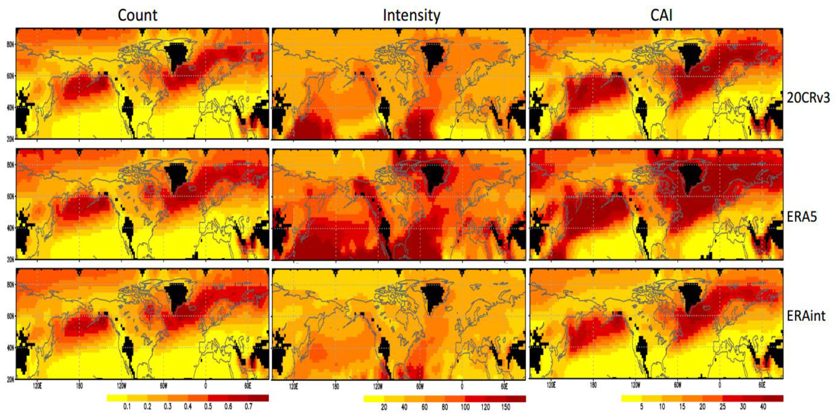
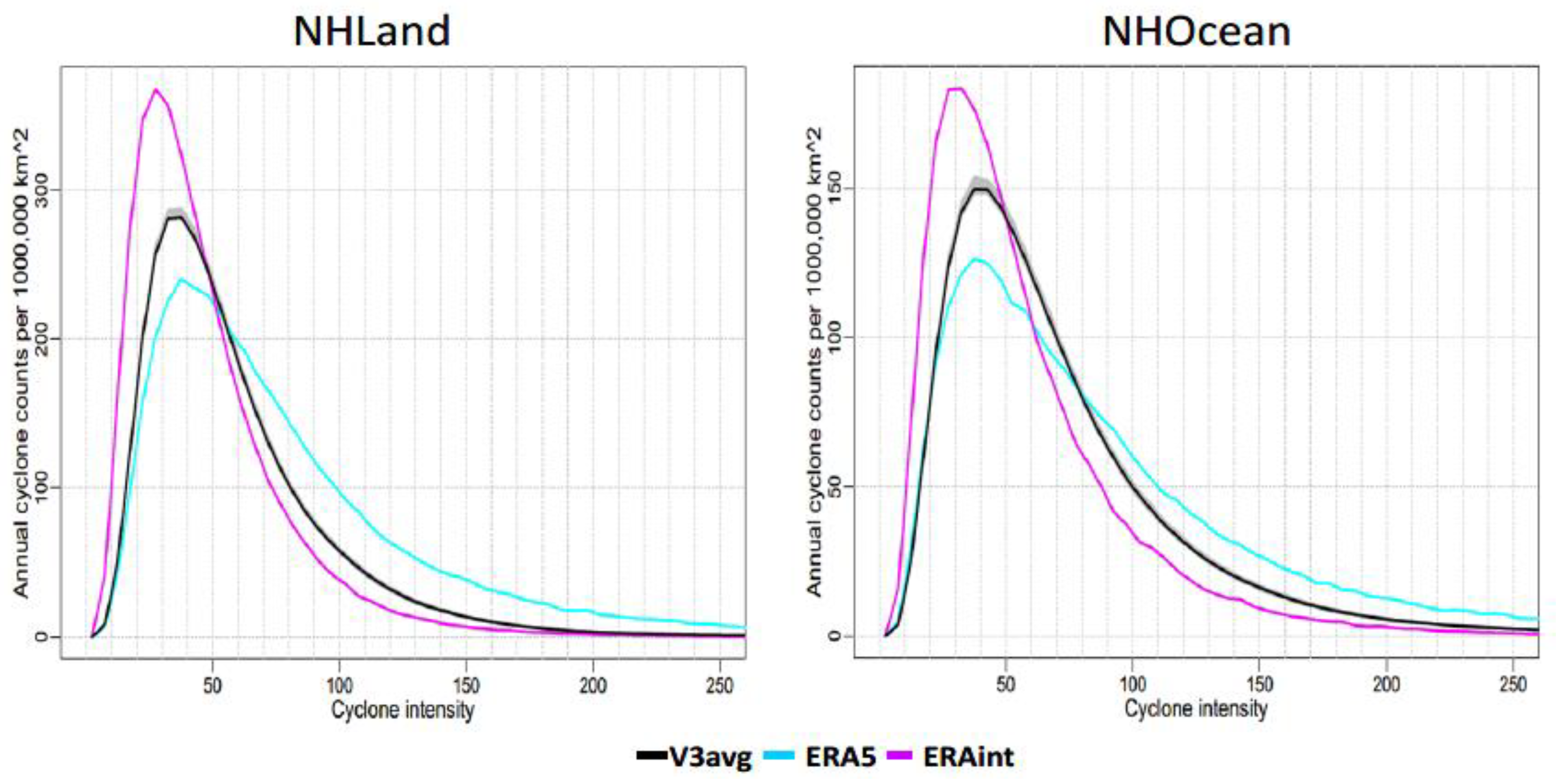
3.1. Climatology of Cyclone Activity

Figure 1 show the annual climatologies of the cyclone count, intensity, and CAI over the period 1981–2010 for 20CRv3, ERA5, and ERAint. In general, the climatological cyclone count displays two dominant regions of high cyclonic activities over the North Pacific and North Atlantic, with secondary centers over the Arabian Sea and Arctic (Figure 1, left panels). The dominant cyclone activity centers are consistent with those obtained using various tracking methods (e.g., [1,2,3]) and collocate with activity centers of the northern storm track regions (e.g., [18,49,50]). In contrast, the cyclone intensity reveals high values mainly in the subtropical coastal regions, especially the subtropical western and eastern Pacific and the Gulf of Mexico, with secondary centers along the western coast of Canada and around Iceland (Figure 1, middle panels). The subtropical cyclone intensity centers also collocate with active hurricanes and typhoons [51,52]. The climatological CAI resembles the cyclone count pattern (Figure 1, cf. right panels with left panels), with dominant action centers over the North Pacific and North Atlantic, as well as the subtropical western Pacific and the Arabian Sea. This indicates that CAI tends to be dominated by the cyclone count distribution.
Similar patterns of cyclonic activity can be seen in 20CRv3, ERA5, and ERAint products, especially for the cyclone count and CAI (Figure 1). The area weighted pattern correlations of the cyclone count within the northern extratropics (20–90° N) are close to 1.0 between 20CRv3 and either ERA5 or ERAint. The spatial correlation of CAI between 20CRv3 and ERA5 (ERAint) is 0.95 (0.93). The correlation is slightly higher between 20CRv3 and the mean of ERA5 and ERAint at 0.96. By contrast, the pattern correlations of the cyclone intensity are 0.74, 0.66 and 0.77, respectively, between 20CRv3 and ERA5, 20CRv3 and ERAint, and 20CRv3 and the average of ERA5 and ERAint.
Across the different reanalyses, the indices mainly differ in magnitude. For the cyclone count, values in 20CRv3 are slightly lower around Iceland and slightly higher over the Arabian Sea than those in the two ERA reanalyses. For the cyclone intensity, values in 20CRv3 are much lower than those in ERA5 over the subtropical region (20–30° N) and around Iceland, while values in 20CRv3 are much higher than those in ERAint over the subtropical western and eastern Pacific and the Gulf of Mexico. In addition, the cyclone intensity in 20CRv3 tends to be close to the average intensity of the two ERA products, with differences mainly in the subtropical region that are much smaller than those between 20CRv3 and either ERA5 or ERAint. For the CAI, values in 20CRv3 are lower than those in ERA5, mainly around Iceland, while values in 20CRv3 are higher than those in ERAint over the subtropical western Pacific and the Arabian Sea.
Figure 2 compare histograms of annual cyclone counts as a function of cyclone intensity over the northern extratropical land (within 20–90° N) and ocean (over 20–70° N) in the three datasets over the common period 1979–2015. In general, similar cyclone distributions can be seen over the extratropical land and ocean, with high counts for moderate-intensity cyclones. However, differences are also apparent in the three datasets. Cyclone counts in 20CRv3 are generally between those in ERA5 and ERAint for almost all intensity cyclones, especially over the northern extratropical land. Specifically, over the northern land (Figure 2, left), 20CRv3 has more cyclones than ERA5 and fewer than ERAint for low and moderate intensity cyclones (lower than 60 ∗ 10−5 hPa km−2), while it has more strong cyclones than ERAint and fewer than ERA5 for high-intensity cyclones (higher than 60 × 10−5 hPa km−2). Over the northern ocean (Figure 2, right), 20CRv3 has fewer low and moderate intensity cyclones (lower than 60 × 10−5 hPa km−2) and more strong cyclones than ERAint, while it has similar weak cyclones (lower than 20 × 10−5 hPa km−2), more moderate intensity cyclones (20–80 × 10−5 hPa km−2), and fewer strong cyclones (higher than 80 × 10−5 hPa km−2) than ERA5. In addition, the ensemble spread of the 80 members in 20CRv3 is low, indicating the robustness of the results.
Overall, there is a general agreement of the cyclone climatologies in the three datasets, especially for the spatial distribution. Differences in the cyclone activity strength among the datasets may be partially attributed to the influence of various spatial resolutions in the reanalysis data, which in turn affects cyclone identification and tracking methods [1,26]. In addition, 20CRv3 assimilates the IBTrACS (International Best Track Archive for Climate Stewardship) central pressure data that provides global tropical cyclone best track data [53], while the ERA reanalyses do not. Other factors, such as the dynamics, parameterizations, and assimilation schemes implemented in various reanalysis models, would also result in differences in cyclone activity [1,31,33]. 20CRv3 and ERA reanalyses are generated by substantially different models as described above in Sect. 2. Hence, it is not a surprise that differences exist even between 20CRv3 and ERAint, despite their having similar horizontal resolutions in the assimilating model.

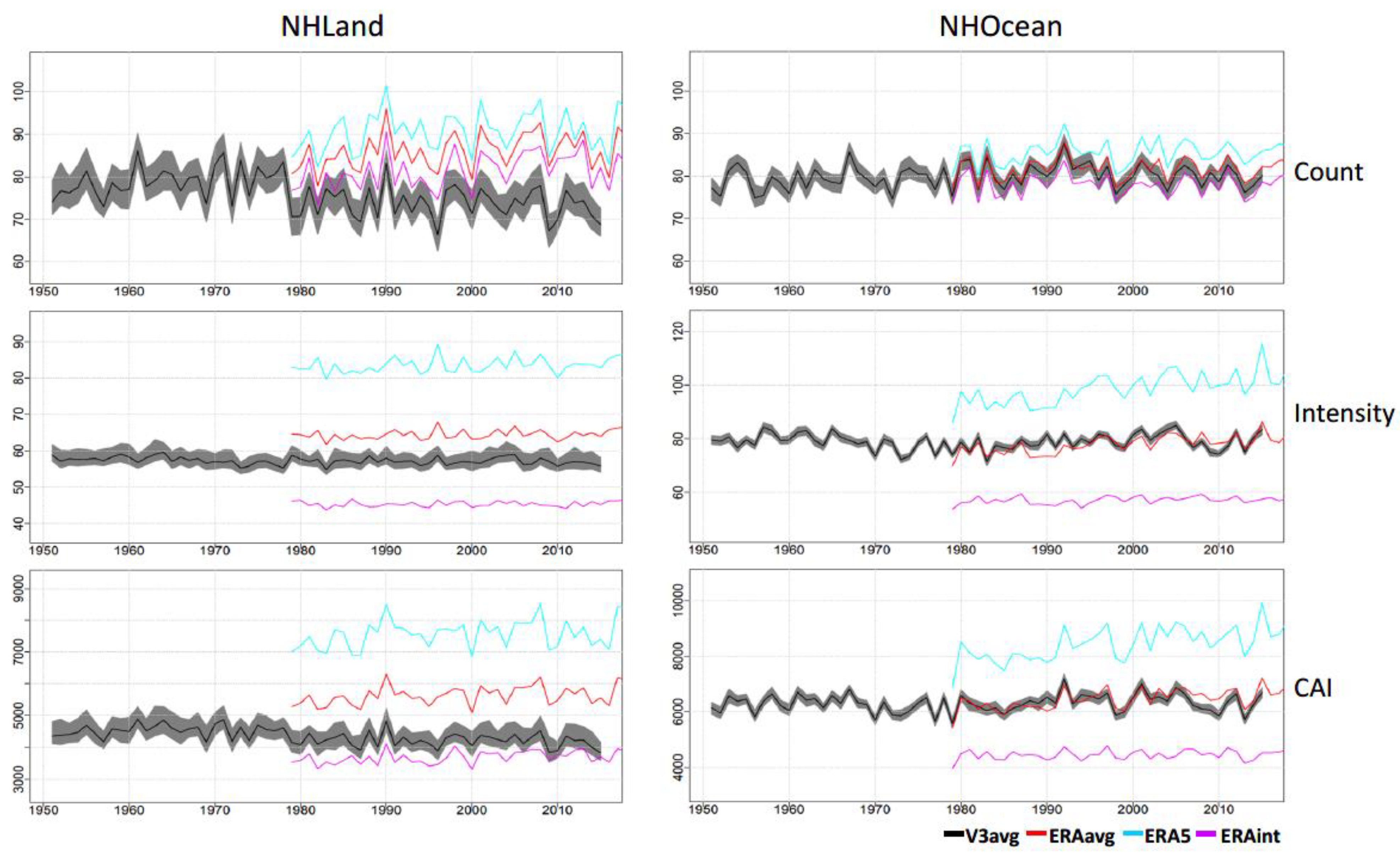
3.2. Variation of Cyclone Activity

Figure 3 present variations of the annual mean cyclone count, intensity, and CAI averaged over the northern extratropical land (left panels) and ocean (right panels). The ensemble average and spread of the cyclone indices are shown for 20CRv3 over the period 1951–2015. Here, the ensemble spread is quantified by the ensemble standard deviation among the 80 ensemble members. Results from ERAint and ERA5, one integration each, as well as their average (ERAavg) over the period 1979–2018, are also shown. Variations of the ensemble averages of the three indices reveal long-term trends as well as interannual–interdecadal variability (Figure 3). Over the overlapping period 1979–2015, the interannual variability of the 20CRv3 indices averaged over the northern land and ocean resembles the ERA results, which are qualitatively consistent in ERAint and ERA5. The temporal correlations of the regional mean indices between the 20CRv3 ensemble average and either ERAint or ERA5 are above 0.65, except for relatively lower correlations of the regional mean cyclone intensity (about 0.45) between 20CRv3 and ERAint, over the northern land and ocean. All these correlations are statistically significant at the 5% level over the 37-year period. The correlations between 20CRv3 and ERAavg are higher than those between 20CRv3 and individual ERA series. Differences in the cyclonic activity indices between 20CRv3 and either ERA5 or ERAint are mainly seen in the cyclone index magnitudes, especially for the cyclone intensity index. The index magnitudes in recent decades in 20CRv3 are comparable to that from ERAint for the cyclone count and CAI over the northern land and to ERAavg for the cyclone intensity over the northern land and for all indices considered over the northern ocean (Figure 3).
For the northern extratropical land mean, the ratio of ensemble spread to ensemble average in 20CRv3 ranges from 2.1% to 3.4%, with an average of 2.8%, for the cyclone count over the period 1951–2015. The ratio is even lower for the cyclone intensity than the cyclone count, ranging from 1.4% to 3.0%, with an average of 2.1%. Hence, the ratio for CAI is also low, with an average of 4.2% over 65 years (Figure 3, left panels and Table 1). Similarly, the ratios are low for the northern extratropical ocean, with averages of 1.4%, 1.0%, and 1.6% for the cyclone count, intensity, and CAI, respectively (Figure 3, right panels and Table 1). The high agreement among ensemble members indicates the low uncertainty of the northern cyclone activity indices due to internal climate variability. The low ratio in the cyclone variation also implies a high signal-to-noise ratio, which is defined as the ratio of the ensemble average to ensemble standard deviation and measures the level of the desired signal to the level of background noise.
Seasonal changes in cyclone activity are further quantified by analyzing variations of the indices in four seasons. For the northern extratropical land (Figure 4), magnitudes of the cyclone count and CAI are stronger in warm seasons (AMJ and JAS) than in cold seasons (JFM and OND). This is consistent with previous studies [2], which show an increasing number of cyclones over the continental storm track region in summer. However, magnitudes of cyclone intensity tend to be stronger in cold seasons than in warm seasons (Figure 4, middle panels). The spread in the seasonal indices, including the three cyclone indices, reveals higher values in warm seasons than in cold seasons (Figure 4). In addition, similar to the annual mean result, the ratios of ensemble spread to ensemble average are higher in the cyclone count and CAI than the cyclone intensity (Table 1). By contrast, for the northern extratropical ocean (Figure 5), the magnitudes of the cyclone count are generally stronger in cold seasons than in warm seasons. This is also in agreement with previous findings that there is an enhancement of the oceanic storm track in winter [2]. The ratios of ensemble spread to ensemble average of the seasonal cyclone indices are also higher in warm seasons than cold seasons and higher in the cyclone count and CAI than the cyclone intensity (Table 1 and Figure 5). In addition, the seasonal variations of the 20CRv3 cyclone indices over the northern land and ocean are also comparable to those in the ERA reanalyses over the period 1979–2015, in terms of the interannual variability, with differences mainly seen in the cyclone index magnitude. These are similar to those seen above in the annual mean result (cf., Figure 4 and Figure 5 with Figure 3).
The annual and seasonal variations of the cyclone activity indices averaged over the northern extratropical land and ocean are examined above. The general features obtained over the northern land can be seen in both Eurasian and North American continents (not shown), including stronger magnitudes of the cyclone count in warm seasons than in cold seasons, lower ratios of ensemble spread to ensemble average in the cyclone intensity than in the cyclone count, higher spreads in warm seasons than in cold seasons, and comparable annual and seasonal cyclone activities in 20CRv3 and the ERA products over the period 1979–2015. Likewise, the features obtained over the northern ocean are seen over both the North Pacific and North Atlantic oceans (not shown).

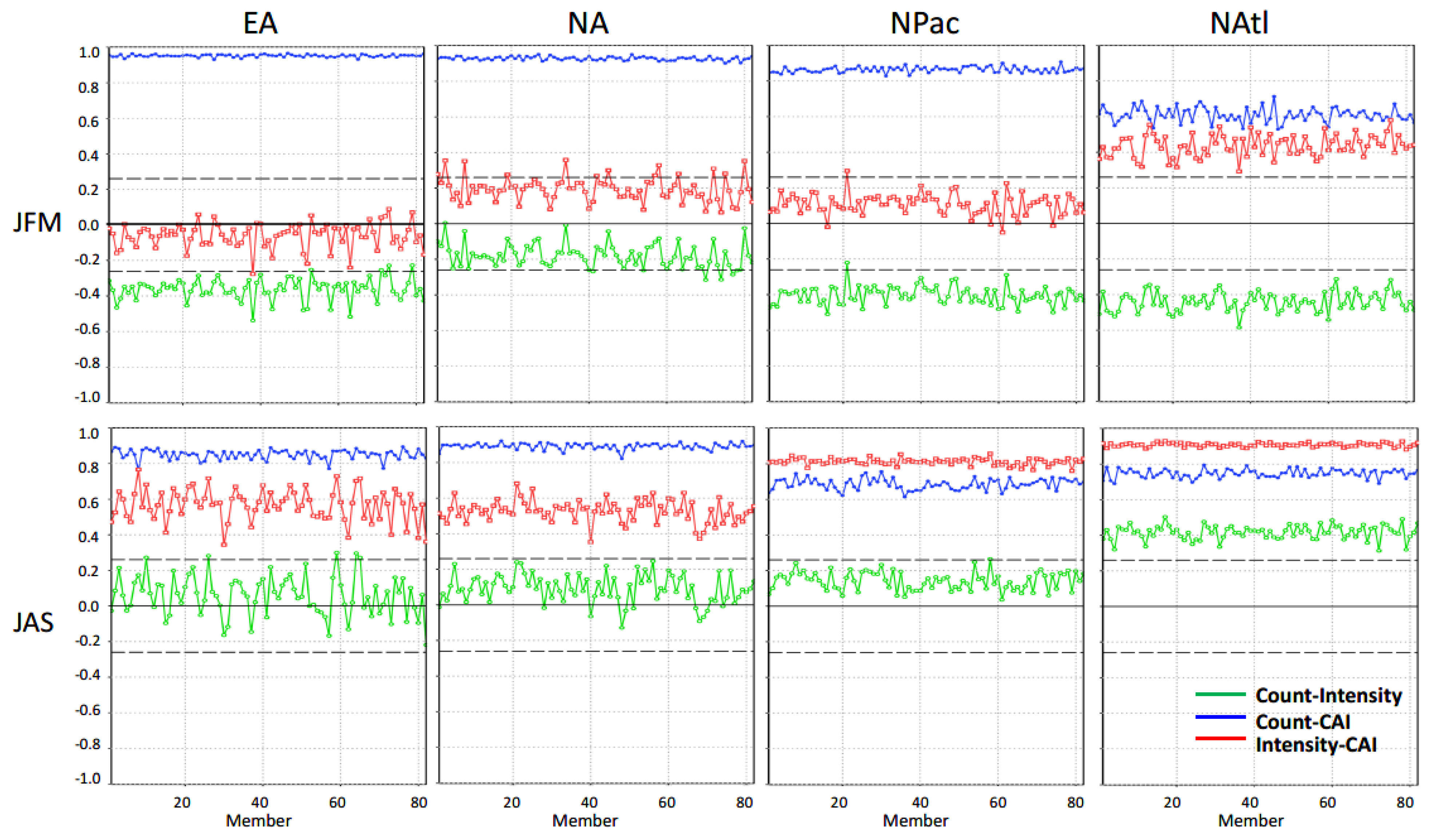
3.3. Relationship between Regional Mean Cyclone Indices

To explore the relationship between the cyclone activity indices, we analyze temporal correlations among the three indices in 20CRv3, using data over the period 1951–2010. We focus on the correlations calculated using the cyclone indices averaged over the northern continents of Eurasia (EA) within (20°–90° N, 20° W–170° W) and North America (NA) within (20°–90° N, 170°–50° W), and over the extratropical oceans within 20–70° N of the North Pacific (NPac) and North Atlantic (NAtl).
Figure 6 display the correlations among the seasonal cyclone indices in JFM and JAS calculated from the 80 ensemble members, the average of the 80 correlations, and the correlation calculated from the ensemble average indices. The highest and statistically significant correlation is positive and seen between the cyclone count and CAI over all four regions in JFM (with values above 0.80 in EA, NA, and NPac and above 0.50 in NAtl) and over the two continents in JAS (with values above 0.80). The correlation between the cyclone count and CAI over the two ocean regions is also above 0.60 and statistically significant, although slightly higher correlations are apparent there between the cyclone intensity and CAI. The correlation between the cyclone intensity and CAI is positive and statistically significant over all four regions in JAS and over the NAtl in JFM. However, the JFM correlation between the cyclone intensity and CAI is generally weak and mainly positive in the NA and NPac and negative in EA. The temporal relationships further indicate that the combined index CAI tends to be dominated by the cyclone count.
The cyclone count is negatively correlated with the cyclone intensity in JFM (Figure 6), with significant correlations (around −0.4) in EA, the NPac, and NAtl. By contrast, the correlations between the cyclone count and intensity in JAS tend to be positive but statistically insignificant, except in the NAtl (around 0.4).
Table 2 further list the average and standard deviation of the 80 correlations calculated from the ensemble members and the correlation calculated from ensemble average indices over the four regions. It is interesting to see from Table 2 that the average of the 80 correlations is much higher than its standard deviation, especially for statistically significant correlation coefficients, indicating high signal-to-noise ratios of the results. In addition, the average of the 80 correlations is close to the correlation calculated using the ensemble average indices, especially for the statistically significant correlations. This indicates the robustness of the relationships and implies the ensemble average index can be used to characterize the regional mean cyclone activity.

4. Relationship of Extreme Temperatures to Regional Mean Cyclone Activity

To explore the linkage of cyclone activity and extreme temperatures, we analyze the relationships between the indices of regional mean cyclone activity and the principal modes of cold and warm extreme temperatures over Eurasia and North America in JFM and JAS. We also calculate extreme temperature anomalies explained by cyclone activity over the two continents. In addition, we examine the anomalies of large-scale atmospheric circulation and the induced temperature advection associated with cyclone activity to aid in understanding the physical mechanism linking cyclone activity and extreme temperature anomalies.

4.1. Relations between Cyclone Activity and Continental Extreme Temperatures

The principal mode of the extreme temperature variability is identified by EOF analyses of area-weighted extreme temperature index anomalies over the land grids in Eurasia within (20°–80° N, 20° W–180° E) and North America within (20°–80° N, 170°–50° W), separately, in JFM and JAS.
In JFM, the principal modes (EOF1s) account for about 32–36% of the total interannual cold and warm extreme variances over Eurasia (Figure 7, left panels) and are well separated from their subsequent EOFs as per the criterion of North et al. [54]. EOF1 of the cold extreme (TN10 and TX10) anomalies tends to be dominated by a large anomaly over the domain of interest, with the center of action located over Kazakhstan and south Russia and accompanied by a weak anomaly of the opposite sign over south Asia. EOF1 of the warm extreme (TN90 and TX90) anomalies also reveals a large anomaly over northern parts of the continent, with the action center over Kazakhstan and extending to south Europe and south Russia, together with a relatively weak anomaly of the opposite sign over south Asia. The corresponding principal components (PC1s) are then used to characterize the leading cold and warm extreme variability. The correlations between the PC1s and the three cyclone indices averaged over Eurasia in the 80 ensemble members in 20CRv3 are calculated and shown in Figure 8. In general, positive (negative) correlations are seen between the cyclone count and PC1s of warm (cold) extreme anomalies (Figure 8, top-left panels). Similarly, positive (negative) correlations are found between the CAI and PC1s of warm (cold) extreme anomalies (Figure 8, top-right panels). In contrast, cyclone intensity and PC1s of warm (cold) extreme anomalies correlate negatively (positively) (Figure 8, top-middle panels). The average of the 80 correlations is much higher than its standard deviation, indicating the robustness of the relationships. Additionally, the average of the 80 correlations is close to the correlation calculated using the ensemble average cyclone index and the PC1 of extreme temperature anomalies (Table 3). The highest correlation is found between the cyclone count and the leading extreme temperature variability, with significant correlations of about 0.60 (−0.40) between the cyclone count and PC1s of warm (cold) extreme anomalies. The relations are also clearly evident in the JFM extreme temperature anomalies regressed upon the regional mean cyclone count index, which reveal prominent anomalies collocating with the action centers in the corresponding EOF1 patterns (cf. Figure 7 right panels with left panels).
Over North America, EOF1s account for about 29–37% of the total interannual extreme temperature variances in JFM (Figure 9, left panels) and are also separated from the subsequent EOFs according to the criterion [54]. The two EOF1 patterns for cold extreme (TN10, TX10) anomalies are each dominated by a large anomaly over western–central Canada and the northwestern US. EOF1 of the warm night extreme (TN90) anomalies show a large anomaly over central Canada, while EOF1 of the warm day extreme (TX90) anomalies in JFM reveal a large anomaly over western–central Canada and the northwestern US. EOF1s of both TN90 and TX90 anomalies are also accompanied by a relatively weak anomaly of the opposite sign over Mexico and the southeastern US. The leading patterns of extreme temperature variability are consistent with [55], based on combined EOF analyses of December–January–February (DJF) mean extreme cold and warm anomalies, indicating the robustness of the dominant, extreme temperature variability in winter.
We then calculate the correlations between the corresponding PC1s and the three cyclone indices averaged over North America in the 80 ensemble members (Figure 8, lower panels). Surprisingly different from the results over Eurasia, significant correlations are mainly seen between the cyclone intensity and PC1s of extreme temperature anomalies, with positive correlations (about 0.40) between the cyclone intensity and PC1s of cold extreme anomalies and negative correlations (about −0.35 to −0.55) between the cyclone intensity and PC1s of warm extreme anomalies. The average of the 80 correlations is again much higher than its standard deviation and is close to the correlation calculated using the ensemble average cyclone index and the PC1 of extreme temperature anomalies (Table 3). The relations between the cyclone intensity and PC1s of extreme temperature anomalies are also clear in the JFM extreme temperature anomalies regressed upon the regional mean cyclone intensity index (Figure 9, right panels), which show prominent anomalies generally collocating with the action centers in the corresponding EOF1 patterns (cf. right panels with left panels in Figure 9). By contrast, correlations between the PC1s of extreme temperature anomalies and either the cyclone count or CAI are low and not significant in JFM, except the relationship between the cyclone count and PC1 of TX10 anomalies that is marginally significant at the 5% level (Figure 8). It remains to be explored why correlations between the cyclone count index and the principal component of JFM extreme temperature anomalies are significant over Eurasia and insignificant over North America.
The relationship between the regional mean cyclone activity and continental extreme temperature variability in JFM can be further quantified by calculating the percentage of local temperature variance explained by a cyclone index, following Equations (1) and (2). Here, we use the regionally averaged ensemble mean cyclone count as the index over Eurasia and the regionally averaged ensemble mean cyclone intensity index over North America. Respectively, these have the strongest correlation between cyclone activity and leading modes of extreme temperature anomalies, as discussed above.
Over Eurasia, cyclone count explains about 5–20% of the interannual cold extreme variance and about 10–45% of warm extreme variance over half of the continent (Figure 10, left panels), with high percentage centers generally following the action centers apparent in the corresponding regression anomalies (Figure 7, right panels). Averaging over continental Eurasia (following Equation (2)), cyclone activity explains 8.2%, 8.4%, 17.2%, and 21.2% of TN10, TX10, TN90, and TX90 variance, respectively, in JFM. Similarly, over North America, the cyclone intensity explains about 10–20% of interannual cold, extreme variances and about 5–40% of warm extreme variances in JFM over half of the continent (Figure 10, right panels), with high percentages also following the action centers of the corresponding regressions (Figure 9, right panels). Averaging over the continent, cyclone activity explains 9.3%, 9.8%, 12.6%, and 8.5% of TN10, TX10, TN90, and TX90 variance, respectively.
In JAS, the four EOF1s account for 18–26% of the total interannual extreme temperature variances over Eurasia and 26–29% over North America (not shown), slightly lower than the corresponding percentages explained in JFM. These principal modes are also separated from their subsequent EOFs. However, the correlations between the leading cold and warm extreme variability and the three cyclone indices are low in JAS, with magnitudes lower than 0.20 for all correlations over Eurasia and North America. These are not statistically significant at the 5% level. The consistently low correlations obtained using the cyclone indices of each of the 80 members and the ensemble average indicate the robustness of the poor relationship in summer between cyclone activity and leading modes of temperature extremes over Eurasia and North America.

4.2. The Cyclone Activity Associated Large-Scale Circulation and Temperature Advection Anomalies

Figure 11 display the anomalies of MSLP (top panels) and horizontal winds and temperature advection (Fadv, following Equation (3)) at 850-hPa (bottom panels) in JFM regressed upon the regionally averaged ensemble mean cyclone count index over Eurasia and cyclone intensity index over North America. Over Eurasia, in association with a positive anomaly of the cyclone count index, there is a pronounced negative MSLP anomaly apparent over most of Eurasia, with the center of action over the Northern European Plain, together with a relatively weak positive MSLP anomaly over Southern Europe (Figure 11, top-left). The anomalous large-scale circulation induces the exchange of mid–high latitude air over Eurasia, which implies temperature advection anomalies contributing to temperature anomalies. Specifically, accompanying the MSLP anomalies, there are anomalous western–northwestern winds over Europe, southwestern wind anomalies over the West Siberian Plain, and westerly wind anomalies over south Russia. The anomalous winds induce warm advection over most of Eurasia, in particular Kazakhstan and south Russia (Figure 11, bottom-left). In addition, the anomalous Fadv has comparable contributions from both the anomalous zonal and meridional wind-related advection components over the West Siberian Plain and is dominated by its zonal wind-related component over Europe and south Russia (not shown). This indicates the crucial role of winds in the anomalous thermal advection. The temperature advection anomalies collocate with the action centers of warm extreme increase and cold extreme decrease over Eurasia (Figure 7), suggesting that the thermal advection drives the temperature anomalies.
On the other hand, in association with a positive anomaly of the cyclone intensity index over North America, MSLP is dominated by a pronounced positive anomaly over northwestern parts of North America, with the action center over the northeastern Pacific, together with a slight MSLP decrease over northeastern Canada and increase over the southeastern US (Figure 11, top-right). Accompanying these circulation anomalies, there are anomalous northerly winds over western–central Canada, the northwestern US, and eastern Canada, along with southwestern wind anomalies over the southeastern US. The anomalous winds induce cold advection over most of Canada and the northwestern US, as well as warm advection over the southeastern US (Figure 11, bottom-right). The anomalous Fadv is dominated by its meridional wind-related component over North America (not shown). The temperature advection anomalies collocate with the warm extreme decrease and cold extreme increase over northern parts of North America, as well as the warm extreme increase and cold extreme decrease over Mexico and the southeastern US (Figure 9).
Overall, the collocation between the thermal advection and prominent extreme temperature anomalies in JFM suggests that the circulation anomalies associated with cyclone activity and the induced temperature advection in the lower troposphere contribute to the variability of temperature extremes over Eurasia and North America.
The large-scale circulation and thermal advection anomalies associated with cyclone activity in JAS are weak and statistically insignificant over the two study regions (not shown). This suggests that the summertime temperature anomalies are associated with local thermodynamic processes, via surface radiative and turbulent heat flux anomalies [7,8,56], or with other aspects of the circulation (such as blocking). Hence, the relationship between cyclone activity and extreme temperature variability is weak in JAS over the two continents, as discussed above in Section 4.1.

5. Summary

In this study, we detected and tracked extratropical cyclones by focusing on large-scale features of cyclone activity and applying a modified version of the objective cyclone tracking algorithm on 6-hourly MSLP data extracted from three reanalysis datasets, 20CRv3 over the period 1951–2015 and ERAint and ERA5 over the period 1979–2018. Three indices are considered to characterize cyclone activity: cyclone count, cyclone intensity, and a combined index CAI. We analyzed the northern extratropical cyclone activity in 20CRv3 by examining the annual climatology and seasonal variations of the three cyclone indices and compared them with those in the ERA datasets for the common period 1979–2015. We examined the temporal relationship between the cyclone indices over continental Eurasia and North America and the extratropical North Pacific and North Atlantic oceans. The robustness of these relationships was assessed by analyzing all 80 ensemble members in 20CRv3. We then explored the linkage of cyclone activity in 20CRv3 and observed cold and warm extremes over Eurasia and North America, based on the overlapping period 1951–2010. In addition, we examined the dynamics linking cyclone activity and continental extreme temperature anomalies.
There was a general agreement between the cyclone index climatologies in 20CRv3 and ERA reanalysis datasets, especially for the spatial pattern of the cyclone indices over the northern extratropics. The climatological annual cyclone count revealed two dominant regions of high cyclonic activities over the North Pacific and North Atlantic, collocating with activity centers of the northern storm track. The cyclone intensity showed high values mainly in the subtropical coastal regions, especially the subtropical western and eastern Pacific and the Gulf of Mexico, collocating with active hurricanes and typhoons. The climatological CAI tended to be dominated by the cyclone count distribution. Differences among these reanalysis products mainly appeared in the cyclone index magnitude and were attributed to the influence of various spatial resolutions in the reanalysis data as well as differences in model structure, assimilation algorithms, and assimilated observations. In addition, the interannual variability of regional mean annual and seasonal cyclone indices over the northern extratropical land and ocean was comparable between 20CRv3 and the ERA reanalyses in recent decades. Over Eurasia and North America, the cyclone count and CAI were stronger in warm seasons than in cold seasons, while the cyclone intensity tended to be stronger in cold seasons than in warm seasons. Over the North Pacific and North Atlantic, the cyclone count was generally stronger in cold seasons than in warm seasons. High agreement of the cyclone activity variation was seen in the 80 ensemble members in 20CRv3. Nevertheless, higher ensemble spreads of the cyclone indices appeared in warm seasons than in cold seasons over the northern extratropical land and ocean.
Cyclones are complex phenomena that vary in intensity, duration, location, frequency, and vertical structure. Temporal correlations between regional mean cyclone indices indicate that cyclone count and intensity are negatively correlated in JFM, with correlations significant at the 5% level over Eurasia and the North Pacific and North Atlantic. By contrast, cyclone count and intensity tend to be positively correlated in JAS. However, these positive correlations are weak and statistically insignificant, except for those over the North Atlantic. The interannual CAI variability is dominated by the cyclone count variability. The relationships are robust, as seen from the 80 ensemble members. In addition, the ensemble average cyclone index can be used to characterize regional mean cyclone activity.
Observed cold and warm extreme anomalies over the northern continents were found to be closely associated with cyclone activity. Over Eurasia and North America, the principal component corresponding to the leading mode of warm (cold) extreme anomalies in JFM was positively (negatively) correlated with the cyclone count and negatively (positively) correlated with the cyclone intensity. The principal component had the strongest correlation with the cyclone count index over Eurasia and the cyclone intensity index over North America. The relationships are robust, as seen by all ensemble members. In general, temperature anomalies associated with cyclone count explain about 10% of interannual cold, extreme variances and about 20% of warm extreme variances in JFM on the continental average over Eurasia. Similarly, temperature anomalies associated with cyclone intensity explain about 10% of interannual cold and warm extreme variances on average over North America. In winter, the cyclone activity associated with large-scale atmospheric circulation anomaly and its induced temperature advection in the lower troposphere drive temperature anomalies over Eurasia and North America. In summer, by contrast, the circulation and thermal advection anomalies associated with cyclone activity are weak over the two continents. The temperature anomalies there tend to be supported by local thermodynamic processes. Hence, the relationship between cyclone activity and extreme temperature variability is weak over Eurasia and North America in summer.

Author Contributions

B.Y. and X.L.W. designed and carried out the analysis. Y.F. and R.C. created cyclone data and helped with the analysis. B.Y. wrote the manuscript. methodology, G.P.C. and L.C.S.; review and editing paper, G.P.C., L.C.S., P.D.S., M.W. and X.-Y.Y.; validation, G.P.C. All authors have read and agreed to the published version of the manuscript.

Funding

GPC: LCS and PDS were supported in part by the NOAA Cooperative Agreement with CIRES, NA17OAR4320101 and by the NOAA Physical Sciences Laboratory. Support for the Twentieth Century Reanalysis Project version 3 dataset was provided by the U.S. Department of Energy, Office of Science Biological and Environmental Research (BER), the National Oceanic and Atmospheric Administration Climate Program Office, and the NOAA Physical Sciences Laboratory. The NOAA-CIRES-DOE Twentieth Century Reanalysis Project version 3 used resources of the National Energy Research Scientific Computing Center (NERSC) managed by Lawrence Berkeley National Laboratory, which is supported by the Office of Science of the U.S. Department of Energy under Contract No. DE-AC02-05CH11231 and used resources of NOAA’s Remotely Deployed High-Performance Computing Systems.

Data Availability Statement

Data used in this study are described in Section 2.

Acknowledgments

We thank Jeffrey S. Whitaker and three anonymous reviewers for their constructive suggestions and comments, which helped to improve the study. The 20CRv3 ensemble member fields were provided by the NERSC Science Gateway.

Conflicts of Interest

The authors declare no conflict of interest.

References

  1. Ulbrich, U.; Leckebusch, G.C.; Pinto, J.G. Extra-tropical cyclones in the present and future climate: A review. Theor. Appl. Climatol. 2009, 96, 117–131. [Google Scholar] [CrossRef] [Green Version]
  2. Tilinina, N.; Gulev, S.K.; Rudeva, I.; Koltermann, P. Comparing cyclone life cycle characteristics and their interannual variability in different reanalyses. J. Clim. 2013, 26, 6419–6438. [Google Scholar] [CrossRef] [Green Version]
  3. Varino, F.; Arbogast, P.; Joly, B.; Riviere, J.; Fandeur, M.-L.; Bovy, H.; Granier, J.-B. Northern Hemisphere extratropical winter cyclones variability over the 20th century derived from ERA-20C reanalysis. Clim. Dyn. 2019, 52, 1027–1048. [Google Scholar] [CrossRef]
  4. Favre, A.; Gershunov, A. Extra-tropical cyclonic/anticyclonic activity in North Eastern Pacific and air temperature extremes in Western North America. Clim. Dyn. 2006, 26, 617–629. [Google Scholar] [CrossRef]
  5. Wang, X.L.; Swail, V.R.; Zwiers, F.W. Climatology and changes of extratropical cyclone activity: Comparison of ERA-40 with NCEP-NCAR reanalysis for 1958–2001. J. Clim. 2006, 19, 3145–3166. [Google Scholar] [CrossRef]
  6. Wang, X.L.; Feng, Y.; Compo, G.P.; Swail, V.R.; Zwiers, F.W.; Allan, R.J.; Sardeshmukh, P.D. Trends and low frequency variability of extra-tropical cyclone activity in the ensemble of twentieth century reanalysis. Clim. Dyn. 2013, 40, 2775–2800. [Google Scholar] [CrossRef]
  7. Chang, E.K.M.; Ma, C.G.; Zheng, C.; Yau, A.M.W. Observed and projected decrease in Northern Hemisphere extratropical cyclone activity in summer and its impacts on maximum temperature. Geophys. Res. Lett. 2016, 43, 2200–2208. [Google Scholar] [CrossRef] [Green Version]
  8. Sillmann, J.; Thorarinsdottir, T.; Keenlyside, N.; Schaller, N.; Alexander, L.V.; Hegerl, G.; Seneviratne, S.I.; Vautard, R.; Zhang, X.; Zwiers, F.W. Understanding, modeling and predicting weather and climate extremes: Challenges and opportunities. Wea. Clim. Ext. 2017, 18, 65–74. [Google Scholar] [CrossRef]
  9. Ulbrich, U.; Brücher, T.; Fink, A.H.; Leckebusch, G.C.; Krüger, A.; Pinto, J.G. The central European floods in August 2002: Part I—Rainfall periods and flood development. Weather 2003, 58, 371–376. [Google Scholar] [CrossRef] [Green Version]
  10. Ashley, W.S.; Black, A.W. Fatalities associated with nonconvective high wind events in the United States. J. Appl. Meteorol. Climatol. 2008, 47, 717–725. [Google Scholar] [CrossRef]
  11. Colle, B.A.; Buonaiuto, F.; Bowman, M.J.; Wilson, R.E.; Flood, R.; Hunter, R.; Mintz, A.; Hill, D. New York city’s vulnerability to coastal flooding. Bull. Am. Meteorol. Soc. 2008, 89, 829–841. [Google Scholar] [CrossRef] [Green Version]
  12. Fink, A.H.; Brücher, T.; Ermert, V.; Krüger, A.; Pinto, J.G. The European storm Kyrill in January 2007: Synoptic evolution, meteorological impacts and some considerations with respect to climate change. Nat. Hazards Earth Syst. Sci. 2009, 9, 405–423. [Google Scholar] [CrossRef] [Green Version]
  13. Pinto, J.G.; Zacharias, S.; Fink, H.; Leckebusch, G.C.; Ulbrich, U. Factors contributing to the development of extreme North Atlantic cyclones and their relationship with the NAO. Clim. Dyn. 2009, 32, 711–737. [Google Scholar] [CrossRef] [Green Version]
  14. Kunkel, K.E.; Easterling, D.R.; Kristovich, D.A.R.; Gleason, B.; Stoecker, L.; Smith, R. Meteorological causes of the secular variations in observed extreme precipitation events for the conterminous United States. J. Hydrometeorol. 2012, 13, 1131–1141. [Google Scholar] [CrossRef]
  15. Hawcroft, M.K.; Shaffrey, L.C.; Hodges, K.I.; Dacre, H.F. How much Northern Hemisphere precipitation is associated with extratropical cyclones? Geophys. Res. Lett. 2012, 39, L24809. [Google Scholar] [CrossRef] [Green Version]
  16. Pfahl, S.; Wernli, H. Quantifying the relevance of cyclones for precipitation extremes. J. Clim. 2012, 25, 6770–6780. [Google Scholar] [CrossRef]
  17. Serreze, M.C.; Carse, F.; Barry, R.G.; Rogers, J.C. Icelandic Low cyclone activity: Climatological features, linkages with the NAO and relationships with recent changes elsewhere in the Northern Hemisphere circulation. J. Clim. 1997, 10, 453–464. [Google Scholar] [CrossRef]
  18. Hoskins, B.J.; Hodges, K.I. New perspectives on the northernhemisphere winter storm tracks. J. Atmos. Sci. 2002, 59, 1041–1061. [Google Scholar] [CrossRef]
  19. König, W.; Sausen, R.; Sielmann, F. Objective identification of cyclones in GCM simulations. J. Clim. 1993, 6, 2217–2231. [Google Scholar] [CrossRef] [Green Version]
  20. Zhang, X.D.; Walsh, J.E.; Zhang, J.; Bhatt, U.S.; Ikeda, M. Climatology and interannual variability of arctic cyclone activity 1948–2002. J. Clim. 2004, 17, 2300–2317. [Google Scholar] [CrossRef]
  21. Barnes, E.A.; Screen, J.A. The impact of Arctic warming on the midlatitude jet-stream: Can it? Has it? Will it? Wiley Interdiscip Rev. Clim. Change 2015, 6, 277–286. [Google Scholar] [CrossRef] [Green Version]
  22. Thompson, D.W.J.; Wallace, J.M. The Arctic Oscillation signature in the wintertime geopotential height and temperature fields. Geophys. Res. Lett. 1998, 25, 1297–1300. [Google Scholar] [CrossRef] [Green Version]
  23. Corti, S.; Molteni, F.; Palmer, T. Signature of recent climate change in frequencies of natural atmospheric circulation regimes. Nature 1999, 398, 799–802. [Google Scholar] [CrossRef]
  24. Raible, C.C.; Della-Marta, P.; Schwierz, C.; Wernli, H.; Blender, R. Northern hemisphere extratropical cyclones: A comparison of detection and tracking methods and different reanalyses. Mon. Wea. Rev. 2008, 136, 880–897. [Google Scholar] [CrossRef] [Green Version]
  25. Neu, U.; Akperov, M.G.; Bellenbaum, N.; Benestad, R.; Blender, R.; Caballero, R.; Cocozza, A.; Dacre, H.F.; Feng, Y.; Fraedrich, K.; et al. IMILAST—A community effort to intercompare extratropical cyclone detection and tracking algorithms. Bull. Amer. Meteor. Soc. 2013, 94, 529–547. [Google Scholar] [CrossRef]
  26. Wang, X.L.; Feng, Y.; Chan, R.; Isaac, V. Inter-comparison of extra-tropical cyclone activity in nine reanalysis datasets. Atmos. Res. 2016, 181, 133–153. [Google Scholar] [CrossRef] [Green Version]
  27. Chang, E.K.M.; Yau, A.M.W. Northern Hemisphere winter storm track trends since 1959 derived from multiple reanalysis datasets. Clim. Dyn. 2015, 47, 1435–1454. [Google Scholar] [CrossRef]
  28. Sinclair, M.R.; Watterson, I.G. Objective assessment of extra-tropical weather systems in simulated climates. J. Clim. 1999, 12, 3467–3485. [Google Scholar] [CrossRef] [Green Version]
  29. Simmonds, I.; Keay, K. Mean Southern Hemisphere extratropical cyclone behavior in the 40-year NCEP–NCAR reanalysis. J. Clim. 2000, 13, 873–885. [Google Scholar] [CrossRef]
  30. McCabe, G.J.; Clark, M.P.; Serreze, M.C. Trends in Northern Hemisphere surface cyclone frequency and intensity. J. Clim. 2001, 14, 2763–2768. [Google Scholar] [CrossRef]
  31. Hodges, K.I.; Hoskins, B.J.; Boyle, J.; Thorncroft, C. A comparison of recent reanalysis datasets using objective feature tracking: Storm tracks and tropical easterly waves. Mon. Wea. Rev. 2003, 131, 2012–2037. [Google Scholar] [CrossRef]
  32. Rudeva, I.; Gulev, S.K. Composite analysis of North Atlantic extra-tropical cyclones in NCEP–NCAR reanalysis data. Mon. Wea. Rev. 2011, 139, 1419–1446. [Google Scholar] [CrossRef] [Green Version]
  33. Trigo, I.F. Climatology and interannual variability of storm-tracks in the Euro-Atlantic sector: A comparison between ERA-40 and NCEP/NCAR reanalyses. Clim. Dyn. 2006, 26, 127–143. [Google Scholar] [CrossRef]
  34. Bromwich, D.H.; Fogt, R.L.; Hodges, K.I.; Walsh, J.E. A tropospheric assessment of the ERA-40, NCEP, and JRA-25 global reanalyses in the polar regions. J. Geophys. Res. 2007, 112, D10111. [Google Scholar] [CrossRef] [Green Version]
  35. Allen, J.T.; Pezza, A.B.; Black, M.T. Explosive cyclo-genesis: A global climatology comparing multiple reanalyses. J. Clim. 2010, 23, 6468–6484. [Google Scholar] [CrossRef]
  36. Hodges, K.I.; Lee, R.W.; Bengtsson, L. A comparison of extra-tropical cyclones in recent reanalyses ERA-Interim, NASA MERRA, NCEP CFSR, and JRA-25. J. Clim. 2011, 24, 4888–4906. [Google Scholar] [CrossRef]
  37. Slivinski, L.C.; Compo, G.P.; Whitaker, J.S.; Sardeshmukh, P.D.; Giese, B.S.; McColl, C.; Allan, R.; Yin, X.; Vose, R.; Titchner, H.; et al. Towards a more reliable historical reanalysis: Improvements for version 3 of the Twentieth Century Reanalysis system. Q. J. R. Meteorol. Soc. 2019, 145, 2876–2908. [Google Scholar] [CrossRef] [Green Version]
  38. Slivinski, L.C.; Compo, G.P.; Sardeshmukh, P.D.; Whitaker, J.S.; McColl, C.; Allan, R.J.; Brohan, P.; Yin, X.; Smith, C.A.; Spencer, L.J.; et al. An Evaluation of the Performance of the Twentieth Century Reanalysis Version 3. J. Clim. 2021, 34, 1417–1438. [Google Scholar] [CrossRef]
  39. Compo, G.P.; Whitaker, J.S.; Sardeshmukh, P.D.; Matsui, N.; Allan, R.J.; Yin, X.; Gleason, B.E.; Vose, R.S.; Rutledge, G.K.; Bessemoulin, P.; et al. The twentieth century reanalysis project. Q. J. R. Meteorol. Soc. 2011, 137, 1–28. [Google Scholar] [CrossRef]
  40. Lei, L.; Whitaker, J.S. A four-dimensional incremental analysis update for the ensemble Kalman filter. Mon. Wea. Rev. 2016, 144, 2605–2621. [Google Scholar] [CrossRef]
  41. Wang, X.L.; Feng, Y.; Chan, R.; Compo, G.P.; Slivinski, L.C.; Yu, B.; Wehner, M.; Yang, X.Y. Cyclone activities as inferred from the Twentieth Century Reanalysis version 3 (20CRv3) for 1836–2015. EGU Gen. Assem. Conf. Abstr. 2020, 5885. [Google Scholar] [CrossRef]
  42. Dee, D.P.; Uppala, S.M.; Simmons, A.J.; Berrisford, P.; Poli, P.; Kobayashi, S.; Andrae, U.; Balmaseda, M.A.; Balsamo, G.; Bauer, P.; et al. The ERA-Interim reanalysis: Configuration and performance of the data assimilation system. Q. J. R. Meteorol. Soc. 2011, 137, 553–597. [Google Scholar] [CrossRef]
  43. Hersbach, H.; Bell, B.; Berrisford, P.; Hirahara, S.; Horanyi, A.; Muñoz-Sabater, J.; Nicolas, J.; Peubey, C.; Radu, R.; Schepers, D.; et al. The ERA5 global reanalysis. Q. J. R. Meteorol. Soc. 2020, 146, 1999–2049. [Google Scholar] [CrossRef]
  44. Armstrong, R.L.; Brodzik, M.J. An earth-gridded SSM/I data set for cryospheric studies and global change monitoring. Adv. Space Res. 1995, 16, 155–163. [Google Scholar] [CrossRef]
  45. Donat, M.G.; Alexander, L.V.; Yang, H.; Durre, I.; Vose, R.; Dunn, R.J.H.; Willett, K.M.; Aguilar, E.; Brunet, M.; Caesar, J.; et al. Updated analyses of temperature and precipitation extreme indices since the beginning of the twentieth century: The HadEX2 dataset. J. Geophys. Res. Atmos. 2013, 118, 2098–2118. [Google Scholar] [CrossRef]
  46. Serreze, M.C. Climatological aspects of cyclone development and decay in the Arctic. Atmos.-Ocean. 1995, 33, 1–23. [Google Scholar] [CrossRef]
  47. Bretherton, C.S.; Widmann, M.; Dymnikov, V.P.; Wallace, J.M.; Bladé, I. The effective number of spatial degrees of freedom of a time-varying field. J. Clim. 1999, 12, 1990–2009. [Google Scholar] [CrossRef]
  48. Yu, B.; Lin, H.; Wu, Z.; Merryfield, W. The Asian-Bering-North American teleconnection: Seasonality, maintenance, and climate impact on North America. Clim. Dyn. 2017, 50, 2023–2038. [Google Scholar] [CrossRef] [Green Version]
  49. Wallace, J.M.; Gutzler, D.S. Teleconnections in the geopotential height field during the Northern Hemisphere Winter. Mon. Wea. Rev. 1981, 109, 784–812. [Google Scholar] [CrossRef]
  50. Blackmon, M.L.; Lee, Y.H.; Wallace, J.M.; Hsu, H.H. Time variation of 500mb height fluctuations with long, intermediate, and short time scales as deduced from lag-correlation statistics. J. Atmos. Sci. 1984, 41, 981–991. [Google Scholar] [CrossRef] [Green Version]
  51. Gill, A.E. Atmosphere–Ocean Dynamics; Academic: London, UK, 1982; p. 662. [Google Scholar]
  52. Kossin, J.P.; Hall, T.; Knutson, T.; Kunkel, K.E.; Trapp, R.J.; Waliser, D.E.; Wehner, M.F. Extreme storms. In Climate Science Special Report: Fourth National Climate Assessment, Volume I; U.S. Global Change Research Program: Washington, DC, USA, 2017; pp. 257–276. [Google Scholar] [CrossRef] [Green Version]
  53. Knapp, K.R.; Kruk, M.C.; Levinson, D.H.; Diamond, H.J.; Neumann, C.J. The International Best Track Archive for Climate Stewardship (IBTrACS): Unifying tropical cyclone best track data. Bull. Am. Meteorol. Soc. 2010, 91, 364–376. [Google Scholar] [CrossRef]
  54. North, G.R.; Bell, T.L.; Cahalan, R.F.; Moeng, F.J. Sampling errors in the estimation of empirical orthogonal functions. Mon. Wea. Rev. 1982, 110, 699–706. [Google Scholar] [CrossRef]
  55. Yu, B.; Lin, H.; Kharin, V.V.; Wang, X.L. Interannual variability of North American winter temperature extremes and its associated circulation anomalies in observations and CMIP5 simulations. J. Clim. 2020, 33, 847–865. [Google Scholar] [CrossRef]
  56. Peixoto, J.; Oort, A. Physics of Climate; AIP Press: Melville, NY, USA, 1992; p. 520. [Google Scholar]
Figure 1. Annual climatologies of the cyclone count (per 250 km grid-box; (left panels)), intensity (unit: 10−5 hPa km−2; (middle panels)), and CAI (unit: 10−5 hPa km−2 per 106 km2; (right panels)) over the period 1981–2010 for 20CRv3 (top panels), ERA5 (middle panels) and ERAint (lower panels).
Atmosphere 13 01166 g001
Figure 2. Histograms of annual cyclone counts (per 106 km2) as a function of cyclone intensity (10−5 hPa km−2) over the northern extratropical land (left) and ocean (right) for the period 1979–2015. The bin size of the cyclone intensity is 5 units. The ensemble standard deviation (grey shading) is also given for 20CRv3.
Atmosphere 13 01166 g002
Figure 3. Time series of the annual mean cyclone count (per 250 km grid-box; (top panels)), intensity (10−5 hPa km−2; (middle panels)), and CAI (10−5 hPa km−2 per 106 km2; (bottom panels)) over the northern extratropical land (left panels) and ocean (right panels). The horizontal axis is the year. Results of the ensemble mean (relatively smooth black curve within the grey shading) and ensemble standard deviation (grey shading) are given for 20CRv3 over the period 1951–2015. Results from ERAint (magenta curve) and ERA5 (light blue curve), as well as their average (ERAavg; red curve), over the period 1979–2018, are also shown.
Atmosphere 13 01166 g003
Figure 4. Time series of the seasonal mean cyclone count (per 250 km grid-box; (top panels)), intensity (unit: 10−5 hPa km−2; (middle panels)), and CAI (per 106 km2; (bottom panels)) over the northern extratropical land. Results in JFM, AMJ, JAS, and OND are shown from left to right. The horizontal axis is the year. Results of the ensemble mean (relatively smooth black curve within the grey shading) and ensemble standard deviation (grey shading) are given for 20CRv3 over the period 1951–2015. Results from ERAint (magenta curve) and ERA5 (light blue curve), as well as their average (ERAavg; red curve), over the period 1979–2018, are also shown.
Atmosphere 13 01166 g004
Figure 5. As in Figure 4, but for the results over the northern extratropical ocean.
Atmosphere 13 01166 g005
Figure 6. Correlations among the seasonal cyclone activity indices in JFM (top) and JAS (bottom). Correlations are calculated using linearly de-trended time series over the period 1951–2010. Green, blue and red curves indicate the correlations between the cyclone count and intensity, between the cyclone count and CAI, and between the cyclone intensity and CAI, respectively. Results over Eurasia, North America, the North Pacific, and North Atlantic are presented from left to right. The horizontal axis is the member number. Members 1–80 indicate individual members, member 81 indicates the average correlations from the 80 members, and member 82 indicates the correlation calculated from the ensemble mean indices. The dashed line indicates the correlation that is statistically significant at the 5% level.
Atmosphere 13 01166 g006
Figure 7. (left) EOF1 of JFM extreme temperature anomalies over Eurasia. The percentage of total variance explained by EOF1 is given in the lower right corner of each plot. (right) Regressions of JFM extreme temperature anomalies onto the linearly de-trended and standardized ensemble mean cyclone count series over the period 1951–2010. Black dots indicate anomalies that are significantly different from zero at the 5% level. Results of TN10, TX10, TN90, and TX90 are shown from top to bottom. Contour interval is 1.0 °C.
Atmosphere 13 01166 g007
Figure 8. Correlations between the principal component of JFM extreme temperature anomalies and the JFM cyclone activity indices over Eurasia (top) and North America (bottom). Correlations are calculated using linearly de-trended time series over the period 1951–2010. Green, blue, yellow, and red curves indicate cyclone activity correlating with the principal components of TN10, TX10, TN90, and TX90 anomalies, respectively. Results for the cyclone count, intensity and index are presented from left to right. The horizontal axis is the member number. Members 1–80 indicate individual members, member 81 indicates the average correlations from the 80 members, and member 82 indicates the correlation calculated from the ensemble mean indices. The dashed line indicates the correlation that is statistically significant at the 5% level.
Atmosphere 13 01166 g008
Figure 9. As in Figure 7, but for the results over North America. The cyclone activity series used in regressions is the linearly de-trended and standardized ensemble mean cyclone intensity series.
Atmosphere 13 01166 g009
Figure 10. (left) Percentages of JFM extreme temperature anomalies explained by the linearly de-trended and standardized ensemble mean cyclone count series over Eurasia for the period 1951–2010. (right) Percentages of JFM extreme temperature anomalies explained by the linearly de-trended and standardized ensemble mean cyclone intensity series over North America for the period 1951–2010. Results of TN10, TX10, TN90, and TX90 are shown from top to bottom. Contour interval is 5%.
Atmosphere 13 01166 g010
Figure 11. Anomalies of (top) MSLP (interval 0.5 hPa) and (bottom) 850-hPa horizontal temperature advection (Fadv, shading and contour interval 0.1 °C day−1) and vector winds (V850, arrows; ms−1 with a scale shown in the bottom; anomalies less than 0.1 ms−1 in both directions are omitted) regressed upon the linearly de-trended and standardized cyclone activity series. The cyclone activity series used is (left) the cyclone count series over Eurasia and (right) the cyclone intensity series over North America. Black dots indicate SLP anomalies that are significantly different from zero at the 5% level. Results are based on the ensemble mean JFM fields over the period 1951–2010.
Atmosphere 13 01166 g011
Table 1. Statistics related to the ratios (%) of ensemble spread to the ensemble average of the cyclone indices from the 80 members in 20CRv3. Three numbers in each cell, in turn, indicate the minimum, maximum, and mean ratios over the 65 years from 1951 to 2015. Results include the annual and seasonal ratios over the northern extratropical land and ocean.
Northern LandNorthern Ocean
CountAnnual2.1, 3.4, 2.81.1, 1.8, 1.4
JFM2.6, 4.0, 3.22.0, 3.1, 2.4
AMJ3.7, 6.4, 5.12.1, 4.1, 3.2
JAS4.7, 7.8, 6.02.6, 4.8, 3.5
OND2.1, 3.7, 2.82.0, 3.3, 2.5
IntensityAnnual1.4, 3.0, 2.10.8, 1.2, 1.0
JFM1.5, 2.8, 2.01.3, 1.9, 1.6
AMJ2.3, 7.3, 4.41.6, 2.4, 2.1
JAS2.9, 7.2, 4.51.8, 3.4, 2.6
OND1.4, 2.5, 1.81.3, 2.1, 1.7
CAIAnnual3.2, 5.6, 4.21.2, 2.1, 1.6
JFM3.0, 4.7, 3.72.2, 3.6, 2.7
AMJ4.8, 13.0, 8.42.6, 4.6, 3.7
JAS7.0, 13.6, 9.22.5, 6.2, 3.6
OND2.5, 4.2, 3.32.1, 3.6, 2.8
Table 2. Statistics related to correlation coefficients among the linearly de-trended cyclone indices averaged over the four regions (Eurasia, North America, North Pacific, and North Atlantic) for the period from 1951 to 2010. Three numbers over each region, in turn, indicate the average and standard deviation of the 80 correlations calculated from the ensemble members and the correlation calculated from the ensemble average indices. Numbers outside and inside parentheses are results in JFM and JAS, respectively. The effective sample size is found to be at least 52 for the 60 seasonal series in these calculations. The 5% significance level of a correlation is r > 0.27 for 52 degrees of freedom. The number in bold indicates a correlation significant at the 5% level.
Count-IntensityCount-CAIIntensity-CAI
EA−0.36, 0.06, −0.43
(0.06, 0.11, −0.22)
0.95, 0.01, 0.96
(0.85, 0.03, 0.83)
−0.06, 0.07, −0.17
(0.57, 0.09, 0.36)
NA−0.18, 0.07, −0.22
(0.09, 0.08, 0.13)
0.93, 0.01, 0.94
(0.89, 0.02, 0.90)
0.19, 0.07, 0.12
(0.53, 0.06, 0.55)
NPac−0.40, 0.05, −0.43
(0.14, 0.05, 0.18)
0.86, 0.02, 0.87
(0.69, 0.03, 0.70)
0.11, 0.06, 0.06
(0.81, 0.02, 0.83)
NAtl−0.44, 0.05, −0.49
(0.42, 0.04, 0.47)
0.61, 0.04, 0.57
(0.75, 0.02, 0.77)
0.44, 0.06, 0.44
(0.91, 0.02, 0.92)
Table 3. Statistics related to correlation coefficients in JFM between the linearly de-trended cyclone index and the PC1 of extreme temperature anomalies over Eurasia and North America for the period from 1951 to 2010. Three numbers over each region, in turn, indicate the average and standard deviation of the 80 correlations calculated from the ensemble members and the correlation calculated from the ensemble average indices. The effective sample size is found to be at least 49 for the 60 seasonal time series in these calculations. The 5% significance level of a correlation is r > 0.28 for 49 degrees of freedom. The number in bold indicates a correlation significant at the 5% level.
Count-PC1Intensity-PC1CAI-PC1
EATN10−0.43, 0.05, −0.450.32, 0.07, 0.36−0.36, 0.04, −0.38
TX10−0.43, 0.03, −0.440.34, 0.07, 0.39−0.35, 0.04, −0.37
TN900.59, 0.02, 0.61−0.30, 0.07, −0.350.53, 0.03, 0.56
TX900.59, 0.03, 0.61−0.28, 0.07, −0.310.54, 0.03, 0.56
NATN10−0.21,0.04, −0.220.39, 0.07, 0.45−0.06, 0.05, −0.07
TX10−0.27, 0.04, −0.280.38, 0.07, 0.44−0.13, 0.05, −0.14
TN900.10, 0.04, 0.10−0.46, 0.05, −0.53−0.08, 0.05, −0.08
TX900.19, 0.04, 0.20−0.35, 0.06, −0.410.05, 0.05, 0.06
Publisher’s Note: MDPI stays neutral with regard to jurisdictional claims in published maps and institutional affiliations.

