Comparison of the Forecast Performance of WRF Using Noah and Noah-MP Land Surface Schemes in Central Asia Arid Region

Abstract

The land surface scheme (LSS) plays a very important role in the forecast of surface meteorological elements in the Central Asia arid region. Therefore, two LSSs viz. Noah and Noah-MP were evaluated over the Central Asia arid region in January and July 2017 using the Weather Research and Forecasting (WRF) model at a 3-km horizontal grid resolution. The objective was to assess the performance of WRF LSSs by calculated the mean error (ME) and the root mean squared error (RMSE) of simulated hourly meteorological elements, such as 2-m air temperature, 10-m wind speed, soil temperature, soil moisture at 5 and 25 cm thickness, and surface soil heat flux at 5 cm thickness. The results showed that, compared to Noah, Noah-MP modeled less surface sensible heat flux in the northern Xinjiang (15~20 W∙m⁻²) and surface latent heat flux in most areas of Xinjiang (<10 W∙m⁻²) in January, and mainly generated less sensible heat flux in most areas of north Xinjiang and the mountainous regions of southern Xinjiang (≤20 W·m⁻²) which on the contrary, generated more surface latent heat flux in most parts of Xinjiang (15~20 W·m⁻²) in July. Meanwhile, the surface soil heat flux generated from Noah-MP was closer to the observations at Hongliuhe and Kelameili stations in January, the ME increased by 17.5% and reduced by 80.7%, respectively, the RMSE decreased by 44.4% and 61.7%, respectively, and closer to the observations at Xiaotang station in July, the ME and RMSE reduced by 19.1% and 20.5%, respectively. Compared to Noah, Noah-MP improved the overall simulation of soil temperature and soil moisture over the northern and eastern Xinjiang (at 10 cm thickness), the ME and RMSE of simulated soil temperature reduced by 85.0% and 13.4% in January, decreased by 78.6% and increased by 6.2% in July, respectively, and the ME and RMSE of simulated soil moisture reduced by 67.2% and 14.9% in January, reduced by 33.3% and 2.8% in July, respectively. Compared to Noah, Noah-MP’s results were lowered for the simulated 10-m wind speed and 2-m air temperature, especially the simulated 2-m air temperature over the cold climate regions of northern Xinjiang, was improved significantly, the ME and RMSE of simulated 10-m wind speed reduced by 0.8% and 4.9% in January, decreased by 6.7% and 2.8% in July, respectively, the ME and RMSE of simulated 2-m air temperature reduced by 2.8% and 1.0% in July, respectively. This study demonstrated the advantage of coupled Noah-MP over the Central Asia arid region, providing the basis for WRF/Noah-MP in future operational applications in the Central Asia arid region.

1. Introduction

Land surface processes (LSSs) refer to the total energy, moisture, and momentum interactions between the atmosphere, the surface, and the soil layer. The land surface process parameterization scheme is an earth science model established according to the physical mechanism of each process to study and analyze LSS problems [1]. LSSs provide necessary underlying conditions for weather and climate models. Changes in land surface characteristics affect the momentum, water, and heat exchange between the land surface and the atmosphere, further affecting the development of the boundary layer structure [2]. Because the land-atmosphere coupling system is nonlinear, and the land-atmosphere interaction is uncertain in the LSSs [3], so more than 30 land surface process models have been evaluated by the project for intercomparison of land surface parameterization schemes (PILPS) [4]. Because model developers have different cognition of each sub-physical process in LSSs, the same physical process may have various parameterization schemes in other land surface models. Under such background conditions, previous studies have been conducted on coupling parameterization schemes of land surface processes with different complexity levels into mesoscale numerical prediction models [5,6]. It is imperative to evaluate the prediction performance of the mesoscale numerical model and select the appropriate parameterization schemes for using the mesoscale numerical model for regional simulation and prediction.

The Weather Research and Forecasting (WRF) model developed by the National Center for Atmosphere Research (NCAR) in the United States is widely used in scientific research and operational weather forecasting, and there are seven LSSs in the WRF4.1.3, Noah-MP coupled into the WRF model from version 3.5. Researchers conducted a series of assessments for different schemes and regions in the past. Wang Qiuyun et al. [7] used three different LSSs in the WRF model to compare a high-temperature weather process in southern Jiangsu. The results showed that Noah is reasonable in simulating surface flux, air temperature and near surface wind speed. The research results of Chen Jiong et al. [8] and Zhang Ying et al. [9] also showed that the Noah land surface model can better reflect the urban heat island effect, and had a better simulation effect on a rainstorm process in Jiangxi Province and a rainstorm process in eastern Sichuan. Zhang et al. [10,11] compared the WRF performance based on Noah and Noah-MP LSSs on East Asia, and found that Noah-MP had good application advantage in East Asia. The above evaluation studies involve few Noah-MP and the evaluation for the Xinjiang arid region.

Xinjiang has a unique geography and complex underlying surface conditions as a typical arid region in Northwest China. The two basins (northern Junggar Basin and southern Tarim Basin) are sandwiched between three mountains (Altay Mountains in the north, Tianshan Mountains in the middle, and the Kunlun Mountains in the south, Figure 1). In the past, we had carried out some works for LSSs in the Xinjiang region. Compared to other LSSs (SLAB and LSM) in WRF, Noah’s simulation of precipitation case was more stable and reasonable, and the precipitation field forecasted was more similar to the observation field [12]. Based on the observation data from the Taklimakan Desert Meteorology Field Experiment Station in 2014, the Noah land-surface model performance, which was evaluated to simulate the land-surface process during different weather conditions in the hinterland of the Taklimakan Desert, found that the energy-exchange process between the land surface and the atmosphere in the drifting desert can be simulated by Noah effectively; however, the effects of soil moisture and latent heat flux were very poor [13].Based on the evaluation of different LSSs in different seasons in WRF, we also found that Noah’s predication score of surface meteorological elements was also higher than others; however, the 2-m temperature forecast showed a cold deviation, mainly due to the extensive simulation of sensible heat flux transmission of the operational model in Noah [14,15,16,17]. Among the above studies in the Xinjiang arid region, the research on LSSs in WRF involves few Noah-MPs. Therefore, in order to evaluate the performance of Noah-MP in the Xinjiang arid region in WRF and provide a practical reference to improve weather forecasts in Xinjiang further, this study is based on WRF, using the surface observation data from January and July of 2017 to evaluate the prediction effect of two LSSs: Noah-MP and Noah, in the Xinjiang arid region.

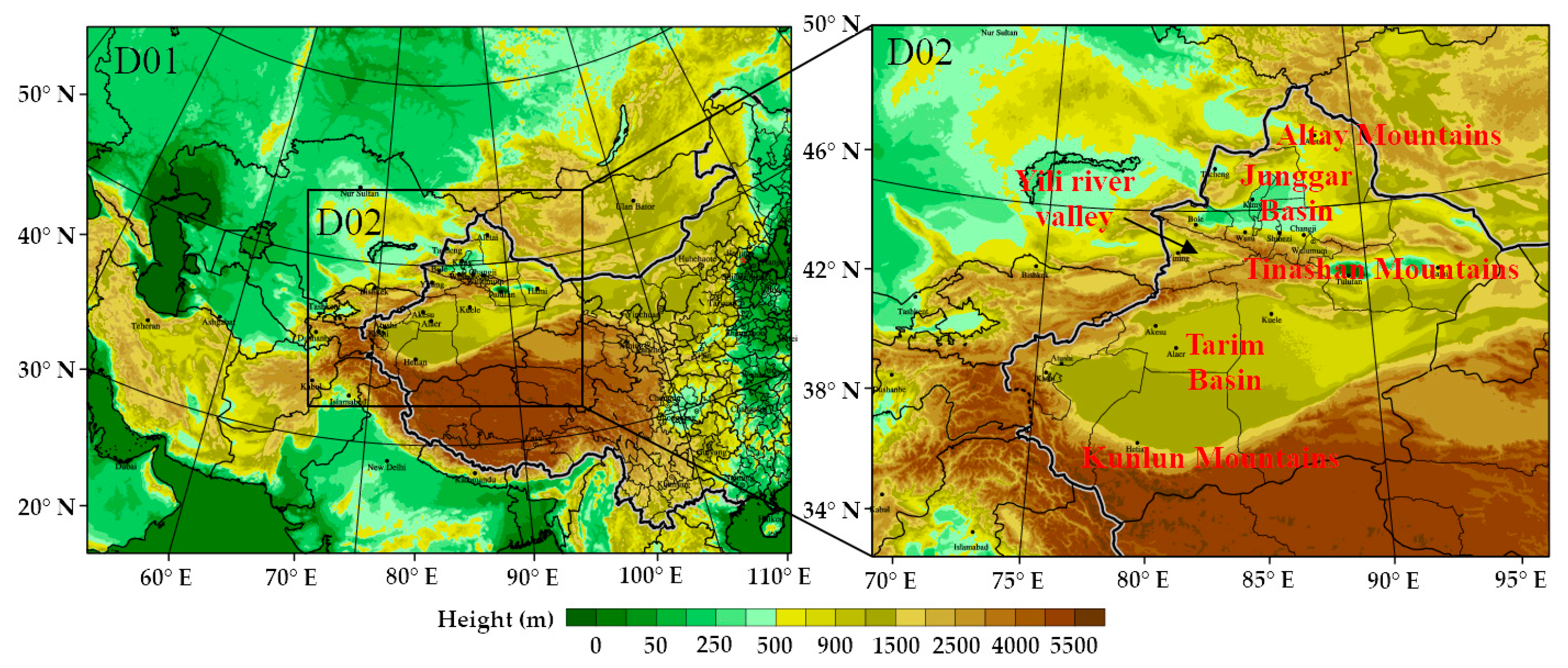
2. Model and Experimental Design

2.1. WRF Model

The model used in this study is version 4.1.3 of WRF, which was recently developed from the ongoing Mesoscale Model (MM5). The fully compressible conservative form of the non-hydrostatic atmospheric model is designed for both research and operational numerical weather prediction (NWP) applications. The WRF is suitable for various applications across scales ranging from meters to thousands of kilometers. The WRF is a fully compressible non-hydrostatic model with a horizontal lattice in Arakawa-C format, a hybrid vertical coordinate system of power quality, and a Euler center-based on-terrain following. Physical parameterization schemes can be selected in the model, including microphysics, cumulus, planetary boundary layer, and land surface processes. The WRF modeling system includes the WRF Pre-Processing System (WPS), the Advanced Research WRF (ARW), the WRF data assimilation (WRFDA) and post-processing systems. The WPS contains the initial data used to define the simulation domain, interpolate terrestrial data (including ground vegetation, terrain, soil type, and land use), and horizontally interpolate the initial data into the simulation domains [18,19,20,21].

2.2. Noah and Noah-MP Land Surface Schemes

The Noah land surface model, adopted by WRF, is jointly developed by NCAR and NCEP [22,23,24]. The Noah scheme regards the soil surface layer and vegetation as a whole. The Penman potential evaporation method calculates the latent heat flux [25]; it includes four soil layers with thicknesses of 0.1, 0.3, 0.6, and 1.0 m [26]. The model consists of two equations of soil heat and water vapor conduction. The commonly used heat diffusion equation and the Richards equation calculated soil moisture and water contents. It uses the Reynolds number method to determine the ratio of thermal roughness to momentum roughness [27,28]. Calculating the canopy impedance considers the adequate soil moisture and atmospheric conditions (i.e., the Jarvis plan) at the same time; the Noah model also adds the surface runoff scheme [29].

The Noah-MP is based on the Noah land surface model (V3.0), which separates vegetation from the surface. It adjusts the overall framework of the model [30,31] and extends the options of 10 land surface processes [32,33]. Noah-MP follows most of the Noah model. However, because the Noah-MP land surface process plan separates vegetation from the ground surface, its calculation of soil thermal conductivity removes the relationship between soil thermal conductivity and the reduction of vegetation coverage. The Noah-MP scheme mainly enhances the characterization capabilities of vegetation ecology, snow treatment, and groundwater processes. Each sub-physical process has 2~4 parallel physical options which can be flexibly selected for the target area [29,34,35,36].

In this paper, the parameterization scheme of the sub-physical quantity process in Noah-MP LSS used the default options: using the table to assign the value of leaf area index assignment, maximum vegetation coverage, the Ball-Berry canopy impedance scheme [37], the Monin-Obukhov surface exchange coefficient calculation scheme [38], the soil moisture control factor related to the canopy impedance in the Noah model [33], the TOPMODEL runoff scheme [39], linear soil permeability scheme [40], the two-stream radiation transmission scheme using vegetation coverage, treatment of supercooling water in frozen soil [40], and the CLASS snow cover surface albedo scheme [41].

2.3. Numerical Simulation Setups

Comparative simulations were performed using WRF 4.1.3. The background field and boundary conditions used the GFS (Global Forecast System) 0.5° × 0.5° data of NCEP (National Centers for Environment Prediction). The simulation nested domain and topography are illustrated in Figure 1. It adopts double nesting: domain 1 covers Central Asia, with a horizontal resolution of 9 km; domain 2 covers Xinjiang, with a horizontal resolution of 3 km (Figure 1). The configuration of the parameterization schemes is as follows: the microphysics scheme from the WSM6 [42] and the cumulus scheme from Kain–Fritsch [43] (domain 2 without the cumulus process), the RRTMG scheme for long-wave and short-wave radiations [44,45,46], the planetary boundary layer scheme is the YSU scheme [47], and the LSS is the Noah/Noah-MP scheme [48]. The land cover data was derived from GLC2015 (Global Land Cover 2015), the data developed by Li et al. [14], and the land cover types were divided into 24 categories. The details configurations of the simulations used in WRF are provided in

Table 1. Grids and detailed parameterization schemes of simulation.

	D01	D02
Horizontal resolution	9 km	3 km
Horizontal grid setting	712 × 532	832 × 652
Microphysics	WSM6	WSM6
Cumulus	K-F	--
Planetary boundary layer	YSU	YSU
Long-wave	RRTMG	RRTMG
Short-wave	RRTMG	RRTMG

.

To systematically evaluate the forecast effect of Noah-MP and Noah scheme, the forecast samples used for verification were from 00:00 on 1 January 2017 (UTC, the same below) to 12:00 on 31 January 2017 (represents the winter) and from 00:00 on 1 July 2017 to 12:00 on 31 July 2017 (represents the summer). The cyclic forecast was updated once per day (00:00 UTC), each prediction’s timeliness was 24 h, and the total number of samples was 62.

2.4. Observational Data and Metrics of the Evaluation

The observational data was from Meteorological Unified Service Interface Community (MUSIC) which the National Meteorological Information Center developed; the data includes surface wind speed, 2-m air temperature, and soil temperature (measured at 5 and 20 cm thickness from 105 national stations), and soil volumetric moisture content. For the soil volumetric moisture measurement, the data was obtained from 40 stations in January 2017, of which 27 were national stations and 13 were regional stations, and from 84 stations in July 2017, of which 62 were national stations and 22 were regional stations. Measurements were done at 0~10 and 20~30 cm thicknesses.

In WRF model, the 2-m temperature is diagnosed by means of [14]:

$$T_{2m}=T_s-\frac{H}{\rho c_p{C}_H}$$

(1)

$$C_H=\frac{k\times u_{\ast }}{ln\left(\frac{2m}{z_{0h}}\right)-{\psi }_H}$$

(2)

where $\rho$ and $c_p$ are the air density and heat capacity of air, respectively, k = 0.4 is the von Karman’s constant, $z_{0h}$ is the roughness length for heat, ${\psi }_H$ is the integrated universal function for heat, and $u_{\ast }$ represents the friction velocity at 2 m.

The wind speed can be calculated as follows [14]:

$$U_{\left(Z\right)}=\left(\frac{u_{\ast }}{k}\right)ln\left(\frac{Z}{Z_{0m}}\right)$$

(3)

In Equation (3), $U_{\left(Z\right)}$ is the horizontal wind velocity at height z above the grounyou, $u_{\ast }$ is the frictional velocity, and $k$ is the von Kalman constant, which has a value of 0.4 in this work.

The hourly observation data of soil surface heat flux was observed at the Institute of Desert Meteorology (IDM), the data were obtained at two stations (Hongliuhe and Kelameili) in January 2017 and two stations (Hongliuhe and Xiaotang) in July 2017; measurements were done at 5 cm thickness. The observation time of Hongliuhe station was from 1:00 a.m. to 6:00 a.m. and 5:00 p.m. to 12:00 a.m. (UTC, the same below), and the observation time of Xiaotang and Kelameili stations was from 1:00 a.m. to 12:00 a.m. Soil heat flux refers to the heat passing through a unit area of soil per unit time, which is calculated as [14]:

$$G=-{\lambda }_s\frac{\partial T}{\partial z}$$

(4)

where G and z are soil heat flux (unit: W·m⁻²) and soil thickness (unit: m), respectively (both downward are positive), and T is soil temperature (unit: K), λ is soil thermal conductivity (unit: W/mK).

Since WRF/Noah and WRF/Noah-MP include four-layer soil models, the thicknesses are 0.1, 0.3, 0.6, and 1 m, i.e., the effective depth of each thickness is 5, 25, 75, and 150 cm, respectively [26]. Therefore, in this paper, the soil temperature of the first and second layer outputted by WRF compared with the observed soil temperature values at 5 and 25 cm thickness. Hence, the simulated values of the soil water content of the first layer (5 cm) and the second layer (25 cm) were compared with the observed values of 0~10, and 20~30 cm, respectively, and the simulated values of the surface soil heat flux were compared with the observed values of 5 cm thickness.

The statistical evaluations used in this study were the mean error (ME), which is calculated as [15]:

$$ME=\frac{1}{N}\left[{\displaystyle \sum }_{i=1}^N\left(F_i-O_i\right)\right]$$

(5)

and the root mean squared error (RMSE), which is calculated as [15]:

$$RMSE=\sqrt{\frac{1}{N}{\displaystyle \sum }_{i=1}^N{\left(F_i-O_i\right)}^2}$$

(6)

where F_i is the forecast value at time i and O_i is the observed value at time i. The comparison of the forecasting performance of Noah-MP and Noah scheme in January and July is useful to improve the understanding of the forecasting performance of the two LSSs in Xinjiang arid region.

3. Comparison Simulation Results

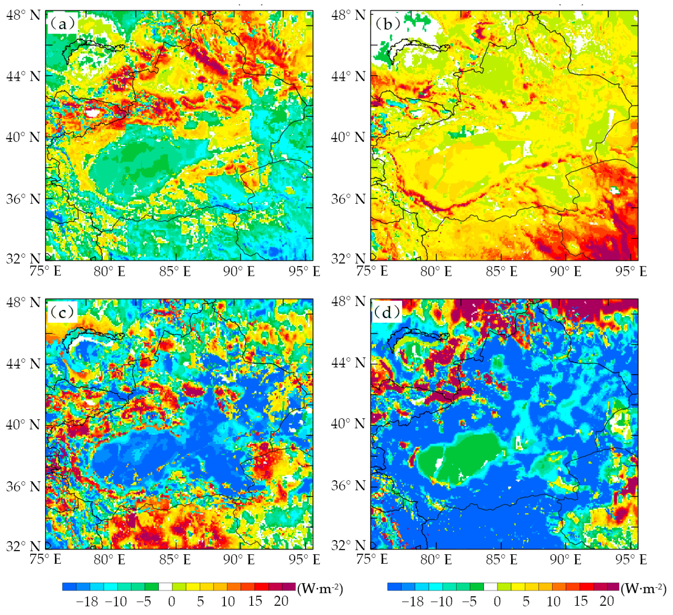
3.1. Surface Flux

Land surfaces with various underlying surfaces exchange momentum, water vapor, and energy with the atmosphere through sensible heat flux and latent heat flux distribution. Figure 2 shows the monthly mean differences between Noah and Noah-MP (Noah–Noah-MP) for surface flux simulation in January and July 2017. In January, the surface sensible heat flux simulated by the Noah-MP scheme was slightly higher (than the Noah scheme) in the Taklimakan Desert and the Gobi region of eastern Xinjiang, whereas, the northern Xinjiang region simulation was relatively low (15~20 W·m⁻²), especially in the Tianshan Mountains and Altay Mountains. The Noah LSS treats the surface soil and canopy as a whole, including snow, leading to a large amount of energy stored on thick snow surfaces [32]. Thus, Noah’s sensible heat flux in northern Xinjiang simulated in January was large. The Noah-MP scheme separates the surface and vegetation layers and increases the snow cover to three layers. Thus, the sensible heat flux is reduced [27,36]. At the same time, it has been proven that the Noah scheme uses the Reynolds number method to determine the ratio of thermal roughness to momentum roughness, which overestimates the sensible heat flux when the vegetation height is low [48,49]. Compared to Noah, except for some areas in the northern mountainous region of southern Xinjiang, the surface latent heat flux simulated by Noah-MP was relatively low in most regions of Xinjiang. However, there was generally ≤10 W·m⁻²; only lower than 12 W·m⁻² in the southern mountainous areas of the south Xinjiang.

In July, compared to Noah, Noah-MP produced a lower sensible heat flux value in most areas of northern Xinjiang and the mountainous regions of southern Xinjiang (≤ 20 W·m⁻²), but the simulated surface heat flux in the Xinjiang basin and desert areas was overestimated (15~20 W·m⁻²). This observation could be attributed to different surface heat exchange coefficients between the two LSSs, as Noah-MP considers the influence of zero plane displacement [11]; therefore, the difference was evident in areas with high vegetation coverage in summer. Comparing the surface latent heat flux in July, the simulated values of Noah-MP for most parts of Xinjiang were higher than Noah’s (15~20 W·m⁻²), except for the western Tianshan Mountains and the northern Altay Mountains (≥18 W·m⁻²). The main reason for the discrepancy may be that the Ball-Berry canopy impedance scheme adopted in Noah-MP was more conducive (than Noah scheme) to vegetation transpiration under vegetation growth conditions in summer.

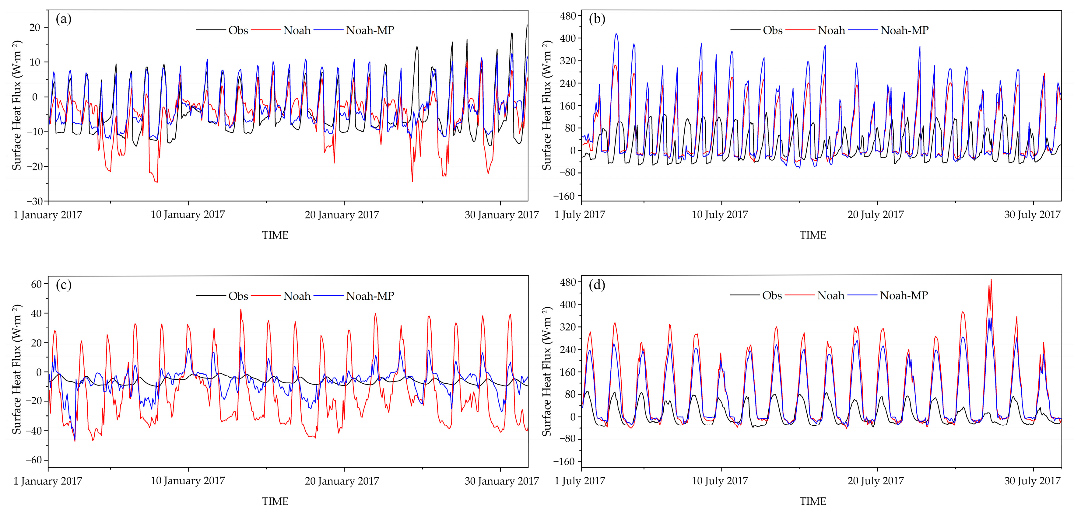
3.2. Surface Soil Heat Flux Simulation at Observation Stations

Figure 3 shows the simulated surface soil heat flux of three stations between the two LSSs, and it can be seen that Noah-MP significantly reduced the negative deviation compared to Noah, because they use different parameterization schemes for surface soil thermal conductivity [47]. The evaluation metrics of the surface soil heat flux at 5 cm thickness are shown in

Table 2. ME and RMSE of simulated surface soil heat flux at 5 cm thickness in WRF simulations with Noah and Noah-MP scheme in January and July 2017 (unit: W·m⁻²).

Metrics/Station/Scheme	January				July
	Hongliuhe		Kelameili		Hongliuhe		Xiaotang
	ME	RMSE	ME	RMSE	ME	RMSE	ME	RMSE
Noah	−0.97	7.34	−7.47	25.61	45.81	77.34	87.75	131.47
Noah-MP	1.14	4.08	−1.44	9.80	62.62	104.50	71.01	104.49
Δ	−17.5%	44.4%	80.7%	61.7%	−36.7%	−35.1%	19.1%	20.5%

(Δ presents the ratio of improvement, Δ = −100%(|Noah-MP| − |Noah|)/|Noah|, the same blow) in January; compared to Noah, Noah-MP simulated surface soil heat flux at Honglihe and Kelameili stations were closer to the observations, the ME of surface soil heat flux increased by 17.5% and reduced by 80.7%, respectively, and the RMSE of surface soil heat flux reduced by 44.4% and 61.7%, respectively. In July, compared to Noah, Noah-MP scheme’s simulated surface soil heat flux at Honglihe station was more deviated from the observations but was closer to the comments at Xiaotang station, the ME of surface soil heat flux increased by 36.7% and reduced by 19.1%, respectively, and the RMSE of surface soil heat flux increased by 35.1% and reduced 20.5%, respectively. Compared to Noah, Noah-MP simulated the surface soil heat flux better for Hongliuhe and Kelameili stations in January, and better for Xiaotang stations in July. In conclusion, station verification results show that Noah-MP simulates the soil heat flux better than Noah over the arid regions in Xinjiang.

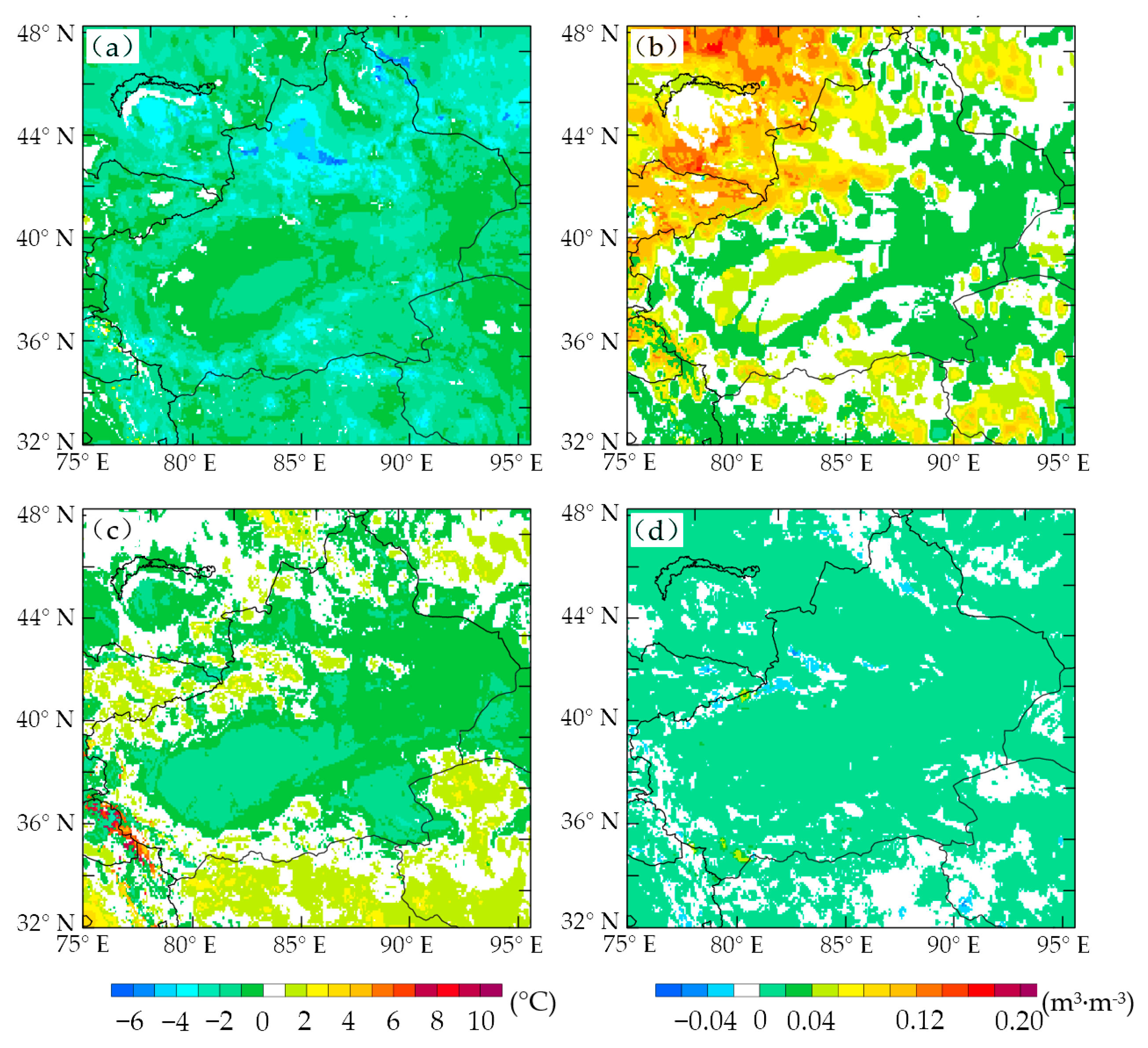
3.3. Simulation of Soil Temperature and Moisture

Studies have shown that surface cover and soil characteristics (surface temperature, soil temperature, humidity, etc.) directly influence the distribution of sensible and latent heat fluxes under different underlying surface conditions. Also, these factors determine whether LSSs can accurately simulate soil temperature and soil moisture directly, which in turn affects the simulation of sensible surface heat and latent heat flux [50]. Figure 4 shows the difference in surface soil temperature and humidity simulation between the two schemes.

In January, Noah-MP simulated a higher surface soil temperature (at 5 cm thickness) than Noah in almost the entire Xinjiang region (≤4 °C), especially in the Yili river valley, the west Tianshan mountains, and the northern mountains of Altay (5~7 °C). For the first layer of soil moisture, except for the mountainous areas along the southern and eastern Xinjiang, Noah-MP simulation for most areas was low (≤0.06 m³·m⁻³), especially in the Yili river valley and west Tianshan mountains (0.08~0.14 m³·m⁻³). It should be noted that the Noah treats the surface soil and canopy as a whole. When the snow is thicker, a large amount of energy is stored on the snow surface, and the snow melts quickly, which reduces the surface temperature. Hence, the corresponding surface soil temperature is also relatively low. At the same time, the penetration of snow water into the soil causes the surface soil moisture to increase accordingly [40]. However, Noah-MP addresses the above problems by separating the canopy layer from the ground surface layer, adding up to three layers of snow patterns, and increasing the permeability of frozen soil [39].

In July, compared to Noah, Noah-MP scheme’s simulated surface soil temperature was lower in the central Tianshan mountains and western mountainous areas of southern Xinjiang (2~4 °C) but higher in other Xinjiang areas (≤3 °C). Also, the simulation of surface soil moisture in the Noah-MP scheme was somewhat indifferent to Noah, and the overall simulation was relatively dry but slightly wet in some mountainous areas of Xinjiang. Overall, the simulation difference in July was smaller than in January, mainly reflected by the difference in the treatment of frozen soil and snow cover between the Noah-MP and Noah schemes, resulting in the significant changes in the simulation of surface temperature and humidity in winter. The difference in canopy impedance and surface exchange coefficient had little effect under uniform vegetation conditions in summer.

Figure 5 shows the monthly ME of the surface and the second layers soil temperature simulated by Noah and the Noah-MP scheme in January 2017. We observed that the soil temperature simulated by the WRF model using two schemes was high primarily in Xinjiang, except for the first layer soil temperature of the northern Xinjiang. Except for the first layer soil temperature simulation, the simulation deviation of Noah in the north Xinjiang region in January was greater than that of Noah-MP, but the difference in simulation was not huge. The overall performance of the soil temperature simulation of the two schemes in July was the cold deviation in northern Xinjiang and the warm deviation in southern Xinjiang. In July, the simulated cold and warm deviations (in July) were more significant than in January (Figure omitted). The effect of soil temperature simulated by Noah-MP scheme in WRF ensued during winter in northern Xinjiang. The evaluation metrics of the soil temperature at 10 cm and 30 cm thickness are shown in

Table 3. ME and RMSE of the simulated soil temperature at 10 cm and 30 cm thickness in WRF simulations with Noah and Noah-MP schemes in January and July 2017 (unit: °C).

Metrics/Scheme	January				July
	ME		RMSE		ME		RMSE
	10 cm	30 cm	10 cm	30 cm	10 cm	30 cm	10 cm	30 cm
Noah	−1.87	1.19	5.06	3.08	−0.28	−0.93	9.71	5.03
Noah-MP	−0.28	1.24	4.38	2.90	0.06	−0.39	10.31	4.91
Δ	85.0%	−4.2%	13.4%	5.8%	78.6%	58.1%	−6.2%	2.4%

, and the results demonstrated that Noah-MP significantly reduced the overestimation of soil temperature. In January, compared to Noah, the ME of the soil temperature at 10 cm and 30 cm thickness simulated by Noah-MP reduced by 85.0% and increased by 4.2%, respectively. The RMSE of soil temperature reduced by 13.4% and 5.8%, respectively. In July, compared to Noah, the ME of soil temperature simulated by Noah-MP reduced by 78.6% and 58.1%, respectively, and the RMSE of soil temperature increased by 6.2% and reduced by 2.4%, respectively. This indicates that the effects of Noah-MP alleviate the surface and the second soil temperature underestimation.

Furthermore, Figure 6 depicts the monthly ME of the surface soil moisture and that simulated by the Noah and Noah-MP schemes in January 2017. The bias of the simulated value was generally high for the two schemes, except for several stations on the south side of the west Tianshan Mountains. However, the Noah-MP scheme exhibited reduced surface soil moisture overestimation at the northern Xinjiang stations, accompanied by a latent underestimation. Moreover, little difference existed between the two schemes simulated bias for the second soil moisture layer in January 2017. At the same time, the two LSSs had little difference in soil moisture bias in July (Figure omitted).

To further analyze the simulation ability of Noah and the Noah-MP scheme in Xinjiang, we assessed the difference in monthly mean RMSE (RMSE_Noah-RMSE_Noah-mp, the same below) of soil moisture simulated by the Noah and Noah-MP schemes (Figure 7). We observed that Noah-MP’s simulations were superior to Noah’s, especially for the Yili river valley and the north side of the Tianshan Mountains. The Noah uses a relatively simple, free drainage plan [32,51], while the Noah-MP calculates the surface runoff and groundwater based on the TOPMODEL flow model [40]. The runoff scheme adopted by the Noah-MP model considers the exchange between the unconfined water layer and upper soil and the influence of groundwater flow on the soil moisture [2,39], which improves the calculation. This property makes the simulation effect of soil moisture in the Noah-MP model better than in the Noah model. The evaluation metrics of soil moisture at 10 cm and 30 cm thickness are shown in

Table 4. ME and RMSE of simulated soil moisture at 10 cm and 30 cm thickness in WRF simulations with Noah and Noah-MP scheme in January and July 2017 (unit: m³·m⁻³).

Metrics/Scheme	January				July
	ME		RMSE		ME		RMSE
	10 cm	30 cm	10 cm	30 cm	10 cm	30 cm	10 cm	30 cm
Noah	0.125	0.089	0.161	0128	0.003	0.007	0.109	0.109
Noah-MP	0.041	0.069	0.137	0.131	0.002	0.007	0.106	0.109
Δ	67.2%	22.4%	14.9%	−2.3%	33.3%	--	2.8%	--

, and the results demonstrated that Noah-MP significantly reduced the overestimation of soil moisture. In January, compared to Noah, the ME of soil moisture at 10 cm and 30 cm thickness simulated by Noah-MP reduced by 67.2% and 22.4%, respectively, the RMSE of soil moisture reduced by 14.9% and increased by 2.3%, respectively. In July, compared to Noah, the ME and RMSE of soil moisture at 10 cm thickness simulated by Noah-MP reduced by 33.3% and 2.8%, respectively. This indicates that the effects of Noah-MP alleviate the surface soil moisture overestimations.

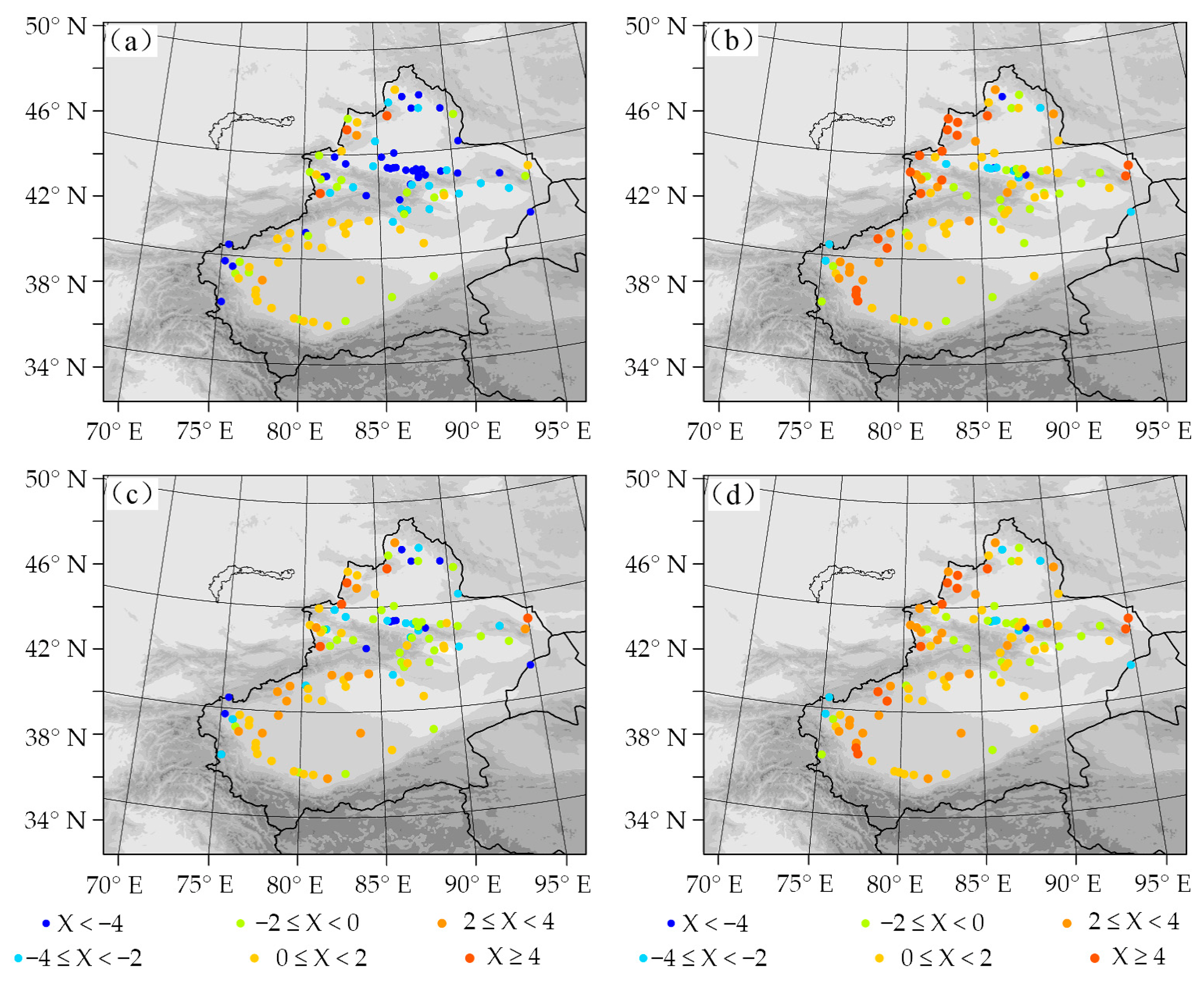
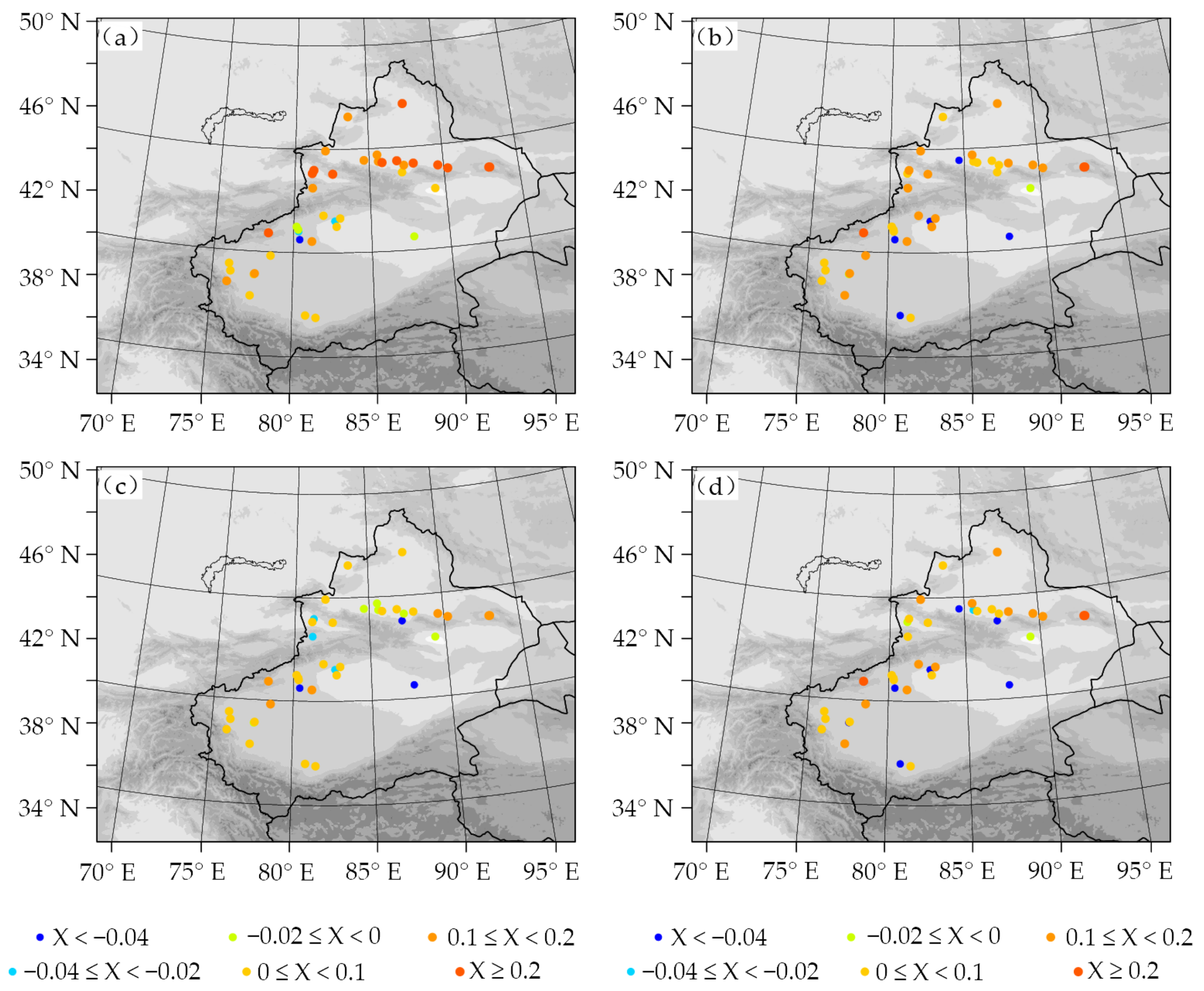
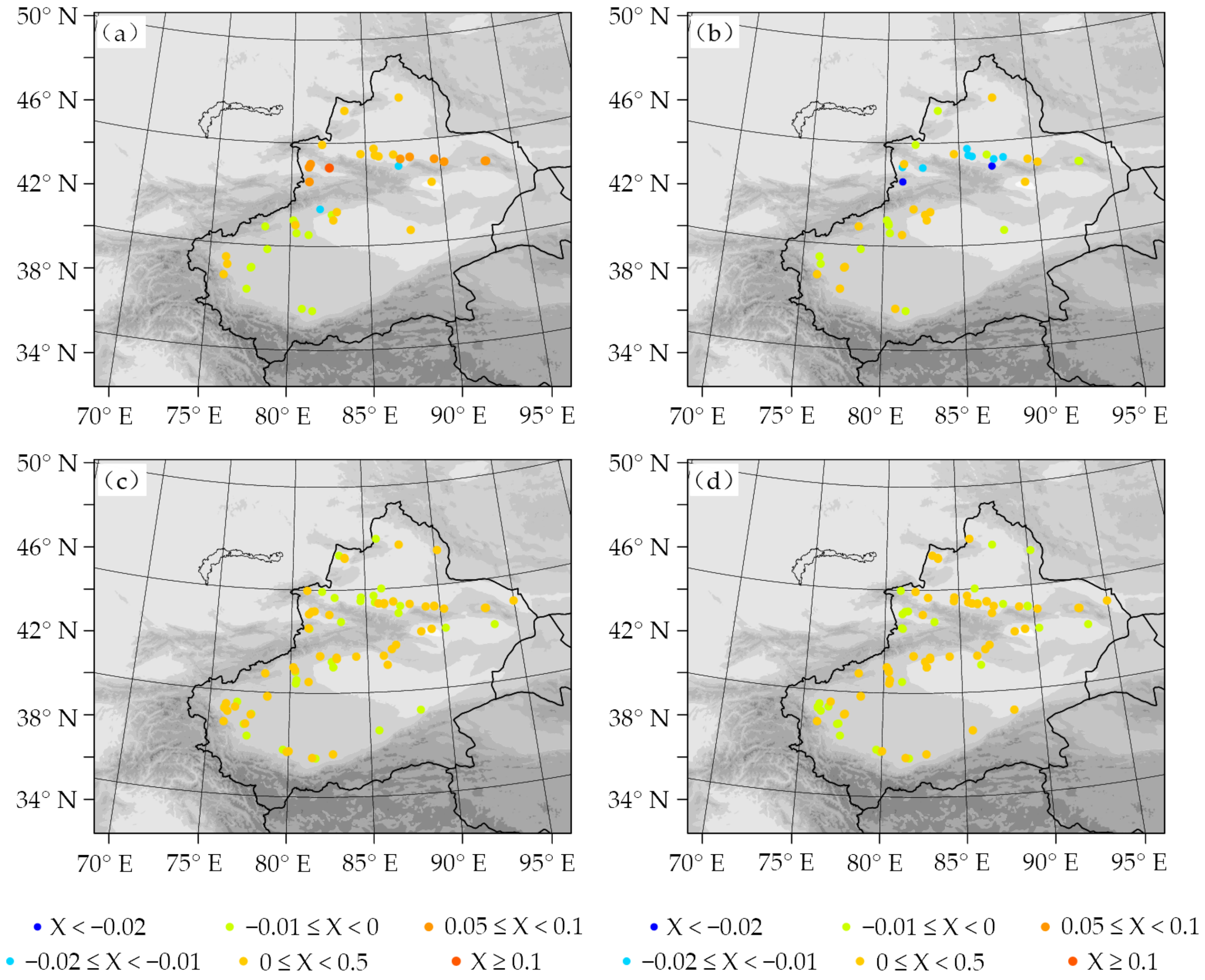
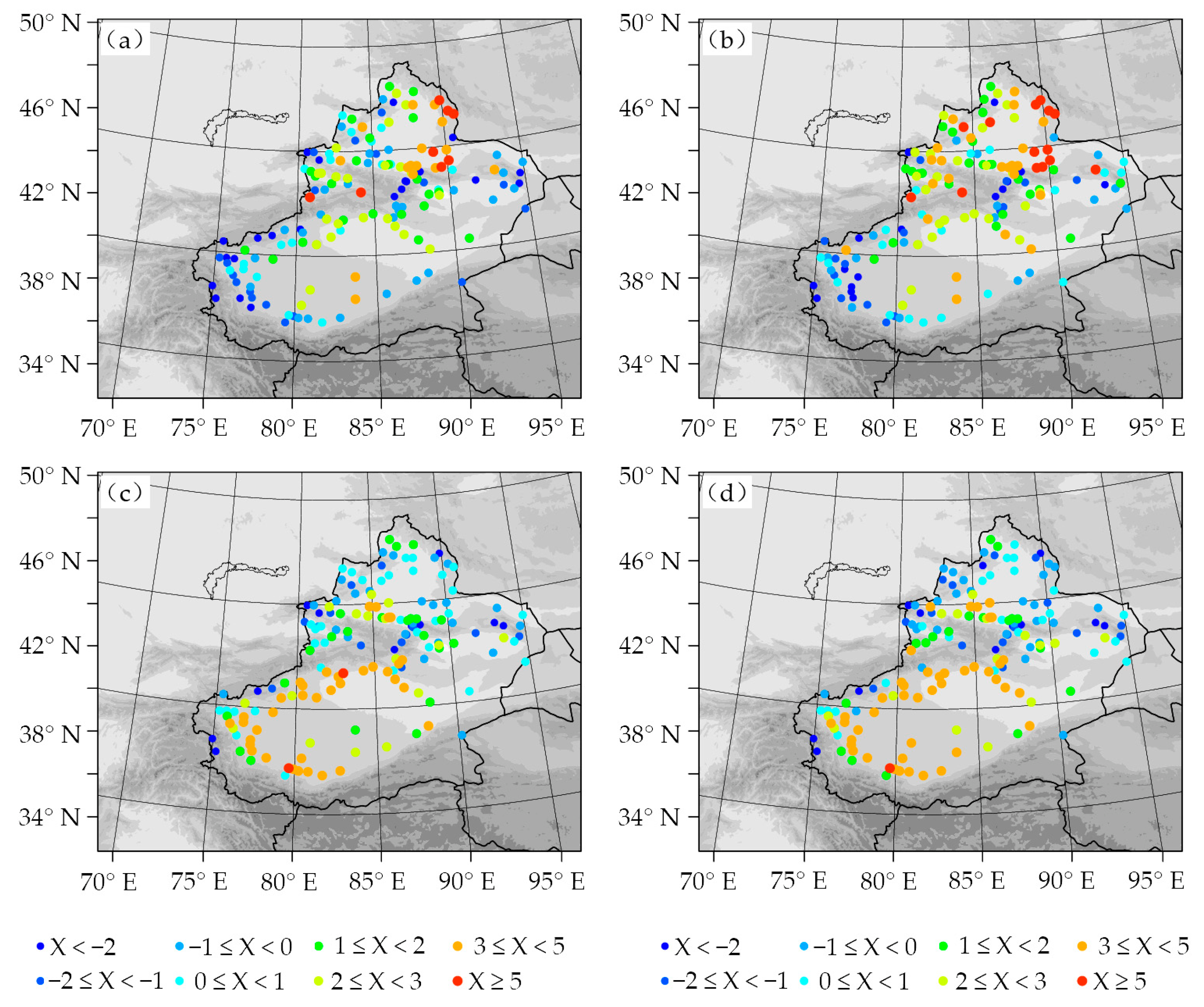
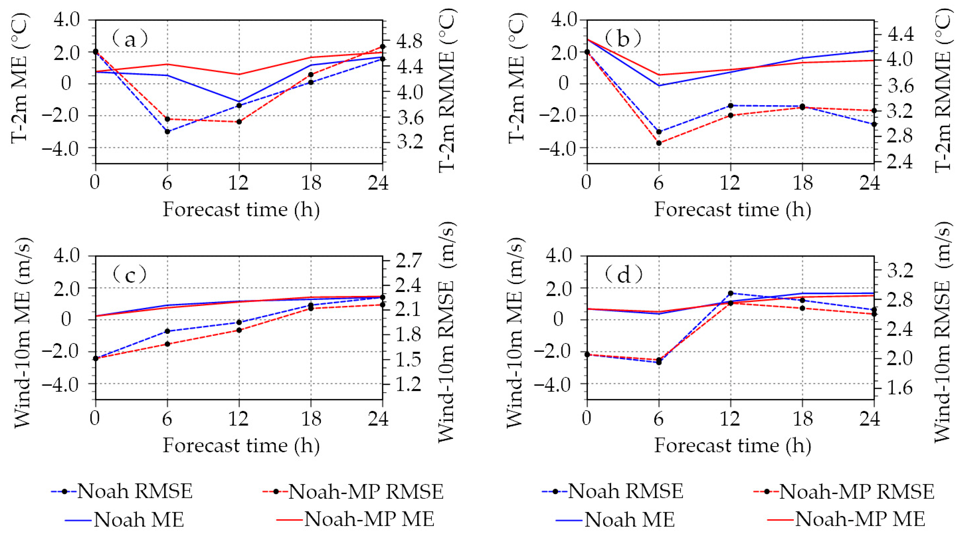
3.4. Near-Surface Variables

The 2-m air temperature, mixing ratio, and 10-m wind speed output by WRF are examined through surface temperature, surface humidity, sensible heat flux, and latent heat flux. Thus, changes in surface energy balance, soil temperature, and moisture (Figure 2 and Figure 4) would affect these surface diagnostics.

Figure 8 illustrates the ME of 2-m temperature monthly simulated by the Noah and Noah-MP schemes; 157 stations contributed to the near-surface variables. In January, the 2-m temperature bias simulated by the two LSSs showed a warm deviation in the north of the Tianshan Mountains and a cold deviation in the south of the Tianshan Mountains. However, in July, the bias showed a cold deviation in the north of the Tianshan Mountains and a warm deviation in the south of the Tianshan Mountains. In the Noah scheme, the treatment of frozen soil makes its permeability poor, resulting in an increase in surface runoff in spring or early summer, and a decrease in snow water penetrating the soil [40]. To solve the above problems, Noah-MP separates the canopy from the surface layer, adds up to three layers of snow mode, and increases the permeability of the frozen soil [39]. Therefore, Noah-MP had an excellent simulation effect on soil temperature, soil moisture, and corresponding 2-m air temperature in winter north and east of the Tianshan Mountains.

In addition, Section 3.1 reveals that, in winter, the sensible heat flux and latent heat flux which Noah-MP simulated was lower (compared to Noah scheme) in most areas of northern Xinjiang. Whereas in summer, the simulation of sensible heat flux of the Noah-MP scheme in the north of Xinjiang was relatively low, while that of latent heat flux was high in most areas. For a specific underlying surface, the reduction of surface heat flux transmitted to the atmosphere means lowering heat exchange between the surface and the atmosphere and vice versa. Therefore, in the winter of 2017, the Noah-MP scheme evinced a reduced positive deviation of the 2-m temperature in northern and eastern Xinjiang. Similarly, in the summer of 2017, the positive deviation on the southern slope of the Tianshan Mountains was reduced (Figure 8).

To better investigate the impact of the two LSSs on the simulation of near-surface variables, Figure 9 depicts the differences of the monthly RMSE (RMSE_Noah-RMSE_Noah-mp) of 2-m air temperature and 10-m wind speed simulations. In January, compared to Noah, the RMSE of 2-m temperature simulated by Noah-MP was lower (≤2 °C) in southern Xinjiang but slightly higher (at 0~1 °C) in northern Xinjiang. In July, compared to Noah, the RMSE of 2-m temperature simulated by Noah-MP was generally higher in southern Xinjiang but lower in northern Xinjiang, within ±1 °C. For 2-m air temperature, the difference of the monthly mean RMSE between the two LSSs was >2 m·s⁻¹ in winter and −1~1 m·s⁻¹ in summer. Generally, Noah-MP showed little difference from Noah and performed better in some stations in northern Xinjiang during winter. The evaluation metrics of 2-m air temperature and 10-m wind speed are shown in

Table 5. ME and RMSE of simulated 2-m temperature (unit: °C) and 10-m wind speed (unit: m·s⁻¹) with Noah and Noah-MP scheme in January and July 2017.

Metrics/Scheme	January				July
	ME		RMSE		ME		RMSE
	T2m	Wind10m	T2m	Wind10m	T2m	Wind10m	T2m	Wind10m
Noah	0.57	1.20	3.95	2.05	1.09	1.21	3.10	2.57
Noah-MP	1.37	1.19	4.02	1.95	1.06	1.13	3.07	2.50
Δ	−140%	0.8%	−0.18%	4.9%	2.8%	6.7%	1.0%	2.8%

, and the results demonstrated that Noah-MP significantly reduced the overestimation of 10-m wind speed in winter and 2-m air temperature, 10-m wind speed in summer. Compared to Noah, Noah-MP significantly reduced the overestimation of near-surface variables. In January, the ME and RMSE of 10-m wind speed simulated by Noah-MP reduced by 0.8% and 4.9%, respectively. In July, the ME of 2-m air temperature and 10-m wind speed reduced by 2.8% and 6.7%, respectively, and the RMSE reduced by 1.0% and 2.8%, respectively. This indicates that the effects of Noah-MP alleviate 2-m air temperature and 10-m wind speed overestimations.

Figure 10 illustrates the daily cycle variation of regional ME and RMSE of 2-m air temperature and 10-m wind speed. For 2-m temperature simulation, compared to Noah, the ME and RMSE of 2-m temperature simulated by Noah-MP was relatively higher than Noah in winter, but both of them were lower than Noah in summer. For the 10-m wind speed simulated by the two LSSs, the ME and RMSE of Noah-MP were relatively lower than Noah in winter and summer, but the overall difference in the ME and RMSE were slight.

4. Summary and Discussion

The Noah LSS is the most widely used in various numerical forecasting operational systems globally. At the same time, the Noah-MP is a new multi-physical process alternative formed based on the Noah scheme. This work conducted whole month numerical simulation experiments in the Xinjiang arid region in January and July 2017 using the Noah and Noah-MP schemes. The evaluation mainly compared WRF output variables to observations stations, including near-surface variables and soil variables, and the conclusions were as follows:

In winter, except for the Taklimakan Desert and the Gobi region of eastern Xinjiang, the surface sensible heat flux simulated by Noah-MP was relatively lower than that of Noah (15~20 W∙m⁻²), especially in the Tianshan Mountains and the Altay Mountains; moreover, Noah-MP-simulated surface latent heat flux was relatively low in most areas of Xinjiang (<10 W∙m⁻²). In summer, Noah-MP mainly had a lower value (than Noah) of the sensible heat flux in most regions of northern Xinjiang and the mountainous areas of southern Xinjiang (≤20 W·m⁻²). Also, the simulated surface heat flux in the Xinjiang basin and desert areas was excessively higher (15~20 W·m⁻²), except for parts of the western Tianshan Mountains and the northern Altay Mountains (≥18 W·m⁻²). Generally, the surface latent heat flux simulated by Noah-MP was higher for most regions of Xinjiang. And for the simulated surface soil heat flux at observation stations, compared to Noah, Noah-MP was closer to the observations at Hongliuhe and Kelameili stations in January and the Xiaotang station in July.

Compared to Noah LSS, Noah-MP calculates surface runoff and groundwater discharge more accurately, dividing the snow and vegetation into multiple-layer treatments. Therefore, in winter, Noah-MP had a better overall simulation of soil moisture and soil temperature in northern Xinjiang and the Yili river valley. Noah-MP alleviated the soil temperature and moisture overestimation according to the mean and the root mean squared error.

The positive deviation of the 2-m temperature in the northern and eastern Xinjiang during the winter of 2017 and the southern slope of the Tianshan Mountains during the summer of 2017, derived by Noah-MP, were reduced. And for the simulation of 10-m wind speed, Noah-MP performed poorly in winter but slightly better in northern Xinjiang in summer. According to the mean error and the root mean squared error, Noah-MP alleviated 2-m air temperature and 10-m wind speed overestimation.

From the time variation of the average regional ME and RMSE, the 2-m air temperature simulated by Noah-MP were relatively high in winter and low in summer. For the 10-m wind speed simulation, the RMSE of Noah-MP was relatively low in winter and summer, but the overall difference in them was slight.

In summary, the application research of the Noah-MP LSS in the arid region of Xinjiang has been rarely carried out. In this paper, we aimed at the batch test evaluation of the whole Xinjiang arid region, with numerous data and workloads, so it had not been evaluated and diagnosed in all aspects. However, the winter simulation results of Noah-MP in high latitude areas of Xinjiang (especially mountain stations) were consistent with the results given by Zhang et al. [11]. Therefore, we expect to delve into all aspects of the assessment and diagnosis in the next step. Future work must further evaluate the Noah-MP scheme’s simulation effect in the arid region, combine it with the hourly soil data in different seasons obtained from the latest observations of the Institute of Desert Meteorology (IDM) in the northern and southern Xinjiang field observation bases, and obtain the optimal sub-process combination of the Noah-MP scheme in different underlying surfaces and different seasons in the Xinjiang arid region.

References

1. Duan, Z.; Zhang, Y.; Zhang, W.; Wang, Y. Application research of four cold regions land surface and hydrological model to Qinghai-Tibet plateau frozen soil region. J. Water Res. Water Eng. 2012, 23, 43–50. (In Chinese) [Google Scholar]
2. Wang, Y.; Zeng, X.; Ge, H.; Zhang, C. Sensitivity simulation of heavy rainfall to land surface characteristics and ensemble forecast test. Meteorol. Mon. 2014, 40, 146–157. [Google Scholar]
3. Wei, J.; Dirmeyer, P.; Guo, Z. How much do different land models matter for climate simulation? Part I: Climatology and variability. J. Clin. 2010, 23, 3135–3145. [Google Scholar] [CrossRef]
4. Henderson-Sellers, A.; Pitman, A.; Love, J. The project for intercomparison of land surface parameterization schemes (pilps): Phases 2 and 3. Bull. Amer. Meteor. Soc. 1995, 76, 489–503. [Google Scholar] [CrossRef] [Green Version]
5. Cao, F.; Dan, L.; Ma, Z. A regional climate coupled model and its influences on climate simulation over East Asia. Chin. J. Atmos. Sci. 2014, 38, 322–336. (In Chinese) [Google Scholar] [CrossRef]
6. Zhou, S.; Luo, Y.; Wang, H. Analysis of occurrence frequency of precipitation feature over Tibetan Plateau, East China and Subtropical North America in Boreal Summer using TRMM data. Meteorol. Mon. 2015, 41, 1–16. (In Chinese) [Google Scholar]
7. Wang, Q.; Yang, M.; Bao, Y.; Yuan, C. Numerical simulation of a high temperature weather process based on different land surface schemes. Meteor. Sci. Tech. 2011, 39, 537–544. (In Chinese) [Google Scholar]
8. Chen, J.; Wang, J. Diurnal cycles of the boundary layer structure simulated by WRF in Beijing. J. Appl. Meteor. Sci. 2006, 17, 403–411. (In Chinese) [Google Scholar]
9. Zhang, Y.; Xiao, A.; Ma, L.; Wang, H.; Ma, Z.; Yuan, Z. Simulation of the “19 June 2010” heavy rainfall event by using WRF coupled with four land surface processes. Meteorol. Mon. 2011, 37, 1060–1069. [Google Scholar]
10. Zhang, G.; Chen, Y.; Li, J. Effects of organic soil in the noah-mp land-surface model on simulated skin and soil temperature profiles and surface energy exchanges for china. Atmos. Res. 2020, 249, 105284. [Google Scholar] [CrossRef]
11. Zhang, G.; Xue, H.; Xu, J.; Chen, J.; He, H. The WRF performance comparison based on noah and noah-mp land surface processes on East Asia. Meteorol. Mon. 2016, 42, 1058–1068. (In Chinese) [Google Scholar]
12. Ju, C.; Li, S.; Yu, X.; Li, M. Simulation of a Heavy Rainfall Case in Xinjiang Using the GRAPES Model with Different Land Surface Schemes. Des. OAS Meteor. 2014, 8, 16–22. (In Chinese) [Google Scholar]
13. Li, H.; Mamtimin, A.; Ju, C. Simulation and Analysis of Land-Surface Processes in the Taklimakan Desert Based on Noah LSM. Adv. Meteor. 2019, 2019, 1750102. [Google Scholar] [CrossRef]
14. Li, M.; Ju, C.; Xin, Y.; Du, J. Evaluation of 24 h precipitation level forecasting of DOGRAFS system during the summer of 2016. Des. OAS Meteor. 2018, 12, 15–21. (In Chinese) [Google Scholar]
15. Ju, C.; Li, M.; Du, J.; Li, H.; Li, H.; Liu, J. The effect of DOGRAFS_3 km on the forecast effect of meteorological elements in Xinjiang during summer. Des. OAS Meteor. 2017, 11, 9–16. (In Chinese) [Google Scholar]
16. Ju, C.; Liu, J.; Du, J.; Li, H.; Li, M. Forecast effect comparison test and evaluation of RMAPS-CA in Xinjiang. Des. OAS Meteor. 2020, 14, 68–77. (In Chinese) [Google Scholar]
17. Ju, C.; Liu, J.; Li, M.; Li, H.; Zhang, H.; Ma, Y.; Mamtimin, A. Objective Verification on RMAPS-CA V2.0 System during 2021. OAS Meteor. 2022, 16, 38–46. (In Chinese) [Google Scholar]
18. Zoltan, T. Ensemble Forecasting in WRF. Bull. Am. Meteor. Soc. 2011, 82, 695–698. [Google Scholar]
19. Skamarock, W.C.; Klemp, J.B. A time-split nonhydrostatic atmospheric model for weather research and forecasting applications. J. Comput. Phys. 2008, 227, 3465–3485. [Google Scholar] [CrossRef]
20. Li, H.; Zhang, H.; Mamtimin, A.; Liu, J. A new land-use dataset for the weather research and forecasting (WRF) model. Atmosphere 2020, 11, 350. [Google Scholar] [CrossRef] [Green Version]
21. Shen, X.S.; Chen, Q.Y.; Sun, J.; Han, W.; Gong, J.D.; Li, Z.C.; Wang, J.J. Development of Operational Global Medium-Range Forecast System in National Meteorological Centre. Meteorol. Mon. 2021, 47, 645–654. [Google Scholar]
22. Pan, H.; Mahrt, L. Interaction between soil hydrology and boundary-Layerdevelopment. Bound-Layer Meteor. 1987, 38, 185–202. [Google Scholar] [CrossRef]
23. Chen, F.; Dudhia, J. Coupling an advanced land surface-hydrology model with the Penn State-NCAR MM5 modeling system. Part II: Preliminary model validation. Mon. Weather Rev. 2001, 129, 587–604. [Google Scholar] [CrossRef]
24. Ek, M.; Mitchell, K.; Lin, Y.; Rogers, E.; Grunmann, P.; Koren, V.; Gayno, G.; Tarpley, J. Implementation of Noah land surface model advances in the National Centers for Environmental Prediction operational mesoscale Eta model. J. Geophys. Res. 2003, 108, 8851. [Google Scholar] [CrossRef]
25. Mahrt, L.; Ek, M. The influence of atmospheric stability on potential evaporation. J. Climate Appl. Meteor. 1984, 43, 170–181. [Google Scholar] [CrossRef] [Green Version]
26. Schaake, J.; Koren, V.; Duan, Q. A simple water balance model (SWB) for estimating runoff at different spatial and temporal scales. J. Geophys. Res. 1996, 101, 7461–7475. [Google Scholar] [CrossRef]
27. Zilitinkevich, S. Non-local turbulent transport: Pollution dispersion aspects of coherent structure of convective flows. In Air Pollution Theory and Simulation; Air Pollution III; Power, H., Moussiopoulos, N., Brebbia, C.A., Eds.; Computational Mechanics Publications: Berlin, Germany, 1995; Volume I, pp. 53–60. [Google Scholar]
28. Chen, F.; Janjic, Z.; Mitchell, K. Impact of atmospheric surface layer parameterization in the new land-surface scheme of the NCEP mesoscale Eta numerical model. Bound Layer Meteor. 1997, 85, 391–421. [Google Scholar] [CrossRef]
29. Chen, F.; Mitchell, K.; Schaake, J.; Xue, Y.; Hua-Lu, P.; Koren, V.; Duan, Q.; Ek, M.; Betts, A. Modeling of land surface evaporation by four schemes and comparison with FIFE observations. J. Geophys. Res. Atmos. 1996, 101, 7251–7268. [Google Scholar] [CrossRef] [Green Version]
30. Liu, X.; Chen, F.; Barlage, M.; Niyogi, D. Implementing dynamic rooting depth for improved simulation of soil moisture and land surface feedbacks in Noah-MP-Crop. J. Adv. Mod. Earth Sys. 2020, 12, e2019MS001786. [Google Scholar] [CrossRef] [Green Version]
31. Liu, X.; Chen, F.; Barlage, M.; Zhou, G.; Niyogi, D. Noah-MP-Crop: Introducing dynamic crop growth in the Noah-MP land surface model. J. Geo. Res. Atmos. 2016, 121, 13953–13972. [Google Scholar] [CrossRef] [Green Version]
32. Niu, G.; Yang, Z.; Mitchell, K.; Chen, F.; EK, M.; Barlage, M.; Kumar, A.; Manning, K.; Niyogi, D.; Roseroe, E. The Community Noah Land Surface Model with Multi-Parameterization Options (Noah-MP): 1. Model Description and Evaluation with Local-scale Measurements. J. Geophys. Res. 2011, 116, D12109. [Google Scholar] [CrossRef] [Green Version]
33. Hong, S.; Yu, X.; Park, S.; Choi, Y.; Myoung, B. Assessing optimal set of implemented physical parameterization schemes in a multi-physics land surface model using genetic algorithm. Geosci. Model Dev. 2014, 7, 2517–2529. [Google Scholar] [CrossRef] [Green Version]
34. Jiang, X.; Niu, G.; Yang, Z. Impacts of vegetation and groundwater dynamics on warm season precipitation over the Central United States. J. Geophys. Res. 2009, 114, D06109. [Google Scholar] [CrossRef]
35. Yang, Z.; Niu, G.; Mithell, K.; Chen, F.; Ek, M.; Barlage, M.; Longuevergne, L.; Manning, K.; Niyogi, D.; Tewari, M.; et al. The Community Noah Land Surface Model with Multi-Parameterization Options (Noah-MP): 2. Evaluation over global river basins. J. Geophys. Res. Atmos. 2011, 116, D12110. [Google Scholar] [CrossRef]
36. Chen, F.; Barlage, M.; Tewari, M. Modeling seasonal snowpack evolution in the complexterrain and forested Colorado Headwaters region: A model inter-comparison study. J. Geophys. Res. 2014, 119, 13795–13819. [Google Scholar] [CrossRef]
37. Ball, J.; Woodrow, I.; Berry, J. A model predicting stomatal conductance and its contribution to the control of photosynthesis under different environmental conditions. In Proceedings of the Progress in Photosynthesis Research: VIIth International Congress on Photosynthesis, Providence, RI, USA, 10–15 August 1986; Volume 4, pp. 221–224. [Google Scholar]
38. Brutsaert, W.A. Evaporation into the Atomsphere; D. Reidel: Dordrecht, The Netherlands, 1982; 229p. [Google Scholar]
39. Niu, G.; Yang, Z.; Dickinson, R. Development of a simple groundwater model for use in climate models and evaluation with Gravity Recovery and Climate Experiment data. J. Geophys. Res. 2007, 112, D07103. [Google Scholar] [CrossRef]
40. Niu, G.; Yang, Z. A simple TOPMODEL-based runoff parameterization (SIMTOP) for use in global climate models. J. Geophys. Res. 2006, 110, D21106. [Google Scholar] [CrossRef] [Green Version]
41. Verseghy, D. GLASS a Canadian land surface scheme for GCMs. I. soil model. Int. J. Climatol. 1991, 11, 111–133. [Google Scholar] [CrossRef]
42. Hong, Y.; Lim, J. The WRF Single-Moment 6-Class Microphysics Scheme (WSM6). J. Korean Meteor. Soc. 2006, 42, 129–151. [Google Scholar]
43. Kain, J. The Kain-Fritsch convective parameterization: An update. J. Appl. Meteor. 2004, 43, 170–181. [Google Scholar] [CrossRef] [Green Version]
44. Clough, S.; Shephard, M.; Mlawer, E. Atmospheric radiative transfer modeling: A summary of the AER codes. J. Quant. Spectrosc. Radiat. Transf. 2005, 91, 233–244. [Google Scholar] [CrossRef]
45. Iacono, M.; Delamere, J.; Mlawer, E.; Shephard, M.; Clough, S.; Collins, W.D. Radiative forcing by long-lived greenhouse gases: Calculations with the AER radiative transfer models. J. Geophys. Res. 2008, 113, D13103. [Google Scholar] [CrossRef]
46. Kramer, M.; Heinzeller, D.; Hartmann, H.; Wim, V.; Stetneveld, G. Assessment of MPAS variable resolution simulations in the grey-zone of convection against WRF model results and observations. Clim. Dyn. 2020, 55, 253–276. [Google Scholar] [CrossRef] [Green Version]
47. Hong, S.; Noh, Y.; Dudhia, J. A new vertical diffusion package with an explicit treatment of entrainment processes. Mon. Weather Rev. 2006, 134, 2318–2341. [Google Scholar] [CrossRef] [Green Version]
48. Chen, F.; Zhang, Y. On the coupling strength between the land surface and the atmosphere: From viewpoint of surface exchange coefficients. Geophys. Res. Lett. 2009, 36, L10404. [Google Scholar] [CrossRef] [Green Version]
49. Zhang, G.; Zhou, G.; Chen, F.; Barlage, M.; Xue, L. A trial to improve surface heat exchange simulation through sensitivity experiments over a desert steppe site. J. Hydrometeor 2014, 15, 664–684. [Google Scholar] [CrossRef]
50. Barlage, M.; Tewari, M.; Chen, F. The effect of groundwater interaction in North American regional climate simulations with WRF/Noah-MP. Clim. Change 2015, 129, 485–498. [Google Scholar] [CrossRef]
51. Achugbu, I.C.; Dudhia, J.; Olufayo, A.A.; Balogun, I.A.; Gbode, I.E. Assessment of WRF Land Surface Model Performance over West Africa. Adv. Meteor. 2020, 51, 6205308. [Google Scholar] [CrossRef]
Figure 1. Two nested domains and topography.
Atmosphere 13 00927 g001
Figure 2. Monthly mean differences (Noah−Noah-MP) of simulated sensible heat flux (a,c) and latent heat flux (b,d) in January (a,b) and July (c,d) 2017 between Noah and Noah-MP scheme (unit: W·m−2).
Atmosphere 13 00927 g002
Figure 3. Daily simulation of surface soil heat flux at Hongliuhe (a,b), Kelameili (c), and Xiaotang (d) stations in January (a,c) and July (b,d) 2017 between Noah (red line) and Noah-MP (blue line) scheme, observation is the black line (unit: W·m−2).
Atmosphere 13 00927 g003
Figure 4. Monthly mean differences of simulated surface soil temperature (a,c) and soil moisture (b,d) in January (a,b) and July (c,d) 2017 between Noah and Noah-MP scheme.
Atmosphere 13 00927 g004
Figure 5. Monthly ME of the simulated soil temperature at 5 cm (a,c) and 25 cm thickness (b,d) in WRF simulations with Noah (a,b) and Noah-MP (c,d) scheme in January 2017 (unit: °C).
Atmosphere 13 00927 g005
Figure 6. Monthly ME of simulated soil moisture at 5 cm (a,c) and 25 cm (b,d) thickness in WRF simulations with Noah (a,b) and Noah-MP (c,d) scheme in January 2017 (unit: m3·m−3).
Atmosphere 13 00927 g006
Figure 7. Differences in monthly mean RMSE (RMSENoah-RMSENoah-mp) of simulated soil moistures at 0~10 cm (a,b) and 10~40 cm (c,d) thickness in WRF simulations with Noah and Noah-MP scheme in January (a,c) and July (b,d) 2017 (unit: m3·m−3).
Atmosphere 13 00927 g007
Figure 8. Monthly ME of simulated 2-m air temperature in January (a,b) and July (c,d) 2017 with Noah (a,c) and Noah-MP scheme (b,d) (unit: °C).
Atmosphere 13 00927 g008
Figure 9. Differences of the monthly mean RMSE (RMSENoah-RMSENoah-mp) of simulated 2-m air temperature ((a,c), unit: °C) and 10-m wind speed ((b,d), unit: m·s−1) between WRF simulations with Noah and Noah-MP scheme in January (a,b) and July (c,d) 2017.
Atmosphere 13 00927 g009
Figure 10. Time series of monthly ME (solid line) and RMSE (dashed line) of simulated near-surface variables with Noah and Noah-MP scheme: 2-m temperature (a,b) and10-m wind speed (c,d) in January (a,c) and July (b,d) 2017.
Atmosphere 13 00927 g010