Abstract
The article investigates some of the available measurements (Terra MODIS satellite data) of the aerosol optical depth (AOD) taken in the Arabian Gulf, a zone traditionally affected by intense sand-related (or even sand-driven) meteorological events. The Principal Component Analysis (PCA) reveals the main subspace of the data. Clustering of the series was performed after selecting the optimal number of groups using 30 different methods, such as the silhouette, gap, Duda, Dunn, Hartigan, Hubert, etc. The AOD regional and temporal tendency detection was completed utilizing an original algorithm based on the dominant cluster found at the previous stage, resulting in the regional time series (RTS) and temporal time series (TTS). It was shown that the spatially-indexed time series (SITS) agglomerates along with the first PC. In contrast, six PCs are responsible for 60.5% of the variance in the case of the temporally-indexed time series (TITS). Both RTS and TTS are stationary in trend and fit the studied data series set well.
1. Introduction
Dust clouds and storms occur worldwide, especially in the Middle East, southwestern United States, northern China, and the Saharan desert. The essential conditions triggering these phenomena are the existence of huge dust or sand sources, little vegetation, strong surface winds, and an unstable atmosphere [1]. Dust particles primarily enter the lower atmosphere through saltation bombardment, which depends on the meteorological conditions near the surface, the soil texture, and particle size [2,3,4,5]. Dust is emitted as hydrophobic particles, relatively ineffective as cloud condensation nuclei. However, during their transport in the atmosphere, due to the interaction with gaseous and particulate air pollutants, their hygroscopicity increases, fortunately enhancing the efficiency of dust removal from the atmosphere through precipitation [6,7]. Haywood et al. [8] indicated that the aerosols cause a strong radiative forcing of climate because of their efficient scattering of solar radiation.
The most abundant aerosol in the atmosphere is dust, composed of oxides (silica, iron oxides), quartz, feldspar, gypsum, and hematite [9]. Ginoux et al. [10] emphasized the anthropogenic and natural dust sources.
Many studies [8,11,12,13] have already investigated and documented a significant variability of the airborne desert dust during the past decades in the Middle East, Africa, central Asia, and South America, and identified Shamal (the north-westerly wind blowing over Syria, Iraq, and the Arabian Gulf) as the significant natural trigger of dust storm activities across the Arabian Peninsula. Shamal transports the dust lifted from Syria and Iraq to the Arabian Gulf and Peninsula [14,15,16,17,18]. Still, Notaro et al. [16] identified increased dust activity over eastern Saudi Arabia around the Ad Dahna Desert, with dust transported from the Iraqi Desert and local sources. Yu et al. [18] concluded that a strong wind speed determines higher dust activity along the coast of the Persian Gulf in north-central Saudi Arabia, and one has to consider this influence when tracing the phenomenon along and across United Arab Emirates territory.
Different scientists analyzed the aerosol optical depth (AOD) distribution in south-eastern Asia and the Middle East in correlation with the seasonal conditions [19,20,21] and to determine the air quality modifications in China, Sahel, South Africa, and South America [22,23,24,25]. They showed that the atmospheric heating rates and the absorption characteristics are linearly dependent, noticing a significant difference between the aerosols in the Indian region and the zones with large deserts and high dunes (such as UAE) contributing to the dust loadings in the atmosphere [26].
Other researchers provided the classification of the aerosol types taking into account different characteristics—fine mode fraction and the aerosol index [27], AOD [4,28,29], refraction index, and Ångström exponent [30,31,32].
The long-term trend of AOD over the Arabian Peninsula, and eastern and southern Asia for 2002–2009, estimated based on AERONET data, was increasing. The same tendency was observed over most tropical oceans [33]. A long-term positive AOD trend over the Arabian Peninsula occurred, with a higher seasonal tendency during spring and summer (periods when the dust is transported) [26].
Multivariate statistical analysis became one of the most utilized tools for extracting the common characteristics of big data sets issued from environmental sciences [34,35,36,37,38]. The spatio-temporal analysis of AOD is mainly performed by Principal Component Analysis (PCA, also named EOF—Empirical Orthogonal Functions), non-negative matrix factorization (NMF), and combined Principal Component Analysis (CPCA). These tools helped capture the aerosol regimes, the factors influencing the AOD’s concentrations, and the trends [20,21,22,23,24,25].
Recent studies on dust-aerosol in the UAE evaluated the regional distribution of this type of aerosol and the dust storms’ intensity [26,39,40,41]. Using AERONET data collected from 2006 to 2015, Abuelgasim and Farahat [26] found an increasing trend of AOD in summer and spring and a 4.32% mean annual variation of the aerosol loading. They estimated a variation of 11.36% of the mean annual Ångström exponent for the study period. The highest concentration of aerosols was found in summer, while from November to March, an increasing tendency was found during 2011–2016.
Other scientists [40,41] studied the frequency of the dust storms for nine years, using hourly data recorded at eight airports in the UAE. The variation of the aerosol radius was presented in [4], based on monthly series collected at 387 points for 15 years.
Despite the investigations performed to determine the aerosol’s characteristics and the effect of meteorological conditions on their loadings and transport in the Arabian Gulf region, many aspects of the aerosol’s properties in the UAE remain to be studied.
The AOD time series varies depending on the data structure, aerosol extinction, and surface reflectance [22,23,24]. Still, here, we shall not analyze the connection between these variables, but the spatial and temporal variation of the AOD series for 178 months. This research continues the attempt to understand the aerosol characteristics in the UAE, aspects that have not been treated in the studies [4,26,40,41].
The main contributions of this research are:
- (1)
- Performing the PCA to extract the principal components that describe the AOD series’ characteristics in time and space;
- (2)
- Group the series in clusters (in spatial and temporal dimensions);
- (3)
- Build the ‘regional time series’ (RTS) and the ‘temporal time series’ (TTS) of the AOD, employing an original algorithm based on the clusters previously determined;
- (4)
- Compare the RTS and TTS of AOD with those of the ‘regional time series’ and ‘temporal time series’ of the aerosol radius (AR) [4] to emphasize the common tendencies.
2. Methods and Data Series
The methods employed at the first stage of our investigations are PCA, also called EOF, and Clustering.
The first one was used to estimate the similarity in terms of linear dependence within the data and eventually to qualify regional/global aspects. The second one was performed to evaluate dissimilarity, the natural tendency of grouping (if present) in data, and identifying aspects and events localized in time and/or space.
PCA is a statistical technique that (linearly) transforms (and deflates) a large set of (possibly correlated) variables into a smaller set of orthogonal uncorrelated variables representing the most significant information of the initial variables set. Initially employed in the study of meteorological series [42], its use became frequent in other fields such as ozone series evaluation [43,44] and isolating aerosols’ sources [23] based on AOD retrieved from satellite data.
The PCA method is shortly described in the following.
Let us consider the matrix X, whose columns are the series recorded at each point. If n is the number of series (367, in this case), and m is the number of time units (178 months, here), X is an m × n matrix. It was shown that X can be written as a product of two matrices, Y (m × m) and Z (m × n), of orthogonal functions of position and time.
The equation X = YZ is equivalent to
so, the vector of the values recorded at a certain point is a linear combination of the Y columns (with different weights), under orthogonality conditions.
Formula (1) is called the PCA analysis.
For a symmetric matrix,
there is a decomposition such as
where Λ is the diagonal matrix formed by A’s eigenvalues. Therefore, from (1) and (3) it results that
because Z = YTX.
A = XXT = YZZTYT
A = YΛYT
The j-th eigenvector has a contribution of to X, where are the eigenvalues [25].
When a small dominant set of principal components exists, the technique detects the common characteristics of the data samples and reveals the regional or temporal aspects. The absence of dominant principal components results in the data series independence, so the phenomenon is localized [45].
Modifications of PCA have been proposed, such as sPCA [46] (that proposes sparse loadings), CPCA [47] (to investigate the pattern of a specific element), Common PCA (to simultaneous reduce the dimensionality in different groups) [48], or Combined PCA (to compare the modes in the AOD decomposition) [23,24,49]. PCA was chosen here because we are interested in the common characteristics of the series.
To determine the number of principal components, the scree plot, the Kaiser criterion, and the proportion of the variance explained by each component may be utilized [50,51,52]. Here we employed the combined scree plot and variance explained by each component.
Clustering is a method for identifying patterns and similarities within the data and the natural grouping tendency of the similar objects within a data set of interest.
Different scientists introduced various tests for detecting the optimal number of clusters. Although some are more commonly used (because they are well-known or easier to compute), there is no reason to give more credit to one or another, mainly because they rely on different mathematical and computational techniques. Therefore, the strategy for establishing the optimal number of clusters was a multi-criteria decision obeying the majority rule after performing 30 different tests, including silhouette [53], gap, Duda, Dunn, Hartigan, Hubert, and so on [54]. For example, if 15 tests voted for two clusters, eight for three, five for four, and the rest for six, the chosen number is two. This approach assures choosing the number of clusters with the highest probability among the possible number of such groups. In the previous example, the probability associated with two clusters is 15/30 = 1/2, compared to 4/15, 1/6, and 1/15, associated with other choices.
Agglomerative Hierarchical Clustering has been performed using the R software.
The agglomerative coefficient was computed to determine the grouping quality. The higher this coefficient is, the best the clustering is. The dendrogram showing the elements in each cluster was also plotted.
The regional time series (RTS) (temporal time series (TTS)) was built using the spatially-indexed time series (SITS) (temporally-indexed time series (TITS)) and the following algorithm, which is a modified version of Method II [4] based on the resulting clusters.
Given k data series each containing n values, consecutively recorded at the same time, denote by Y = (yji) (j = 1, …, n, i = 1, …, k) the matrix whose column i is formed by the elements of the i-th series (i = 1, …, k). The steps of the algorithm for determining the representative series are:
- (I)
- Choose the number of clusters, m, and perform the series’ clustering, based on a selection algorithm. Here, the choice is made using 30 criteria presented in [54] and the majority principle: m is the number resulting from the highest number of algorithms.
- (II)
- Among the m clusters computed at step (I), choose the one containing the highest number of series (N) and construct a new matrix, Y1, with the series in this cluster.
- (III)
- Select the representative value in the j-th line of the matrix Y1 to be the average of the values in line j.
- (IV)
- Evaluate the error by using the Mean Standard and Mean Absolute Errors (MSE and MAE) corresponding to all the observation sites.
- (V)
- Plot the resulted series.
The novelty of the approach proposed here consists of the following.
- While selection of the number of clusters in the initial algorithm was left to the user, in this article, an efficient selection procedure is employed.
- If, in the second step, two clusterings are providing the same maximum number of elements in one of the sets, the chosen one is that which maximizes the distances between the clusters and minimizes those inside the groups.
- If, after applying the second criterion, there are two clusters with the same number of elements, the computation is performed with each of them. The best result (that gives the minimum mean average error—MAE, mean standard error—MSE, and mean absolute percentage error (%)—MAPE) is reported.
The trend and level stationarity of RTS and TTS has been checked using the KPSS test [55]. The null hypothesis, H0, was the series stationarity in level (trend), and the alternative one, H1, was the series nonstationarity in level (trend).
Remember that a time series is stationary if the statistical properties of the process generating it remain unchanged over time. Therefore, the mean, variance, and autocorrelation structure are constant over time.
One of the common causes of the violation of H0 is the existence of a trend in the mean due to the presence of a unit root or the existence of a deterministic trend. In the first case, the stochastic shocks have persistent effects. In contrast, in the second one, they have only transitory effects after which the variable tends toward a deterministically evolving (non-constant) mean (and the process is called a trend-stationary).
The KPSS test is based on the time series decomposition into a deterministic trend, a random walk, and a stationary error. In the case of stationarity, the series has a fixed element as intercept, or the series is stationary around a fixed level.
The test was performed at the level of significance of 0.05. If the p-value is less than 0.05, the null hypothesis is rejected.
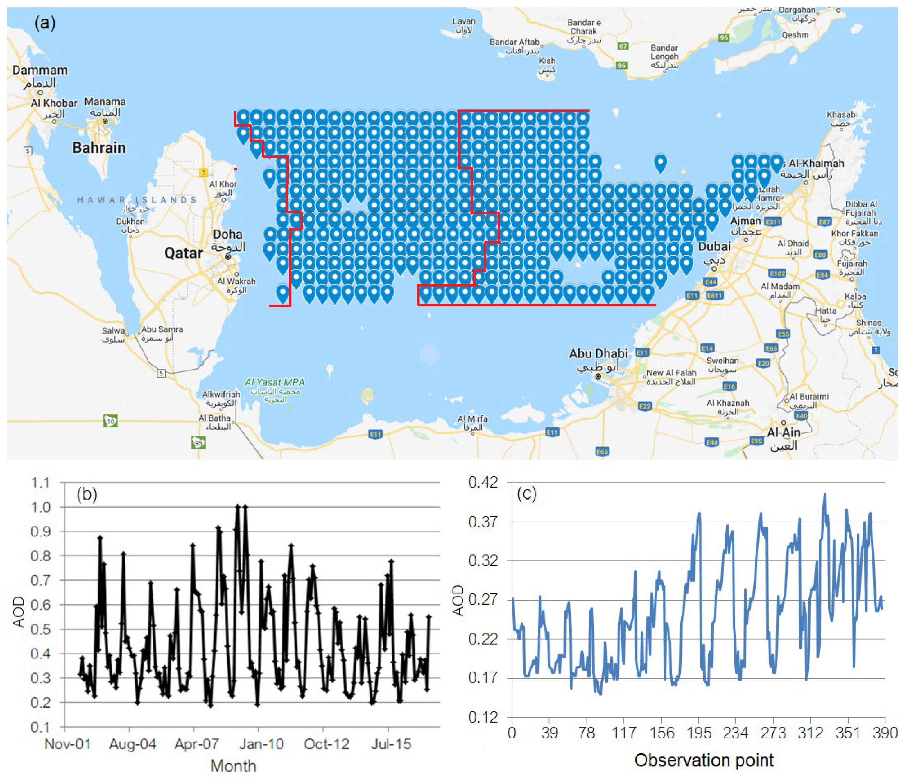
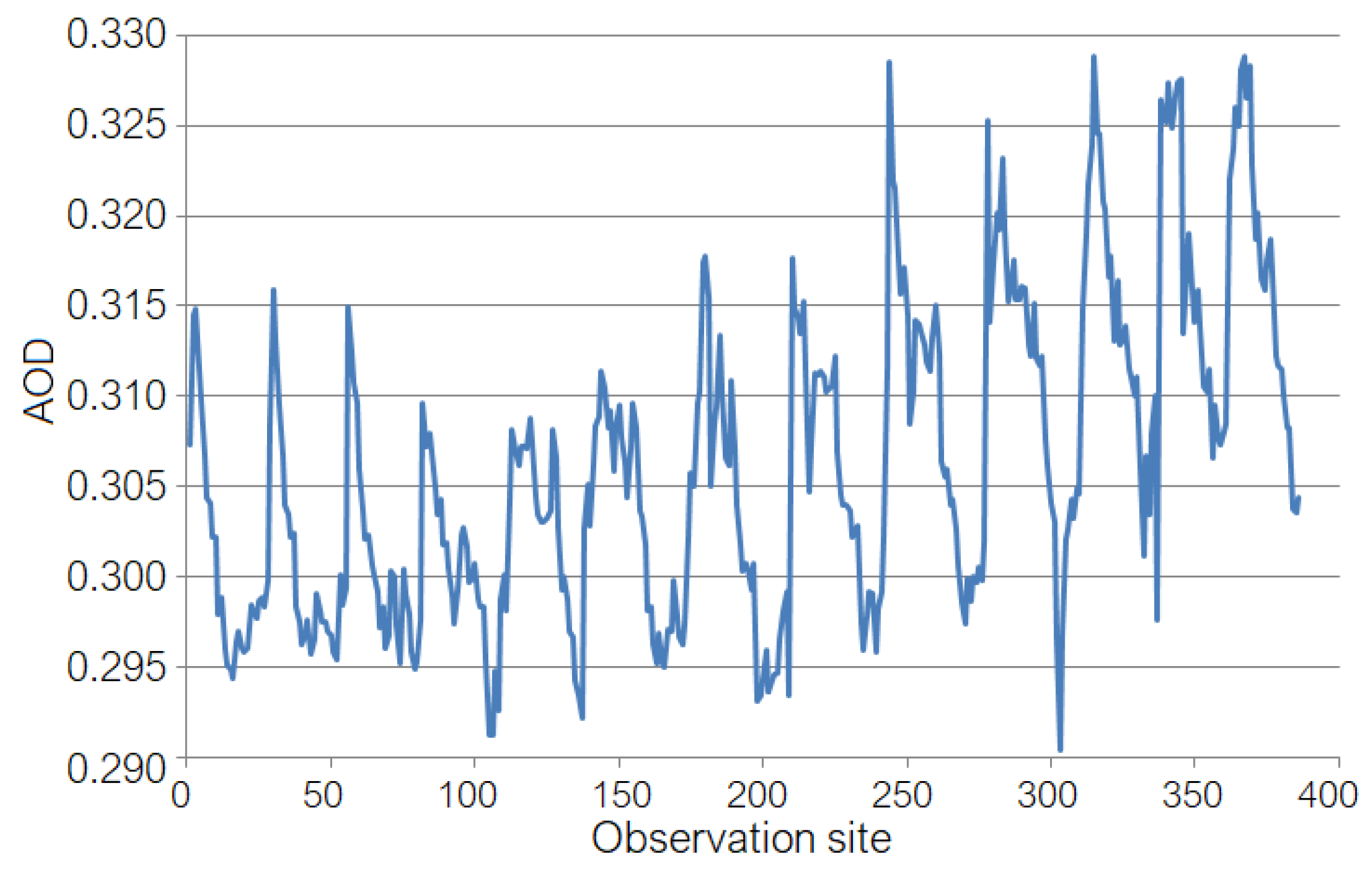
Data used in this study are monthly AOD series retrieved by Terra MODIS (at a wavelength of 412 nm) at 387 points from July 2002 to April 2017 in the Arabian Gulf Region (Figure 1a), between 24.95–26.25 latitudes and 51.55–55.75 longitudes. The series retrieved at the point of coordinates 26.15 latitude and 51.55 longitude is presented in Figure 1b and the series recorded in January 2003 is shown in Figure 1c.
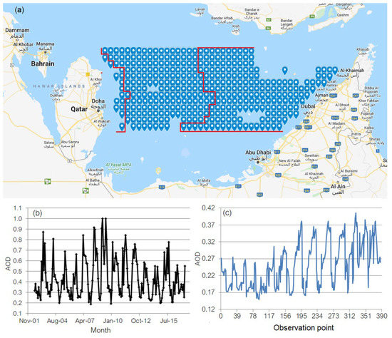
Figure 1.
(a) Observation area (https://www.google.com/mymaps/, 2022); (b) the series retrieved at the point of coordinates 26.15 latitude and 51.55 longitude (SITS); (c) series recorded in January 2003 (TITS).
The sites are ordered in increasing order in latitude, and subsequently, by decrease latitude, from the left corner on the map of the studied region to the lower right corner. Details on the study area may be found in [4,40,41]. The coordinates of the sampling points are given in Table S1 in the Supplementary Materials. Data have been organized in a matrix, X, whose columns contain the AOD at each point, and the lines contain the monthly values at the observation points.
3. Results and Discussion
3.1. PCA and Clustering
Table 1 shows the computed eigenvalues greater than 1, the proportion of the variance explained by each component, and the cumulative proportion of the variance explained for SITS.

Table 1.
Eigen-analysis of the correlation matrix of SITS.
Although eight eigenvalues are greater than 1, the first component (PC1) explains 90.20% of the variance within this set. The second component (PC2) explains only 2.8% of the variance within SITS, while the others have even smaller contributions. The first two principal components (PCs) are enough to extract the essential information within the time series set, which proves to be highly PCA compressible. Only 9.80% of the variance within this data is outside the direction of the first dominant PC, and 6.90% is outside the plane determined by PC1 and PC2. These small percentages reveal that the series similarity (linear dependence) is high in this set because the data points agglomerate along with PC1. Therefore, the sand aerosols over the Arabian Gulf have a regional nature, the AOD values being relatively similar (linearly dependent) across the analyzed area.
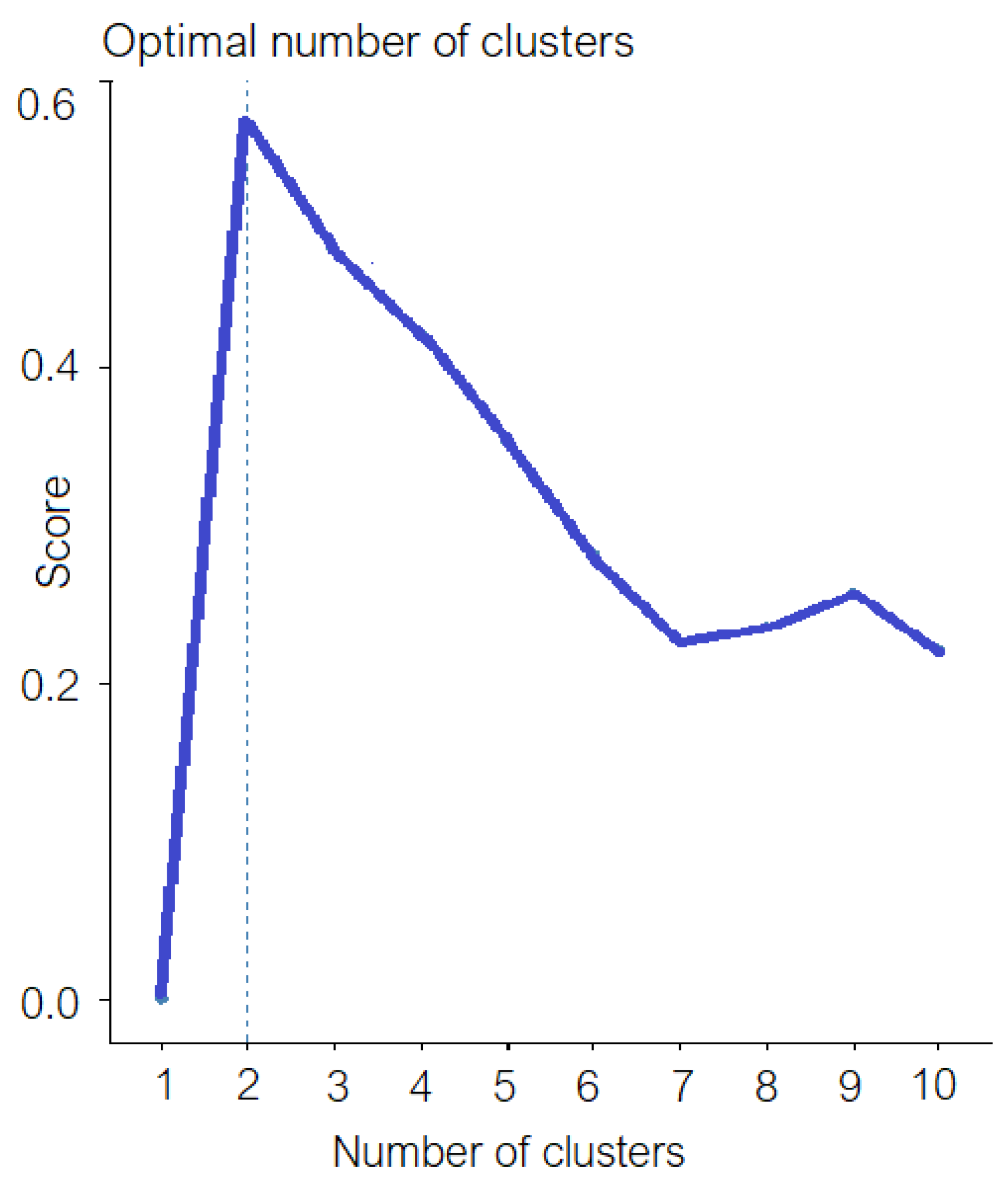
The optimal number of clusters—two—was selected after running the NbClust package in R. Figure 2 displays the silhouette chart (one of the 30 methods run). The agglomerative clustering has been performed for SITS setting the number of clusters equal to two. The computed agglomerative coefficient was 0.7678, indicating a good partition of the series in two sets. The highest this coefficient is, the better the clustering is.
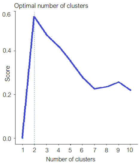
Figure 2.
The silhouette chart. The dotted line indicates the optimum number of clusters (two).
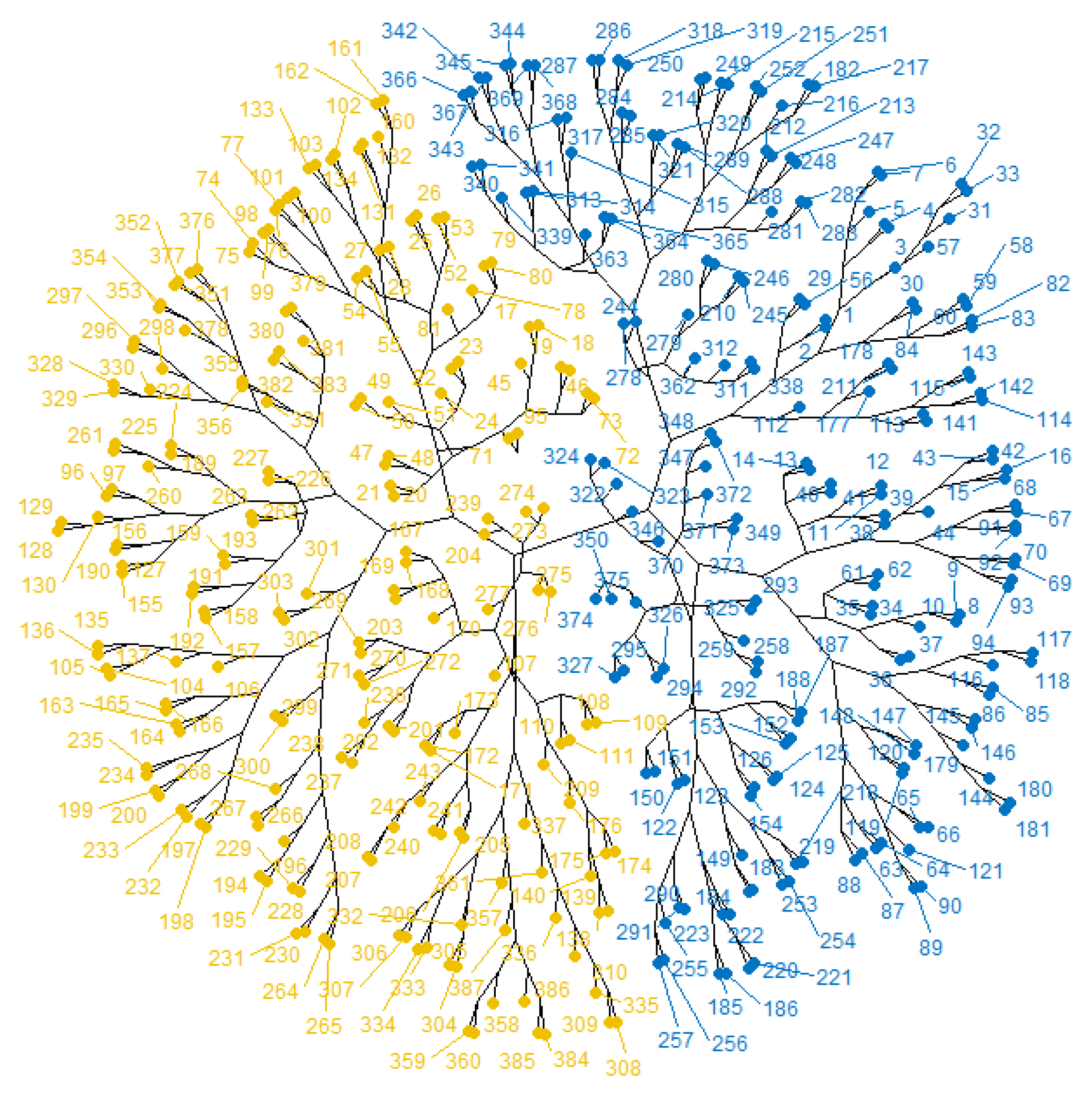
The dendrogram displaying the groups of the observation points is presented in Figure 3.
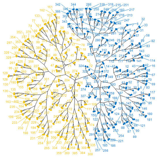
Figure 3.
The dendrogram for classification of SITS. The elements in different clusters are in different colors.
Analyzing the elements in the clusters related to the positions of the points on the map (Figure 1a and Supplementary Table S1), results in that one cluster contains the points situated on the eastern side of the region and (very few) near the Qatar shore, while the second one contains the rest of the locations. So, one cluster contains the sites situated in the direction where the Shamal blows—between the red borders in Figure 1.
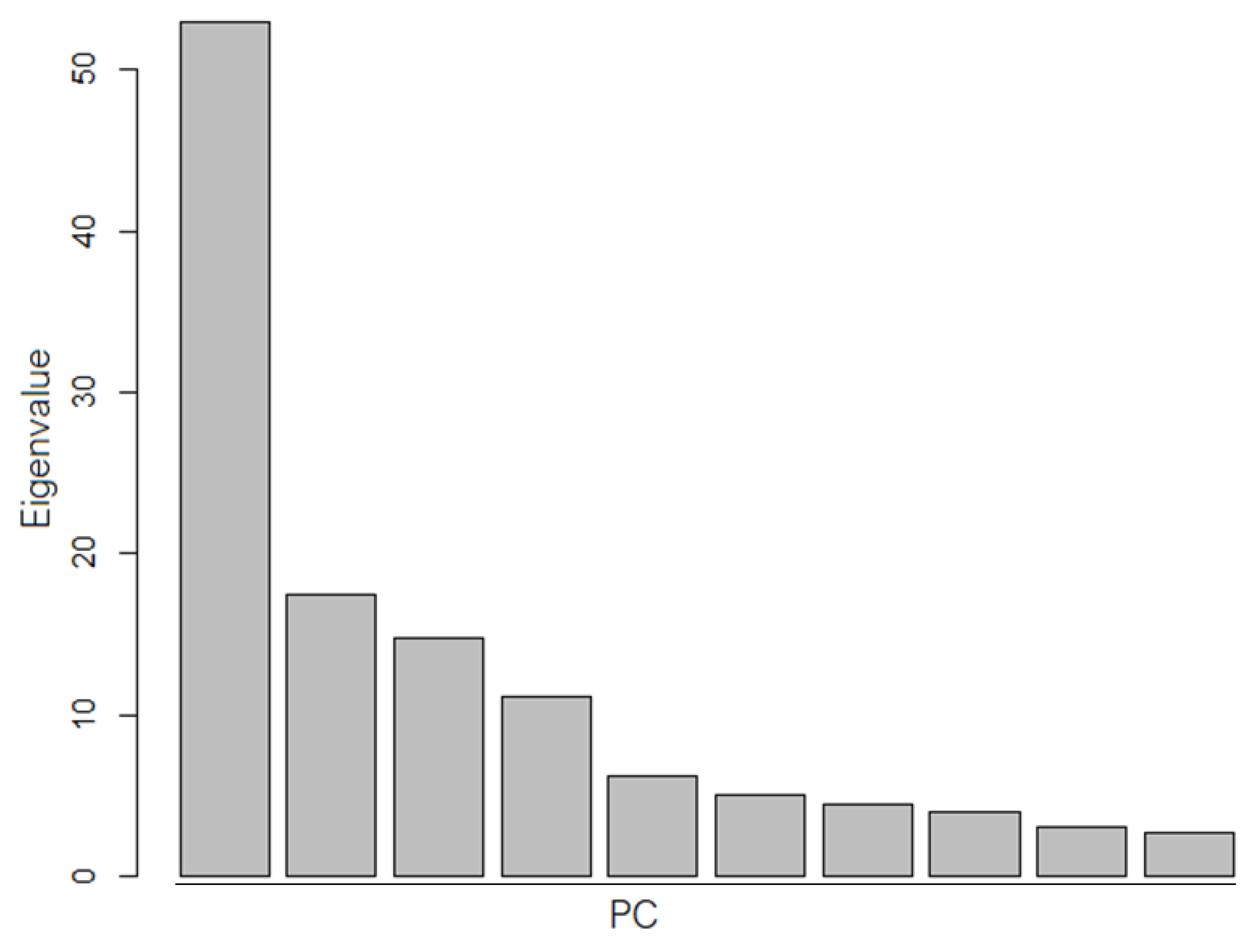
Figure 4 shows the scree plot of the TITS (the lines of the data matrix). The computation found 25 eigenvalues greater than one, with only six PCs explaining 60.5% of the variance.
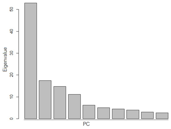
Figure 4.
The scree plot for TITS.
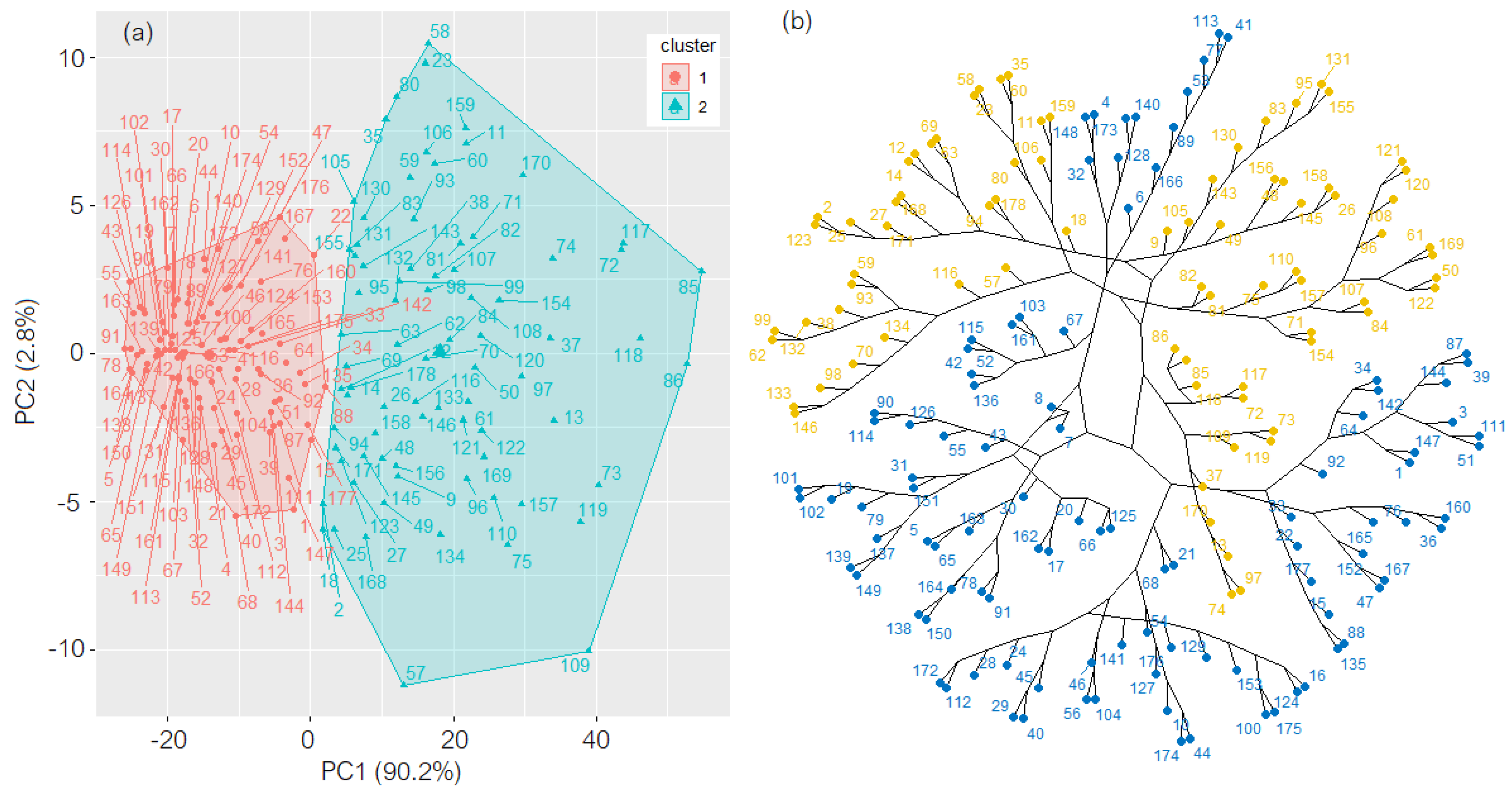
The majority principle decided that the number of clusters to classify the series is also two for the TITS. Figure 5 contains the elements in the clusters and the dendrograms for the TITS. The agglomerative clustering provided an agglomerative coefficient of 0.92802, which indicates a strong separation between the groups.
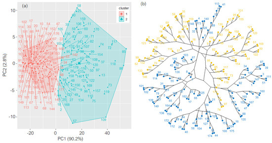
Figure 5.
(a) Clusters (the values on the axes represent the scores on PC2 and PC1) and (b) the dendrogram from the hierarchical clustering of TITS. The elements in different clusters are in different colors.
Comparing the clusters’ content, it resulted that one of them mainly contains the series recorded in the summer months (March to August), while the other contains the rest. So, the classification is related to seasonality.
3.2. Estimating the RTS and TTS
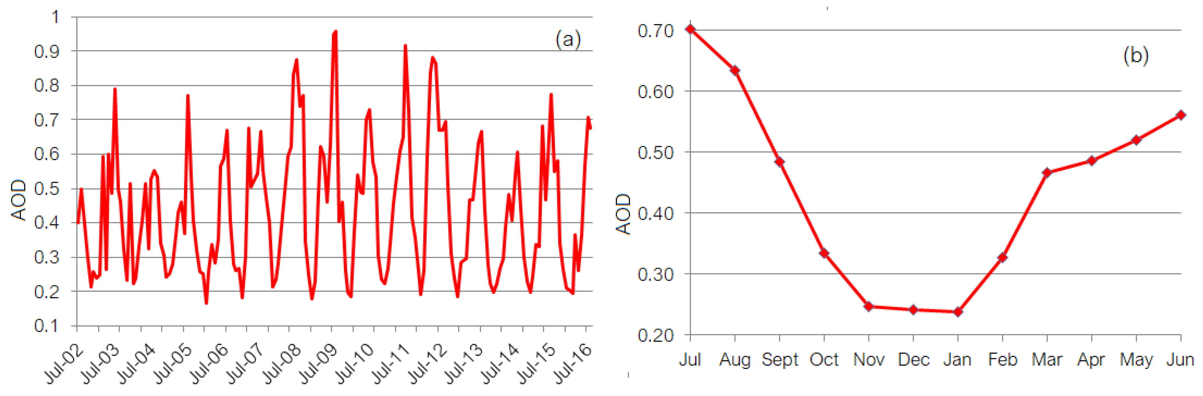
Taking into account the results from the previous section, the RTS has been computed by applying the algorithm (I)–(V) described in Section 2 to SITS (columns in the matrix X). The AOD’s RTS (as a function of time) is presented in Figure 6a. One can remark on the periodic behavior of this series, whose highest values of the AOD’s RTS are primarily recorded in July, while the lowest is in November–January.
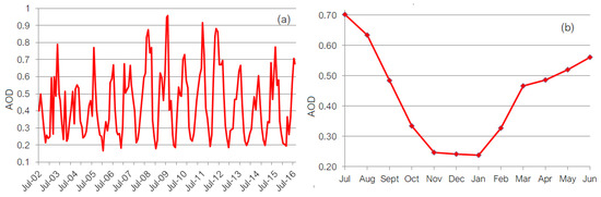
Figure 6.
(a). The AOD ‘s RTS; (b) AOD’s RTS monthly average.
Figure 6b shows that the AOD’s RTS monthly average value for July is about three times higher than the corresponding average values for November–January. This result is in concordance with those of Abuelgasim and Farahat [26] and Yoon et al. [56], which indicated a significant increase of AOD over the Gulf Region, especially in summer, related to the dust abundance [39,40,41,57,58].
The trend and level stationarity hypotheses could not be rejected for the RTS (p-value > 0.1, in both cases) when applying the KPSS test. This means that the RTS does not present a variation in trend or level.
The TTS (Figure 7) was built from the TITS (the transposed matrix, YT) and the same algorithm.

Figure 7.
The TTS of AOD obtained running the algorithm from Section 3 for TITS.
The aspect of TTS, with peaks and troughs is related not only by the monthly characteristics of the AOD (higher dust quantities in summer, and lower in winter), but also to the position of the sampling points (Figure 1a) in the direction NW-SE in which Shamal blows.
The non-stationarity in the level and trend stationarity are emphasized by the results of the KPSS test, whose p-values are lower than 0.01 (for level-stationarity) and 0.12376 (for trend-stationarity).
The goodness-of-fit indicators are tools for assessing the fit quality. The lower their values are, the better the fit is. For a correct model quality assessment, using more than one indicator is recommended. For example, MSE can be influenced by values that significantly deviate from the average. Therefore, three goodness-of-fit indicators have been utilized here—MAE, MSE, and MAPE—the last one being non-dimensional, so it is more reliable for comparisons between the two models.
All the values of the goodness-of-fit indicators corresponding to the RTS and TTS are all very low (Table 2). They indicate a better fit for RTS than for TTS when reported to the average indicators. Indeed, the mean values of MAE (MSE and MAPE, respectively) are 0.1724/0.0326 = 5.29 (21.88 and 4.38 times higher, respectively) for TTS than for RTS. The minimum MAE and MSE are also lower for RTS compared to TTS, but the min MAPE is higher for RTS.
Table 2.
Goodness of fit indicators of RTS and TTS.
The maximum values of MAE (max MSE and max MAPE, respectively) is 11.15 (55.32 and 4.84, respectively) times higher for RTS than for TTS, indicating a higher variability at the temporal scale than at the spatial one.
This means that RTS better represents the individual series than TTS, so there is a higher homogeneity of the SITS than the TITS. The result is in concordance with the findings related to the seasonal variability of AOD [26].
4. Conclusions
This study extended our previous research on the aerosol radius, using the AOD series collected during the same period at the same sampling points in the Gulf Region. The novelty of the research consists of a dual analysis in time and space and the detection of RTS and TTS that characterizes the AOD behavior over the study zone.
The approach combined the PCA with a new algorithm, building the RTS and TTS series based on the classification provided by the clustering.
It was found that a single principal component explains more than 90% of the variance of SITS, indicating that the series are agglomerated along with PC1. The TITS are scattered (the first six dominant principal components accounting for only 60.5% of the variance in the sets). Still, both RTS and TTS fit data well and are trend stationary.
We intend to extend the research to sets of series with missing data, given that most of the available records present gaps.
Supplementary Materials
The following supporting information can be downloaded at: https://www.mdpi.com/article/10.3390/atmos13060857/s1, Table S1: Data series and the coordinates of the locations.
Funding
This research received funding from the research fund of Transilvania University of Brașov, Romania.
Institutional Review Board Statement
Not applicable.
Informed Consent Statement
Not applicable.
Data Availability Statement
Data can be freely downloaded from the site https://modis.gsfc.nasa.gov/data/ (accessed on 10 July 2017).
Conflicts of Interest
The authors declare no conflict of interest.
References
- Yassin, M.F.; Almutairi, S.K.; Al-Hemoud, A. Dust storms backward trajectories and source identification over Kuwait. Atmos. Res. 2018, 212, 158–171. [Google Scholar] [CrossRef]
- Grini, A.; Zender, C.S.; Colarco, P. Saltation sandblasting behavior during mineral dust aerosol production. Geophys. Res. Lett. 2002, 29, 15-1–15-4. [Google Scholar] [CrossRef] [Green Version]
- Shao, Y.; Raupach, M.R.; Findlater, P.A. Effect of saltation bombardment on the entrainment of dust by wind. J. Geophys. Res. 1993, 98, 12719–12726. [Google Scholar] [CrossRef] [Green Version]
- Bărbulescu, A.; Nazzal, Y.; Howari, F. Statistical analysis and estimation of the regional trend of aerosol size over the Arabian Gulf Region during 2002–2016. Sci. Rep. 2018, 8, 9571. [Google Scholar] [CrossRef] [PubMed] [Green Version]
- Astitha, M.; Lelieveld, J.; Abdel Kader, M.; Pozzer, A.; de Meij, A. Parameterization of dust emissions in the global atmospheric chemistry-climate model EMAC: Impact of nudging and soil properties. Atmos. Chem. Phys. 2012, 12, 11057–11083. [Google Scholar] [CrossRef] [Green Version]
- Ganor, E.; Osetinsky, I.; Stupp, A.; Alpert, P. Increasing trend of African dust, over 49 years, in the eastern Mediterranean. J. Geophys. Res. 2010, 115, D07201. [Google Scholar] [CrossRef] [Green Version]
- Smoydzin, L.; Fnais, M.; Lelieveld, J. Ozone pollution over the Arabian Gulf—Role of meteorological conditions. Atmos. Chem. Phys. Discuss. 2012, 12, 6331–6361. [Google Scholar] [CrossRef] [Green Version]
- Haywood, J.; Francis, P.; Osborne, S.; Glew, M.; Loeb, N.; Highwood, E.; Tanré, D.; Myhre, G.; Formenti, P.; Hirst, E. Radiative properties and direct radiative effect of Saharan dust measured by the C-130 aircraft during SHADE: 1. Solar spectrum. J. Geophys. Res. 2003, 108, 8577. [Google Scholar] [CrossRef] [Green Version]
- Mahowald, N.; Albani, S.; Kok, J.K.; Engelstaeder, M.; Scanza, R.; Ward, D.S.; Flanner, M.G. The size distribution of desert dust aerosols and its impact on the Earth system. Aeolian Res. 2014, 15, 53–71. [Google Scholar] [CrossRef] [Green Version]
- Ginoux, P.; Prospero, J.M.; Gill, E.T.; Hsu, N.C.; Zhai, M. Global-scale attribution of anthropogenic and natural dust sources and their emission rates based on MODIS Deep Blue aerosol products. Rev. Geophys. 2012, 50(3), RG3005. [Google Scholar] [CrossRef]
- Chen, S.; Huang, J.; Li, J.; Jia, R.; Kang, L.; Ma, X.; Xie, T. Comparison of dust emission, transport, and deposition between the Taklimakan desert and Gobi desert from 2007 to 2011. Sci. China Earth Sci. 2017, 60, 1338–1355. [Google Scholar] [CrossRef]
- Doyle, M.; Dorling, S. Visibility trends in the UK 1950–1997. Atmos. Environ. 2002, 36, 3161–3172. [Google Scholar] [CrossRef]
- Deng, X.; Tie, X.; Wu, D.; Zhou, X.; Bi, X.; Tan, H.; Li, F.; Jiang, C. Long-term trend of visibility and its characterizations in the Pearl River Delta (PRD) region, China. Atmos. Environ. 2008, 42, 1424–1435. [Google Scholar] [CrossRef]
- Goudie, A.S.; Middleton, N.J. Desert Dust in the Global System; Springer: Berlin, Germany, 2006. [Google Scholar]
- Middleton, N.J. A geography of dust storms in Southwest Asia. J. Climatol. 1986, 6, 183–196. [Google Scholar] [CrossRef]
- Notaro, M.; Alkolibi, F.; Fadda, E.; Bakhrjy, F. Trajectory analysis of Saudi Arabia dust storm. J. Geophys. Res. Atmos. 2013, 118, 6028–6043. [Google Scholar] [CrossRef]
- Shao, Y. A model for mineral dust emission. J. Geophys. Res. Atmos. 2001, 106, 20239–20254. [Google Scholar] [CrossRef]
- Yu, Y.; Notaro, M.; Liu, Z.; Wang, F.; Alkolibi, F.; Fadda, E.; Bakhrjy, F. Climatic controls on the interannual to decadal variability in Saudi Arabian dust activity: Toward the development of a seasonal dust prediction model. J. Geophys. Res. Atmos. 2015, 120, 1739–1758. [Google Scholar] [CrossRef]
- Arfan Ali, M.; Nichol, J.E.; Bilal, M.; Qiu, Z.; Mazhar, U.; Wahiduzzaman, M.; Almazroui, M.; Nazrul Islam, M. Classification of aerosols over Saudi Arabia from 2004–2016. Atmos. Environ. 2020, 241, 117785. [Google Scholar] [CrossRef]
- Mohammadpour, K.; Rashki, A.; Sciortino, M.; Kaskaoutis, D.G.; Boloorani, A.D. A statistical approach for identification of dust-AOD hotspots climatology and clustering of dust regimes over Southwest Asia and the Arabian Sea. Atmos. Pollut. Res. 2022, 13, 01395. [Google Scholar] [CrossRef]
- Mohammadpour, K.; Sciortino, M.; Kaskaoutis, D.G. Classification of weather clusters over the Middle East associated with high atmospheric dust-AODs in West Iran. Atmos. Res. 2021, 259, 105682. [Google Scholar] [CrossRef]
- Sogacheva, L.; Rodriguez, E.; Kolmonen, P.; Virtanen, T.H.; Saponaro, G.; de Leeuw, G.; Georgoulias, A.K.; Alexandri, G.; Kourtidis, K.; van der A, R.J. Spatial and seasonal variations of aerosols over China from two decades of multi-satellite observations. Part II: AOD time series for 1995–2017 combined from ATSR, ADV and MODIS C6.1 for AOD tendencies estimation. Atmos. Chem. Phys. 2018, 18, 16631–16652. [Google Scholar] [CrossRef] [Green Version]
- Li, J.; Carlson, B.E.; Lacis, A.A. Application of spectral analysis techniques in the intercomparison of aerosol data: 1. An EOF approach to analyze the spatial-temporal variability of aerosol optical depth using multiple remote sensing data sets. J. Geophys. Res. Atmos. 2013, 118, 8640–8648. [Google Scholar] [CrossRef]
- Li, J.; Carlson, B.E.; Lacis, A.A. Application of spectral analysis techniques in the intercomparison of aerosol data: Part III. Using combined PCA to compare spatiotemporal variability of MODIS, MISR, and OMI aerosol optical depth. J. Geophys. Res. Atmos. 2014, 119, 4017–4042. [Google Scholar] [CrossRef] [Green Version]
- Ma, Q.; Zhang, Q.; Wang, Q.; Yuan, X.; Yuan, R.; Luo, C. A comparative study of EOF and NMF analysis on downward trend of AOD over China from 2011 to 2019. Environ. Pollut. 2021, 288, 117713. [Google Scholar] [CrossRef] [PubMed]
- Abuelgasim, A.; Farahat, A. Effect of dust loadings, meteorological conditions, and local emissions on aerosol mixing and loading variability over highly urbanized semiarid countries: United Arab Emirates case study. J. Atmos. Sol. Terr. Phys. 2019, 199, 105215. [Google Scholar] [CrossRef]
- Kim, J.; Lee, J.; Lee, H.C.; Higurashi, A.; Takemura, T.; Song, C.H. Consistency of the aerosol type classification from satellite remote sensing during the Atmospheric Brown Cloud—East Asia Regional Experiment campaign. J. Geophys. Res. 2007, 112, D22S33. [Google Scholar] [CrossRef]
- Hsu, N.C.; Gautam, R.; Sayer, A.M.; Bettenhausen, C.; Li, C.; Jeong, M.J.; Tsay, S.-C.; Holben, B.N. Global and regional trends of aerosol optical depth over land and ocean using SeaWiFS measurements from 1997 to 2010. Atmos. Chem. Phys. 2012, 12, 8037–8053. [Google Scholar] [CrossRef] [Green Version]
- De Meij, A.; Pozzer, A.; Lelieveld, J. Trend analysis in aerosol optical depths and pollutant emission estimates between 2000 and 2009. Atmos. Environ. 2012, 51, 75–85. [Google Scholar] [CrossRef]
- Dubovik, O.; Holben, B.; Eck, T.F.; Smirnov, A.; Kaufman, Y.J.; King, M.D.; Tanré, D.; Slutsker, I. Variability of Absorption and Optical Properties of Key Aerosol Types Observed in Worldwide Locations. J. Atmos. Sci. 2002, 59, 590–608. [Google Scholar] [CrossRef]
- Ridley, D.A.; Heald, C.L.; Kok, J.F.; Zhao, C. An observationally constrained estimate of global dust aerosol optical depth. Atmos. Chem. Phys. 2016, 16, 15097–15117. [Google Scholar] [CrossRef] [Green Version]
- Smirnov, A.; Holben, B.; Dubovik, O.; O’Neill, N.T.; Eck, T.F.; Westphal, D.L.; Goroch, A.K.; Pietras, C.; Slutsker, I. Atmospheric Aerosol Optical Properties in the Persian Gulf Region. J. Atmos. Sci. 2002, 59, 620–634. [Google Scholar] [CrossRef]
- Krishna Moorthy, K.; Babu, S.S.; Satheesh, S.K.; Lal, S.; Sarin, M.M.; Ramachandran, S. Climate implications of atmospheric aerosols and trace gases: Indian Scenario. In Climate Sense; Asrar, G., Ed.; Tudor Rose: Leicester, UK, 2009. [Google Scholar]
- Al-Taani, A.A.; Nazzal, Y.; Howari, F.; Iqbal, J.; Bou-Orm, N.; Xavier, C.M.; Bărbulescu, A.; Sharma, M.; Dumitriu, C.S. Contamination assessment of heavy metals in agricultural soil, in the Liwa area (UAE). Toxics 2021, 9, 53. [Google Scholar] [CrossRef] [PubMed]
- Bărbulescu, A.; Dumitriu, C.Ș. Assessing the water quality by statistical methods. Water 2021, 13, 1026. [Google Scholar] [CrossRef]
- Bărbulescu, A.; Barbeș, L.; Dumitriu, C.S. Assessing the water pollution of Brahmaputra River using water quality indexes. Toxics 2021, 9, 297. [Google Scholar] [CrossRef] [PubMed]
- Bărbulescu, A.; Dumitriu, C.S.; Ilie, I.; Barbes, S.B. Influence of Anomalies on the Models for Nitrogen Oxides. Atmosphere 2022, 13, 558. [Google Scholar] [CrossRef]
- Nazzal, Y.H.; Bărbulescu, A.; Howari, F.; Al-Taani, A.A.; Iqbal, J.; Xavier, C.M.; Sharma, M.; Dumitriu, C.S. Assessment of metals concentrations in soils of Abu Dhabi Emirate using pollution indices and multivariate statistics. Toxics 2021, 9, 95. [Google Scholar] [CrossRef] [PubMed]
- Aldababseh, A.; Temimi, M. Analysis of the long-term variability of poor visibility events in the UAE and the link with the climate dynamics. Atmosphere 2017, 8, 242. [Google Scholar] [CrossRef] [Green Version]
- Nazzal, Y.; Bărbulescu, A.; Howari, F.M.; Yousef, A.; Al-Taani, A.A.; Al Aydaroos, F.; Naseem, M. New insight to dust storm from historical records, UAE. Arab. J. Geosci. 2019, 12, 396. [Google Scholar] [CrossRef]
- Bărbulescu, A.; Nazzal, Y. Statistical analysis of the dust storms in the United Arab Emirates. Atmos. Res. 2020, 231, 104669. [Google Scholar] [CrossRef]
- Lorenz, E.N. Empirical Orthogonal Functions and Statistical Weather Prediction; Science Report No. 1; MIT: Cambridge, MA, USA, 1956; 49p. [Google Scholar]
- Fiore, A.M.; Jacob, D.J.; Mathur, R.; Martin, R.V. Application of empirical orthogonal functions to evaluate ozone simulations with regional and global models. J. Geophys. Res. Atmos. 2009, 108, 4431. [Google Scholar] [CrossRef]
- Martin, R.V.; Jacob, D.J.; Logan, J.A.; Ziemke, J.M.; Washington, R. Detection of a lightning influence on tropical tropospheric ozone. Geophys. Res. Lett. 2000, 27, 1639–1842. [Google Scholar] [CrossRef]
- Abdi, H.; Williams, L. Principal Component Analysis. Wires Comput. Stat. 2010, 2, 433–458. [Google Scholar] [CrossRef]
- Zou, H.; Hastie, T.; Tibshirani, R. Sparse principal component analysis. J. Comput. Graph. Stat. 2006, 15, 265–286. [Google Scholar] [CrossRef] [Green Version]
- Abid, A.; Zhang, M.J.; Bagaria, V.K.; Zou, J. Exploring patterns enriched in a dataset with contrastive principal component analysis. Nat. Commun. 2018, 9, 2134. [Google Scholar] [CrossRef] [PubMed] [Green Version]
- Trendafilov, N.T. Stepwise estimation of common principal components. Comput. Stat. Data Anal. 2010, 54, 3446–3457. [Google Scholar] [CrossRef]
- Kutzbach, J. Empirical eigenvectors in sea-level pressure, surface temperature, and precipitation complexes over North America. J. Appl. Meteorol. 1967, 6, 791–802. [Google Scholar] [CrossRef]
- Cattell, R.B. The Scree test for the number of factors. Multivar. Behav. Res. 1966, 1, 245–276. [Google Scholar] [CrossRef]
- Kaiser, H.F. The Application of Electronic Computers to Factor Analysis. Educ. Psychol. Meas. 1960, 20, 141–151. [Google Scholar] [CrossRef]
- Jolliffe, I. Principal Component Analysis, 2nd ed.; Springer: Berlin/Heidelberg, Germany, 2002. [Google Scholar]
- Rousseeuw, P.J. Silhouettes: A graphical aid to the interpretation and validation of cluster analysis. Comput. Appl. Math. 1987, 20, 53–65. [Google Scholar] [CrossRef] [Green Version]
- Charrad, M.; Ghazzali, N.; Boiteau, V.; Niknafs, A. Package ‘NbClust’. Available online: https://cran.r-project.org/web/packages/NbClust/NbClust.pdf (accessed on 25 September 2020).
- Kwiatkowski, D.; Phillips, P.C.B.; Schmidt, P.; Shin, Y. Testing the null hypothesis of stationarity against the alternative of a unit root. J. Econometr. 1992, 54, 159–178. [Google Scholar] [CrossRef]
- Yoon, J.; von Hoyningen-Huene, W.; Kokhanovsky, A.A.; Vountas, M.; Burrows, J.P. Trend analysis of aerosol optical thickness and Ångström exponent derived from the global AERONET spectral observations. Atmos. Meas. Tech. 2012, 5, 1271–1299. [Google Scholar] [CrossRef] [Green Version]
- Karagulian, F.; Temimi, M.; Ghebreyesus, D.; Weston, M.; Kondapalli, N.K.; Valappil, V.K.; Aldababesh, A.; Lyapustin, A.; Chaouch, N.; Al Hammadi, F.; et al. Analysis of a severe dust storm and its impact on air quality conditions using WRF-Chem modeling, satellite imagery, and ground observations. Air Qual. Atmos. Health 2019, 12, 453–470. [Google Scholar] [CrossRef] [Green Version]
- Nazzal, Y.; Orm, N.B.; Bărbulescu, A.; Howari, F.; Sharma, M.; Badawi, A.E.; Al-Taani, A.A.; Iqbal, J.; El Ktaibi, F.; Xavier, C.M.; et al. Study of atmospheric pollution and health risk assessment. A case study for the Sharjah and Ajman Emirates (UAE). Atmosphere 2021, 12, 1442. [Google Scholar] [CrossRef]
Publisher’s Note: MDPI stays neutral with regard to jurisdictional claims in published maps and institutional affiliations. |
© 2022 by the author. Licensee MDPI, Basel, Switzerland. This article is an open access article distributed under the terms and conditions of the Creative Commons Attribution (CC BY) license (https://creativecommons.org/licenses/by/4.0/).