Article

Influence of Anomalies on the Models for Nitrogen Oxides and Ozone Series

by
Alina Bărbulescu
1,
Cristian Stefan Dumitriu
2,*,
Iulia Ilie
3 and
Sebastian-Barbu Barbeş
4
1
Department of Civil Engineering, Transilvania University of Brașov, 5 Turnului Str., 900152 Brașov, Romania
2
SC Utilnavorep SA, 55, Aurel Vlaicu Av., 900055 Constanta, Romania
3
Siemens Romania, 13A, Bd. Garii, 900055 Brașov, Romania
4
Doctoral School of Civil Engineering, Technical University of Civil Engineering, 122-124 Lacul Tei Bvd., 020396 Bucharest, Romania
*
Author to whom correspondence should be addressed.
Atmosphere 2022, 13(4), 558; https://doi.org/10.3390/atmos13040558
Submission received: 2 March 2022 / Revised: 22 March 2022 / Accepted: 28 March 2022 / Published: 30 March 2022
(This article belongs to the Special Issue Assessing Atmospheric Pollution and Its Impacts on the Human Health)

Abstract

:
Nowadays, observing, recording, and modeling the dynamics of atmospheric pollutants represent actual study areas given the effects of pollution on the population and ecosystems. The existence of aberrant values may influence reports on air quality when they are based on average values over a period. This may also influence the quality of models, which are further used in forecasting. Therefore, correct data collection and analysis is necessary before modeling. This study aimed to detect aberrant values in a nitrogen oxide concentration series recorded in the interval 1 January–8 June 2016 in Timisoara, Romania, and retrieved from the official reports of the National Network for Monitoring the Air Quality, Romania. Four methods were utilized, including the interquartile range (IQR), isolation forest, local outlier factor (LOF) methods, and the generalized extreme studentized deviate (GESD) test. Autoregressive integrated moving average (ARIMA), Generalized Regression Neural Networks (GRNN), and hybrid ARIMA-GRNN models were built for the series before and after the removal of aberrant values. The results show that the first approach provided a good model (from a statistical viewpoint) for the series after the anomalies removal. The best model was obtained by the hybrid ARIMA-GRNN. For example, for the raw NO2 series, the ARIMA model was not statistically validated, whereas, for the series without outliers, the ARIMA(1,1,1) was validated. The GRNN model for the raw series was able to learn the data well: R2 = 76.135%, the correlation between the actual and predicted values (rap) was 0.8778, the mean standard errors (MSE) = 0.177, the mean absolute error MAE = 0.2839, and the mean absolute percentage error MAPE = 9.9786. Still, on the test set, the results were worse: MSE = 1.5101, MAE = 0.8175, rap = 0.4482. For the series without outliers, the model was able to learn the data in the training set better than for the raw series (R2 = 0.996), whereas, on the test set, the results were not very good (R2 = 0.473). The performances of the hybrid ARIMA–GRNN on the initial series were not satisfactory on the test (the pattern of the computed values was almost linear) but were very good on the series without outliers (the correlation between the predicted values on the test set was very close to 1). The same was true for the models built for O3.

1. Introduction

Nowadays, ambient air pollution levels and trends have become a topic of interest worldwide because primary atmospheric pollutants (APPs) constitute a risk factor for the population and ecosystems [1,2,3,4]. Therefore, monitoring air quality, especially in urban or crowded areas, is essential for controlling pollution [5] and protecting human health.
Pollutants’ dispersion into the atmosphere is a hazardous phenomenon, which is difficult to assess and sometimes unpredictable. Their diffusion depends on meteorological factors, such as the relative speed and wind direction, ambient temperature, atmospheric turbulence, and buoyant force [6,7]. The distinct mechanisms responsible for pollutant dispersion are molecular diffusion, turbulent diffusion, and transport due to wind. Generally, wind speed influences pollutants’ distribution. High concentrations of pollutants reach the atmospheric layer and remain there if the wind speed is low and uniform. Atmospheric calm creates favorable conditions for the accumulation of pollutants in the source’s vicinity [8].
Nitrogen oxides (NOx) are gases containing various amounts of nitrogen and oxygen with high reactivity. NOx represents a family of seven chemical compounds (N2O, NO, N2O2, N2O3, NO2, N2O4, N2O5) [9] Nitrogen monoxide and dioxide (NO and NO2) are the main NOx found in the atmosphere, resulting from combustion processes (from electricity generation, industrial activities, and engine exhaust). They contribute to the apparition of acid rains and favor the accumulation of nitrates in the soil, leading to ecological disequilibrium [10]. Nitrogen oxides contribute to the greenhouse effect and smog formation, reducing the visibility in urban areas and the deterioration of water quality.
Nitrogen oxide (NO) is a colorless gas and a free radical. It is important that it is monitored s it is a precursor of tropospheric ozone, nitric acid, and particulate nitrate. Although NO does not directly affect acid deposition or the climate, nitric acid and ozone and particulate nitrate do. Natural NO reduces ozone in the upper stratosphere. NO emissions from jets that fly in the stratosphere also reduce stratospheric ozone. In urban zones, NO mixing ratios reach 0.1 ppmv in the early morning but may decrease to zero by midmorning due to the reaction with ozone. Outdoor levels of NO are not regulated in any country [11].
Nitrogen dioxide (NO2) is a brown gas with a strong odor. NO2 is an intermediary between NO emission and ozone (O3) formation. It is also a precursor to nitric acid, a component of acid deposition. Natural NO2, such as natural NO, reduces O3 in the upper stratosphere. The primary source of NO2 is NO oxidation. Minor sources are fossil fuel combustion and biomass burning. During combustion or burning, NO2 emissions are about 5% to 15% of those of NO. In urban regions, NO2 mixing ratios range from 0.1 to 0.25 ppmv. Outdoors, NO2 is more relevant during the early morning than during midday or afternoon because sunlight breaks down most NO2 past midmorning, which is usually the opposite to ozone [12].
NO’s toxicity is four times lower than that of NO2. Children are the most affected by exposure to nitrogen dioxide. NO2 is very toxic for the population and animals [10,13]. Exposure to low concentrations of NO2 affects lung tissue, and high pollutant concentrations may be fatal. The population exposed to low concentrations of nitrogen oxides may experience respiratory issues for a long time [2,4].
Therefore, outdoor levels of NO2 are now regulated in many countries, including Romania [12,14,15]. Ozone is a relatively colorless gas at typical mixing ratios. O3 exhibits an odor when its mixing ratio exceeds 0.02 ppmv. In urban smog, it is considered an air pollutant because of its harmful effects on humans, animals, plants, and materials. In the stratosphere, ozone’s absorption of UV radiation provides a protective shield for terrestrial life. O3 is not emitted. Its only source in the air is chemical reaction. O3 is a pollutant produced in the atmosphere, and therefore it is not necessarily related to urban or industrial areas and may be seen in suburban or rural areas, in downwind zones from where the precursors are emitted. In urban air, ozone mixing ratios range from less than 0.01 ppmv at night to 0.5 ppmv (during the afternoon, downwind from the most polluted cities worldwide), with typical values of 0.15 ppmv during moderately polluted afternoons. It has a typical daily cycle characteristic of the positions with respect to the topography and the location where the precursors are emitted. Peak ozone mixing ratios are around 10 ppmv in the stratosphere [11].
In the last decade, special attention has been paid to mathematical modeling, the study of the pollutants diffusion from the atmosphere, developing new control systems, and reducing environmental pollution [16,17]. The diversity of actual models has imposed extraordinary rigor on their understanding and expanded their types for correct application depending on local or regional air pollution particularities. The transport and dispersion of pollutants in the atmosphere are complex phenomena that are not easy to translate into mathematical calculation systems, so many algorithms are accepted by simplifying hypotheses [18]. Under these conditions, the results of the estimates are more or less close to reality. Each model has its limits. The volume, type of input data, and mathematical complexity largely depend on the researchers’ abilities because the data quality, accuracy, and discretization affect the integrity of the simulation results [19].
Modeling of the dissipation of NOx from different sources has been achieved using different models, such as, for example, CALPUFF [20] (dispersion of traffic emissions in urban zones). Fallah-Shorshani et al. [21] used two air quality models to simulate local atmospheric dissipation of NOx and its transformation to NO2 using the Gaussian puff (CALPUFF) and street-canyon model (SIRANE). The SIRANE model is based on transformations involving NO, NO2, and O3 (in the Leighton cycle). Shekarrizfard et al. [22] reported CALMET-CALPUFF for the assessment of the effects of a regional transit policy on air quality and population exposure. Soulhac et al. [23] utilized the SIRANE dispersion model to assess the transfer of pollutants within and out of an urban canopy.
Stochastic models are statistical or semi-empirical techniques for estimating trends, periodicity, and the interrelationship between air quality and atmospheric measurements, and forecasting air pollution episodes. These models are instrumental in real-time forecasting or relatively short periods, where available information from measurements is relevant (immediate estimates) [24]. The most well-known model is the Box–Jenkins approach (for example, ARIMA and SARIMA).
Gocheva-Ilieva et al. [17] examined the concentrations of NO, NO2, NOx, and ground-level O3 in a town in Bulgaria for one year using hourly data. The obtained SARIMA models demonstrated a very good fitting performance and short-term predictions for the next 72 h.
Kumar and Jain [25] used ARIMA, after a suitable variance stabilizing transformation of the concentration time series (O3, CO, NO, and NO2), to model data collected at a traffic station in Delhi (India). Zhu [26] compared the ARIMA and exponential smoothing models on 2014 concentrations of NO2 and O3 in the Yanqing county, Beijing, China. Munir and Mayfield [27] used auto-regressive integrated moving average with exogenous variables (ARIMAX) to model the distributions and temporal variability of NO2 concentrations in Sheffield, UK, from August 2019 to September 2020. Using cross-validation ARIMAX, the authors found a strong correlation between the predicted values and the measured concentrations (the correlation coefficient was 0.84 and RMSE was 9.90). Hajmohammadi and Heydecker [28] developed a vector autoregressive moving average model to assess the air quality in London in 2017. The authors cross-validated the model using kriging to achieve spatial interpolation of NO, NO2, and NOx, respectively. Moreover, seasonal ARMA models of the air quality across London for 30 individual stations were validated. This study established that the VARMA model is appropriate for evaluating interventions, such as the Ultra-Low Emissions Zone.
Artificial neural networks (ANNs) have been widely used for modeling processes that present high variability and nonlinearities, such as those related to air pollution. Gardner and Dorling [29] employed a multilayer perceptron (MLP) artificial network to model NO and NO2 concentrations in London and showed that the variation in emissions could be modeled using the time of day and day of the week as input variables.
Based on the literature findings, and\ given the superior performances of deterministic methods, Rahimi [30] utilized ANN to develop a model that provided accurate short-term (hourly) predictions of NOx and NO2 series in Tabriz, Iran. Dragomir et al. [31] presented an evaluation of the efficiency of artificial neural networks (ANNs) and the multiple linear regression (MLR) model for NO2 prediction in 3 scenarios (by randomly eliminating (1) 25%, (2) 50%, or (3) 75% of the observed NO2 data) in Brăila city, Romania, from 2009–2013. The analysis results demonstrated that the NO2 values estimated using MLR and ANNs were similar to the measured NO2 concentrations (the corresponding coefficients were (1) 0.580, 0.604; (2) 0.589, 0.565; and (3) 0.474, 0.483). The best outcomes were achieved for the ANN values in all scenarios.
Multilayer perceptron is a type of neural network used in the studies of Baawain and Al-Serihi [32], Jiang et al. [33], and Hrsut et al. [34] to model NO, NO2, NOX, O3 [32], NO2 [33], NOx, and O3 [34] in an industrial port, Shanghai, and a site in an urban residential area in Zagreb, Croatia, respectively. Moustris et al. [35] provided a 3-day forecast for the NO2 and O3 series in Athens using an MLP network. Agirre-Basurko et al. [36] compared the performances of MLP and linear regression approaches on O3 and NO2 series and Kukkonen et al. [37] on NO2 series.
Another approach that has provided good results in predicting NOx and NO2 series is based on support vector regression and was utilized by Wang et al. [38] and Osowski and Garanty [39]. The last two authors also proposed a discrete wavelet decomposition for the data series.
Different scientists have searched for the best model for series forecasting. For example, Hajek and Olej [40] used SVR, TSFIS, and MLP for NO2, NOX, and O3 prediction. Lin et al. [41] compared the ability of GRNN, SVR, MLP, and SARIMA to forecast NO2 and NOx concentrations. Singh et al. [42] utilized linear regression, MLP, GRNN, and RBF neural networks for NO2 prediction in an urban area.
With the same idea, Liu et al. [43] presented a combined prediction model of the NO2 concentration in Tianjin, China. The authors reported the results obtained using the discrete wavelet decomposition and neural network method. They concluded that when utilizing a series of pollutant concentrations with different frequencies, it is possible to describe the data characteristics better. A high-dimensional nonlinear learning algorithm was produced when the prediction model was built using an LSTM neural network, but the overall prediction accuracy was the highest. The best forecast of the NO2 concentrations was obtained using the DWT-LSTM neural network method. Wang et al. [44] presented a hybrid approach consisting of the NOx emission prediction model based on CEEMDAN and AM-LSTM.
In a study examining population exposure to traffic-related NOx air pollution, Shekarrizfard et al. [45] showed that improving the estimation of pollutant exposure is essential for estimating the effects of pollution.
Regardless of the chosen model type, it can only be used when the pollutant concentrations are known. Otherwise, an emissions inventory is helpful.
The National Inventory of Greenhouse Gas Emissions under the United Nations Framework Convention on Climate Change presents the levels of emissions/sequestration of greenhouse gases. They are structured according to the categories of activities and pollutants. The emissions represent aggregate annual values of the contribution of a particular type of source of a specific contaminant. The National Inventory of Air Pollutant Emissions reported to the Convention on Long-Range Transboundary Air Pollution Secretariat rearranges the data by national environmental principles. Finally, the conversion of data from national emission inventories is performed based on the national classification of economic activities, creating a relationship between environmental variables (emission level) and economic variables (value-added, turnover, etc.) according to the National Institute of Statistics methodology on account of air pollutant emissions (MAAPE-Air) [46].
In Romania, the National Air Quality Monitoring Network (NAQMN) [15] has 41 centers where data is collected from recording stations. After preliminary validation, data is transmitted for certification to the Air Quality Assessment Center of the National Agency for Environmental Protection. In Romania, Law no. 104/2011 [47] regulates the rules that ensure ambient air quality. Based on the air quality assessment, the number, type, and location of the fixed measurement points and assessed pollutants are determined. The agglomerations are classified into three classes (A, B, or C) based on the results of the national air quality assessment using measurements at fixed locations taken at the measuring stations of the Network of the National Air Quality Monitoring Authority, and the results obtained from the mathematical modeling of the dispersion of pollutants emitted into the air. The pollutants taken into account are sulfur dioxide, nitrogen dioxide, nitrogen oxides, particulate matter, lead, benzene, carbon monoxide, ozone, arsenic, cadmium, mercury, nickel, and benzo [15].
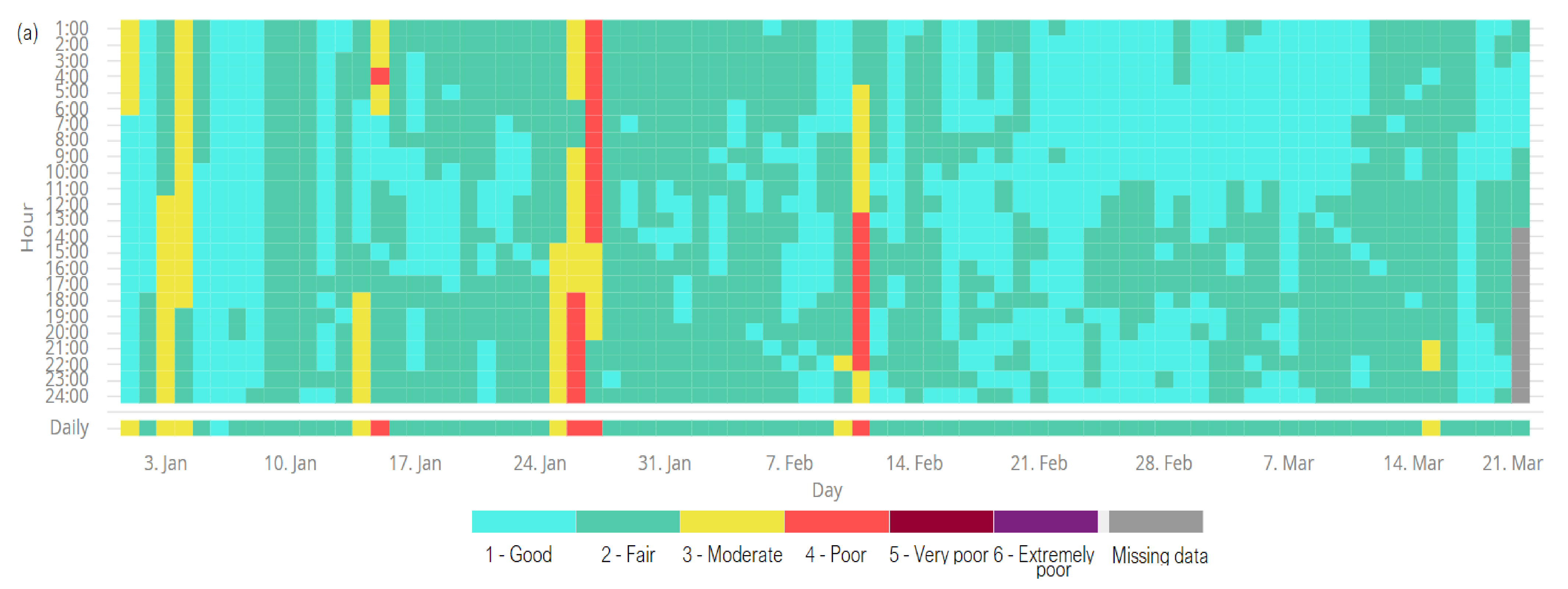
The specific air quality index, in short, “specific index”, is a system used for coding the recorded concentrations for each of the monitored pollutants (SO2, NO2, O3, PM2.5, and PM10) and is established for each of the automatic stations within the National Air Quality Monitoring Network as being the highest of the specific indices corresponding to the monitored pollutants. The general index and specific indices are represented by integers between 1 and 6, with each number corresponding to a color (1—good—turquoise, 2—acceptable—green, 3—moderate—yellow, 4—bad—red, 5—very bad—burgundy, 6—extremely bad—violet). The specific indices and the general index of the station are updated hourly [48]. For example, Figure 1 shows a recent map of the air quality in Romania.
The critical concentration levels established by Romanian law [47] for NOX/NO2 is as follows: 400 µg/m3alert threshold; 200 µg/m3 NO2—hourly limit value for human health protection; 40 µg/m3 NO2—the annual limit value for the protection of human health; and 30 µg/m3 NOx—annual critical level for vegetation protection.
The results of studies have shown that the average number of days on which there is good air quality in big cities in Romania (Bucharest [49], Timisoara [50,51,52], Cluj-Napoca [53], Constanta, and the surrounding area [54,55], etc.) has decreased year by year.
Since NO2 pollution in different European cities remains high (>40 µg/m3 is the maximum accepted annual mean concentration) and given its harmful effects on population health [14,46], continuous monitoring is required.
Understanding the existence of anomalies existence is becoming an important topic in the investigation of air quality. Anomalies are values in a data series that are unusual or dissimilar from the remaining data. They may be irregular items resulting from unusual or unexpected events, indicating abnormal behavior [56,57]. The analysis of anomalies is necessary for the detection of the source of their occurrence [57]. Hawkins et al. [58] stated that the values of series collected in polluted areas can behave as anomalies (outliers).
Despite the importance of the detection of outliers in atmospheric sciences, only a few articles, especially in the last years, have investigated this aspect and proposed new approaches for the better selection of such values [56,57,58,59,60].
In the above context, this study aimed to identify the anomalies in a nitrogen oxide series in Timisoara, one of Romania’s most prosperous industrial cities. The motivations for this study are as follows:
  • Only a few studies have been devoted to studying the existence of outliers in a pollutant series, with none of them using data collected in Romania.
  • Only a few articles have used hybrid approaches to model pollutant series, with most of them being based on atmospheric circulation models, not on the Box–Jenkins artificial neural network approach.
  • Very few studies have attempted to improve the quality of models after the removal of aberrant values from the time series.
Therefore, three models are proposed for a raw series including nitrogen oxides and ozone, and the series after the removal of outliers. Their performances are compared to determine the influence of the aberrant values on the models’ quality.

2. Materials and Methods

2.1. Data

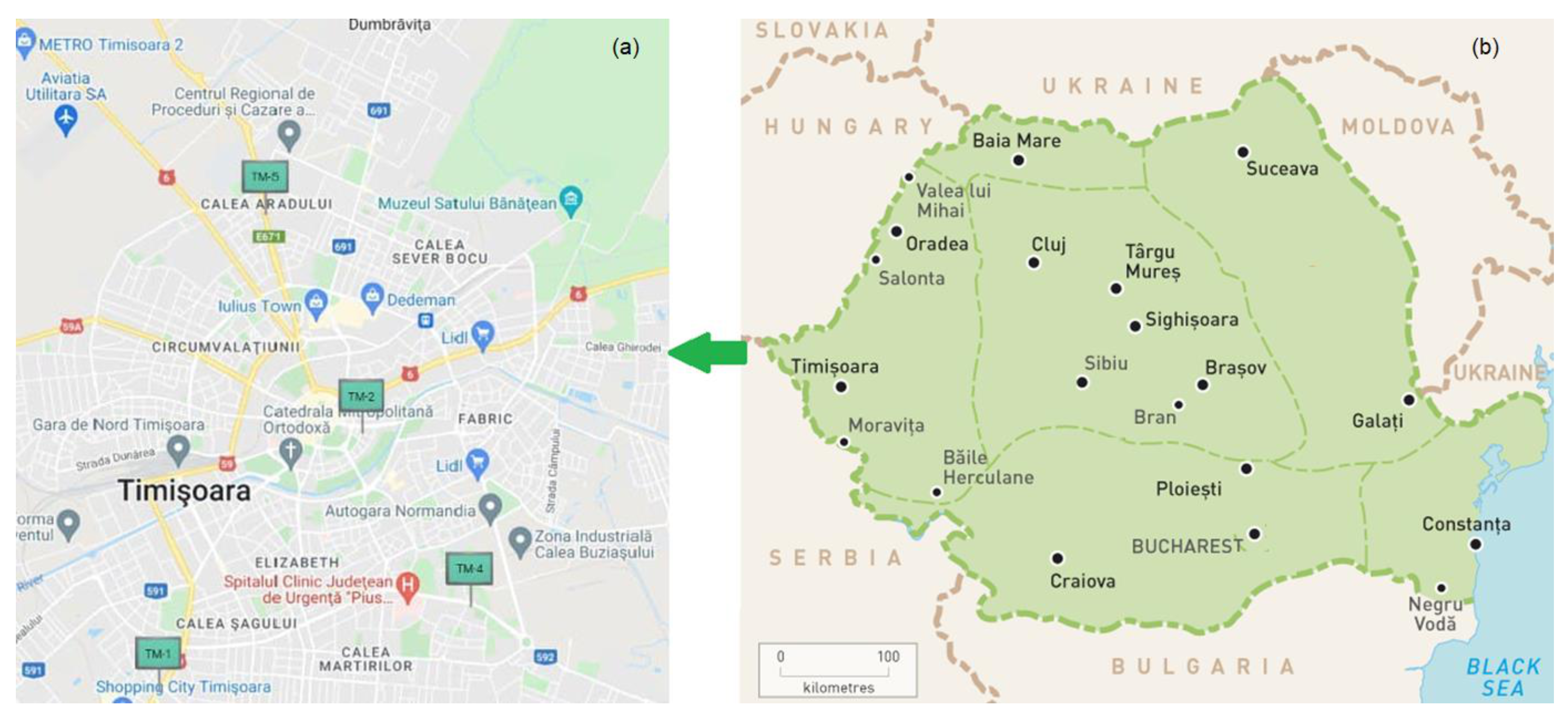
The geographical area of this study is Timiş county, located in the southwest Romania plain (Figure 2). The most important city in this county is Timișoara, situated at 45°44′ northern latitude and 21°13′ eastern longitude. It is one of the most prosperous economic and university cities. After 1990, transport, especially by cars, recorded an accelerated increase (reaching 1 car for every 2.66 inhabitants in 2017).
Therefore, the pollution produced by this sector has proportionally increased.
The climate is moderate continental, with winds blowing from west and north-west, and an annual precipitation of 650 L/m2. The atmospheric circulation favors the accumulation of pollutants emitted in industrial zones and car exhaust above the city.
Data (NO, NO2, and NOx and O3 concentrations) recorded at the monitoring station TM2 (C. D. Loga Blvd.—45°45′16.88″ N; 21°14′05.91″ E, 92 m altitude) were downloaded daily from the NAQMN website [15] during the period 1 January–8 June 2016. They formed complete sets (Figure 3) without gaps. It is noted that the highest values were recorded for the NOx series during the period March-April 2016 and for NO in the second half of May. The NO series exhibited the lowest variability. The existence of periods when the NOx concentrations were much higher than the sum of the NO and NO2 concentration is also noted, given that apart from NO and NO2, NOx incorporates other nitrogen oxide species that can accumulate in the atmosphere in periods of calm before participating in chemical reactions.
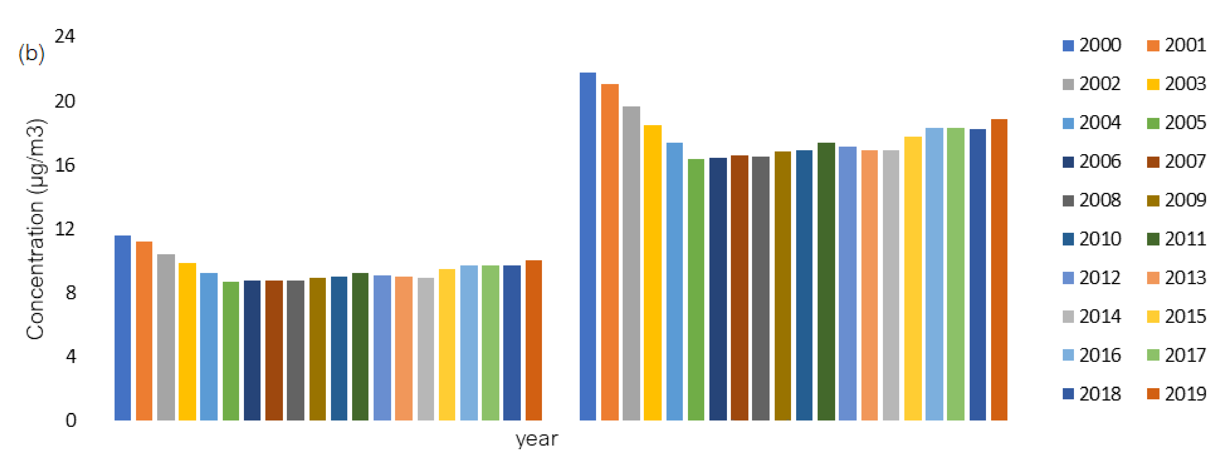
An example of the hourly air quality at the studied station during the period 1–21 March 2021 is presented in Figure 4a and the average annual concentration of NO2 in Timisoara during the period 2000–2019 is presented in Figure 4b.

2.2. Methodology

2.2.1. Statistical Analysis

The hourly data were processed to build the average data series, which was studied. The statistical analysis consisted of normality, homoskedasticity, autocorrelation, and stationarity tests, using the Shapiro–Wilk and Fligner–Killeen test, Levene test, autocorrelation function, and KPSS test, respectively. The Pettitt test was used to address the existence of a change point (in mean) [3].
Anomaly (aberrant) detection is used in many domains, such as manufacturing error detection, attack detection in cybersecurity, stroke recognition in EEG measurement, etc.
Anomalies are observations that deviate significantly from the expected behavior and cannot be categorized as noise or measurement error, and thus cannot be easily discarded [61]. In the case of anomalies, the unexpected event might be the study object.
Fox et al. [61] define two types of anomalies: type I, affecting a single instance; and type II, where the anomalous behavior extends in time.
Anomaly detection can be studied in both the univariate and multivariate time domains, with the latter possibly implying multiple dimensions that display anomalies simultaneously or even waterfall effects. Here, we focused on the univariate case.
Most techniques used for anomaly detection in time series consider the time aspect, either in the vicinity or globally, using the entire data series to mark the anomalies. Four such methods were applied in this study [62]. One of the most popular, called the IQR method, considers values outside the interval (Q1 − 1.5 IQR, Q3 + 1.5 IQR) as anomalies (Q1 is the first quartile, Q3 is the third quartile, and IQR is the interquartile range). Sometimes, the term 1.5 is replaced by 3.
The second method employed in this study is isolation forest (IF) [63,64,65]. It relies on the concept of isolating unusual instances, as opposed to determining the properties of normal samples and then examining non-matching patterns. It achieves anomaly detection by building isolation trees (ITs), where anomalies are often represented as existing closer to the root of the IT, rather than higher at the leaves, where regular data points are found.
To build the trees, IF generates recursive partitioning of the dataset (Figure 5) by randomly selecting a dimension in the dataset, followed by a recursive split of the specific dimension anywhere between the minimum and maximum value of the remaining set.
A path length of a point x, PL(x), is computed as the number of edges x that traverse an isolation tree from the root node until the traversal is terminated at an external node.
Computing the path length means to count the number of partitioning steps required to isolate a data point. The lower the path length or tree height value, the higher the probability of a specific instance being an anomaly.
The average path lengths for instances are then used to evaluate the probabilities of data points showing anomalous behavior.
The application of IF for anomaly detection has two main steps:
  • Building and training the isolation trees.
  • Assigning anomaly scores to data points based on PL by computing the tree height length as binary search trees.
The anomaly score s of an instance x is defined as:
s x ,   n = 2 E L x / c n ,
where E(L(x)) is the average of L(x) from a collection of isolation trees, and c(n) is the average of L(n) given n instances.
3.
Using the anomaly scores, the following decision is made:
(a)
If instances have an s value that is much smaller than 0.5, then they are considered normal instances;
(b)
If all the instances have s ≈ 0.5, then the entire sample does not have any distinct anomaly;
(c)
Instances with an s value larger than 0.5 are marked as anomalies [63].
While IQR and IF detect global outliers, LOF mainly identifies local outliers [42]. The decision regarding whether an outlier is local is made based on an evaluation of the associated probability, determined by the k-nearest neighbors (kNN) method [66].
To determine if a point p in a study set is an outlier, the following operations are performed in LOF [67] for p: (a) computation of the k-distance; (b) computation of the kNN; (c) calculation of the local reachability density; and (d) detection of the LOF score. Point p is classified as an outlier by comparing the score with a given threshold.
The last method utilized to detect both types of anomalies—local and global—in the data series is the generalized extreme studentized deviate test (GESD) [68]. Its stages are as follows:
  • Analyze the existence of periodicity in the data series;
  • Divide the series into non-overlapping intervals Iw;
  • For each interval:
    Determine the seasonal compound (if it exists);
    Compute the median;
    Extract the residual, as the difference between the values of the series, the median, and the seasonal component;
    Run the ESD algorithm (with the median and mean absolute error in the computation of the test statistics) [69].
  • Return the outliers obtained from the previous stage.
The advantage of this technique is that it can be used even if the timestamps are unknown.
The correlation between the four series and the series anomalies, respectively, is addressed by computing the correlation coefficients. In the case of low correlations, models were built only for the individual series.

2.2.2. Modeling

This work emphasizes how aberrant values (anomalies) influence the quality of models built using raw series and after their removal. ARIMA, GRNN, and hybrid ARIMA-GRNN models were built for the raw series and the series obtained after removing the aberrant values.
A time process ( X t , tZ) is stationary if it satisfies the following conditions:
  • t Z ,   M X t 2 < + ;
  • t Z ,   M X t < + and is invariant in time (M denotes the expectation);
  • t , h Z ,   Cov X t ,   X t + h = γ h (i.e., the covariance of X t and X t + h depends only on the lag h).
Let us denote the d-the order difference of X t by Δ d X t , where B is the backshift operator.
A time process (Xt; tZ) is called an autoregressive integrated moving average process ARIMA(p,d,q) if:
Φ B Δ d X t = Θ B ε t ,
where Φ and Θ are respectively polynomials of p and q orders with roots higher than 1, respectively, and ( ε t , tZ) is white noise [70].
Among two valid models, the best one is selected based on the Akaike criteria. The lower the AIC value, the better the model is [70].
An ARIMA(p, q) process is a particular case of ARIMA, with d = 0.
Generally, a stationary process can be approximated by an ARMA(p, q) model.
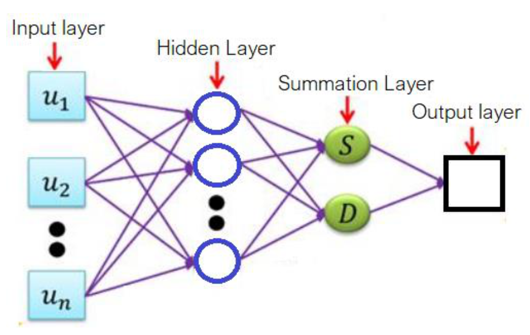
The generalized regression neural network belongs to the group probabilistic neural networks. It is composed of four layers (Figure 6) [71].
The first one—input—contains the series values X = ( x 1 ,   ,   x n ) . The second one—hidden—is composed of neurons that apply a kernel function to the distances between the training data and the prediction point. In this process, σ values are employed to compute the radius of influence. The best σ is determined when the network is trained to control the distributions of the kernel function. In this study, the Gaussian kernel was utilized, and the gradient algorithm was employed to estimate the best σ [71].
In this study, the interval 0.0001–10 was used to search for σ values in.
The number of neurons in the hidden layer after training is the same as the number of training samples involved in the modeling. The unnecessary neurons are removed based on the error minimization criterion during an optimization process [71,72].
The summation layer is composed of two neurons (D- and S-) that sum up the values collected from the previous layer. The only difference between them is that the D-summation neuron computes a weighted sum of the values resulting from the hidden layer [72].
The last layer (output) provides the ratios between the corresponding values from the D- and S- summation neurons.
To perform the modeling, the series was divided into a ratio training:test = 80:20, with the first part used for training, and the second part for testing. The number of iterations was fixed at 5000 (maximum) and 1000 (without improvement). The regressors were considered as lagged variables, with lags between 1 and 6. The algorithm was run with different regressors, and the best result was kept. The correlation between the actual and predicted values (rap), mean standard error (MSE), mean absolute error (MAE), mean absolute percentage error (MAPE), and R2 were employed.
In the hybrid ARIMA–GRNN procedure, an ARIMA model was first built for the data series, and then the residual was modeled using GRNN. The same setting that was used in the GRNN algorithm for the data series was kept when running GRNN for the residuals in the ARIMA model.
The ability to capture nonlinearities, the use of nonparametric regression, and learning without backpropagation is recommended regarding GRNN to solve classification, regression, and forecast problems involving continuous variables [71,72]. These characteristics improve ARIMA’s capabilities to model processes with phenomena with high linear dynamics.
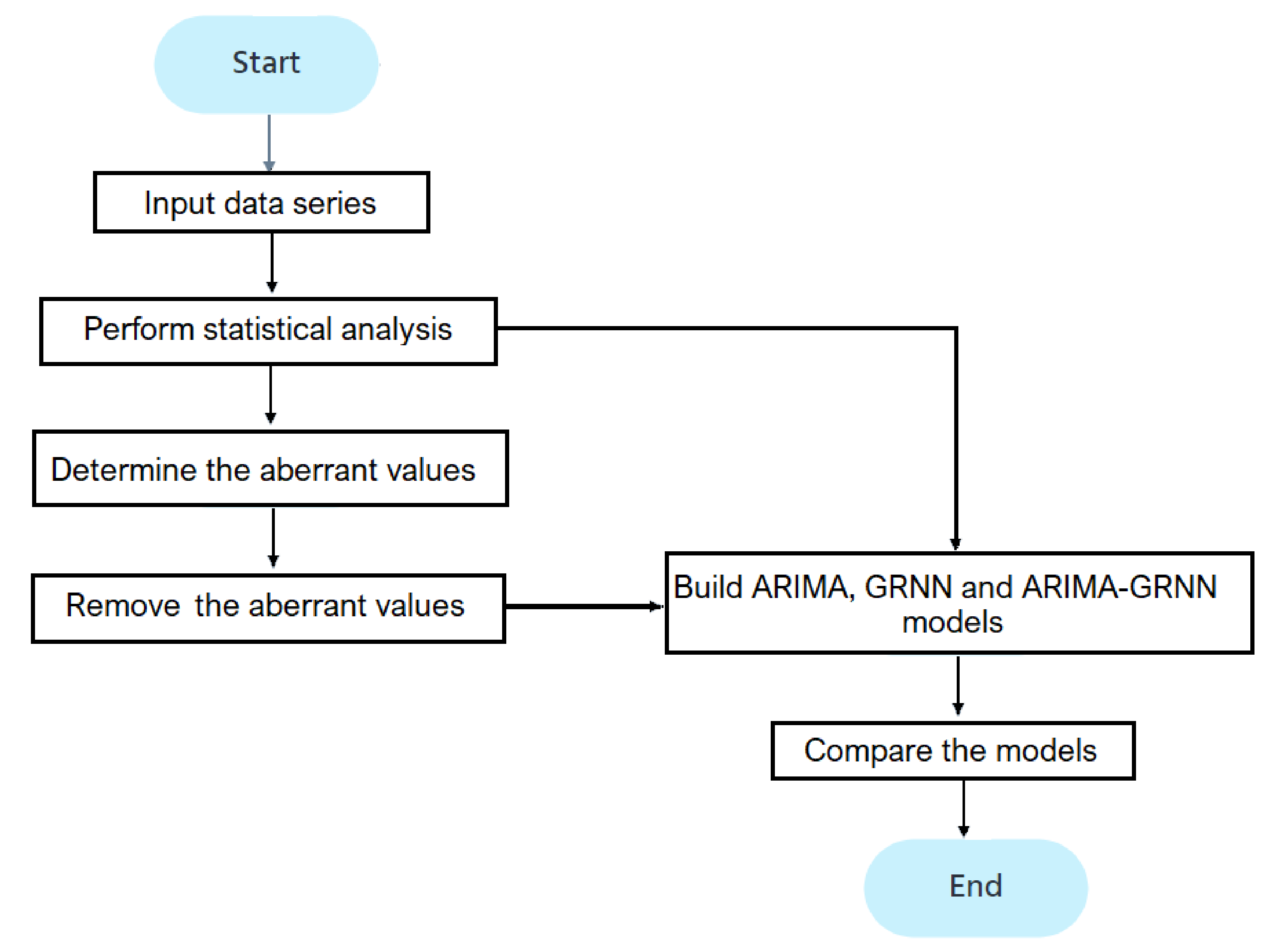
Figure 7 shows a flowchart of the study.

3. Results and Discussion

3.1. Results of the Statistical Analysis and the Anomaly Detection

The basic statistics of the average data series are presented in Table 1.
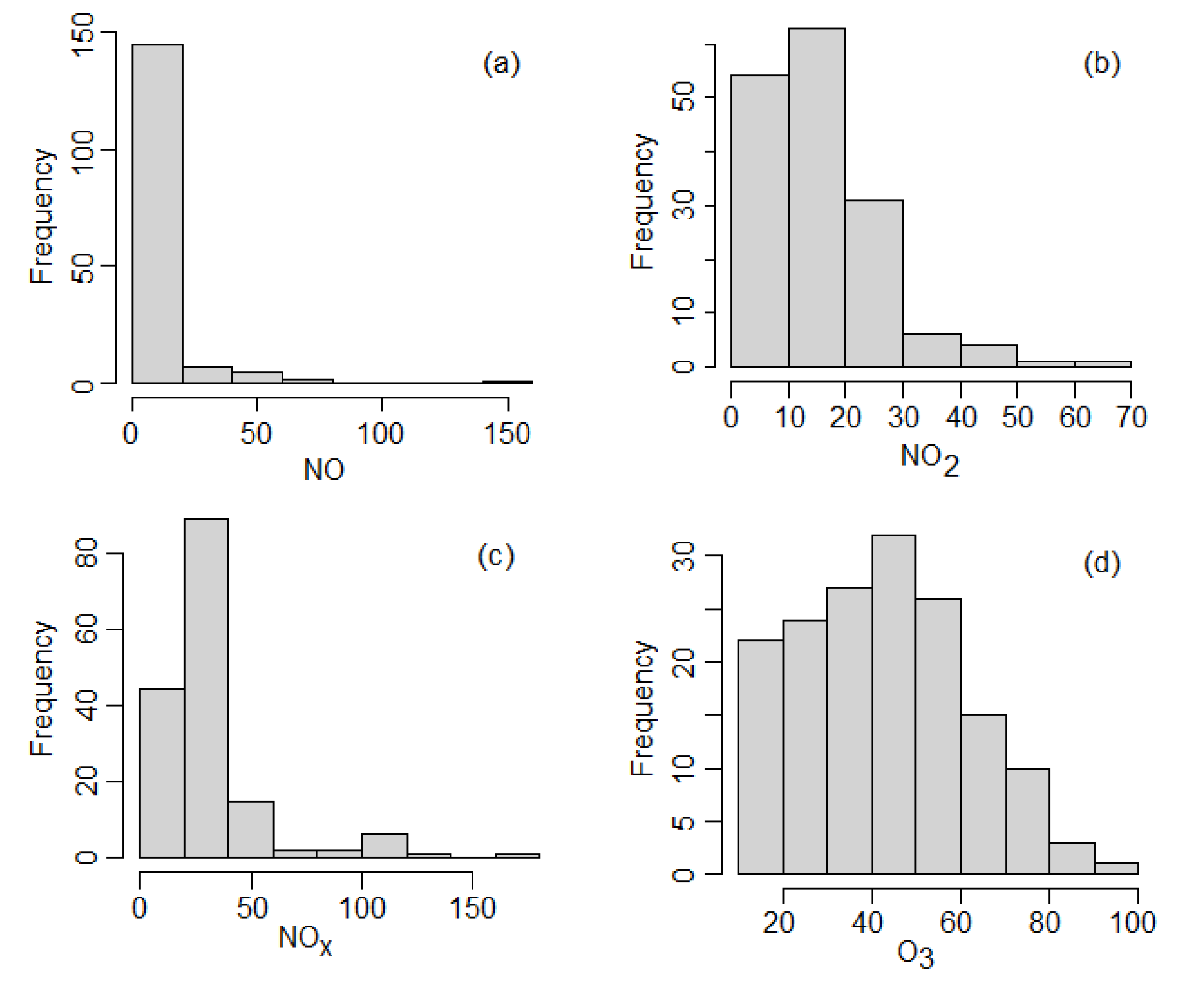
The NO and NOx series display a very high range while the NO2 and O3 ranges are more than twofold lower compared to those of the first two series. The lowest average corresponds to NO. It is very small compared to the maximum, indicating that most series values are closer to the minimum than to the maximum. NOx showed low average values compared to the maximum for. All series had moderate standard deviations (stdev) and coefficient of variations, indicating a moderate dispersion of the data series around the average values. The series are right-skewed (skew >0), which is confirmed by the histograms shown in Figure 8. The kurtosis coefficient indicates leptokurtic distributions for all but the O3 series (which is platykurtic).
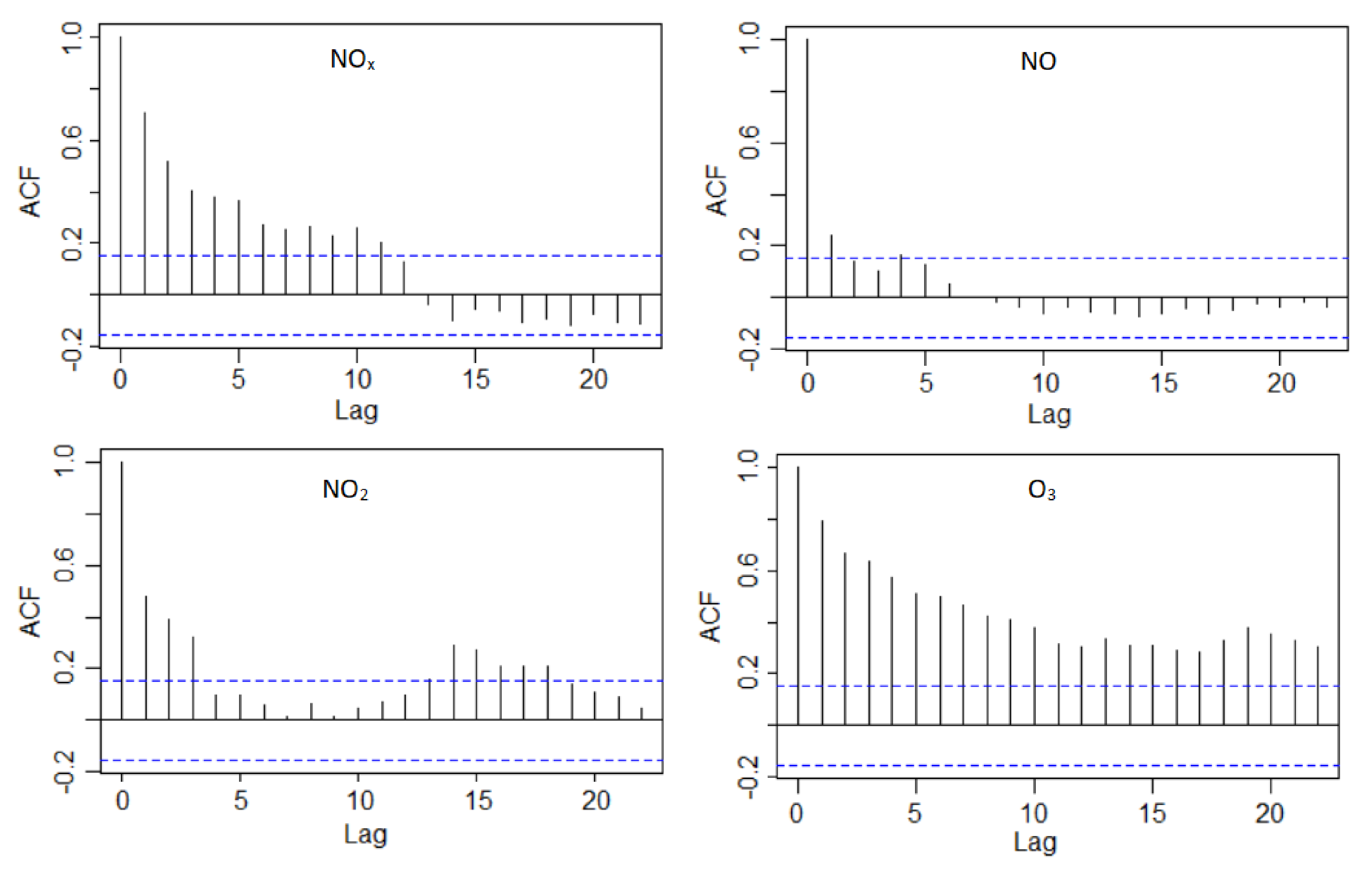
The normality and randomness hypotheses were rejected at the significance level of 5%. The homoscedasticity hypothesis was rejected for the NOx series only (the p-value computed in the Levene test is 0.022). Figure 9 shows the presence of at least first-order autocorrelation for all the data series.
The KPSS test rejected hypothesis of level-stationarity for NO2 and O3, and trend-stationarity for NOx and O3.
After applying the change point test, the hypothesis that there is no change point could not be rejected for all the series. Two subseries were detected for each series. The change point and the subseries averages are presented as follows, where mean 1 is the average of the subseries containing the values before the change point, and mean 2 is the average of the subseries formed by the values after the change point:
  • For NO: the change point is the 98th value, mean 1 = 12.611, mean 2 = 5.659;
  • For NO2: the change point is the 92nd value, mean 1 = 19.454, mean 2 = 10.544;
  • For NOX: the change point is the 87th value, mean 1 = 40.426, mean 2 = 23.348;
  • For O3: the change point is the 55th value, mean 1 = 25.554, mean 2 = 51.182.
So, the series presents high variability. The higher the variation is, the more difficult it is to find a good model.
The IQR method with a factor of 1.5 (and 3) detected the values situated outside the following intervals as outliers:
  • [−7.5305, 20.65750] and [−18.101, 31.228] for NO;
  • [−10.1676, 39.0445] and [−28.622, 57.499] for NO2;
  • [−3.825, 57.975] and [−27, 81.15] for NO3;
  • [−14.195, 97.205] and [−55.97, 148.98] for O3.
This study was performed in the first case because the use of three reduces the domain of the anomalies. Therefore, based on this criterion, values recorded on the following days were outliers:
  • 4, 5, and 9 February; 23–29 March; and 21 May for NO;
  • 11 and 25 February; 7–11 and 23, 28, and 29 March; and 27, 29, and 30 May for NO2;
  • 1, 9–13, 16, 17, and 19–22 March; and 7 May for NOx;
  • 6, 7, 13, and 29 January; 5 February; 5 and 28 March; 1, 2, 6, 8, 12, 14, 15, 18, 21, and 22 April; and 7 June for O3.
The NO, NO2, and NOx series, with the anomalies determined by IF, are presented in Figure 10. The aberrant values are mostly very high, especially for NO and NOx.
IF provided more anomalies in comparison to IQR, but most of the aberrant values detected by the IQR method were also identified by IF. The aberrant values identified by IF included the values recorded on the following days:
  • 1–10, 17, 18, and 22 January; 2, 3, 11, 25, 28, and 29 February; 7–11 and 23, 28, and 29 March; 27 April; 19 and 27–30 May; and 1, 3, and 6–8 June for NO;
  • 11 and 25 February; 23 March; 27, 29, and 30 May; and 1, 6, and 9 June for NO2;
  • 1–5, 9, 13, 17, 22, and 29 January; 4–6, and 29 February; 1, 9–13, and 16–22 March; 7 and 19 May; and 4–8 June for NOx;
  • 1–7, 9, 13, 17, 18, 28, and 29 January; 1, 5–7, 13, 15, and 23 February; 5, 6, 22, and 28 March; 1, 2, 6, 15, 18, 21, 22, and 28 April; 4, 30, and 31 May; and 1–8 June for O3.
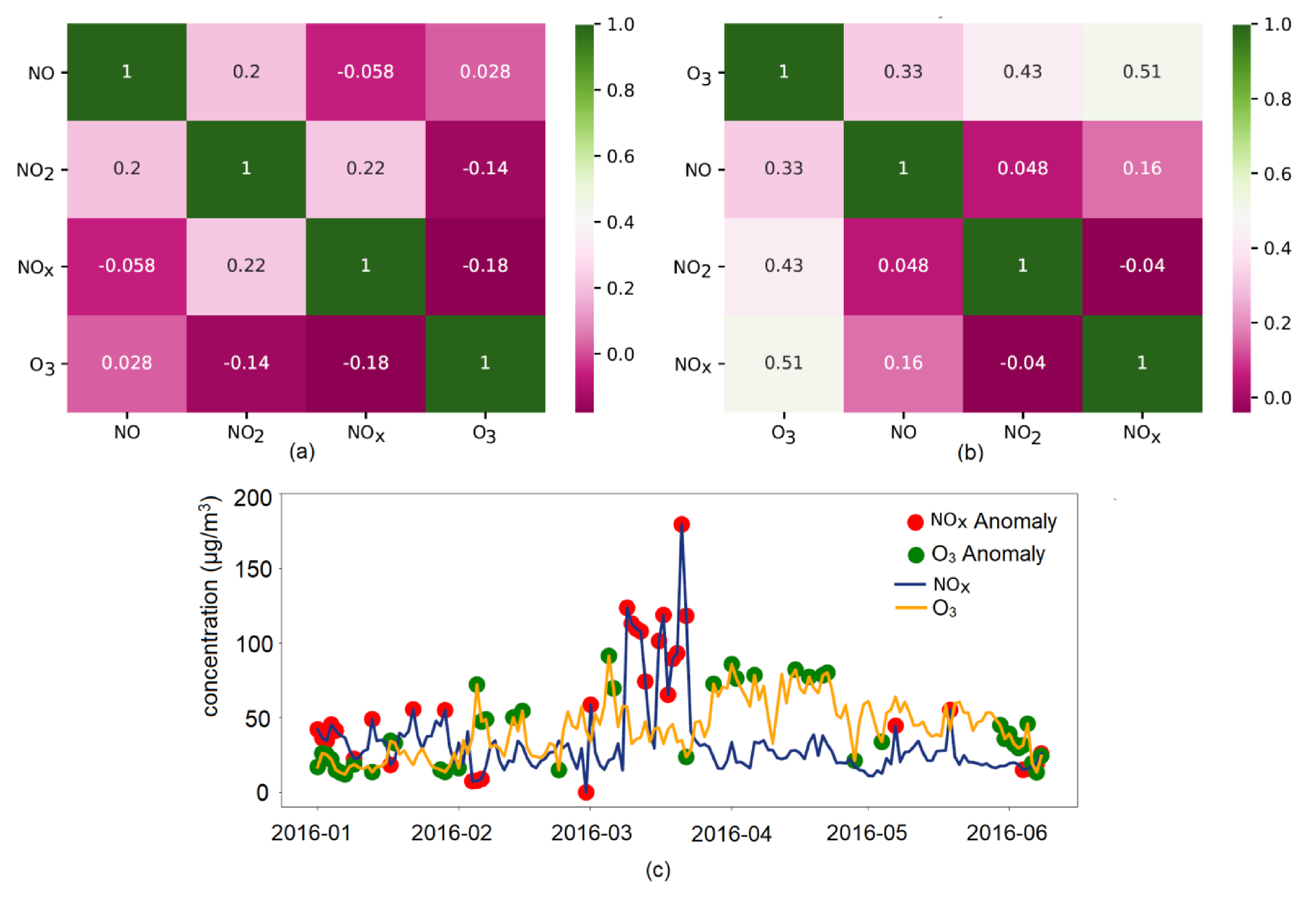
Given the common origin of nitrogen oxides and the chemical reactions that occur when O3 is present, as explained in the introduction, the correlations between the concentrations of the studied pollutants were investigated. Figure 11 presents (a) the correlations between the NO, NO2, NOx, and O3 series and (b) the correlations between the series of anomalies detected by IF. While no significant correlations between the pollutant series were detected (the correlation coefficients range from −0.18 to 0.22), the highest correlations were identified between the O3 anomalies and NOx anomalies (NO2 and NO anomalies, respectively), with a value of 0.51 (0.43 and 0.33, respectively). Still, these values do not show a strong correlation between the aberrant series.
Figure 11c depicts the NOx and O3 series, and their anomalies.
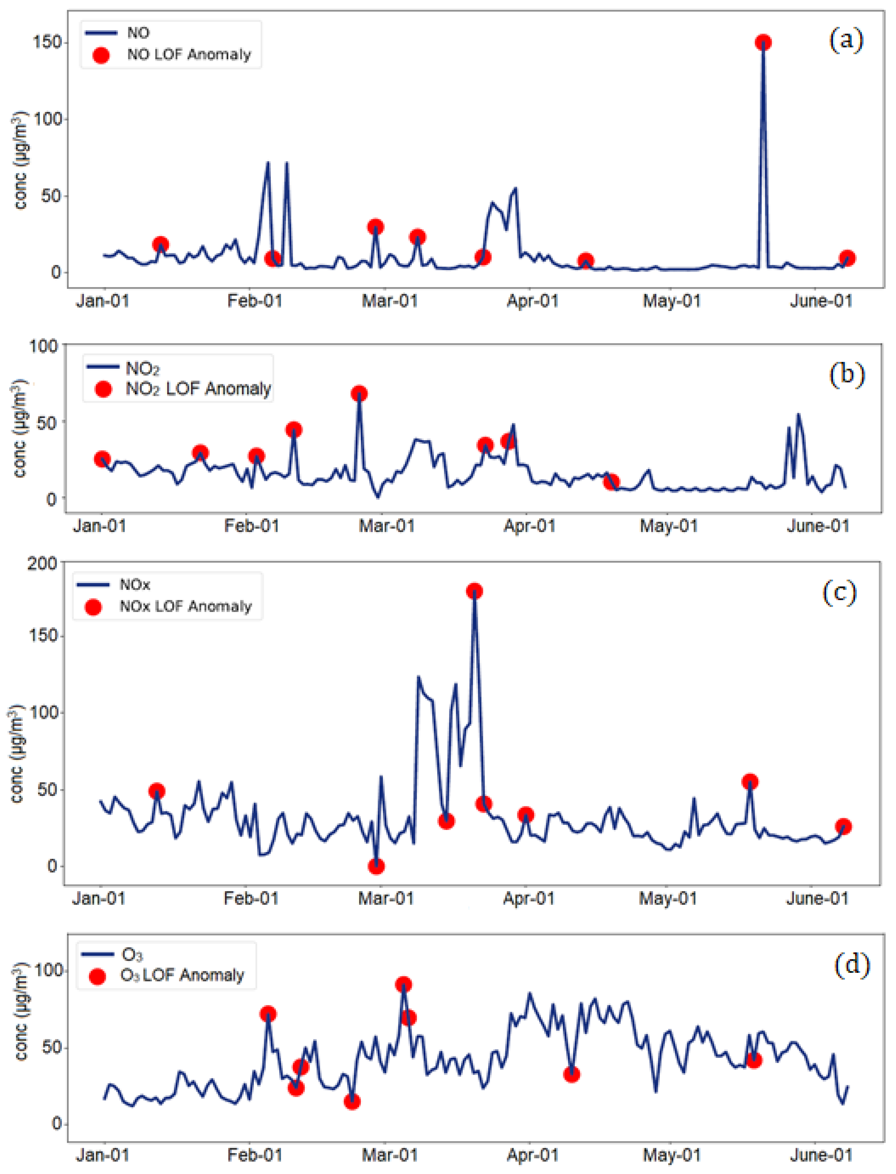
Figure 12 displays the series with the highlighted anomalies determined by LOF. Notice that the IF approach provided a higher number of anomalies than LOF. This result is due to the LOF algorithm only considering neighboring values rather than the entire series. Five common anomalies are provided by IF and LOF for NO, NOx, and O3, and seven for NO2. The correlation between the series anomalies is close to zero. Figure 13 shows the anomalies detected by GESD. This algorithm did not find any anomalies in the O3 series, 3 for NO2 (25 February, 29 March, and 29 May), and 11 for NOx (9–13 and 16–22 March). The outliers detected by this algorithm and IQR for NO are the same. Since no significant correlation between the data series was found, we did not search for a regression model, linking different variables. The next section contains the results of modeling the data series before and after the removal of the anomalies.

3.2. Models for the NO2 Series

As presented in the previous section, the NO2 series is not Gaussian. Since the normality of the series was achieved through a Box–Cox transformation with the parameter λ = 0.130 , the series was firstly normalized and then stationarized by taking the first-order difference. Using the Akaike criterion and the capabilities of R software, the best ARIMA model for the transformed series (denoted NO2BC) was the ARMA(1,1) type, with an autoregressive coefficient AR1 = 0.4728, moving average coefficient MA1 = −0.9069, and corresponding standard errors of the coefficients of 0.0973 and 0.0505. The values of the goodness of fit indicators for the model are a mean error (ME) = 0.0380, RMSE = 0.6488, MAE = 0.4543,—mean percentage error (MPE) = 0.268, and MAPE = 15.8283.
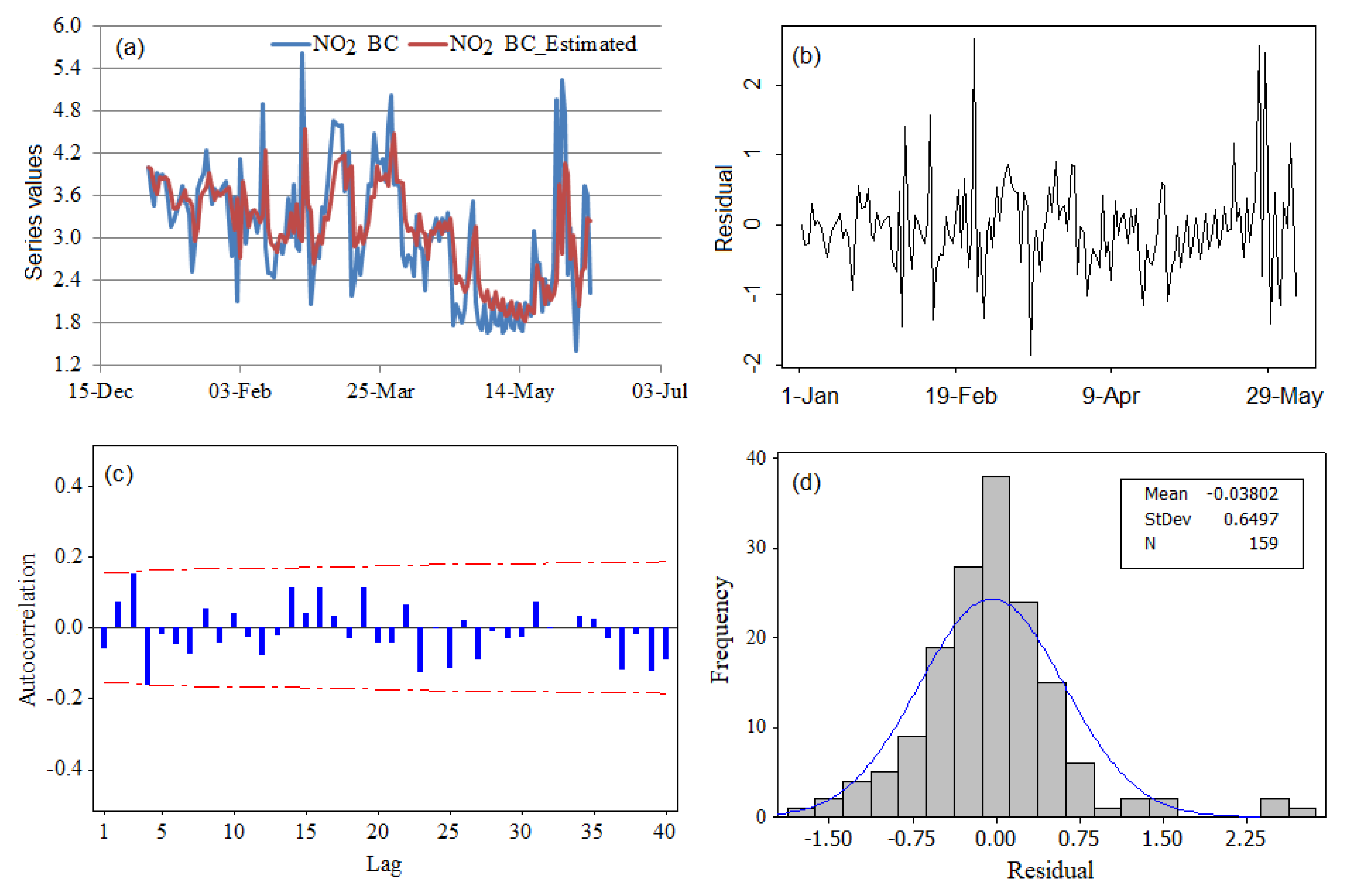
Figure 14a shows the NO2BC series and the estimated one, whereas Figure 14b–d present the residual series, the residual autocorrelation function, and its histogram.
Figure 14a shows good concordance between the recorded values (blue) and those estimated by the model (red). Figure 14c reveals no residual autocorrelation. The histogram (d) shows a mean value of the residuals of about zero and an almost symmetrical distribution of the residuals. The normality test of the residual series could not reject the normality hypothesis while the Levene test rejected the homoskedasticity one. Therefore, the residuals do not form white noise; so, the model could not be validated from a statistical viewpoint.
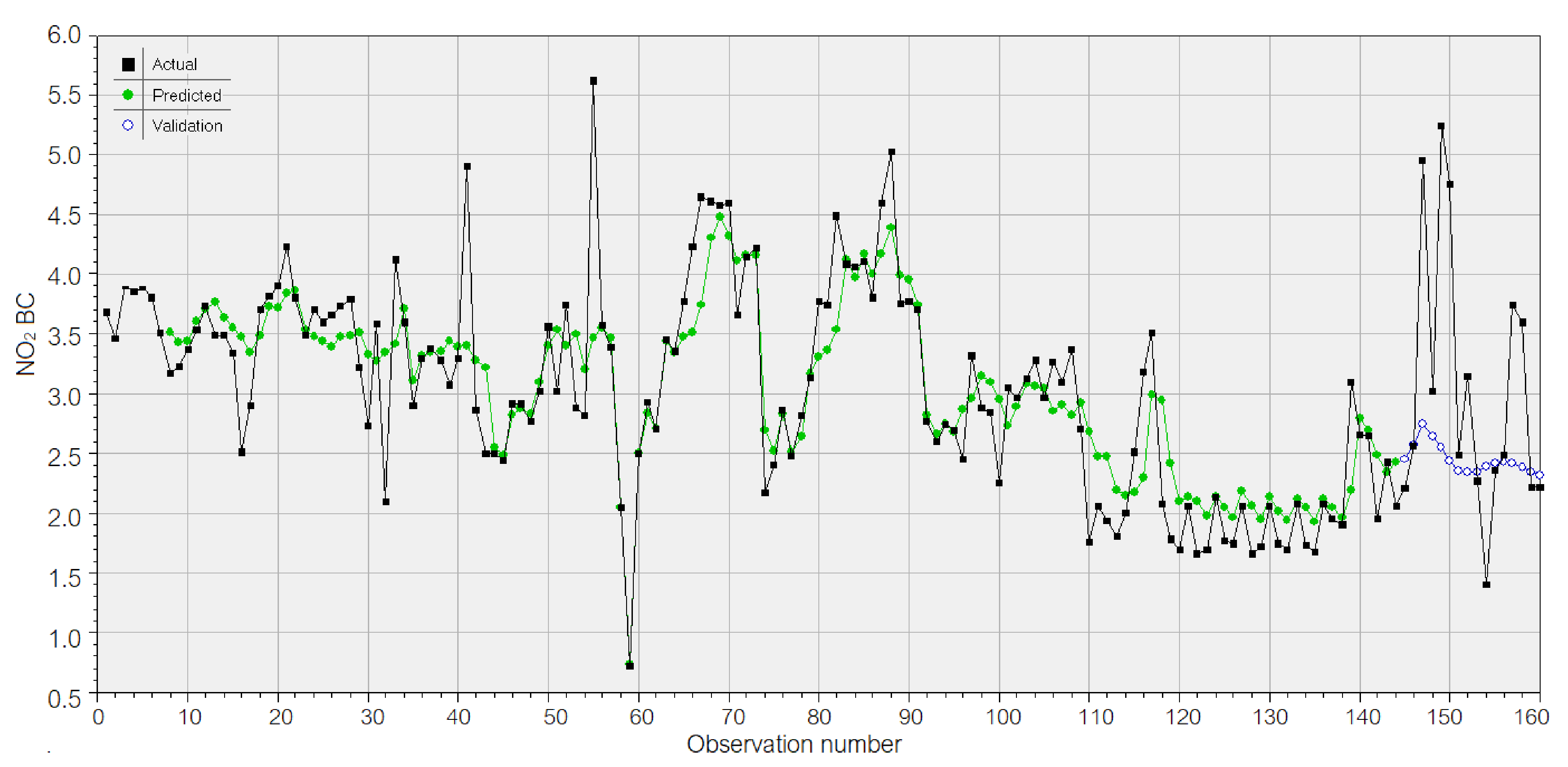
Figure 15 presents the chart of the GRNN model for the normalized NO2 BC series after removing the exponential trend with the following equation:
(NO2 BC)t = 5.8286 − 2.1721 × exp(0.00296t),
where (NO2 BC)t is the concentration of the value of the NO2 BC series at the moment t.
The model could learn the data well since the model’s total variance on the training set is 76.135%, the correlation between the actual and predicted values is 0.8778, MSE = 0.177, MAE = 0.2839, and MAPE = 9.9786. Still, on the test set, the results are worse. For example, MSE = 1.5101, MAE = 0.8175, and rap = 0.4482.
Given that the ARIMA model could not be validated and the relative inability of GRNN to apply what was learnt in the training phase in the test, we searched for a hybrid model that could fit the data better and benefit from the ability of ARIMA to capture the linear behavior and the ability of GRNN to catch the nonlinear one. The raw series was considered to fit the ARIMA model, and then the residual series was subjected to GRNN modeling.
The best hybrid approach ARIMA-GRNN obtained for the NO2 series is described as follows (Figure 16):
  • An ARIMA(2,1,1), with:
    The autoregressive and moving average coefficients (and standard deviations) AR1 = 0.3584 (0.0834), AR2 = 0.1811 (0.0826), and MA1 = −0.9677 (0.0294);
    MSE = 81.4417, MAE = 5.6679, the first-order residual autocorrelation = 0.97973;
    AIC = 1161;
    MAPE could not be computed (there is a value equal to 0);
  • The GRNN model for the residual, with a lagged 1 variable as the regressor, and:
    On the training set: R2 = 99.635%, rap = 0.998178, MSE = 0.2562, MAE = 0.1112, MAPE = 27.4644.
    On the test set: R2 = 0.0635%, rap = 0.0578, MSE = 1222.97, MAE = 5.239, MAPE = 84.36.
Therefore, the GRNN model learnt the data well but could not use what it learnt for forecasting. Still, the new residuals are Gaussian.
Since the global anomalies were of interest, comparisons of the results provided by IQR, GESD, and IF were made to identify the values that were removed before the modeling. In the first stage, the common values provided by these methods were selected and removed from the data series. IQR was applied again to the new series in the second stage. Finally, the common values provided by IF remained after the first stage, and those from the second stage were removed. This procedure was chosen considering most anomalies detected.
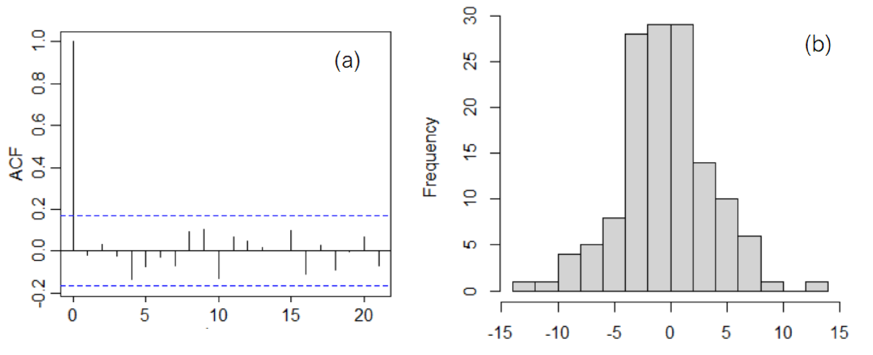
The ARIMA model for the series without aberrant values (called NO2New) was an ARIMA(1,1,1) type, with the following autoregressive and moving average coefficients (with the corresponding standard errors in brackets): AR1 = 0.4671 (0.0955) and MA1 = −0.9083 (0.0438), MSE = 15.95, MAE = 3.0694, MAPE = 30.76299, and AIC = 770.53. The residual variance in the ARIMA(1,1,1) model is 15.8890. The residuals’ correlogram and their histogram (Figure 17) indicate that this series is not correlated and is Gaussian (confirmed by the Anderson–Darling test, where the p-value is 0.1269). The heteroskedasticity hypothesis was also rejected. Therefore, from a statistical viewpoint, the ARIMA(1,1,1) model is correct.
The forecast for the next 48 moments based on the above model is shown in Figure 18 (the right-hand side), in blue, together with the confidence intervals at the confidence levels of 95% and 90% (different nuances of grey). The shape of the forecast series is not similar to that of the actual one. Its trend becomes almost linear after eight-time moments. Therefore, the model cannot be utilized in a future forecast, even if it was statistically validated.
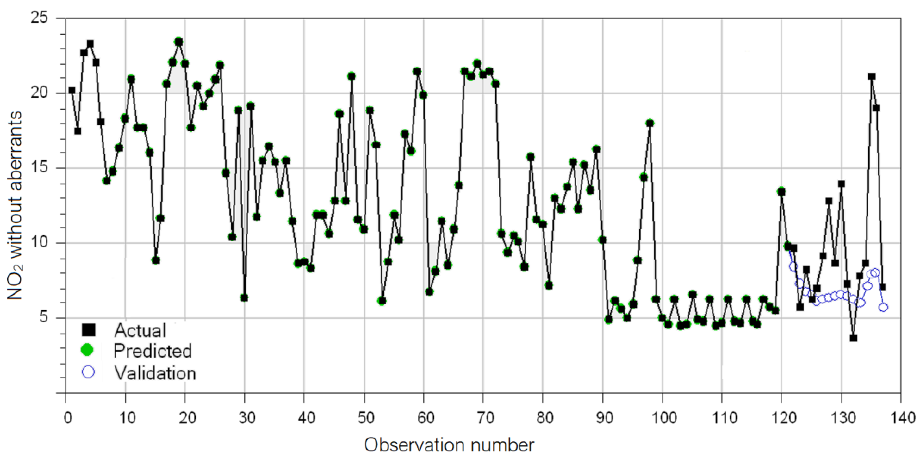
The GRNN model for NO2New is presented in Figure 19. The model learnt the data in the training set well (R2 = 0.996). On the test set, MSE = 25.5047, MAE = 3.1555, and MAPE = 27.9311, but R2 = 0.473 is not close to 1.
After comparing the GRNN performances on the initial series and that without aberrant values on the test set, the results of the last series are better. Still, the model should be improved because the blue dots—representing the computed values on the test set (validation in Figure 19) are not close enough to the recorded values, which were represented by the black line.
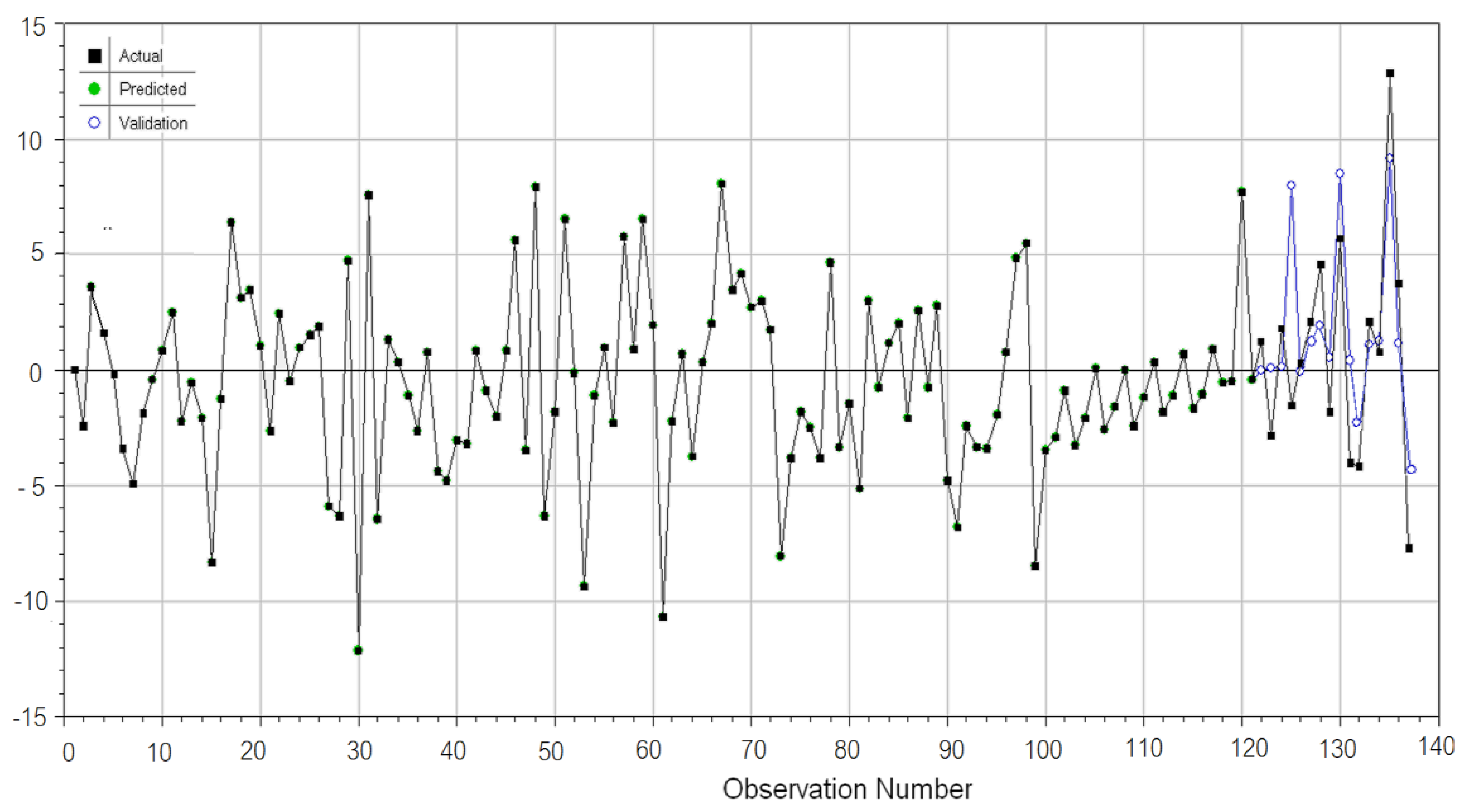
The hybrid ARIMA–GRNN model was built using the above ARIMA(1,1,1), whose residuals were modeled by GRNN (Figure 20).
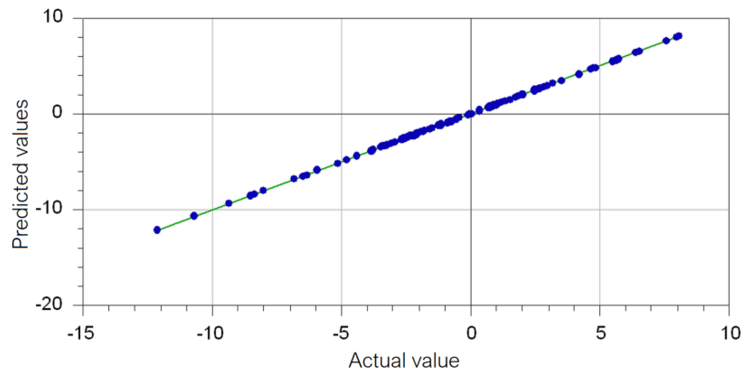
The neural network learnt the data well. Indeed, on the left-hand side of Figure 20, the actual values and the computed ones (called predicted) are practically superposed on each other (the black and the green lines). It also performed well on the test set. On the right-hand side of Figure 20, the recorded values (black) and computed values (blue) are close. To confirm the model’s goodness, Figure 21 displays the actual vs. predicted values in the residual modeling. The dots built by pairs of actual and predicted values of residuals are displayed along the diagonal (representing the ideal case of perfect superposition between the actual and computed values), indicating that the ARIMA-GRNN model performs very well. Therefore, the best model for the series without aberrant values is the ARIMA(1,1,1)–GRNN model.
Since similar results were obtained for the NO and NOx series, the authors did not repeat the entire procedure.

3.3. Models for the O3 Series

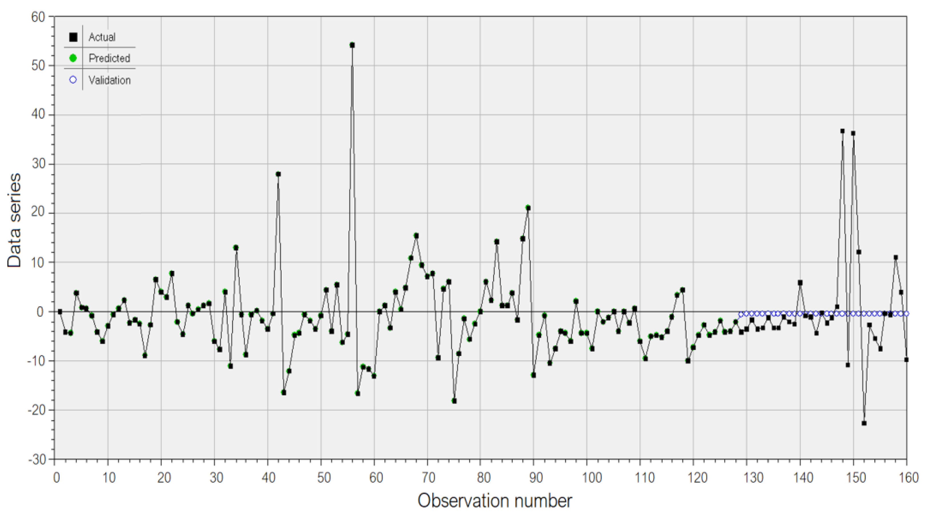
The same approach was followed to build models for the O3 series. Given that high O3 concentrations may negatively impact human health, a good forecast can provide information for early warning. The first approach provided an ARIMA(0,1,2) model for the raw data series. The series had to be stationarized before modeling (the degree of differentiation being 1). The moving average coefficients (with the standard errors in the brackets) are MA1 = −0.2971 (0.0789) and MA2 = −0.295(0.0884). The goodness of fit indicators are MSE = 69.72703, MAE = −5.392056, and MAPE = 21.79388. The MSE value is high due to the high variation in the errors. Despite their randomness, the residuals in the ARIMA(0,1,2) did not form white noise because they are not Gaussian (the p-value in the Anderson–Darling test is 0.0055 < 0.005) or homoskedastic. Figure 22 displays the residuals in the ARIMA(0,1,2) model for O3, their histogram, and the correlogram. The residuals chart in Figure 22 confirms the existence of high residual values. Since the model could not be validated, its improvement was necessary.
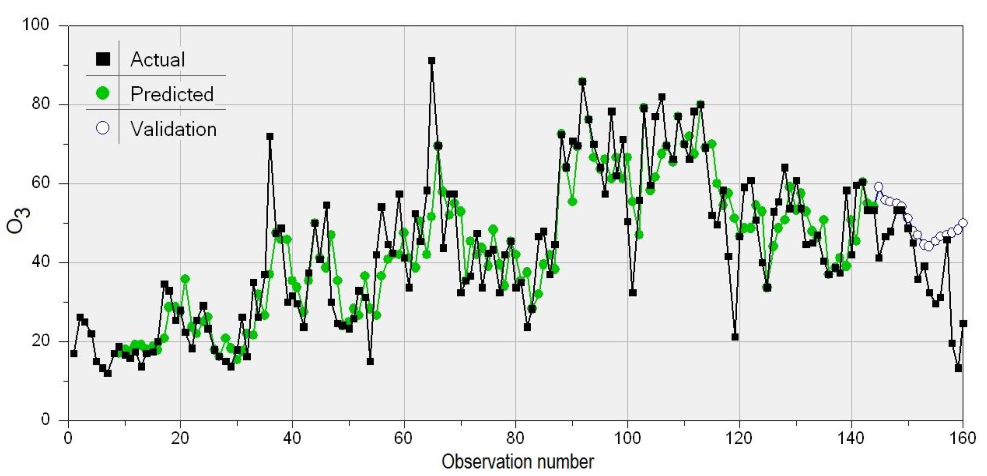
The neural-network approach provided a GRNN model (Figure 23) that learnt the data well but did not perform well on the test set. For example, on the training set, the correlation between the actual and predicted values is 0.8634 while on the test set, it is only 0.5282. On the test set, the computed values (represented by blue circles) do not have the same pattern as the recorded data (the black line).
The hybrid ARIMA-GRNN provided R2 = 99.681%, correlation between actual and computed values of 0.9984, MSE = 0.3965, MAE = 0.0606, and MAPE = 38.64744 on the training set. Still, the hybrid model did not perform well on the test set, since R2 = 5.898%, and the correlation between the actual and computed values = 0.333, so it cannot be used for prediction.
After removing the aberrant values from the O3 series, and performing the Mann–Kendall test [73], the hypothesis that there is no monotonic trend was rejected. Using the nonparametric method of Sen [74], it was found that the series presents an increasing trend, with a slope of 0.310673. The KPSS test revealed nonstationarity in the level of this series. It was found that the best model was ARIMA(0,1,0) with a drift of 0.310673 (the same as the slope). The goodness of fit indicators showed very low residual values (RMSE = 0.00022, MAE = 0.00233, MAPE = 0.000844), with no residual correlation. Given the model’s quality, it is not necessary to improve it.
From this model, it was found that the O3 series had an increasing trend over the study period, which must be observed in the future, since the O3 concentration may reach a level that is dangerous for the population.

4. Conclusions

The detection of aberrant values in time series has been a problem of interest for a long time, given that their presence may influence the modeling results. Moreover, forecasting based on derived models may be significantly biased by the existence of aberrant values. Therefore, this study investigated the influence of the presence of anomalies on a series of nitrogen oxide concentrations.
Given that some methodologies are used to search for different kinds of anomalies (local or global), first, the results provided by LOF, IQR, IF, and GESD were compared. Since the focus was placed on global aberrant values, their selection was made before using the last three algorithms for modeling.
Three models were built for each NO2 raw series and after the removal of anomalies: –ARIMA, GRNN, and a hybrid GRNN-ARIMA.
In the case of the NO2 series, the building of three models was necessary to improve the initial model, even in the absence of anomalies. This was motivated by the following reasons. An ARIMA model, for example, is not necessarily the best choice, given that the residual must be white noise (a fact that is not always true). A GRNN model is not appropriate because the R2 value or the correlation between the actual and predicted values is not very high on both the training and test sets. The selection of the regressors in the artificial intelligence-based approaches is not obvious. Their selection and number are essential for determining the best model. Even in the absence of outliers, improvement of the model is necessary to obtain a good forecast in the next stage. From this point of view, the best model is one that provides the best forecast.
It was shown that the removal of anomalies resulted in better models than when they were present. The ARIMA model for the raw data series could not be statistically validated whereas, for the series without anomalies, it was correct from a statistical viewpoint. The hybrid approach was also better than the ARIMA and GRNN on both NO2 series.
The hybrid approach provided the best model for the O3 raw series. After the removal of aberrant values, the ARMA(0,1,0) with drift provided the best model for the series evolution. Given that the model was statistically validated and the residual was extremely low, it was unnecessary to search for another model. It was proved that the O3 series presents a significant increasing trend (at a significance level of 5%). Given that high ozone concentrations are harmful to the population’s health, keeping the ozone level under observation is necessary.
As a future work in the same research direction, dynamical system approaches, such as phase space reconstruction, will be introduced to analyze the dynamics of atmospheric pollutants.

Author Contributions

Conceptualization, A.B. and I.I.; methodology, A.B. and I.I.; software, C.S.D.; validation, A.B., I.I. and C.S.D.; formal analysis, S.-B.B.; investigation, I.I.; resources, A.B.; data curation, S.-B.B.; writing—original draft preparation, A.B.; writing—review and editing, C.S.D.; visualization, A.B. and I.I.; supervision, A.B.; project administration, A.B.; funding acquisition, A.B. All authors have read and agreed to the published version of the manuscript.

Funding

This research received no external funding.

Institutional Review Board Statement

Not applicable.

Informed Consent Statement

Not applicable.

Data Availability Statement

Data are available for free download at https://www.calitateaer.ro/public/home-page/?locale=en (accessed on 15 November 2021).

Conflicts of Interest

The authors declare no conflict of interest.

References

  1. Azid, A.; Juahir, H.; Toriman, M.E.; Kamarudin, M.K.A.; Saudi, A.S.M.; Hasnam, C.N.C.; Aziz, N.A.A.; Azaman, F.; Latif, M.T.; Zainuddin, S.F.M.; et al. Prediction of the level of air pollution using principal component analysis and artificial neural network techniques: A case study in Malaysia. Water Air Soil Pollut. 2014, 225, 2063. [Google Scholar] [CrossRef]
  2. Manisalidis, I.; Stavropoulou, E.; Stavropoulos, A.; Bezirtzoglou, E. Environmental and health impacts of air pollution: A review. Front. Public Health 2020, 8, 14. [Google Scholar] [CrossRef] [PubMed] [Green Version]
  3. Bărbulescu, A. Applications in Environmental Sciences; Studies on Time Series; Springer: Cham, Switzerland, 2016. [Google Scholar]
  4. Ghorani-Azam, A.; Riahi-Zanjani, B.; Balali-Mood, M. Effects of air pollution on human health and practical measures for prevention in Iran. J. Res. Med. Sci. 2016, 21, 65. [Google Scholar] [CrossRef] [PubMed]
  5. Al-Taani, A.; Nazzal, Y.; Howari, F.; Iqbal, J.; Bou-Orm, N.; Xavier, C.M.; Bărbulescu, A.; Sharma, M.; Dumitriu, C.S. Contamination assessment of heavy metals in agricultural soil, in the Liwa area (UAE). Toxics 2021, 9, 53. [Google Scholar] [CrossRef]
  6. Arnaudo, E.; Farasin, A.; Rossi, C. A comparative analysis for air quality estimation from traffic and meteorological data. Appl. Sci. 2020, 10, 4587. [Google Scholar] [CrossRef]
  7. Dominick, D.; Latif, M.T.; Juahir, H.; Aris, A.Z.; Zain, S.M. An assessment of influence of meteorological factors on PM10 and NO2 at selected stations in Malaysia. Sustain. Environ. Res. 2012, 22, 305–315. [Google Scholar]
  8. Leelőssy, Á.; Molnár, F.; Izsák, F.; Havasi, Á.; Lagzi, I. Mészáros R. Dispersion modeling of air pollutants in the atmosphere: A review. Cent. Eur. J. Geosci. 2014, 6, 257–278. [Google Scholar] [CrossRef]
  9. EPA. Nitrogen Oxides (NOx), Why and How They Are Controlled. Technical Bulletin. 1999. Available online: https://www3.epa.gov/ttn/catc/dir1/fnoxdoc.pdf (accessed on 25 March 2021).
  10. Thurston, G.D. Outdoor Air Pollution: Sources, Atmospheric Transport, and Human Health Effects. In International Encyclopedia of Public Health; Heggenhougen, H.K., Ed.; Academic Press: Cambridge, MA, USA, 2008; pp. 700–712. [Google Scholar] [CrossRef]
  11. Millán, M.M.; Sanz, J.; Salvador, R.; Mantilla, E. Atmospheric dynamics and ozone cycles related to nitrogen deposition in the western Mediterranean. Environ. Poll. 2002, 118, 167–186. [Google Scholar] [CrossRef]
  12. Leonardo da Vinci Programme, Pilot Project no RO/02/B/F/PP–141004. Training Module for Environmental Pollution Control. pp. 14–15, 18–19. Available online: http://leonardo.unibuc.ro/products/textbook.html (accessed on 2 March 2022).
  13. Addison, C.C. Nitrogen Oxides, AccessScience; McGraw-Hill Education: New York, NY, USA, 2018. [Google Scholar] [CrossRef]
  14. EEA. Assessing the Risks to Health from Air Pollution. 2021. Available online: https://www.eea.europa.eu/publications/assessing-the-risks-to-health (accessed on 15 April 2021).
  15. NAWMN2021. Available online: https://www.calitateaer.ro/public/description-page/general-info-page/?locale=en (accessed on 15 April 2021).
  16. Hajek, P.; Olej, V. Predicting common air quality index—The case of Czech microregions. Aerosol Air Qual. Res. 2015, 15, 544–555. [Google Scholar] [CrossRef] [Green Version]
  17. Gocheva-Ilieva, S.G.; Ivanov, A.V.; Voynikova, D.S.; Boyadzhiev, D.T. Time series analysis and forecasting for air pollution in small urban area: An SARIMA and factor analysis approach. Stoch. Env. Res. Risk. Assess. 2014, 28, 1045–1060. [Google Scholar] [CrossRef]
  18. Burden, F.R.; Forstner, U.; McKelvie, I.D.; Guenther, A. Time-Series Analysis. In Environmental Monitoring Handbook; McGraw-Hill Professional: New York, NY, USA, 2002; Available online: https://www.accessengineeringlibrary.com/content/book/9780071351768/back-matter/appendix1 (accessed on 15 February 2021).
  19. Bontempi, G.; Ben Taieb, S.; Le Borgne, Y.A. Machine learning strategies for time series forecasting. In Business Intelligence; Aufaure, M.A., Zimányi, E., Eds.; Springer: Berlin/Heidelberg, Germany, 2013; Volume 138, pp. 59–73. [Google Scholar] [CrossRef]
  20. CALPUFF Modeling System. Available online: www.scr.com (accessed on 10 April 2021).
  21. Fallah-Shorshani, M.; Shekarrizfard, M.; Hatzopoulou, M. Evaluation of regional and local atmospheric dispersion models for the analysis of traffic-related air pollution in urban areas. Atmos. Environ. 2017, 167, 270–282. [Google Scholar] [CrossRef]
  22. Shekarrizfard, M.; Faghih-Imani, A.; Tétreault, L.F.; Yasmin, S.; Reynaud, F.; Morency, P.; Plante, C.; Drouin, L.; Smargiassi, A.; Eluru, N.; et al. Regional assessment of exposure to traffic-related air pollution: Impacts of individual mobility and transit investment scenarios. Sustain. Cities Soc. 2017, 29, 68–76. [Google Scholar] [CrossRef]
  23. Soulhac, L.; Nguyen, C.V.; Volta, P.; Salizzoni, P. The model SIRANE for atmospheric urban pollutant dispersion. PART III: Validation against NO2 yearly concentration measurements in a large urban agglomeration. Atmos. Environ. 2017, 167, 377–388. [Google Scholar] [CrossRef]
  24. Bai, L.; Wang, J.; Ma, X.; Lu, H. Air pollution forecasts: An overview. Int. J. Environ. Res. Public Health 2018, 15, 780. [Google Scholar] [CrossRef] [Green Version]
  25. Kumar, U.; Jain, V.K. ARIMA Forecasting of Ambient Air Pollutants (O3, NO, NO2 and CO). Stoch. Environ. Res. Risk Assess. 2010, 4, 751–760. [Google Scholar] [CrossRef]
  26. Zhu, J. Comparison of ARIMA model and exponential smoothing model on 2014 air quality index in Yanqing county, Beijing, China. Appl. Comput. Math. 2015, 4, 456. [Google Scholar] [CrossRef] [Green Version]
  27. Munir, S.; Mayfield, M. Application of density plots and time series modelling to the analysis of nitrogen dioxides measured by low-cost and reference sensors in urban areas. Nitrogen 2021, 2, 167–195. [Google Scholar] [CrossRef]
  28. Hajmohammadi, H.; Heydecker, B. Multivariate time series modelling for urban air quality. Urban Clim. 2021, 37, 100834. [Google Scholar] [CrossRef]
  29. Gardner, M.W.; Dorling, S.R. Neural network modeling and prediction of hourly NOx and NO2 concentrations in urban air in London. Atmos. Environ. 1999, 33, 709–719. [Google Scholar] [CrossRef]
  30. Rahimi, A. Short-term prediction of NO2 and NOx concentrations using multilayer perceptron neural network: A case study of Tabriz, Iran. Ecol Process 2017, 6, 4. [Google Scholar] [CrossRef] [Green Version]
  31. Dragomir, C.M.; Voiculescu, M.; Constantin, D.-E.; Georgescu, L.P. Prediction of the NO2 concentration data in an urban area using multiple regression and neuronal networks. AIP Conf. Proc. 2015, 1694, 040003. [Google Scholar] [CrossRef] [Green Version]
  32. Baawain, M.S.; Al-Serihi, A.S. Systematic Approach for the Prediction of Ground-Level Air Pollution (around an Industrial Port) Using an Artificial Neural Network. Aerosol Air Qual. Res. 2014, 14, 124–134. [Google Scholar] [CrossRef] [Green Version]
  33. Jiang, D.; Zhang, Y.; Hu, X.; Zeng, Y.; Tan, J.; Shao, D. Progress in Developing an ANN Model for Air Pollution Index Forecast. Atmos. Environ. 2004, 38, 7055–7064. [Google Scholar] [CrossRef]
  34. Hrust, L.; Klaić, Z.B.; Križan, J.; Antonić, O.; Hercog, P. Neural Network Forecasting of Air Pollutants Hourly Concentrations Using Optimised Temporal Averages of Meteorological Variables and Pollutant Concentrations. Atmos. Environ. 2009, 43, 5588–5596. [Google Scholar] [CrossRef]
  35. Moustris, K.P.; Ziomas, I.C.; Paliatsos, A.G. 3- Day-ahead Forecasting of Regional Pollution Index for the Pollutants NO2, CO, SO2, and O3 Using Artificial Neural Networks in Athens, Greece. Water Air Soil Pollut. 2010, 209, 29–43. [Google Scholar] [CrossRef]
  36. Agirre-Basurko, E.; Ibarra-Berastegi, G.; Madariaga, I. Regression and Multilayer Perceptron-based Models to Forecast Hourly O3 and NO2 Levels in the Bilbao Area. Environ. Modell. Softw. 2006, 21, 430–446. [Google Scholar] [CrossRef]
  37. Kukkonen, J.; Partanen, L.; Karppinen, A.; Ruuskanen, J.; Junninen, H.; Kolehmainen, M.; Niska, H.; Dorling, S.; Chatterton, T.; Foxall, R.; et al. Extensive Evaluation of Neural Network Models for the Prediction of NO2 and PM10 Concentrations, Compared with a Deterministic Modelling System and Measurements in Central Helsinki. Atmos. Environ. 2003, 37, 4539–4550. [Google Scholar] [CrossRef]
  38. Wang, W.; Men, C.; Lu, W. Online Prediction Model Based on Support Vector Machine. Neurocomputing 2008, 71, 550–558. [Google Scholar] [CrossRef]
  39. Osowski, S.; Garanty, K. Forecasting of the Daily Meteorological Pollution using Wavelets and Support Vector Machine. Eng. Appl. Artif. Intell. 2007, 20, 745–755. [Google Scholar] [CrossRef]
  40. Hajek, P.; Olej, V. Ozone Prediction on the Basis of Neural Networks, Support Vector Regression and Methods with Uncertainty. Ecol. Inf. 2012, 12, 31–42. [Google Scholar] [CrossRef]
  41. Lin, K.P.; Pai, P.F.; Yang, S.L. Forecasting Concentrations of Air Pollutants by Logarithm Support Vector Regression with Immune Algorithms. Appl. Math. Comput. 2011, 217, 5318–5327. [Google Scholar] [CrossRef]
  42. Singh, K.P.; Gupta, S.; Kumar, A.; Shukla, S.P. Linear and Nonlinear Modeling Approaches for Urban Air Quality Prediction. Sci. Total Environ. 2012, 426, 244–255. [Google Scholar] [CrossRef] [PubMed]
  43. Liu, B.; Zhang, L.; Wang, Q.; Chen, J. A novel method for regional NO2 concentration Prediction using discrete Wavelet transform and an LSTM network. Comput. Intel. Neurosc. 2021, 2021, 6631614. [Google Scholar] [CrossRef] [PubMed]
  44. Wang, X.; Liu, W.; Wang, Y.; Yang, G. A hybrid NOx emission prediction model based on CEEMDAN and AM-LSTM. Fuel 2022, 310C, 122486. [Google Scholar] [CrossRef]
  45. Shekarrizfard, M.; Faghih-Imani, A.; Hatzopoulou, M. An examination of population exposure to traffic-related air pollution: Comparing spatially and temporally resolved estimates against long-term average exposures at the home location. Environ. Res. 2016, 147, 435–444. [Google Scholar] [CrossRef]
  46. ECA 2018. Available online: https://op.europa.eu/webpub/eca/special-reports/air-quality-23-2018/en/ (accessed on 15 April 2021).
  47. Law 24/15 June 2011 on Ambient Air Quality. Available online: https://www.calitateaer.ro/export/sites/default/.galleries/Legislation/national/Lege-nr.-104_2011-calitatea-aerului-inconjurator.pdf_2063068895.pdf (accessed on 15 March 2022). (In Romanian).
  48. Quality Indices. Available online: https://www.calitateaer.ro/public/monitoring-page/quality-indices-page/?__locale=ro (accessed on 22 March 2022).
  49. Iorga, G. Air pollution monitoring: A case study from Romania. In Air Quality—Measurement and Modeling; Sallis, P., Ed.; InTech: London, UK, 2016. [Google Scholar] [CrossRef] [Green Version]
  50. Bărbulescu, A.; Barbeş, L. Mathematical modeling of sulfur dioxide concentration in the western part of Romania. J. Environ. Manag. 2017, 204, 825–830. [Google Scholar] [CrossRef]
  51. Bărbulescu, A.; Barbeş, L. Modeling the carbon monoxide dissipation in Timisoara, Romania. J. Environ. Manag. 2017, 204, 831–838. [Google Scholar] [CrossRef]
  52. Bărbulescu, A.; Barbeş, L. Statistical assessment and modeling of benzene level in atmosphere in Timiş County, Romania. Int. J. Environ. Sci. Tech. 2022, 19, 817–828. [Google Scholar] [CrossRef]
  53. Levei, L.; Hoaghia, M.A.; Roman, M.; Marmureanu, L.; Moisa, C.; Levei, E.A.; Ozunu, A.; Cadar, O. Temporal trend of PM10 and associated human health risk over the past decade in Cluj-Napoca city, Romania. Appl. Sci. 2020, 10, 5331. [Google Scholar] [CrossRef]
  54. Bărbulescu, A.; Barbeş, L.; Nazzal, Y. New model for inorganic pollutants dissipation on the northern part of the Romanian Black Sea coast. Rom. J. Phys. 2018, 63, 806. [Google Scholar]
  55. Bărbulescu, A.; Barbeş, L. Models for pollutants’ correlation in the Romanian littoral. Rom. Rep. Phys. 2014, 66, 1189–1199. [Google Scholar]
  56. Torres, J.M.; Nieto, P.J.G.; Alejano, L.; Reyes, A.N. Detection of outliers in gas emissions from urban areas using functional data analysis. J. Hazard. Mater. 2011, 186, 144–149. [Google Scholar] [CrossRef]
  57. Shaadan, N.; Jemain, A.A.; Latif, M.T.; Deni, S.M. Anomaly detection and assessment of PM10 functional data at several locations in the Klang Valley, Malaysia. Atmos. Poll. Res. 2015, 6, 365–375. [Google Scholar] [CrossRef] [Green Version]
  58. Hakins, S.J.; Gibbs, P.E.; Pope, N.D.; Burt, G.R.; Chesman, B.S.; Bray, S.; Proud, S.V.; Spence, S.K.; Southward, A.J.; Southward, G.A.; et al. Recovery of polluted ecosystems: The case for long-term studies. Marine Environ. Resear 2002, 54, 215–222. [Google Scholar] [CrossRef]
  59. Martínez, J.; Saavedra, Á.; García-Nieto, P.J.; Piñeiro, J.I.; Iglesias, C.; Taboada, J.; Sancho, J.; Pastor, J. Air quality parameters outliers detection using functional data analysis in the Langreo urban area (Northern Spain). Appl. Math Comput. 2014, 241, 1–10. [Google Scholar] [CrossRef]
  60. van Zoest, V.M.; Stein, A.; Hoek, G. Outlier Detection in Urban Air Quality Sensor Networks. Water Air Soil Pollut. 2018, 229, 111. [Google Scholar] [CrossRef] [Green Version]
  61. Fox, A.J. Outliers in Time Series. J. Royal Stat. Soc. Ser. B 1972, 34, 350–363. [Google Scholar] [CrossRef]
  62. Blázquez-García, A.; Conde, A.; Mori, U.; Lozano, J.A. A Review on outlier/Anomaly Detection in Time Series Data. ACM Comput. Surv. 2021, 54, 1–33. [Google Scholar] [CrossRef]
  63. Liu, F.T.; Ting, K.M.; Zhou, Z.-H. Isolation forest. In Proceedings of the 2008 Eighth IEEE International Conference on Data Mining, Pisa, Italy, 15–19 December 2008; pp. 413–422. [Google Scholar] [CrossRef]
  64. Liu, F.T.; Ting, K.M.; Zhou, Z.-H. Isolation-based anomaly detection. ACM T. Knowl. Discov. D. 2012, 6, 3. [Google Scholar] [CrossRef]
  65. Cheng, Z.; Zou, C.; Dong, J. Outlier detection using isolation forest and local outlier factor. In Proceedings of the RACS ‘19: Proceedings of the Conference on Research in Adaptive and Convergent Systems, Chongqing, China, 24–27 September 2019; pp. 161–168. [Google Scholar] [CrossRef]
  66. Souiden, I.; Brahmi, Z.; Toumi, H. A Survey on Outlier Detection in the Context of Stream Mining: Review of Existing Approaches and Recommadations. In Intelligent Systems Design and Applications. ISDA 2016. Advances in Intelligent Systems and Computing; Madureira, A., Abraham, A., Gamboa, D., Novais, P., Eds.; Springer: Cham, Switzerland, 2017; Volume 557, pp. 372–383. [Google Scholar]
  67. Alghushairy, O.; Alsini, R.; Soule, T.; Ma, X. A Review of Local Outlier Factor Algorithms for Outlier Detection in Big Data Streams. Big Data Cogn. Comput. 2021, 5, 1. [Google Scholar] [CrossRef]
  68. Vallis, O.; Hochenbaum, J.; Kejariwal, A. A Novel Technique for Long-Term Anomaly Detection in the Cloud. In Proceedings of the 6th USENIX Workshop on Hot Topics in Cloud Computing, Philadelphia, PA, USA, 17–18 June 2014; Available online: https://www.usenix.org/system/files/conference/hotcloud14/hotcloud14-vallis.pdf (accessed on 4 December 2021).
  69. Rosner, B. Percentage Points for a Generalized ESD Many-Outlier Procedure. Technometrics 1983, 25, 165–172. [Google Scholar] [CrossRef]
  70. Brockwell, P.J.; Davis, R.A. Introduction to Time Series and Forecasting; Springer: New York, NY, USA, 2002. [Google Scholar]
  71. Specht, D.F. A General Regression Neural Network. IEEE Trans. Neural Netw. 1991, 2, 568–576. [Google Scholar] [CrossRef] [PubMed] [Green Version]
  72. Zaknich, A. Neural Networks for Intelligent Signal Processing; World Scientific: Hackensack, NJ, USA, 2003. [Google Scholar]
  73. Hipel, K.W.; McLeod, A.I. Time Series Modelling of Water Resources and Environmental Systems; Elsevier Science: New York, NY, USA, 1994. [Google Scholar]
  74. Sen, P.K. Estimates of the regression coefficient based on Kendall’s tau. J. Am. Stat. Assoc. 1968, 63, 1379–1389. [Google Scholar] [CrossRef]
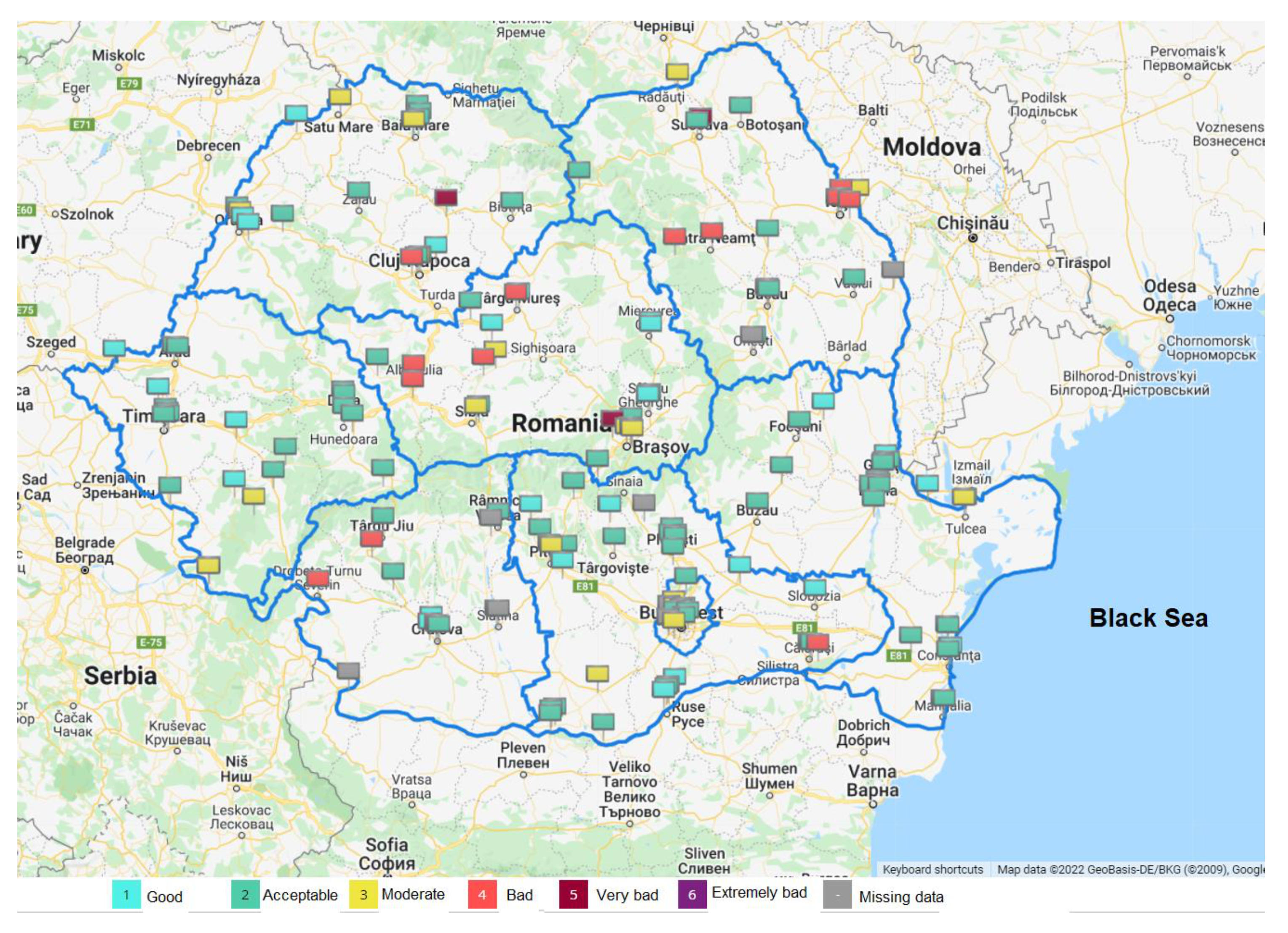
Figure 1. Map of the air quality in Romania (updated 22 March 8:20:00) (retrieved from https://www.calitateaer.ro/public/home-page/?__locale=ro (accessed on 10 March 2022).
Atmosphere 13 00558 g001
Figure 2. (a) Timișoara city (with the air monitoring stations, TM-1, TM-2, TM-4, and TM-5); (b) Map of Romania (http://www.destination360.com/europe/romania/map (accessed on 20 March 2022)).
Atmosphere 13 00558 g002
Figure 3. The pollutants series: NO, NO2, NOx, and O3.
Atmosphere 13 00558 g003
Figure 4. (a) Hourly air quality at the studied station during the period 1–21 March 2021. (b) Annual average concentration of NO2.
Atmosphere 13 00558 g004aAtmosphere 13 00558 g004b
Figure 5. Recursive partitioning of the dataset. (a) shows much fewer splits needed to isolate an anomalous data point (indicated by arrow) compared to (b) where the data point indicated by arrow is normal.
Atmosphere 13 00558 g005
Figure 6. The structure of a GRNN.
Atmosphere 13 00558 g006
Figure 7. The flowchart of the study.
Atmosphere 13 00558 g007
Figure 8. Histograms of the studied series: (a) NO, (b) NO2, (c) NOx, (d) O3.
Atmosphere 13 00558 g008
Figure 9. Charts of the autocorrelation functions (ACFs) for the data series. The blue lines represent the limits of the confidence intervals at a confidence level of 95%.
Atmosphere 13 00558 g009
Figure 10. Series charts and the anomalies computed by the isolation forest for (a) NO, (b) NO2, and (c) NOx series.
Atmosphere 13 00558 g010
Figure 11. (a) Series correlations; (b) Correlations of the anomalies detected by IF; (c) NOx and O3 series and their anomalies.
Atmosphere 13 00558 g011
Figure 12. Series charts and anomalies computed by the LOF for (a) NO, (b) NO2, (c) NOx, (d) O3.
Atmosphere 13 00558 g012
Figure 13. Series charts and the anomalies for (a) NO, (b) NO2, and (c) NOx, computed by GESD.
Atmosphere 13 00558 g013
Figure 14. ARIMA model for the NO2BC series. (a) NO2BC series and the estimated one. (b) The residual series in the ARIMA model. (c) The residual autocorrelation function. (d) The histogram of the residual series.
Atmosphere 13 00558 g014
Figure 15. GRNN model for the NO2BC series.
Atmosphere 13 00558 g015
Figure 16. Hybrid ARIMA—GRNN model for the raw series.
Atmosphere 13 00558 g016
Figure 17. (a) Residual correlogram and (b) histogram in the ARIMA(1,1,1) model for the series after the removal of aberrant values.
Atmosphere 13 00558 g017
Figure 18. The forecast based on the ARIMA(1,1,1) model—the blue line—and the confidence intervals at 95% and 90%—different nuances of grey.
Atmosphere 13 00558 g018
Figure 19. GRNN model for the NO2 series after the removal of anomalies.
Atmosphere 13 00558 g019
Figure 20. GRNN of the residual in the ARIMA(1,1,1) model for the series after the removal of anomalies.
Atmosphere 13 00558 g020
Figure 21. Actual vs. predicted values in the GRNN model of the residual from the ARIMA(1,1,1). after the removal of aberrant values.
Atmosphere 13 00558 g021
Figure 22. (a) The residual, (b) the histogram, and (c) the correlogram of the residual in the ARIMA(0,1,2) model for O3.
Atmosphere 13 00558 g022
Figure 23. The GRNN model for the O3 series.
Atmosphere 13 00558 g023
Table 1. Basic statistics of the pollutant series during the study period.
StatisticsNOxNONO2O3
min (µg/m3)0.001.600.0012.04
max (µg/m3)179.34150.1267.8691.28
mean (µg/m3)32.639.8715.6742.72
stdev (µg/m3)24.8116.2710.5318.71
cv0.761.640.670.44
skew3.005.281.780.33
kurt10.8237.004.64−0.66
Publisher’s Note: MDPI stays neutral with regard to jurisdictional claims in published maps and institutional affiliations.