Article

On the Detection of Snow Cover Changes over the Australian Snowy Mountains Using a Dynamic OBIA Approach

by
Aliakbar A. Rasouli
1,
Kevin K. W. Cheung
2,*,
Keyvan Mohammadzadeh Alajujeh
1 and
Fei Ji
3
1
Department of Climatology, University of Tabriz, Tabriz, Iran
2
E3-Complexity Consultant, Eastwood, NSW 2122, Australia
3
Climate and Atmospheric Science, NSW Department of Planning and Environment, Lidcombe, NSW 2141, Australia
*
Author to whom correspondence should be addressed.
Atmosphere 2022, 13(5), 826; https://doi.org/10.3390/atmos13050826
Submission received: 22 March 2022 / Revised: 29 April 2022 / Accepted: 17 May 2022 / Published: 18 May 2022
(This article belongs to the Section Climatology)

Abstract

:
This study detected the spatial changes in Snow Cover Area (SCA) over the Snowy Mountains in New South Wales, Australia. We applied a combination of Object-Based Image Analysis (OBIA) algorithms by segmentation, classification, and thresholding rules to extract the snow, water, vegetation, and non-vegetation land covers. For validation, the Maximum Snow Depths (MSDs) were collected at three local snow observation sites (namely Three Mile Dam, Spencer Creek, and Deep Creek) from 1984 to 2020. Multiple Landsat 5, 7, and 8 imageries extracted daily MSDs. The process was followed by applying an Estimation Scale Parameter (ESP) tool to build the local variance (LV) of object heterogeneity for each satellite scene. By matching the required segmentation parameters, the optimal separation step of the image objects was weighted for each of the image bands and the Digital Elevation Model (DEM). In the classification stage, a few land cover classes were initially assigned, and three different indices—Normalized Differential Vegetation Index (NDVI), Surface Water Index (SWI), and a Normalized Differential Snow Index (NDSI)—were created. These indices were used to adjust a few classification thresholds and ruleset functions. The resulting MSDs in all snow observation sites proves noticeable reduction trends during the study period. The SCA classified maps, with an overall accuracy of nearly 0.96, reveal non-significant trends, although with considerable fluctuations over the past 37 years. The variations concentrate in the north and south-east directions, to some extent with a similar pattern each year. Although the long-term changes in SCA are not significant, since 2006, the pattern of maximum values has decreased, with fewer fluctuations in wet and dry episodes. A preliminary analysis of climate drivers’ influences on MSD and SCA variability has also been performed. A dynamic indexing OBIA indicated that continuous processing of satellite images is an effective method of obtaining accurate spatial–temporal SCA information, which is critical for managing water resources and other geo-environmental investigations.

1. Introduction

Snow is a common global meteorological phenomenon, mostly on the Earth’s higher grounds. It is a valuable source of fresh water and is therefore regarded as an important component of the hydrological cycle [1,2]. Snow plays a significant role in influencing heat regimes and local, regional, and even global radiation balance [3,4]. As Darmody et al. [4] and Löffler [5] have demonstrated, snow strongly influences regional soil characteristics, plant composition, and community structure. At local levels, snow cover affects several soil parameters such as permeability, temperature, moisture, microbial activity, and carbon sequestration [6]. According to Lu et al. [7], snow’s distinct high surface reflectance and low thermal conductivity are believed to influence biological, chemical, and geological processes. In turn, several studies, such as Kargel et al. [8] and Chinn [9], noted that snow is a sensitive indicator of climate change.
In Australia, snow is mainly experienced from July to September in the Snowy Mountains [10]. The highest Australian mountain range is located in southern New South Wales and is part of the Great Dividing Range [11]. Whereas the prevalence of snow in the Snowy Mountains is not as high as in the northern hemisphere’s mid-latitudes and polar regions, the effects of annual snow are well documented [12]. Like other parts of the world, snow in this area causes different climatic conditions from the rest of Australia, landscape restrictions and land use, and ecological and agricultural differences. On the other side, the snow promotes soil water infiltration that re-invigorates grasslands and other natural vegetation, a particular supply of water and energy resources [13]. As such, mapping snow cover for this area is critical for sustainable utilization of catchments and planning for physical processes and tourism attractions [14].
Traditionally, field surveys have generated snow maps [15]. However, generating snow maps using survey techniques is often expensive, tedious, and time consuming [16]. Field surveys are therefore not ideal for the often quick-melting snow covers. Therefore, thematic snow cover types based on remotely sensed images have become popular over recent decades [17,18]. Remotely sensed datasets are particularly well suited for measuring snow cover due to their uniquely high incident radiation, contrasting with most natural and artificial surface types [19]. The suitability of remotely sensed datasets in snow cover mapping is further facilitated by repetitive temporal coverage, wide swath width, improved classification algorithms, and data acquisition from remote and inaccessible sites [20,21]. Up to now, many techniques have been exploited by scientists to map snow at various scales reliably. For details, one could be referred to Köning et al. [22], Foppa et al. [23], and Shreve et al. [24], who provided detailed overviews of some of the common remote sensing methods applied in snow mapping procedures.
Accurate remote snow cover mapping is valuable for planning, managing, and mitigating adverse biophysical and social processes [25]. One of the most successful satellite image-based snow mapping techniques is the Normalized Difference Snow Index (NDSI) proposed by Holroyd et al. [26] and Hall et al. [27]. This technique exploits the ratio between high snow reflectance and strong absorption in the electromagnetic spectrum’s visible and infrared sections [28]. Like most ratios, Salomonson and Appel [29] noted that one of the major advantages of NDSI is its resilience to atmospheric effects and influences caused by viewing geometry. In this regard, the remote sensing community’s utilization of NDSI has been widely adopted [30,31,32,33]. Whereas NDSI has been widely applied in mapping snow, the reliability of such maps is often compromised by its reflectance similarity with other land cover types such as clouds, water, shiny rock surfaces, and even vegetation covers [34]. According to Hall et al. [27], such features are characterized by low reflectance due to their high absorbance ability and low NDSI denominator. Under these circumstances, even a small increase in the infrared band may ultimately increase the NDSI and, therefore, cause misclassification of the alternative land cover type pixel as snow [35].
Consequently, there is still a need for techniques that we can use to improve the classification accuracy of snow cover maps by the processing of long-term satellite datasets. The Landsat imagery is one of the best candidates captured from Thematic Mapper (TM), Enhanced Thematic Mapper Plus (ETM+), and Operational Land Imager (OLI) sensors. These datasets have been extensively referenced in numerous studies in snow cover mapping over the past three decades [36,37].
OBIA classification involves segmenting an image into objects (groups of pixels) with geographical features such as shape and length, and topological entities such as adjacency (see Hellesen and Matikainen [38]). These attributes make a knowledge base for the sample objects, which can be called upon in the classification process, with a greater possibility for detecting snow cover in high-resolution imagery [39]. Originally, OBIA was one of several approaches developed to overcome the limitations of the pixel-based approaches to incorporate spectral, textural, and contextual information to identify thematic classes in an image. Such classification produces meaningful snow distribution maps by identifying individual pixels or groups of pixels with similar spectral responses to incoming radiation [40]. These pixels or groups represent different land cover classes, including SCA outlines. In practice, OBIA, as a sub-discipline of geo-information science, is devoted to partitioning remote sensing imagery into meaningful image objects and assessing their characteristics through spatial, spectral, and temporal scales [41]. Any object-based image analysis’ fundamental aim is to convert scene image objects into different sorts of practical land use-based information [42,43].
The present research has several objectives: (a) to detect the spatial changes in SCA over the Snowy Mountains by applying OBIA algorithms, (b) to demonstrate the precision of land cover classification related to snow index, and (c) to examine the long-term changes in the amount of snow depth and snow cover in the study area. To accomplish these objectives, a progressive set of dynamic OBIA methods was applied to process the Landsat imagery adapted to the Australian Snowy Mountains over a long period. To improve the outputs, we initially developed an ESP tool in the weighted segmentation process that subdivides any Landsat image into separated regions represented by basic unclassified image objects called ‘image object primitives’ [44]. Then, to extract better snow cover surfaces with high precision, NDSI, SWI, and NDVI were independently extracted and modified inside the eCognition 9.5 software [45]. Intending to highlight the water, vegetation, non-vegetation, and snow cover classes, we applied certain rule-based classification methods to classify these surfaces. Lastly, sets of dynamic thresholds were purposely accomplished in the accurate delineation of the SCA class from the others in the study area.

2. Study Area and Data

2.1. Study Area

The Snowy Mountains represent the highest Australian mountain range in southern New South Wales and are part of the larger mountain mass called the Australian Alps and the Great Dividing Range [46]. As the highest mountain in Australia, Mount Kosciuszko is 2228 m in altitude. The alpine climate is characterized by cool, crisp air; inside the region, temperatures average from minus 6 degrees Celsius in July and 21 degrees Celsius in January [47]. The Snowy Mountains comprise a few regions that experience four distinct seasons, being the only part of mainland Australia to be covered by glaciers during the most recent ice age, with some glacial lakes left by a paleo-climatic process [48]. Considering the importance of some geographic and environmental facts, Kosciuszko National Park was given international significance by being declared a World Biosphere Reserve by UNESCO [49,50]. Such a region is home to some of the country’s best nature-based activities and ski adventures, with beautiful peaks, great ski fields, and plenty of untamed Australian wildernesses to explore.
Figure 1 (upper) illustrates the geographic location of the Snowy Mountains in Australia and inside New South Wales and the Australian Capital Territory (ACT). A Landsat image footprint is set under the study area outline, and the position of the snow depth stations is shown by yellow numbers (1, 2, and 3) on the map. The outline of the study area roughly covers the region between 148.4° E, −35.4° S and 148.7° E, −36.95° S. This region has the longest snow/ice cover periods during the climate calendar each year [51,52]. In addition to being one of Australia’s best-known attractive touristic spots, the Snowy Mountains convert considerable hydroelectric power to offset the disastrous effects of droughts and as a sustainable development scheme. The topographic features of the study area, which is based on the Advanced Spaceborne Thermal Emission and Reflection Radiometer (ASTER) DEM data (with ~30 m resolution, vertical absolute (RMSE) error ~16 m (9.7 m) with 90% confidence) from NASA [53], are indicated in Figure 1 (lower). By simultaneous processing of DEM data and Landsat images, it is possible to determine altitude, slope, or aspect effects on the spatial distribution of snow cover. DEM data is also suitable for matching binary snow layers developed from Landsat scenes. Furthermore, we added a vector polygon layer in shapefile format to help mark the study area at the raster clipping process.
The Snowy Hydro is the largest hydroelectric scheme in Australia. It diverts the reliable waters of the south-flowing Snowy River westwards, beneath the Great Dividing Range, and provides electric power and additional water for the Murray and Murrumbidgee Rivers to be used for irrigation purposes [13].

2.2. Datasets Used

In the present study, datasets were collected to detect the longer-term SCA changes inside the study area. First, we collected the MSD data at three snow observation sites, namely Spencers Creek, Deep Creek, and Three Mile Dam, from 1984 to 2020. The Australian Snowy Hydro Groups undertake snow depth readings as required for operational purposes during the snow season [14]. Due to the high accuracy of the data observed at Spencers Creek station and the proximity of other snow depth recording stations, it was employed as a reference station. In the next step, Landsat satellite images, adapted for MSD dates, were taken from the NASA website [54].
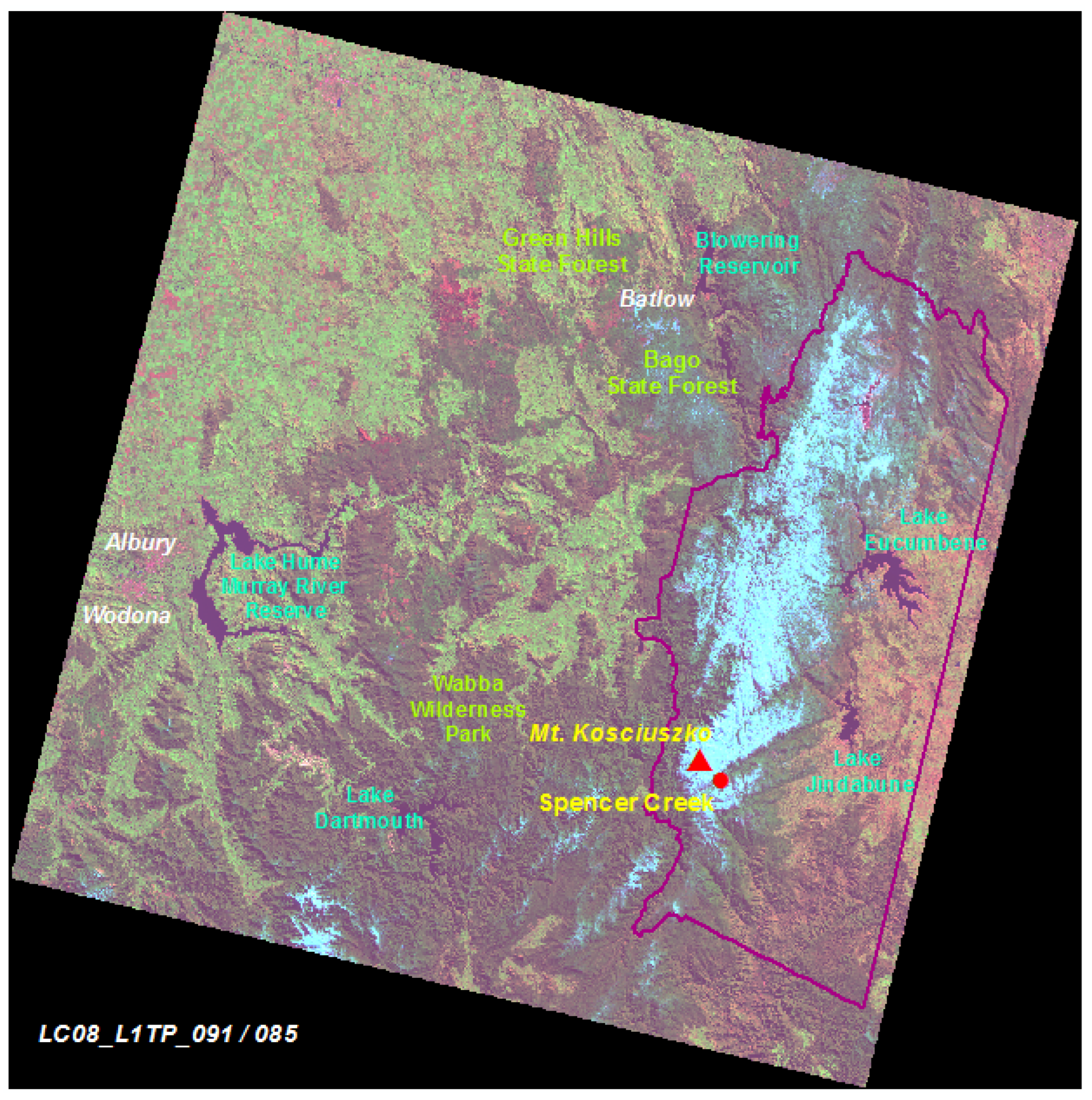
We should note that we took images for the same MSD dates’ maximum with a back–forth mismatch of 1–3 days. We processed multi-temporal Landsat series (5, 7, and 8) images, including Multispectral Scanner (MSS), Thematic Mapper (TM), Enhanced Thematic Mapper Plus (ETM+), and Operational Land Imager (OLI), to illustrate the spatial changes of SCA [55]. An example of a Landsat image is shown in Figure 2 for the cold season, with the maximum snow cover and associated neighbour geographic features.
The correlations between the variability of MSD, SCA, and the large-scale climate drivers in the Australian region are examined in this study. These climate drivers include the El Niño Southern Oscillation, the Indian Ocean Dipole, and the Southern Annular Mode (SAM). The indices to measure these climate models are the Southern Oscillation Index (SOI), the Dipole Mode Index (DMI), and the SAM index. The SOI and DMI indices are obtained from the Australian Bureau of Meteorology (BoM), while the SAM index is obtained from U.S. Climate Prediction Centre.

3. Methodology

In the current analysis, we applied several methods to the Landsat datasets. First, based on the adapted MSD data, the digital number (DN) values of each Landsat image were converted to the top of atmosphere (TOA) reflectance inside the ERDAS Imagine software [56]. The conversion of the raw pixel DN to the TOA reflectance constitutes pre-processing and only represents the brightness characteristics of ground objects in the image [57,58].
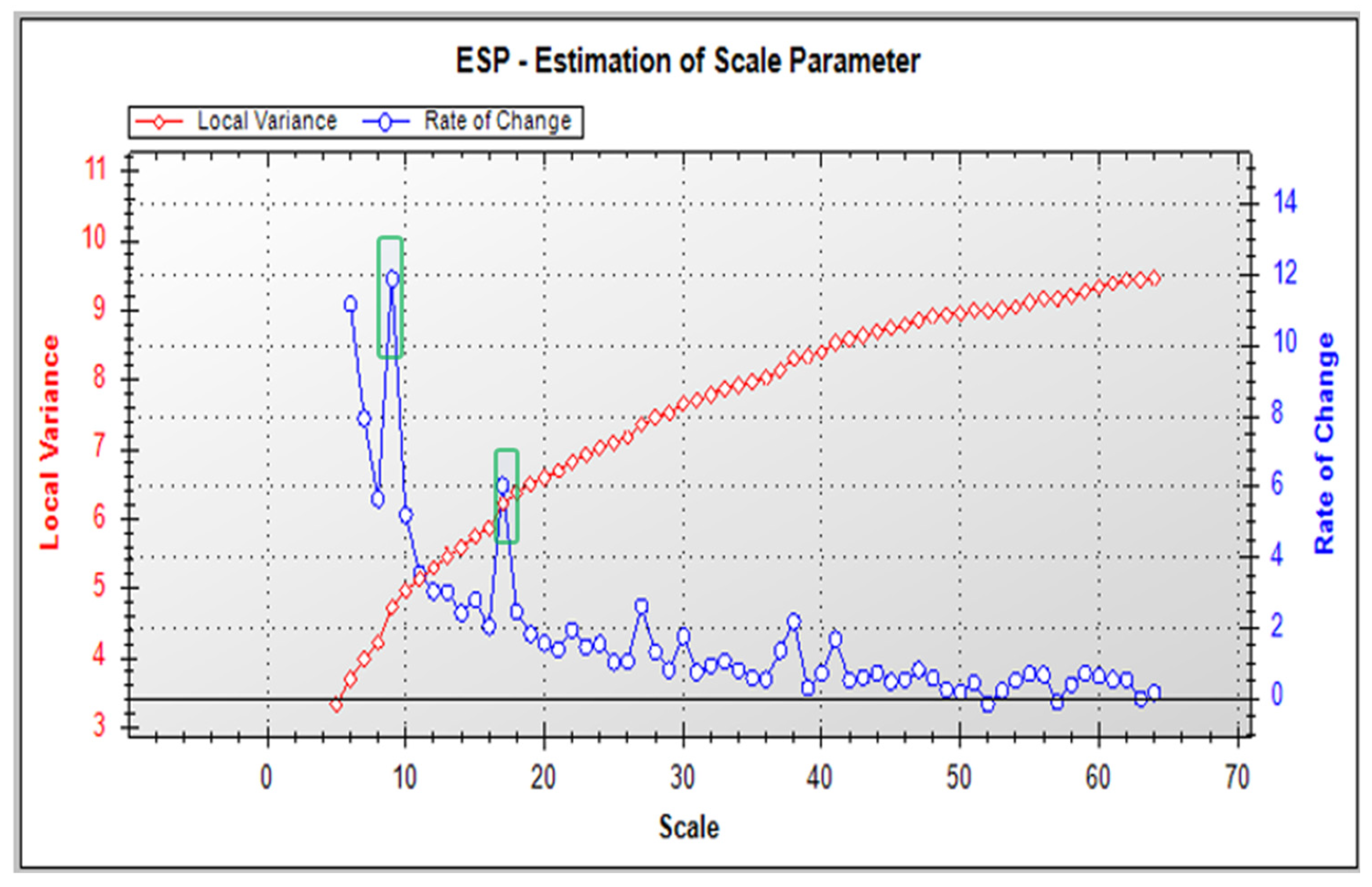
Then, we imported each corrected multispectral Landsat imagery to the eCognition software, creating mixed RGB layers. An Estimation of Scale Parameter (ESP) was applied to calculate well-justified scale parameters for each image scene [44]. When we modified segmentation settings based on the ESP, pixels of a Landsat image were grouped into image objects, depending on the image quality (e.g., bands available and spatial image resolution), before object-based classification could be performed. A subjective measure called the ‘scale parameter’ controlled the degree of heterogeneity within an image object. Moreover, we proposed the ESP tool, which builds on local variance (LV) of object heterogeneity within a scene. In practice, the ESP tool iteratively generates image objects at multiple scale levels and calculates the LV for each scale. Variation in heterogeneity is explored by evaluating LV plotted against the corresponding scale. The thresholds in rates of change of LV (ROC-LV) indicate the scale levels at which the image can be segmented most appropriately relative to the data properties at the scene level. The default value for the scale parameter is taken as about 10 in the segmentation stage of Landsat 5 and 7 images. For Landsat 8 images, this value is taken as 54. We suggested the shape and compactness indices as 0.4 and 0.5, respectively.
After that, a multi-resolution segmentation algorithm was applied to split each image into unclassified “object primitives” that form the basis for the image objects and the rest of the image analysis [59]. We set the segmentation and object primitives and eventual image objects’ resulting characteristics based on shape, size, colour, and pixel topology controlled through DEM parameters. The values of the parameters define the spectral and spatial characteristics of each image layer [60]. In SCA mapping, this process will require an understanding of image layer weights in the segmentation stage. Figure 3 indicates the ESP segmentation parameters, resulting in a “false-colour” image as snow shows up as light blue. The reddish indicates vegetation types, and the black colour is evidence of water bodies.
We created three basic snow, water, and vegetation classes in the classification step. Other land cover types, such as rock outcrops, bare lands, and background classes, were additionally assigned inside the Class Hierarchy [61]. Along with implementing a dynamic rule-based classification, we applied a set of equations in a stepwise manner to create the basic indices (Table 1).
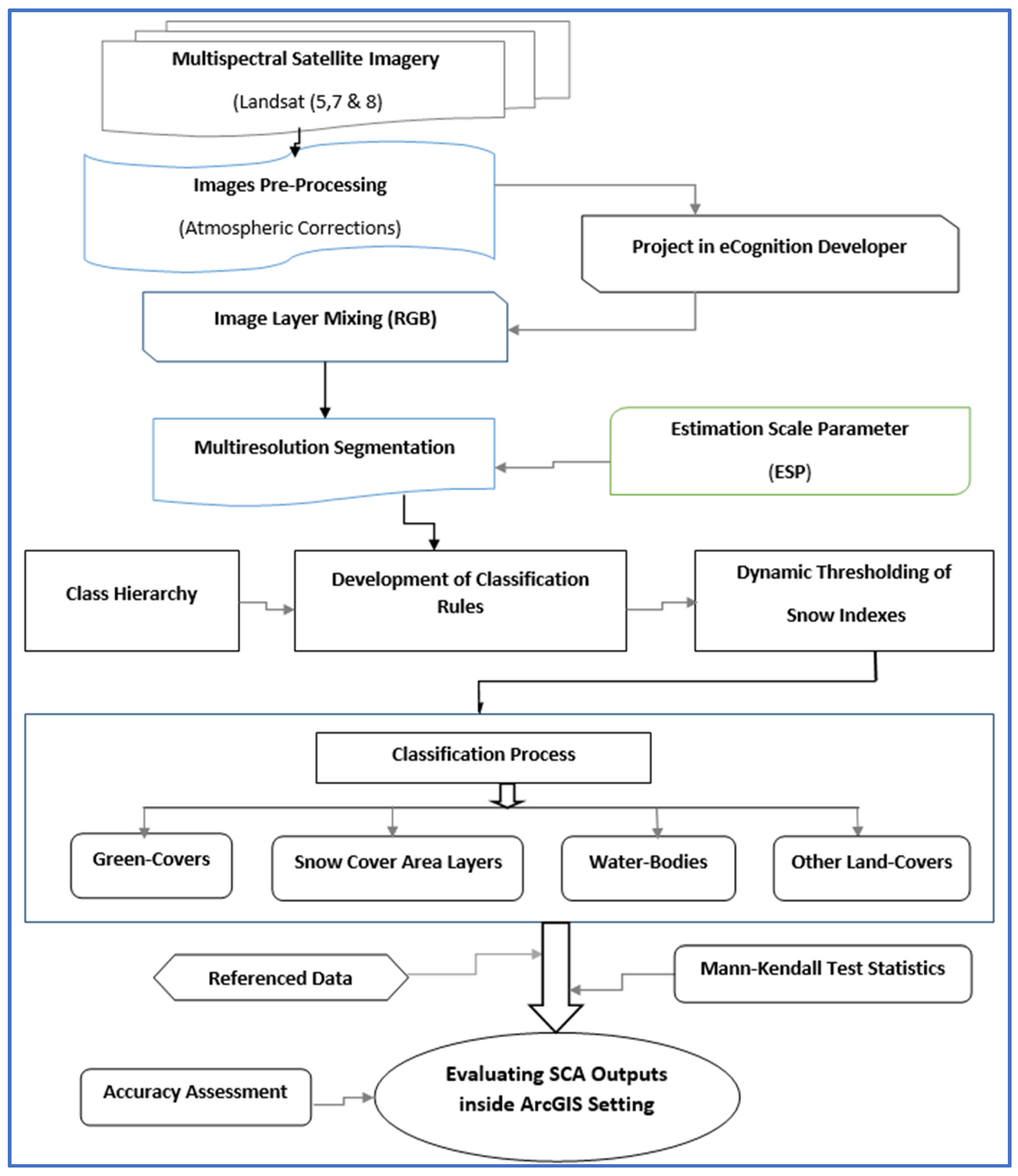
In the dynamic thresholding stage, each index is regarded as an indicator or measure of a specified land cover, typically referring to a spectral measure of the change in the Landsat image band reflections [62]. Inside the eCognition Developer, an Index layer calculation algorithm inserts a new image layer by calculating a spectral index differentiating between NDVI, NDWI, and NDSI classes [63,64]. Before the final analysis of SCA maps, a sampling procedure was applied for each class, and the software created a TTA mask to assess the classification accuracy [17]. We exported all recognized snow classes to the ArcGIS setting for later analysis at the final stage. Figure A1 in Appendix A provides an overview of the current workflow process for extracting SCA based on the OBIA method.

4. Results

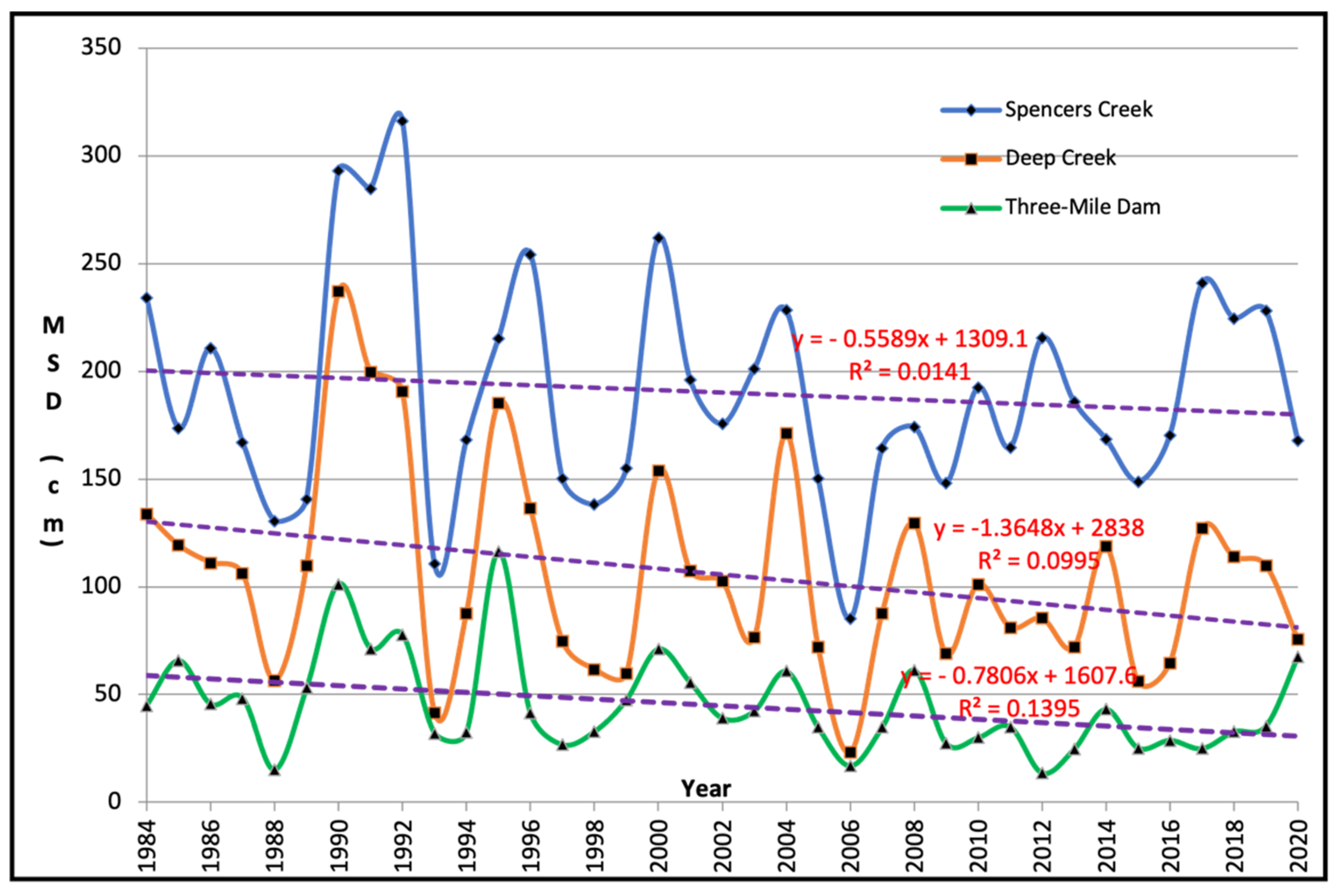
Traditionally, MSDs are observed by the Snowy Hydro Company during the cold months and are updated at the three snow depth sites. Analysis of MSD data from 1984 to 2020 at Spencers Creek, Deep Creek, and Three Mile Dam gave negative trends of −1.36, −0.54, and −0.78 cm per year, respectively (Figure 4). These trends represent percentage changes with explained variances (R2) of 0.014, 0.099, and 0.139. None of these trends are statistically significant at 95% confidence. While the highest MSD values were recorded at Spencers Creek, the lowest trend is also noticeable at this site, with the lowest R2 value of 0.014. Data at the three stations are available from as early as 1954. The long-term variability of the measured MSDs at Spencers Creek is shown in Figure A2 and Figure A3 of Appendix B.
The monthly distribution of MSDs and linear correlation values between recording stations is presented in Table 2. August is the month with the highest frequency of MSDs, with nearly 53% of observations. The Spencers Creek site has the highest snow depth values. Nevertheless, the observations at the three sites are highly correlated (with pairwise correlation coefficients of 0.86, 0.55, and 0.80, respectively).
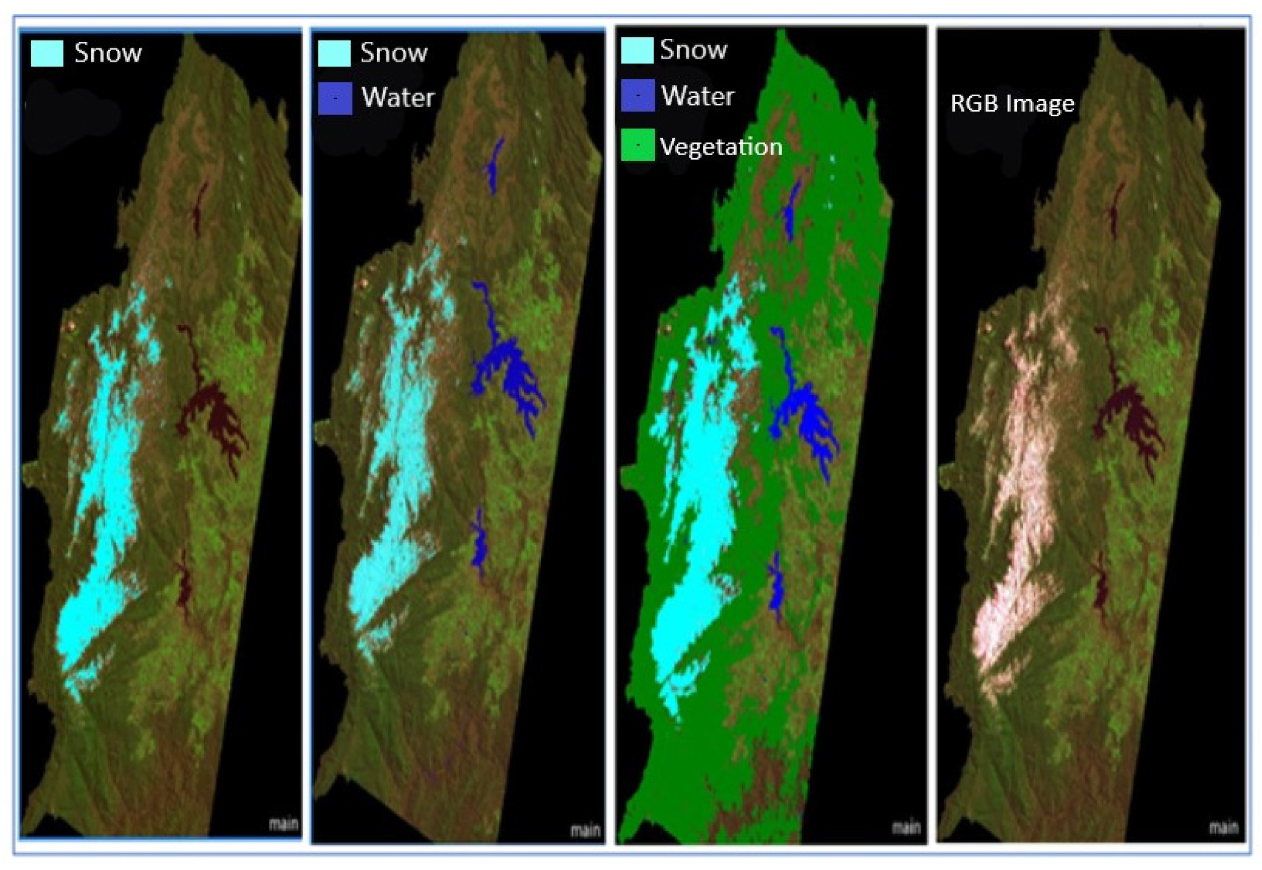
The relevant indices of NDSI, SWI, and NDVI are shown in Figure 5, which illustrates the stepwise identification of the snow, water bodies, and vegetation compared to an RGB image.
An accuracy assessment tool was run within the eCognition Developer when the rule-based supervised classification was accomplished. The goal of this stage was to generate a typical error matrix that computes the user’s and producer’s accuracies, the Kappa Index of Agreement (KIA), and other statistics related to the accuracy of the classification procedures [65]. You can find the details in such accuracy assessment and the definitions of these measures in Appendix C. Overall Accuracy (OA) tells us our correctly mapped proportions out of all reference sites. The overall accuracy is usually expressed as a percentage, with 100% accuracy being a perfect classification, where all reference sites are classified.
The Kappa Statistic or Cohen’s Kappa is a statistical measure of inter-rater reliability for categorical variables [66]. In this study, Kappa is used when two raters apply a criterion based on a tool to assess whether or not some condition occurs. The results of accuracy assessments are shown in Table 3.
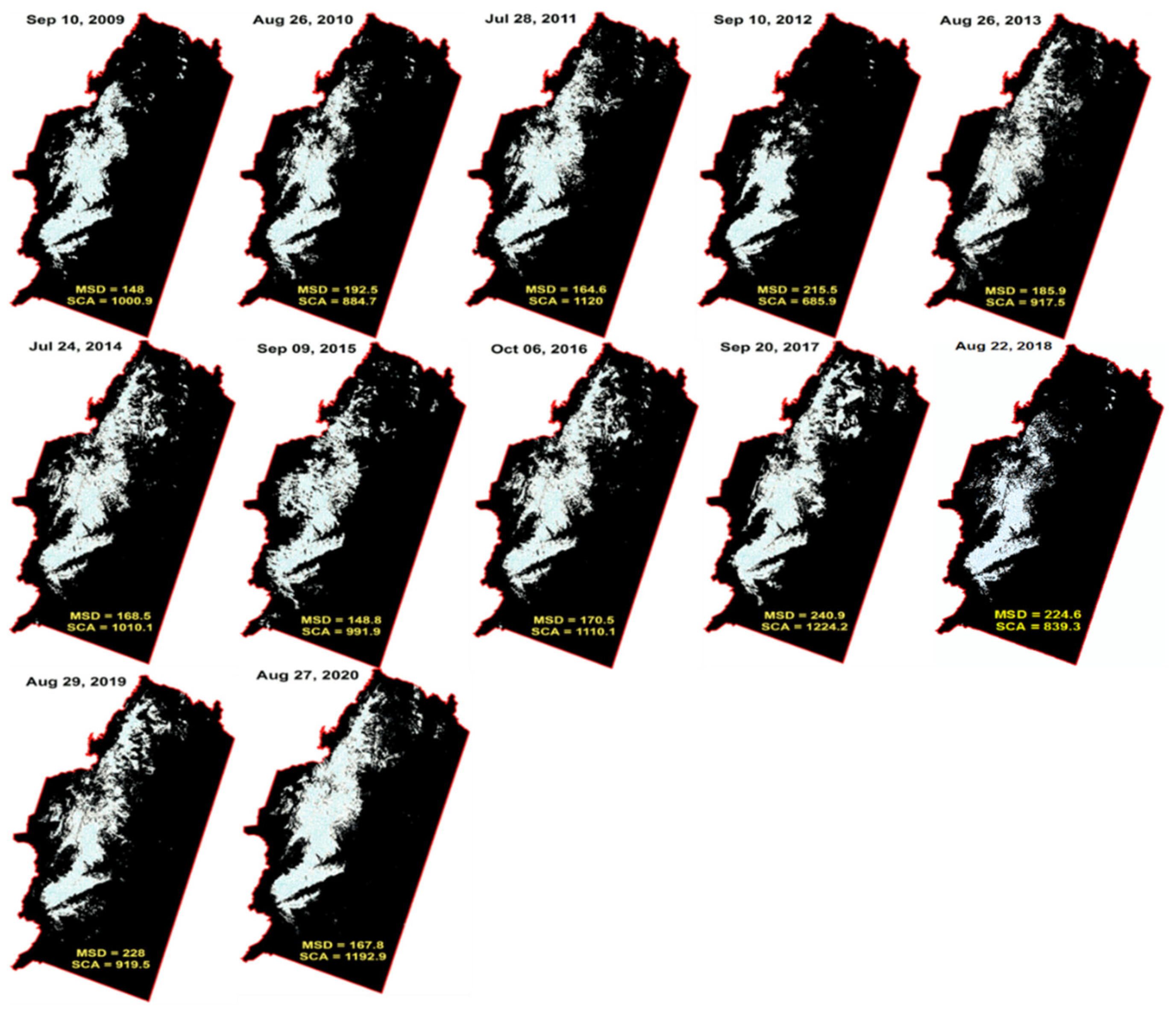
We transferred the final classified shapefiles to the ArcGIS setting, and only the snow class was separated and illustrated. The SCA temporal–spatial variations inside the selected Snowy Mountains area are indicated in Figure 6.
Regarding the changes in the SCA amount, we should highlight some obvious facts. First, despite changes in the area of SCA, its shape and form remain almost constant. Second, there is always constant snow cover over the high-altitude ranges (mostly above 1500 m), which can be seen in all years. Areas with constant SCA can be seen in the Snowy Mountains’ highest spots and valleys, where the topographic surfaces play very important roles in the long-term maintenance of snow reserves and water supply. Both are vital for tourist entertainment and the supply of agricultural and urban water resources [67].
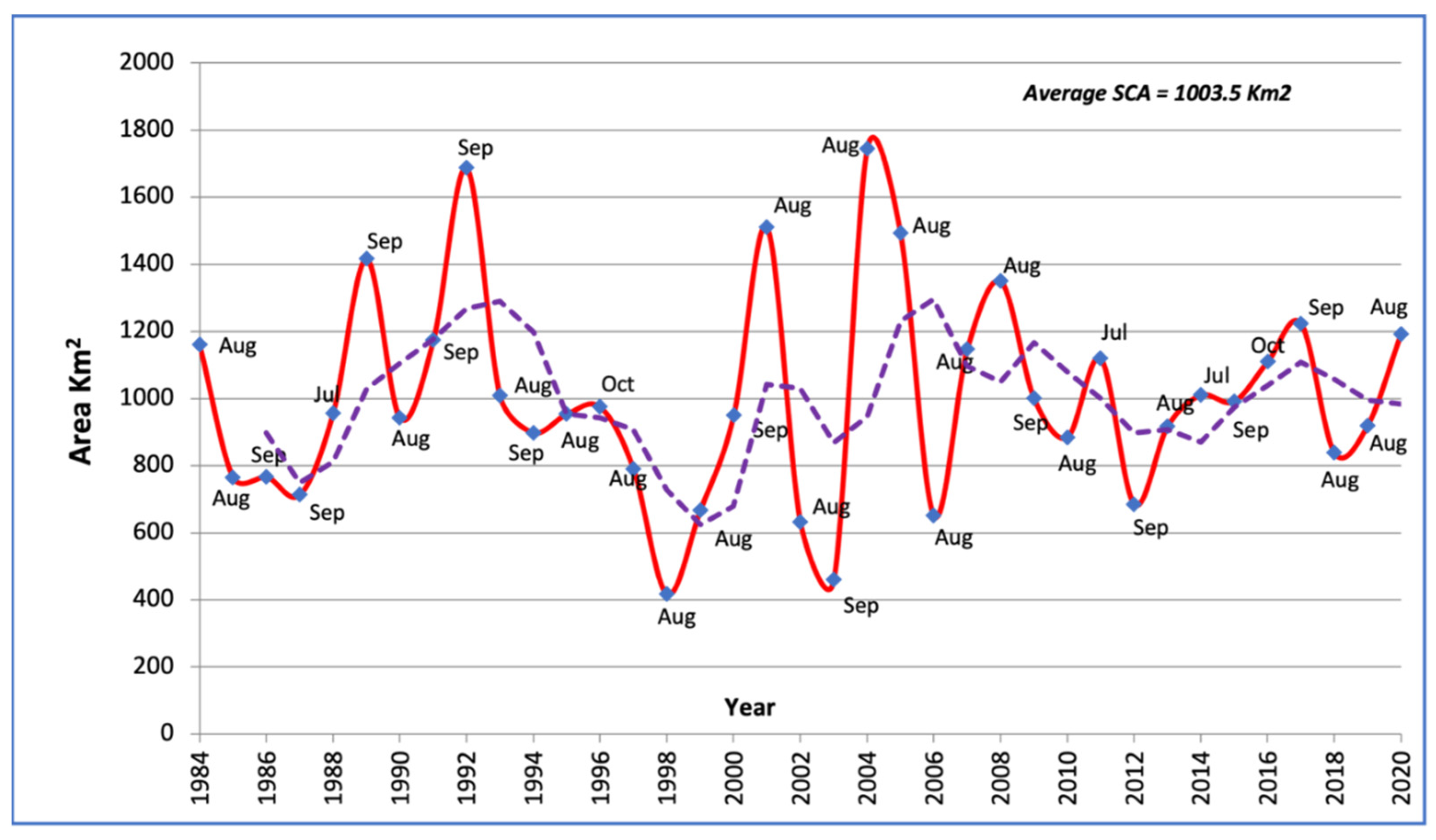
A visual review of sampled snow maps in Figure 6 and relevant statistics explain that significant fluctuations have occurred over the Snowy Mountains over the past 37 years (Figure 7). SCA fluctuates greatly over time, with a maximum frequency in August and September. Although no significant decreasing changes are seen in the SCA, it still appears that from 2006 onwards, there is a significant drop in the absolute values, as this type of change is also evident in the 3-year moving average trend.
Since SCA is the major parameter we extracted from the Landsat images, it is interesting to examine its correlation with the MSD measured at the three sites. There is a moderate correlation that can be identified. The correlation coefficient between SCA and MSD at Spencers Creek is 0.28 (significant with 90% confidence), that between SCA and Deep Creek is 0.38 (significant with 95% confidence), while that between SCA and Three Mile Dam is 0.29 (significant with 90% confidence). These results indicate that the extent of snow cover does vary with the snow depth.
Moreover, as a preliminary analysis, the correlations between the MSD and SCA time series with the major modes of climate variability in the Australian region (namely, ENSO, IOD, and SAM) have been examined via the indices indicating the phases of these climate modes (i.e., SOI, DMI, and the SAM index). The anomalies of the MSD/SCA and the climate indices were prepared before the correlation analysis [10]. Since the MSD/SCA was reported for a month each year, we selected the corresponding month in the climate indices to form the interannual time series. Only marginal correlations were identified using the entire record of the MSD data measured at Spencers Creek from 1954 to 2020. The correlation coefficient between MSD (SC) and SOI is 0.23, significant at 90% confidence; that between MSD (SC) and DMI is −0.19, again, significant at 90% confidence. However, none of the correlations were statistically significant, including the SAM index, when we analysed only the short period 1984–2020. These results are mostly consistent with Pepler et al. [68], who performed correlation analysis based on seasonal averages. They did identify a significant correlation with SAM, which may be due to the longer period of the SAM index they applied. Pepler et al. found that the responses of MSD to the climate drivers are not the same before and after 1984. This preliminary analysis indicates that natural climate variability, other than climate change, contributes to the variability of MSD and SCA. However, physical process analysis, such as through climate downscaling, must be further investigated to understand such impacts.

5. Discussion

Snow cover has to be regarded as one of the most sensitive weather and key climatic elements that affect other natural resources [69]. Over the years, several interrelated factors have influenced gradual technological progress in mapping snow-cover and applying remote sensing data. Advancements in satellite sensor and image-processing technologies have caused demands for accurate and frequent monitoring of SCA. Due to rapid industrialization, urbanization, and changing climate, snow cover changes are occurring faster [70]. Therefore, regular and precise mapping of snow-covered regions is important for several reasons, such as continuous snow cover monitoring from high-resolution satellites, accurate snow hydrology management, and possibilities for drought assessment. In addition, snow cover detection is an important driver of many climatic, hydrological, and ecological processes and is a required input to many models aiming to study and predict them [71]. For example, a recent study showed that the simulated snow depth trends in the Sixth Coupled Models Intercomparison Project (CMIP6) conflict with observations [72]. Thus, robust monitoring of SCA and MSD is critical.
SCA is also one of the essential climate variables specified by the Global Climate Observing System to be observed by remote sensing in support of the United Nations Framework Convention on Climate Change and the Intergovernmental Panel on Climate Change [73]. The present study showed that, firstly, the amounts of MSD in the study area are tangible but decreasing. The result of this research is somewhat in line with the findings of [74], which depicted the impact of climate change on snow conditions in mainland Australia. Variability in SCA is highly regional, similarly to the trends identified for the European Alps [75]. Thus, the trend and variability identified in this study have provided a valuable baseline to study the climate factors behind the SCA changes.
Multiple methodologies have been designed to observe snow cover using optical and SAR satellites applying different analytical methods [76,77]. This study aimed to process low-cloud optical Landsat images to create SCA layers based on dynamic OBIA rule-based and thresholding methods [78]. Over recent decades, the processing of digital satellite digital images has been one of the most important methods for extracting snow cover information, which is performed by two general methods of pixel-based processing and object-based processing [79,80]. Many researchers used to process image pixels in the past and have only applied the NDSI algorithm to estimate snow cover levels. Therefore, pixels recognized as snow may contain snow cover and other land uses, particularly clouds, which reduces the precision of snow cover extraction and makes extracting all snow covers complicated. Due to the low spatial resolution of satellite imageries, separation and extraction of snow cover from the cloud cover is done with very low accuracy [81].
On the other side, the OBIA method is based on the segmentation of numerical values of images. The latter uses numerical values, content, texture, and background information in the image classification process [82]. Due to the higher accuracy of object-oriented classification compared to pixel-based classification, over recent years, many researchers have tried to classify and estimate SCA based on the shape, texture, and grey tone of changes in image objects that resolve the pixel blend problems. Despite implementing the above methods, it is still observed that the snow zones are not completely separated in some cases.
To increase the accuracy of SCA maps in the current research, we tried to improve the OBIA methods with a few changes adopted to the Landsat satellites. We implemented an ESP tool to estimate accurate parameters that separated optimal image objects in the segmentation stage. We gave higher weights to a few layers (bands) of Landsat imagery. We considered the ASTER DEM rule to optimize segmentation procedures that made it possible to increase the level of separated objects’ information. Certainly, to calculate the exact inherent relationships between topographic parameters (such as altitude, slope, and aspect) and SCA variations, we will need higher-spatial resolution data such as AlOS-Palsar (with 12.5 m2) and higher-spatial-scale satellite images (Sentinel 2A, with 10 m2). Applying complementary rule-based functions such as threshold classifications can increase the accuracy of the final NDSI maps [83]. In future research, adapted deep learning approaches will help assign each object to specific land use classes by offering accurate information on the snow cover changes [66].
The present study has only extracted from the Landsat images. Meanwhile, other optical sensors, such as Sentinel-2, may be considered to improve the SCA maps’ accuracy. Sentinel-2 has a lower temporal resolution than the Landsat OLI, and we may combine their high-spatial resolution bands to achieve better results in future studies [84,85]. It is also worthwhile to test the sensitivity of ALOS-Palsar DEM data to reconstruct fine SCA datasets and associated products such as snow depth and snow water equivalence (SWE) [86,87,88,89].
In a global context, changes in snow cover and related phenology (duration, onset, and melt) have a critical role in the mountain environment and water availability in downstream areas [90]. Most researchers have found that the temperature increase in mountains may double the global average, intensifying with elevation [91]. Beniston et al. [92] reviewed the status of the European mountain cryosphere, indicating that the existing negative trends for snow depth and snow water equivalent are related to snow cover changes. They found that the Alps present negative trends below 2000 m, whereas no clear trend is found above this altitude. On the other side, in the Swiss Alps, Klein et al. [93] found a decline at both lower and higher elevations. Some contrasting trends were identified, as well in the Fennoscandian mountain areas. Other European Mountain regions in Spain, Romania, Croatia, and Bulgaria show a snowpack reduction. The main reason for the observed changes is a decrease in solid precipitation and more intense melt related to increasing air temperature in winter and spring. Notarnicola [94] provided a consistent picture of snow cover changes in global mountain areas to understand the evolution over the last 18 years. The study indicated that significant snow cover duration changes are related in 58% of the areas to both delayed snow onset and earlier melt. Moreover, the rate of earlier snowmelt is greater than the rate of later snow onset in the analysed period. Generally speaking, most investigations believe such changes have multiple impacts on water resources, ecosystem services, tourism, and energy production. All these studies indicated that SCA changes have a profound and cascading impact on the mountain environment. Such changes could seriously affect the surrounding’s physical geographical features and several socio-economic sectors.

6. Conclusions

This study demonstrated that SCA over the Snowy Mountains in New South Wales, Australia can be mapped based on the processing of Landsat imagery (from Landsat 5, 7, and 8) by applying a set of dynamic OBIA techniques, including segmentation, classification, and thresholding rules to extract the snow, water, vegetation, and non-vegetation land covers. This method is a trustworthy alternative to snow measurement stations, which are limited in many geographic locations. Three different indices (NDVI, SWI, and the NDSI) were created. Validation for these indices is the MSD collected at three local snow observation sites (namely Three Mile Dam, Spencer Creek, and Deep Creek) from 1984 to 2020. In fact, many techniques have been developed to extract snow information from satellite images other than the NSDI applied in this study. We have discussed some of these techniques in Appendix D, in particular, the Normalized Differential Snow Thermal Index (NDSTI) in Appendix E.
Although the resulting MSD data from all snow observation sites show noticeable reduction trends during the study period, the SCA-classified maps reveal non-significant trends and display considerable fluctuations over the past 37 years. The variations are concentrated in the north and south-east directions, to some extent with a similar pattern each year. Since 2006, the pattern of maximum values has decreased, with fewer fluctuations in wet and dry episodes. A preliminary analysis of climate drivers’ influences on MSD and SCA variability has also been performed. The MSD at Spencers Creek is significantly correlated to ENSO and IOD, while not with SAM. The correlations of these climate drivers with SCA are not statistically significant.
A dynamic indexing OBIA indicated that continuous processing of satellite images is an effective method of obtaining accurate spatial–temporal SCA information, which is critical for managing water resources and other geo-environmental investigations. Although the NDSI and supervised classification produced comparable results, a dynamic OBIA approach offers a higher classification accuracy. Moreover, a hybrid deep learning and object-oriented method could be applied to detect SCA, with its details compared with high-resolution topographic parameters. More importantly, Markov chain analysis procedures may provide comparable maps of the SCA changes to gain realistic future models for decision makers. Two major factors can be highlighted as recommendations for water resource management running the Snowy Hydro industry. First, climate change could alter the area of snow cover area, snow depth, and snow water equivalent factors in the near future around the Snowy Mountains. Secondly, SCA changes could affect water recourses, vegetation patterns, and derange systems, especially along the Murray River basin. Accordingly, timely and accurate information on snow components, extracted by a real-time remote sensing approach, could be incorporated into existing management tools, principally by the Australian government authorities and associated research organizations.

Author Contributions

Conceptualization, A.A.R., K.K.W.C. and F.J.; methodology, A.A.R.; software, K.M.A.; validation, A.A.R., K.K.W.C. and K.M.A.; formal analysis, A.A.R.; investigation, K.M.A.; resources, A.A.R.; data curation, K.M.A.; writing—original draft preparation, A.A.R.; writing—review and editing, K.K.W.C. and F.J.; visualization, K.M.A.; supervision, A.A.R. and K.K.W.C.; project administration, A.A.R. All authors have read and agreed to the published version of the manuscript.

Funding

This research received no external funding.

Institutional Review Board Statement

Not applicable.

Informed Consent Statement

Not applicable.

Data Availability Statement

The data applied in this study are available from the authors.

Acknowledgments

We would like to thank many people who made the research achievable. First, we appreciate the Faculty of Science and Engineering, Department of Earth and Environmental Sciences academic and professional staff at Macquarie University for providing many research facilities for Professor Rasouli during his academic fellow collaboration. Special thanks to the Australian Snowy Hydro for providing snow depth data and their people’s environmentally secure visions. We downloaded Landsat ETM+ scenes from http://glovis.usgs.gov/ (accessed on 16 May 2022) and the ASTER global digital elevation models (DEM) from the NASA web interface Reverb (http://reverb.echo.nasa.gov/reverb, accessed on 16 May 2022). The authors gratefully acknowledge these facilities and freely available valuable datasets. The SOI and DMI indices were downloaded from the BoM climate website (http://www.bom.gov.au/climate/influences/graphs/, accessed on 16 May 2022). The SAM index (also named the Antarctic Oscillation) was downloaded from the US Climate Prediction Center website (https://www.cpc.ncep.noaa.gov/products/precip/CWlink/daily_ao_index/aao/aao.shtml, accessed on 16 May 2022).

Conflicts of Interest

The authors declare no conflict of interest.

Appendix A

The figure in this appendix provides an overview of the process in the research workflow for extracting SCA data based on the OBIA method.
Figure A1. The workflow of the extraction of SCA maps.
Atmosphere 13 00826 g0a1

Appendix B

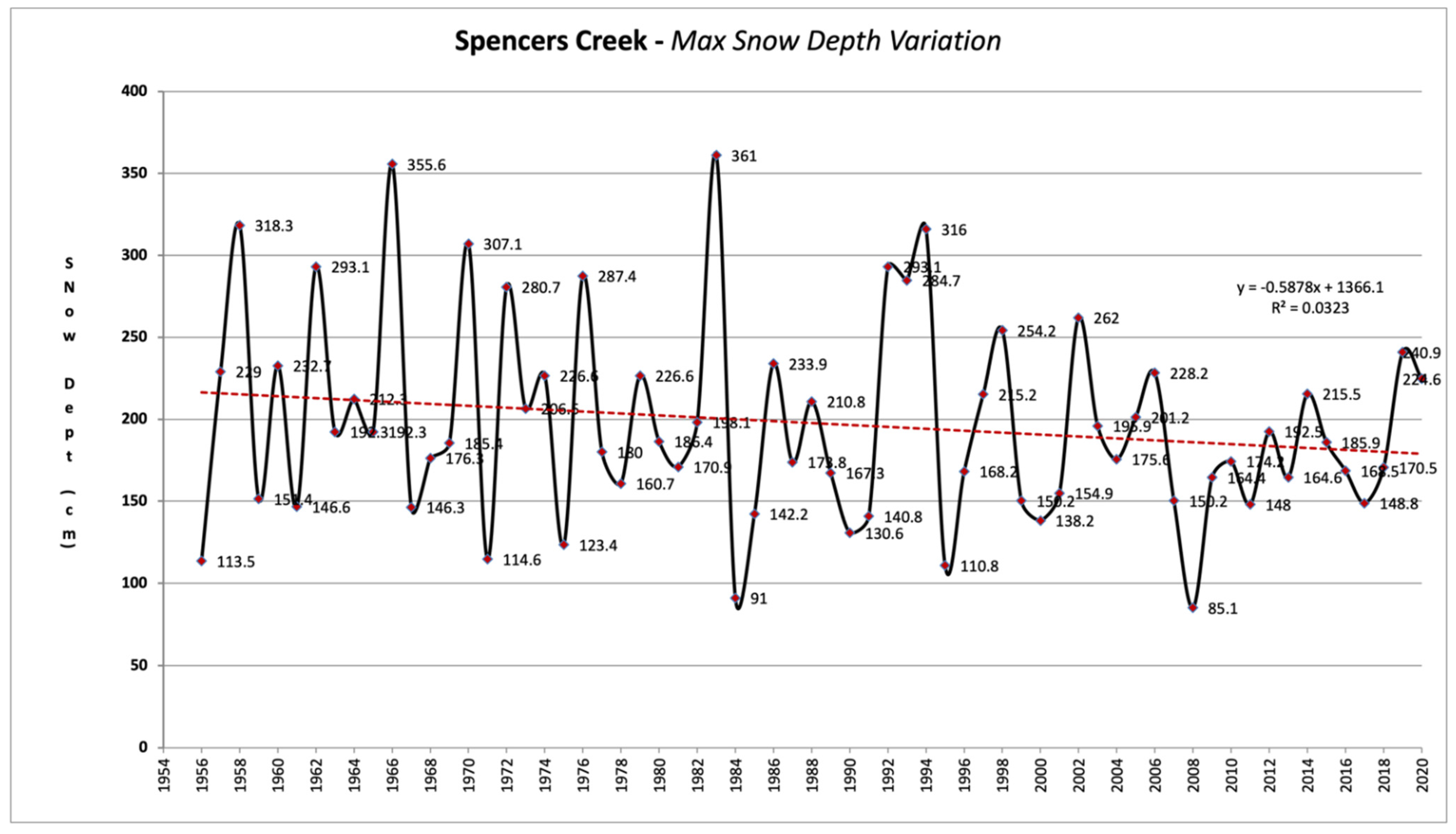
Among the three snow depth measurement stations in the Snowy Mountains, the Spencers Creek station usually measures the largest MSD values. The data at the three stations are available starting from 1954. Thus, the MSD measured at Spencers Creek from 1954 to 2020 is shown in Figure A2 to illustrate its long-term variability and trend.
It can be seen that, similar to the shorter time series shown in Figure 5, the interannual variability in the entire data period is also large. Nevertheless, there is still a long-term decreasing trend over the decades. The seasonal Mann–Kendall test was conducted after we removed autocorrelation from the time series to estimate the trend’s robustness. Figure A3 shows the Mann–Kendall statistic for each year (i.e., for a time series from 1954 up to a particular year). We can see that from about 1984, the statistics are almost all negative, indicating a negative trend. Since this normalized statistic follows the normal distribution, the decreasing trend is significant at the 90% confidence level after 2008.
Figure A2. Interannual time series of the observed MSD at the Spencers Creek observation site (solid line). The linear regression line with explained variance is shown.
Atmosphere 13 00826 g0a2
Figure A3. Value of the Mann–Kandall statistic for a time series from 1954 up to a particular year (blue dot). The red dashed line is a third-order polynomial fit (the equation) to the data.
Atmosphere 13 00826 g0a3

Appendix C

Inside the eCognition Developer, when the classification is complete, it is common to examine the accuracy of the results [95]. This function provides users with the ‘Accuracy Assessment’ tool to produce statistical outputs to check the quality of the classification results. The classification error matrix typically contains tabulated results of accuracy evaluation for a thematic classification, such as a land use and land cover maps [96,97]. Diagonal elements of the matrix represent counts which are correct, and the usual designation of classification accuracy is total percent correct. Non-diagonal elements of the matrix are usually neglected. A coefficient of agreement is determined for the interpreted map as a whole and individually for each interpreted category. These coefficients utilize all cell values in the matrix. A conditional coefficient of agreement for individual categories is compared to other expressions of category accuracy [66].
We used the Accuracy Assessment Tool to generate a Confusion (Error) Matrix based on the validation image samples in the current study. By calculating the error matrix based on samples, it is possible to calculate the accuracy statistics for all classification classes selected. In Table 2, the upper parts indicate Error Matrix statistics. Usually, a Confusion Matrix is a table that is often used to describe the performance of a classification model (or “classifier”) on a set of test data for which the true values are known. The lower part represents the accuracy indices with the following definitions:
  • Producer Accuracy is the map accuracy from the point of view of the mapmaker (the producer). It often refers to the real features on the ground correctly shown on the classified map or the probability that a certain land cover of an area is classified as such. The producer’s accuracy indicates the proportion of the reference data classified correctly for a given class.
  • User Accuracy refers to how a classified map is real on the ground. The User Accuracy is the accuracy from the point of view of a map user, not the map maker. The User Accuracy essentially tells us how often the class on the map will be present on the ground.
  • The “Hellden” Accuracy indicates the mean accuracy (developed by [98]). This index denotes the probability that a randomly chosen point of a specific class on the map corresponds to the same class in the same position in the field, and that a randomly chosen point in the field of the same class corresponds to the same class in the same position on the map.
  • Another alternative index is the “Short” measure [98]. It can be interpreted as the ratio of the estimated and true classes’ intersection to their union in terms of set cardinality for a given class. It ranges from ‘no overlap’ to ‘complete overlap’.
  • Kappa’s Coefficient of Agreement is a measure of accuracy for thematic classification, and the coefficient of conditional Kappa is an accuracy measure for the individual category [99]. A family of such coefficients is correct for chance agreement, but the Kappa coefficient is one of few defensible intraclass correlation coefficients. These coefficients use the classification error matrix information resulting from commission errors and omission.

Appendix D

Scientists have exploited several techniques to historically map snow at various scales over recent decades [100]. They have provided a detailed overview of some common remote sensing datasets and methods used in snow mapping [101,102]. One of the most successful image-based snow mapping techniques is the NDSI proposed by Hall et al. [103]. As used in the current study, this technique exploits the ratio between snow’s high reflectance and strong absorption in the electromagnetic spectrum’s visible and short-wave infrared sections, respectively.
Other objective methods of monitoring snow-covered areas by optical remote sensing were also evaluated using synchronous observations conducted with the passage of the Landsat satellites over recent years. For example, a newly proposed snow index called S3 uses visible, near-infrared, and shortwave-infrared reflectance and is more useful than NDSI because it automatically distinguishes snow-covered areas from mixes of snow and vegetation [104]. They assessed the accuracy of S3 over NDSI, specifically in the areas where snow cover and forested areas overlapped each other.
Another index is NDSII-1, specially designed by Xiao et al. [105] for the VGT (Vegetation) sensor of the SPOT4 satellite, which was launched in 1998 to map snow and ice cover. The VGT sensor has four spectral bands (blue, red, near-infrared, and mid-infrared), which are equivalent to the Landsat TM bands. The NDSTI-1-based VGT approach is a simple and automatic way of monitoring and mapping snow and ice cover areas from landscapes to global scales. The concept behind the development of the NDSII-1 index is using the different aspects of snow reflectance in the red and SWIR bands of the VGT sensor. Landsat TM has the same spectral bands as VGT, so researchers have applied the NDSII-1 using Landsat TM to different world regions and compared it to the NDSI, where they found that NDSII-1 produced the same results as NDSI [103].
The Snow Cover Ratio (SCR) was also defined as the ratio of the number of pixels in snow-covered areas to the total number of pixels in an image [106]. The threshold value for the three indices used to identify snow-covered areas was 50% of SCR, which converged to nearly the same value regardless of the images analysed. Using this index, under clear conditions, visible (red) reflectance can identify snow-covered areas accurately if no vegetation is present.
Sibandze et al. [107] proposed a new technique that combines the Landsat imagery principal components generated using PCA with commonly used NDSI, referred to as Normalised Difference Principal Component Snow Index (NDPCSI). This technique was supposed to improve snow mapping accuracy. This study demonstrated that snow cover could be mapped using Landsat 8 imagery using NDSI and NDPCSI techniques. Although the NDSI and NDPCSI produced comparable results, the NDPCSI produced higher classification accuracy.
The Normalized Difference Snow Thermal Index (NDSTI) was proposed by Haq et al. [108] and has been found to identify snow and ice and separate snow/ice from surrounding features. The NDSTI is defined as the difference of reflectance observed in a visible band (blue) and the Thermal infrared (TIR) band divided by the sum of the two reflectances. The index uses the spectral characteristics of snow/ice, a high reflectance in the visible region, and strong absorption in the TIR region. It does not depend on reflectance in a single band. The resampling of the TIR band was performed concerning the visible band. The TIR wavelength range of 10.40–12.50 µm (Landsat Band 6) and 8.125–8.175 µm (ASTER Band 10) is typical in many current space-borne multispectral sensors.
Meanwhile, Salomonson and Appel [28] noted that one of the major advantages of NDSI is its resilience to atmospheric effects and influences caused by viewing geometry. In this regard, use of NDSI has been widely adopted by the remote sensing community (see [4,109,110], among others).

Appendix E

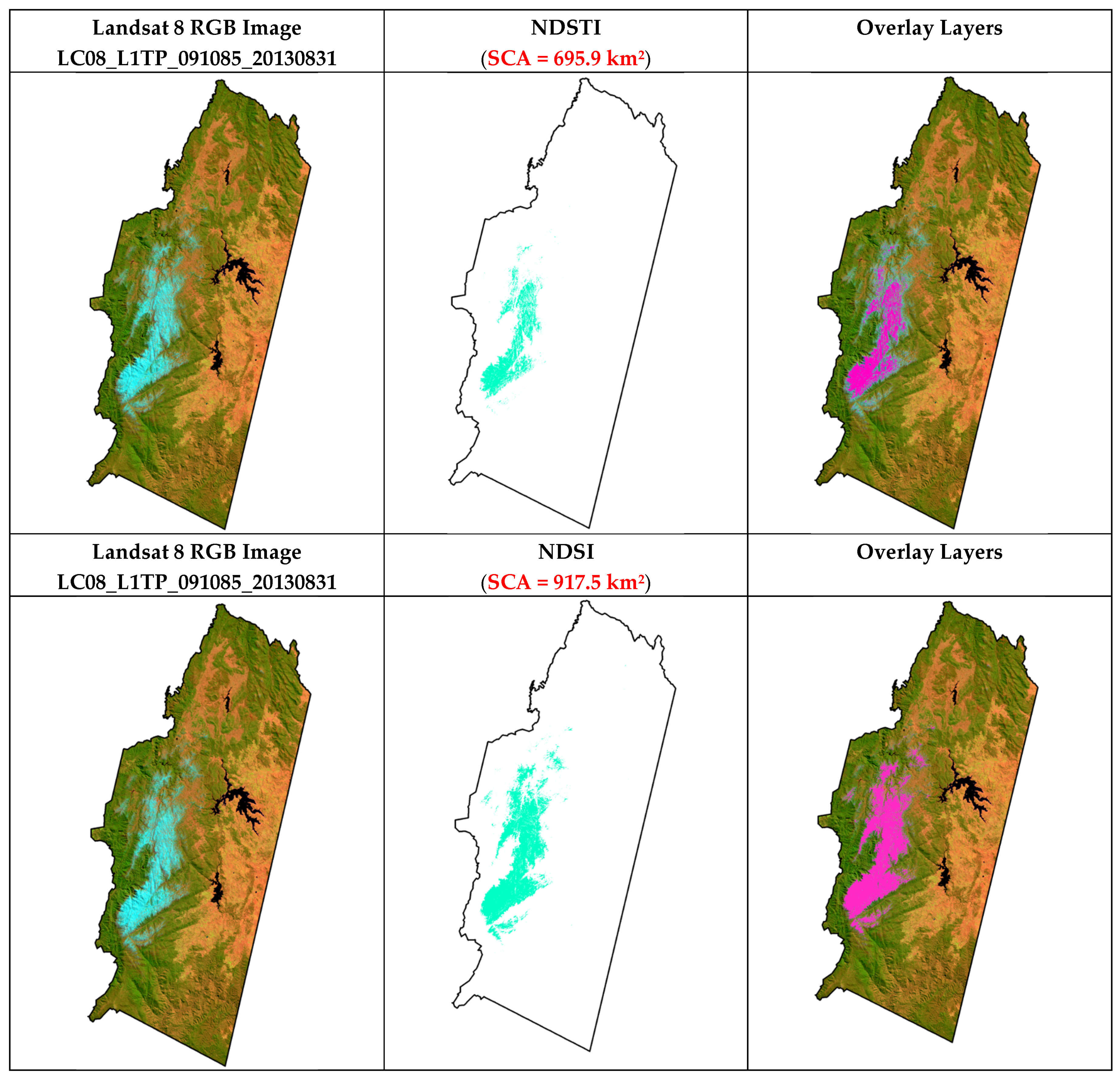
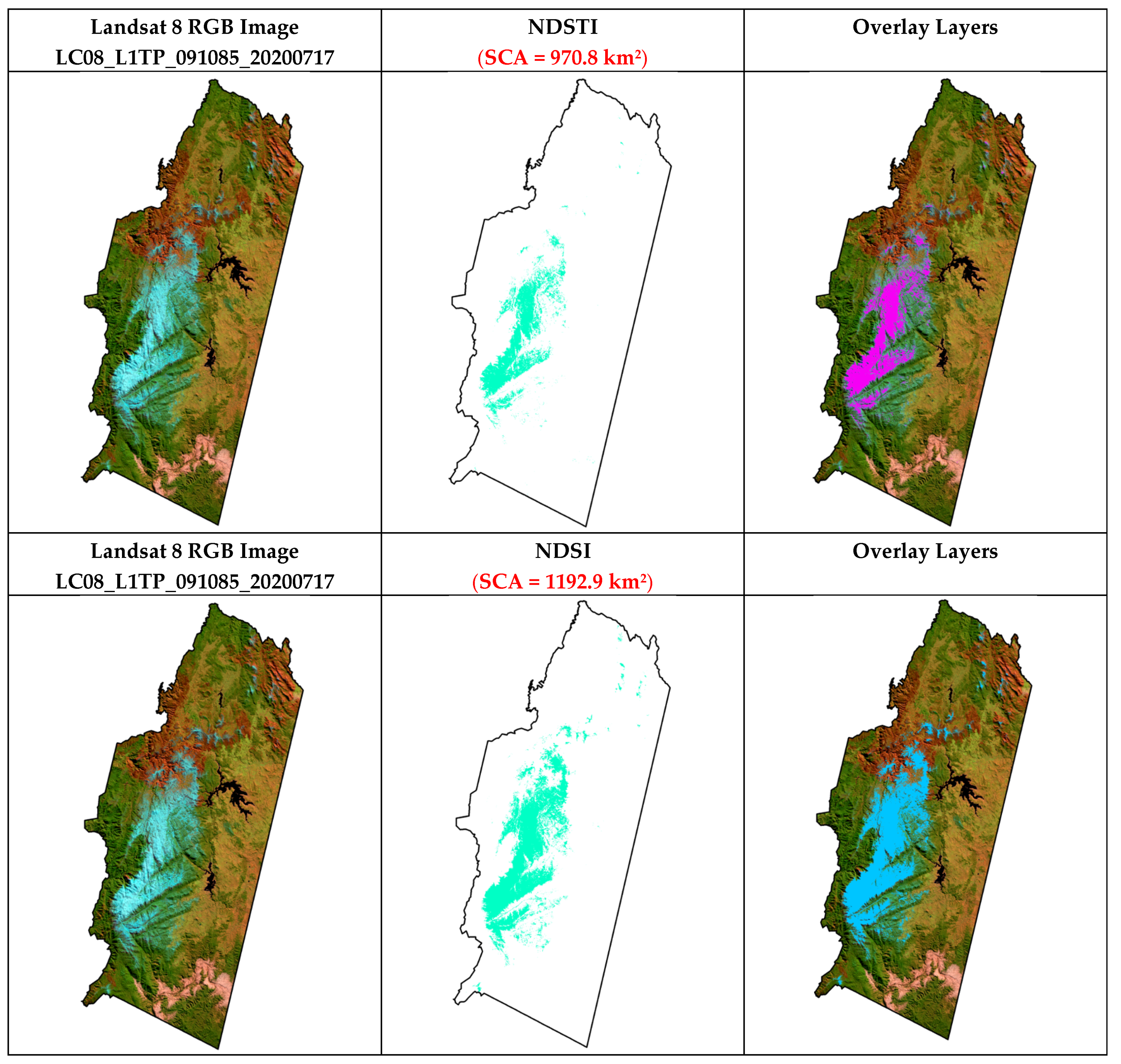
For comparison, we also applied the NDSTI to the Landsat 8 sampled images, only for 2013 and 2020. The NDSTI is defined as the difference of reflectance observed in a visible (blue) band (band-2, 0.452–0.512 µm) and Thermal Infrared (TIR) band (band-10, 10.600–11.190 µm) divided by the sum of the two reflectances: NDSTI = VIS (Blue) − TIR/VIS (Blue) + TIR. The index uses the spectral characteristics of snow/ice, a high reflectance in the visible region, and strong absorption in the TIR region. The index does not depend on reflectance in a single band [109]. Happily, we found that the proposed NDSTI is useful for identifying snow and ice and separating snow/ice from surrounding features. We also found that the thermal data are of great use in recognizing the boundary between snowy zones and non-snowy zones.
Despite all these advantages, the NDSTI has been used less than other remote sensing data for measuring snow characteristics. When we compared the results driven by NDSI and NDSTI, we found that NDSTI does not map water bodies as snow due to the coarser resolution of the Landsat Thermal band (Figure A4 and Figure A5). As can be seen from the comparison results of the relevant indices, in general, by applying the NDSTI, there is smaller SCA by about 18–20% in the final NDSTI products based on the 2013 and 2020 Landsat 8 image samples. We may conclude that further improvements are expected when higher-resolution thermal bands are available in the future.
Figure A4. The original Landsat 8 RGB image (left column), respective extracted snow maps by the NDSTI and NDSI (middle column), and the overlay layers (right column) for two times on the 31 August 2013.
Atmosphere 13 00826 g0a4
Figure A5. As in Figure A4, but for two times on the 17 July 2020.
Atmosphere 13 00826 g0a5

References

  1. Yang, D.; Robinson, D.; Zhao, Y.; Estilow, T.; Ye, B. Stream-flow response to seasonal snow cover extent changes in large Siberian watersheds. J. Geophys. Res. 2003, 108. [Google Scholar] [CrossRef]
  2. Zhou, X.; Li, S. Comparison between in situ and MODIS-derived spectral reflectances of snow and sea ice in the Amundsen Sea, Antarctica. Int. J. Remote Sens. 2003, 24, 5011–5032. [Google Scholar] [CrossRef]
  3. Bonan, G. Ecological Climatology, Concepts and Applications; Cambridge University Press: New York, NY, USA, 2002. [Google Scholar]
  4. Tong, J.; Velicogna, I. A Comparison of AMSR-E/Aqua Snow Products with in situ Observations and MODIS Snow Cover Products in the Mackenzie River Basin. Can. Remote Sens. 2010, 2, 2313–2322. [Google Scholar] [CrossRef] [Green Version]
  5. Löffler, J. Snow cover dynamics, soil moisture variability and vegetation ecology in high mountain catchments of central Norway. Hydrol. Processes 2005, 19, 2385–2405. [Google Scholar] [CrossRef]
  6. Isard, S.A.; Schaetzl, R.J.; Andresen, J.A. Soils cool as the climate warms in the great lakes region: 1951–2000. Ann. Assoc. Amer. Geog. 2007, 97, 467–476. [Google Scholar] [CrossRef]
  7. Lu, S.; Oki, K.; Omasa, K. Mapping snow cover using AVHRR/NDVI 10-day composite data. J. Agric. Meteorol. 2005, 60, 1215–1218. [Google Scholar] [CrossRef] [Green Version]
  8. Kargel, J.S.; Abrams, M.J.; Bishop, M.P.; Bush, A.; Hamiton, G.; Jiskoot, H.A.; Kieffer, H.H.; Lee, E.M.; Paul, F.; Rau, F.; et al. Multispectral imaging contributions to global land ice measurements from space. Remote Sens. Environ. 2005, 99, 187–219. [Google Scholar] [CrossRef]
  9. Chinn, H.; Salinger, J.; Fitzharris, B.; Willsman, A. Glaciers and climate. Bull. Fed. Mt. Clubs N. Z. 2008, 171, 1–15. [Google Scholar]
  10. Luca, A.D.; Evans, J.P.; Ji, F. Australian snowpack in NARCliM ensemble: Evaluation, bias correction and future projections. Clim. Dyn. 2018, 51, 639–666. [Google Scholar] [CrossRef]
  11. Davis, C.J. Meteorological aspects of snow. In Snow: A Natural History, an Uncertain Future; Green, K., Ed.; Australian Alps Liaison Committee: Canberra, Australia, 1998; pp. 3–34. [Google Scholar]
  12. Ruddell, A.R.; Budd, W.F.; Smith, I.N.; Keage, P.L.; Jones, R. The South-East Australian Alpine Climate Study; Meteorology Department, University of Melbourne for the Alpine Resorts Commission: Melbourne, VIC, Australia, 1990; p. 115. [Google Scholar]
  13. Department of the Environment, Water, Heritage, and the Arts, Australia. The Snowy Mountains Scheme; Culture and recreation portal: Canberra, ACT, Australia, 2008. [Google Scholar]
  14. Snowy-Hydro, Annual Report. In Snowy Hydro Limited and Its Controlled Entities; Snowy Valleys Council: Khancoban, NSW, Australia, 2020.
  15. Brown, B.D.; Braaten, R.O. Spatial and temporal variability of Canadian monthly snow depths, 1946–1995. Atmos. Ocean 1998, 36, 37–54. [Google Scholar] [CrossRef]
  16. Kavzoglu, T.; Colkesen, I. A kernel functions analysis for support vector machines for land cover classification. Int. J. Appl. Earth Obs. Geoinfo. 2009, 11, 352–359. [Google Scholar] [CrossRef]
  17. Foody, G.M. Status of land cover classification accuracy assessment. Remote Sens. Environ. 2002, 80, 185–201. [Google Scholar] [CrossRef]
  18. Gillanders, S.N.; Coops, N.C.; Wulder, M.A.; Gergel, S.E.; Nelson, T. Multitemporal remote sensing of landscape dynamics and pattern change: Describing natural and anthropogenic trends. Prog. Phys. Geog. 2008, 32, 503–528. [Google Scholar] [CrossRef]
  19. Stroeve, J.; Box, E.; Gao, F.; Liang, S.; Nolin, A.; Schaaf, C. Accuracy assessment of the MODIS 16-day albedo product for snow: Comparisons with Greenland in situ measurements. Remote Sens. Environ. 2005, 94, 46–60. [Google Scholar] [CrossRef]
  20. Foster, J.L.; Hall, D.K.; Chang, Z. Remote sensing of snow. Eos Trans. Amer. Geophys. Union 1987, 68, 682–684. [Google Scholar] [CrossRef]
  21. Foody, G.M. Land cover classification by an artificial neural network with ancillary information. Int. J. Remote Sens. 1995, 16, 527–542. [Google Scholar] [CrossRef]
  22. Köning, M.; Winther, J.G.; Isaksson, E. Measuring snow and glacier ice properties from satellite. Rev. Geophys. 2001, 39, 1–27. [Google Scholar] [CrossRef]
  23. Foppa, N.; Stoffel, A.; Meister, R. Synergy of in situ and space-borne observation for snow depth mapping in the Swiss Alps. Int. J. Appl. Earth Obs. Geoinf. 2007, 9, 294–310. [Google Scholar] [CrossRef]
  24. Shreve, C.M.; Okin, G.S.; Painter, T.H. Indices for estimating fractional snow cover in the western Tibetan Plateau. J. Glaciol. 2009, 55, 737–745. [Google Scholar] [CrossRef] [Green Version]
  25. Zhou, C.; Zheng, L. Mapping radar glacier zones and dry snow line in the Antarctic peninsula using sentinel-1 images. Remote Sens. 2017, 9, 1171. [Google Scholar] [CrossRef] [Green Version]
  26. Holroyd, E.W.; Verdin, J.P.; Carroll, T.R. Mapping snow cover with satellite imagery: Comparison of results from three sensor systems. In Proceedings of the 57th Annual Western Snow Conference, Fort Collins, CO, USA, 17–19 April 1989; pp. 59–68. [Google Scholar]
  27. Hall, D.K.; Kelly, R.E.J.; Foster, J.L.; Chang, A.T.C. Estimation of snow extent and snow properties. In Encyclopedia of Hydrological Sciences; Anderson, M.G., Ed.; Wiley: New York, NY, USA, 2005; pp. 811–828. [Google Scholar]
  28. Salomonson, V.V.; Appel, I. Estimating fractional snow-cover from MODIS using the normalized difference snow index. Remote Sens. Environ. 2004, 89, 351–360. [Google Scholar] [CrossRef]
  29. Salomonson, V.V.; Appel, I. Development of the Aqua MODIS NDSI fractional snow cover algorithm and validation results. IEEE Trans. Geosci. Remote Sens. 2006, 44, 1747–1756. [Google Scholar] [CrossRef]
  30. Aniya, M.; Sato, H.; Naruse, R.; Skvarca, P.; Casassa, G. The use of satellite and airborne imagery to inventory outlet glacier of Southern Patagonian Ice-field, South America. Photogramm. Eng. Remote Sens. 1996, 62, 1361–1369. [Google Scholar]
  31. Sidjak, R.W.; Wheate, R.D. Glacier mapping of the Illecillewaet ice-field, British Columbia, Canada, using Landsat TM and digital elevation data. Int. J. Remote Sens. 1999, 20, 273–284. [Google Scholar] [CrossRef]
  32. Corripio, J.G. Snow surface albedo estimation using terrestrial photography. Int. J. Remote Sens. 2004, 25, 5705–5729. [Google Scholar] [CrossRef]
  33. Andreassen, L.; Paul, F.; Kääb, A.; Hausberg, J. Landsat-derived glacier inventory for Jotunheimen, Norway, and deduced glacier changes since the 1930s. Cryosphere 2008, 2, 131–145. [Google Scholar] [CrossRef] [Green Version]
  34. Xiao, X.; Moore, B.; Qin, X.; Shen, Z.; Boles, S. Large-scale observations of alpine snow and ice cover in Asia: Using multi-temporal VEGETATION sensor data. Int. J. Remote Sens. 2002, 23, 2213–2228. [Google Scholar] [CrossRef] [Green Version]
  35. Gascoin, S.; Grizonnet, M.; Bouchet, M.; Salgues, G.; Hagolle, O. Theia Snow collection: High-resolution operational snow cover maps from Sentinel-2 and Landsat-8 data. Earth Syst. Sci. Data 2019, 11, 493–514. [Google Scholar] [CrossRef] [Green Version]
  36. Bronge, L.B.; Bronge, C. Ice and snow type classification in Vestfold Hills, East Antarctica, using LANDSAT TM data and ground radiometer measurements. Int. J. Remote Sens. 1999, 20, 225–240. [Google Scholar] [CrossRef]
  37. Bolch, T.; Menounos, B.; Wheate, R. Landsat-based inventory of glaciers in western Canada, 1985–2005. Remote Sens. Environ. 2010, 114, 127–137. [Google Scholar] [CrossRef]
  38. Hellesen, T.; Matikainen, L. An object-based approach for mapping shrub and tree cover on grassland habitats by use of LiDAR and CIR orthoimages. Remote Sens. 2013, 5, 558–583. [Google Scholar] [CrossRef] [Green Version]
  39. Teodoro, A.C.; Araújo, R. Exploration of the OBIA methods available in SPRING noncommercial software to UAV data processing. Proceeding SPIE Int. Soc. Opt. Eng. 2014, 9245, 92451F. [Google Scholar] [CrossRef]
  40. Tiede, D.; Krafft, P.; Füreder, P.; Lang, S. Stratified Template Matching to Support Refugee Camp Analysis in OBIA-Workflows. Remote Sens. 2017, 9, 326. [Google Scholar] [CrossRef] [Green Version]
  41. Blaschke, T. Object-based image analysis for remote sensing. ISPRS J. Photogramm. Remote Sens. 2010, 65, 2–16. [Google Scholar] [CrossRef] [Green Version]
  42. Hay, G.J.; Castilla, G. Object-based Image Analysis, Strengths, weaknesses, opportunities, and threats (SWOTs). In OBIA International Archives of Photogrammetry, Remote Sensing, and Spatial Information Sciences; ISPRS: Hannover, Germany, 2006. [Google Scholar]
  43. Kato, L. Integrating Open-street map Data. In Object-Based Land-Cover and Land-Use Classification for Disaster Recovery; LAP LAMBERT Academic Publishing: Chisinau, Republic of Moldova, 2020; p. 76. [Google Scholar]
  44. Drǎguţ, L.; Tiede, D.; Levick, S.R. ESP: A tool to estimate scale parameter for multiresolution image segmentation of remotely sensed data. Int. J. Geog. Inf. Sci. 2010, 24, 859–871. [Google Scholar] [CrossRef]
  45. eCognition Reference Book, eCognition Developer for Windows Operating System, Version 9.5.1; Trimble: Sunnyvale, CA, USA, 2019.
  46. NSW-NPWS. Kosciuszko Walk—Thredbo to Mount Kosciuszko; National Parks and Wildlife Service: Parramatta, NSW, Australia, 2014. [Google Scholar]
  47. Bureau of Meteorology. Climate Glossary; Australian Federal Government: Canberra, ACT, Australia, 2015. [Google Scholar]
  48. Stern, H.; de Hoedt, G.; Ernst, J. Objective Classification of Australian Climates; Australian Bureau of Meteorology: Melbourne, VIC, Australia, 2000. [Google Scholar]
  49. Costin, A.B. Kosciusko Alpine Flora, 1st ed.; CSIRO Publishing: Clayton, VIC, Australia, 1979. [Google Scholar]
  50. NSW-NPWS. Kosciuszko National Park Plan of Management, 2nd ed.; National Parks and Wildlife Service: Hurstville, NSW, Australia, 1988. [Google Scholar]
  51. Slatyer, R.O.; Cochrane, P.M.; Galloway, R.W. Duration and extent of snow cover in the Snowy Mountains and a comparison with Switzerland. Search 1984, 11–12, 327–331. [Google Scholar]
  52. Edmonds, T.; Lunt, I.D.; Roshier, D.A.; Louis, J. Annual variation in the distribution of summer snowdrifts in the Kosciuszko alpine area, Australia, and its effect on the composition and structure of alpine vegetation. Austral Ecol. 2006, 31, 837–848. [Google Scholar] [CrossRef]
  53. Abrams, M.; Bailey, B.; Tsu, H.; Hato, M. The ASTER Global DEM. J. Am. Soc. Photog. Remote Sens. 2010, 20, 344–348. [Google Scholar]
  54. U.S. Geological Survey. Landsat Analysis Ready Data: U.S. Geological Survey Fact Sheet; U.S. Geological Survey: Reston, VA, USA, 2018.
  55. Woodcock, C.E.; Allen, R.; Anderson, M.; Belward, A.; Bindschadler, R.; Cohen, W.; Gao, F.; Goward, S.N.; Helder, D.; Helmer, E. Free Access to Landsat Imagery. Science 2008, 320, 1011. [Google Scholar] [CrossRef]
  56. Jensen, J.R. Introductory Digital Image Processing, a Remote Sensing Perspective, 3rd ed.; Pearson Education, Inc.: Upper Saddle River, NJ, USA, 2005; p. 526. [Google Scholar]
  57. Alparone, L.; Aiazzi, B.; Baronti, S.; Garzelli, A. Remote Sensing Image Fusion (Signal and Image Processing of Earth Observations), 1st ed.; CRC Press: Boca Raton, FL, USA, 2015. [Google Scholar]
  58. Dedopulos, T. Earth View: Extraordinary Images of Our Planet from the Landsat NASA/USGS Satellites; Carlton Books: London, UK, 2019. [Google Scholar]
  59. Baatz, M.; Schäpe, A. Multiresolution segmentation—An optimization approach for high quality multi-scale image segmentation. In Angewandte Geographische Information Severer Beitung; Strobl, J., Blaschke, T., Griesebner, G., Eds.; Wichmann-Verlag: Heidelberg, Germany, 2000; pp. 12–23. [Google Scholar]
  60. Burnett, C.; Blaschke, T. A multi-scale segmentation/object relationship modeling methodology for landscape analysis. Ecol. Model. 2003, 168, 233–249. [Google Scholar] [CrossRef]
  61. eCognition Reference Book. In Trimble eCognition® Reference Book; Trimble Germany GmbH: Munich, Germany, 2014.
  62. Dozier, J. Spectral signature of alpine snow cover from the Landsat Thematic Mapper. Remote Sens. Environ. 1989, 28, 9–22. [Google Scholar] [CrossRef]
  63. Riggs, G.A.; Hall, D.K.; Salomonson, V.V. A snow index for the Landsat thematic mapper and moderate resolution imaging spectroradiometer. In Proceedings of the International Geoscience and Remote Sensing Symposium, IGARSS ‘94, Pasadena, CA, USA, 8–12 August 1994; pp. 1942–1944. [Google Scholar]
  64. Shimamura, Y.; Izumi, T.; Matsumaya, H. Evaluation of a useful method to identify snow-covered areas under vegetation—Comparisons among a newly proposed snow index, normalized difference snow index and visible reflectance. Int. J. Remote Sens. 2006, 27, 4867–4884. [Google Scholar] [CrossRef]
  65. Manandhar, R.; Odeh, I.O.; Ancev, T. Improving the accuracy of landuse and land cover classification of Landsat data using post-classification enhancement. Remote Sens. 2009, 1, 330–344. [Google Scholar] [CrossRef] [Green Version]
  66. Rasouli, A.A.; Milani, M.; Milan, B. Mastering Object-Based Image Analysis: To Imaging the Azerbaijan Geo-Environment; iKSAD Publishing House: Ankara, Turkey, 2021. [Google Scholar]
  67. Snowy Hydro, Home to our diesel assets. In Australian Hydro Projects: Operating, Energy News Bulletin; Aspermont Ltd.: Perth, WA, Australia, 2018.
  68. Pepler, A.S.; Trewin, B.; Ganter, C. The influences of climate drivers on the Australian snow season. Aust. Meteorol. Oceanogr. J. 2015, 65, 195–205. [Google Scholar] [CrossRef]
  69. Molotch, N.P.; Margulis, S.A. Estimating the distribution of snow water equivalent using remotely sensed snow cover data and a spatially distributed snowmelt model: A multi-resolution, multi-sensor comparison. Adv. Water Resour. 2008, 31, 1503–1514. [Google Scholar] [CrossRef]
  70. Hennessy, K.J.; Whetton, P.H. Snow-Making and Greenhouse Warming at Falls Creek and Mt Hotham, Australia; Falls Creek Ski Lifts Pty Ltd and Mt Hotham Skiing Company Pty Ltd, Climate Impact Group, CSIRO Atmospheric Research: Melbourne, VIC, Australia, 2001; p. 20. [Google Scholar]
  71. Matthews, A.; Spooner, P.G.; Lunney, D.; Green, K.; Klomp, N.I. The influences of snow cover, vegetation and topography on the upper range limit of common wombats Vombatus Ursinus in the subalpine zone, Australia. Divers. Distrib. 2010, 16, 277–287. [Google Scholar] [CrossRef]
  72. Zhong, X.; Zhang, T.; Kang, S.; Wang, J. Snow depth trends from CMIP6 models conflict with observational evidence. J. Clim. 2021, 35, 1293–1307. [Google Scholar] [CrossRef]
  73. IPCC. Climate Change 2021: The Physical Science Basis; Contribution of Working Group I to the Sixth Assessment Report of the Intergovernmental Panel on Climate Change; Masson-Delmotte, V., Zhai, P., Pirani, A., Connors, S.L., Péan, C., Berger, S., Caud, N., Chen, Y., Goldfarb, L., et al., Eds.; Cambridge University Press: London, UK, 2021. [Google Scholar]
  74. Hennessy, K.; Whetton, P.; Smith, I.; Bathols, J.; Hutchinson, M.; Sharples, J. The Impact of Climate Change on Snow Conditions in Mainland Australia; CSIRO Atmospheric Research: Melbourne, VIC, Australia, 2003. [Google Scholar]
  75. Matiu, M.; Crespi, A.; Bertoldi, G.; Carmagnola, C.M.; Marty, C.; Morin, S.; Schöner, W.; Berro, D.C.; Chiogna, G.; De Gregorio, L.; et al. Observed snow depth trends in the European Alps: 1971 to 2019. Cryosphere 2021, 15, 13431382. [Google Scholar] [CrossRef]
  76. Andersen, T. Operational snow mapping by satellites. In Hydrological Aspects of Alpine and High Mountain Areas, Proceedings of the Exeter Symposium; IAHS Publish: Wallingford, UK, 1982; Volume 138, pp. 149–154. [Google Scholar]
  77. Wang, J.; Li, W. Comparison of methods of snow cover mapping by analyzing the solar spectrum of satellite remote sensing data in China. Int. J. Remote Sens. 2003, 24, 4129–4136. [Google Scholar] [CrossRef]
  78. Gri, D.; Hay, G. Integrating GEOBIA, Machine Learning, and Volunteered Geographic Information to Map Vegetation over Rooftops. ISPRS Int. J. Geo-Inf. 2018, 7, 462. [Google Scholar]
  79. Whitesidea, T.G.; Boggs, G.S.; Maier, S.W. Comparing object-based and pixel-based classifications for mapping savannas. Int. J. Appl. Earth Obs. Geoinf. 2011, 13, 884–893. [Google Scholar] [CrossRef]
  80. Tanimoto, S.L. An Interdisciplinary Introduction to Image Processing: Pixels, Numbers, and Programs; The MIT Press: Boston, MA, USA, 2012. [Google Scholar]
  81. Ranchin, T.; Wald, L. Fusion of high spatial and spectral resolution images: The ARSIS concept and its implementation. Photogramm. Eng. Remote Sens. 2000, 66, 49–61. [Google Scholar]
  82. Navulur, K. Multispectral Image Analysis Using the Object-Oriented Paradigm (Remote Sensing Applications Series), 1st ed.; CRC Press: Boca Raton, FL, USA, 2020; p. 204. [Google Scholar]
  83. Guirado, E.; Tabik, S.; Alcaraz-Segura, D.; Cabello, J.; Herrera, F. Deep-learning versus OBIA for scattered shrub detection with Google Earth imagery: Ziziphus lotus as a case study. Remote Sens. 2017, 9, 1220. [Google Scholar] [CrossRef] [Green Version]
  84. Sanchez-Espinosa, A.; Schroder, C. Land use and land cover mapping in wetlands one step closer to the ground: Sentinel-2 versus Landsat 8. J. Environ. Manag. 2019, 247, 484–498. [Google Scholar] [CrossRef] [PubMed]
  85. Rasouli, A.A.; Safarov, S.H.; Asgarova, M.M.; Safarov, E.S.; Milani, M. Detectıon and Mappıng of Green-Cover and Landuse Changes by Advanced Satellıte Image Processıng Technıques; A Case Study: Azerbaijan Eastern Zangezur Economic Region; ANAS Transactions; Earth Sciences: Baku, Azerbaijan, 2021; p. 18. [Google Scholar]
  86. Green, K.; Pickering, C.M. The Decline of Snow patches in the Snowy Mountains of Australia: Importance of Climate Warming, Variable Snow, and Wind. Arct. Antarct. Alp. Res. Interdiscip. J. 2009, 41, 212–218. [Google Scholar] [CrossRef] [Green Version]
  87. Clifford, D. Global estimates of snow water equivalent from passive microwave instruments: History, challenges, and future developments. Int. J. Remote Sens. 2010, 31, 3707–3726. [Google Scholar] [CrossRef]
  88. Bilish, S.P.; Callow, J.N.; McGrath, G.S.; McGowan, H.A. Spatial controls on the distribution and dynamics of a marginal snowpack in the Australian Alps. Hydrol. Process 2019, 33, 1739–1755. [Google Scholar] [CrossRef]
  89. Tsang, L.; Durand, M.; Derksen, C.; Barros, A.P.; Kang, D.H.; Lievens, H.; Marshall, H.; Zhu, J.; Johnson, J.; King, J.; et al. Global monitoring of snow water equivalent using high frequency radar remote sensing. Cryosphere 2021, 1–57. [Google Scholar] [CrossRef]
  90. Barnett, T.P.; Adam, J.C.; Lettenmaier, D.P. Potential impact of a warming climate on water availability in snow-dominated regions. Nature 2005, 438, 303–309. [Google Scholar] [CrossRef]
  91. Li, D.; Wrzesien, M.L.; Durand, M.; Adam, J.; Lettenmaier, D.P. How much runoff originates as snow in the western United States, and how will that change in the future? Geophys. Res. Lett. 2017, 44, 6163–6172. [Google Scholar] [CrossRef] [Green Version]
  92. Beniston, M.; Farinotti, D.; Stoffel, M.; Andreassen, L.M.; Coppola, E.; Eckert, N.; Fantini, A.; Giacona, F.; Hauck, C.; Huss, M.; et al. The European mountain cryosphere: A review of its current state, trends, and future challenges. Cryosphere 2018, 12, 759–794. [Google Scholar] [CrossRef] [Green Version]
  93. Klein GVitasse, Y.; Rixen, C.; Marty, C.; Rebetez, M. Shorter snow cover duration since 1970 in the Swiss Alps due to earlier snowmelt more than to later snow onset. Clim. Change 2016, 139, 637–649. [Google Scholar] [CrossRef]
  94. Notarnicola, C. Hotspots of snow cover changes in global mountain regions over 2000–2018. Remote Sens. Environ. 2020, 243, 111781. [Google Scholar] [CrossRef]
  95. Trimble eCognition Suite. eCognition Developer 10.2 Reference Book; Trimble Documentation: Munich, Germany, 2021. [Google Scholar]
  96. Nilsson, S. A Review of Assessing the Accuracy of Classifications of Remotely Sensed Data and of Methods Including Remote Sensing Data in Forest Inventory; International Institute for Applied Systems Analysis: Ladenburg, Austria, 1998; Volume A-2361. [Google Scholar]
  97. Hellden, U. A Test of Landsat-2 Imagery and Digital Data for Thematic Mapping Illustrated by an Environmental Study in Northern Kenya; Lund University National Geographic Institute: Lund, Sweden, 1980; p. 47. [Google Scholar]
  98. Short, N.M. The Landsat Tutorical Workbook—Basics of Satellite Remote Sensing; Goddard Space Flight Center: Greenbelt, MD, USA, 1982; p. 1078. [Google Scholar]
  99. Brennan, R.; Prediger, D. Coefficient Kappa: Some Uses, Misuses and Alternatives. Educ. Psychol. Meas. 1981, 41, 687–699. [Google Scholar] [CrossRef]
  100. Motoya, K.; Saito, A.; Mabuchi, A.; Aoki, T.; Yamazaki, T. Application to the Airborne Multi-Spectral Scanner (AMSS) observation in 1998 of the vegetation and snow indices, based on the spectral reflectance characteristic. J. Jpn. Soc. Hydrol. Water Resour. 2001, 14, 239–245. [Google Scholar] [CrossRef] [Green Version]
  101. Asaoka, Y.; Kazama, S.; Sawamoto, M. The variation characteristics of snow water resources in a wide area and its geographical and climatic dependency. J. Jpn. Soc. Hydrol. Water Resour. 2002, 15, 279–289. [Google Scholar] [CrossRef] [Green Version]
  102. Bitner, D.; Carrollg, T.; Cline, D.; Romanov, P. An assessment of the differences between three satellite snow cover mapping techniques. Hydrol. Processes 2002, 16, 3723–3733. [Google Scholar] [CrossRef]
  103. Hall, D.K.; Riggs, G.A.; Salomonson, V.V. Development of methods for global mapping snow-cover using moderate resolution spectroradiometer data. Remote Sens. Environ. 1995, 54, 127–140. [Google Scholar] [CrossRef]
  104. Bormann, K.J.; McCabe, M.F.; Evans, J.P. Satellite-based observations for seasonal snow cover detection and characterization in Australia. Remote Sens. Environ. 2012, 123, 57–71. [Google Scholar] [CrossRef]
  105. Xiao, X.; Shen, Z.; Qin, X. Assessing the potential of VEGETATION sensor data for mapping snow and ice cover: A normalized difference snow and ice index. Int. J. Remote Sens. 2001, 22, 2479–2487. [Google Scholar] [CrossRef]
  106. Saydi, M.; Li, D.J. Impacts of topographic factors on regional snow cover characteristics. Water Sci. Eng. 2020, 13, 171–180. [Google Scholar] [CrossRef]
  107. Sibandze, P.; Mhangara, P.; Odindi, J.; Kganyago, M. A comparison of Normalized Difference Snow Index (NDSI) and Normalized Difference Principal Component Snow Index (NDPCSI) techniques in distinguishing snow from related land cover types. South Afr. J. Geomat. 2014, 3, 197. [Google Scholar] [CrossRef] [Green Version]
  108. Haq, M.A.; Jain, K.; Menon, K.P.R. Development of New Thermal Ratio Index for Snow/Ice Identification. Int. J. Soft Comput. Eng. 2012, 1, 2231–2307. [Google Scholar]
  109. Tong RParajka, J.; Komma, J.; Blöschl, G. Mapping snow cover from daily Collection 6 MODIS products over Austria. J. Hydrol. 2020, 590, 125548. [Google Scholar] [CrossRef]
  110. Rasouli, A.A.; Mammadov, R. Preliminary Satellite Image Analysis Inside the ArcGIS Setting; Lambert Academy Publishing: Chisinau, Republic of Moldova, 2020. [Google Scholar]
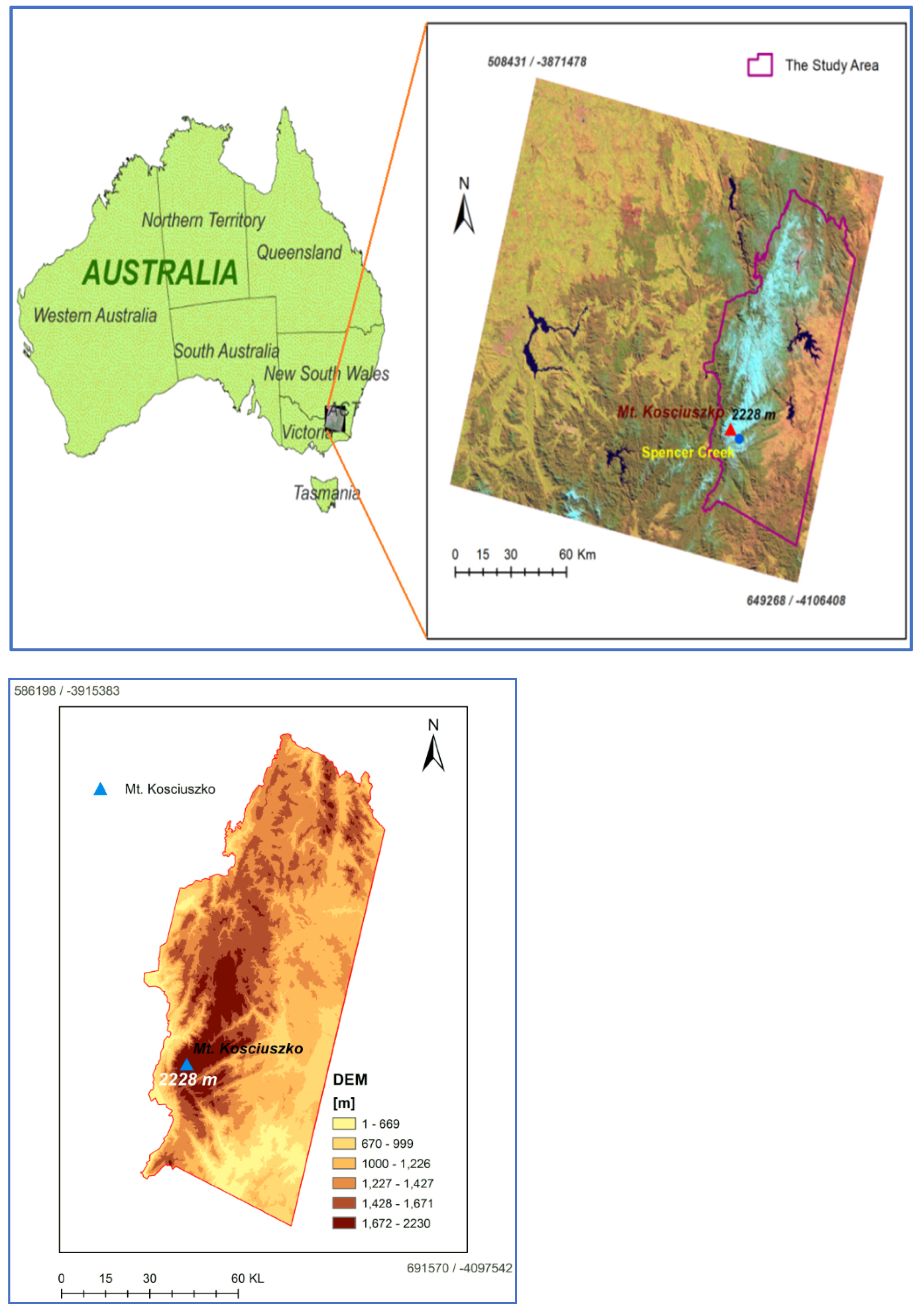
Figure 1. The location of the Snowy Mountains in Australia (upper) and topographic map of the study area (lower).
Atmosphere 13 00826 g001
Figure 2. A sample Landsat image with maximum snow cover and a few well-recognized geographic features, adjusted to the study area boundary.
Atmosphere 13 00826 g002
Figure 3. Illustration of the selection of an optimal scale parameter of multi-resolution segmentation based on Landsat imagery information. Graphs depict changes in local variance (LV) (red dots) and rate of change (blue dots) with increasing scale parameters. Vertical green boxes indicate optimal (critical) scale parameters selected for each scene.
Atmosphere 13 00826 g003
Figure 4. Interannual time series of the observed MSDs at the three snow observations sites. The linear regression line for each site with explained variance is shown.
Atmosphere 13 00826 g004
Figure 5. The sequence of generation of the indices NDSI (snow), SWI (water), and NDVI (vegetation) in comparison to the RGB image to the right.
Atmosphere 13 00826 g005
Figure 6. The temporal–spatial variations of the annual maximum SCA inside the Snowy Mountains area from 1984 to 2020. The MSD and SCA for each year are shown in each panel. The minimum, average, and maximum SCAs are 417.7, 1003.6, and 1774.7 km2. The standard deviation is 308.3 km2 and the skewness is 0.5.
Atmosphere 13 00826 g006aAtmosphere 13 00826 g006b
Figure 7. Time series of the maximum value of SCA in each year of the study period (solid line). The month of the maximum value has been labelled. The dashed line represents the 3-year running mean.
Atmosphere 13 00826 g007
Table 1. A set of equations applied when implementing dynamic rule-based procedures.
IndexEquationCondition
NDV I Landsat   5   &   7 ( NI R b 4 RE D b 3 ) / ( NI R b 4 + RE D b 3 ) Equation (1)
If Mean NDVI ≥ 0.32 and Brightness ≤ 38, it is vegetation
NDV I Landsat   8 ( NI R b 5 RE D b 4 ) / ( NI R b 5 + RE D b 4 )
SW I Landsat   5 ,   7   &   8 ( ( BlUE × 0.2626 ) + ( GREEN × 0.2141 ) + ( RED × 0.0926 ) + ( NIR × ( 0.0656 ) ) + ( MIR × ( 0.7629 ) ) + ( SWIR × ( 0.5388 ) ) Equation (2)
If SWI ≥ 1100, NDVI ≤ 0, and Area ≥ 10000 Pxl, it is water
NDS I Landsat   5   &   7 ( Green   b 2 NI R b 5 ) / ( Green   b 2 + NI R b 5 ) Equation (3)
If Mean Layer 1 ≥ 155, NDSI ≤ 0, and Brightness ≥ 83, it is snow
NDS I Landsat   8 ( Green   b 3 NI R b 6 ) / ( Green   b 3 + NI R b 6 )
SWI—Surface Water Index; NIR—Near Infrared; MIR—Middle Infrared; SWIR—Short-Wave Infrared.
Table 2. MSD frequency during the cold months and linear correlation coefficients among the three SD observations sites.
Observing
Station
Cold Months MSD FrequencyCorrelation among SitesCorrelation between Sites and SCA
JunJulAugSepOctTotal
Spencers Creek032012237
Deep Creek172270370.86 (SC and DC)0.28 (SC and SCA)
Three Mile Dam4131640370.55 (SC and TM)0.38 (DC and SCA)
Total52582121090.80 (DC and TM)0.29 (TM and SCA)
Percentage4.621.153.219.31.8100
Table 3. The accuracy assessment process results for snow, water, vegetation, and other classes. The upper part shows the confusion matrix; the lower part shows the accuracy measures.
User/ReferenceSnowWaterVegetationOther ClassesSum
Confusion Matrix
Snow47270004727
Water08615008615
Vegetation0011264012,040
Others2550065946849
Sum49828615112647370
Accuracy
Producer0.948110.894
User110.9350.962
Hellden0.97910.9660.927
Short0.9410.9350.864
KIA Per Class0.95110.866
Totals
Overall accuracy = 0.968
KIA = 0.956
Publisher’s Note: MDPI stays neutral with regard to jurisdictional claims in published maps and institutional affiliations.