Short-Term Canyon Wind Speed Prediction Based on CNN—GRU Transfer Learning

Abstract

Due to the particularity of the site selection of hydropower stations, the canyon wind with large fluctuations often occurs during the construction of the hydropower station, which will seriously affect the safety of construction personnel. Especially in the early stage of the construction of the hydropower station, the historical data and information on the canyon wind are scarce. Short-term forecasting of canyon wind speed has become extremely important. The main innovation of this paper is to propose a time series prediction method based on transfer learning. This method can achieve short-term prediction when there are few wind speed sample data, and the model is relatively simple while ensuring the accuracy of prediction. Considering the temporal and nonlinear characteristics of canyon wind speed data, a hybrid transfer learning model based on a convolutional neural network (CNN) and gated recurrent neural network (GRU) is proposed to predict short-term canyon wind speed with fewer observation data. In this method, the time sliding window is used to extract time series from historical wind speed data and temperature data of adjacent cities as the input of the neural network. Next, CNN is used to extract the feature vector from the input, and the feature vector can form time series. Then, the GRU network is used for short-term wind speed prediction by the time series. Experimental results show that the proposed method improves MAE and RMSE by nearly 20%, which will provide new ideas for the application of wind speed forecasting in canyons under complex terrain. The research contents of this paper contribute to the actual construction of hydropower stations.

1. Introduction

Hydropower is an important part of China’s energy, which can provide about 1/4 of China’s electricity supply [1]. The development of hydropower can not only provide electricity, but also has comprehensive social benefits such as flood control, irrigation, tourism, and promote regional economic development [2,3]. Hydroelectric power generation is realized by converting the potential energy contained in the high rivers and lakes into the kinetic energy of the hydraulic turbine, and then pushing the generator to generate electric energy [4,5]. Based on the power generation principle of hydropower stations, hydropower dams are generally built in canyons with large river drops and complex terrain. However, it is inevitable to consider the impact of canyon wind when building hydropower stations in a canyon with large terrain drops [6]. Strong winds in the canyon can directly affect the construction of hydropower stations, and the safety of workers and can cause immeasurable losses [7]. For example, the Baihetan Hydropower Station, located at the junction of the Qinghai-Tibet Plateau and the Chengdu Plain, has a complex topography and a changeable climate. Since the construction of this station started, strong winds have occurred frequently. According to historical data, 235 days of strong winds above level 7 occur each year, accounting for 64.2% of the whole year. This poses a serious challenge to the construction progress and safety of the dam during the pouring period. In the early stage of hydropower dam construction, historical wind speed data at construction sites were particularly scarce and there were many missing values in the data. It is even more difficult to qualitatively analyze wind speed characteristics. In response to these thorny issues, it is of great practical significance to study canyon wind speed prediction, which can provide technical support for engineering construction quality and safety, reduce risk, and control cost management [8].

In recent years, both domestic and foreign scholars have carried out a lot of research on wind speed prediction and proposed a variety of methods. In general, these methods can be divided into three categories [9]: (1) Physical models: This type of method uses physical factors, and meteorological data including terrain, pressure, and temperature to estimate future wind speeds [10]. Sometimes they are just the first step in the prediction, as an auxiliary input to other statistical models. Numerical Weather Prediction (NWP) is a method proposed to solve weather forecasting problems by meteorologists. To represent the local terrain, a digital elevation model can be used in the NWP to obtain more accurate results. Landberg proposed an automated online prediction system in which the NWP model was also used [11]. Since NWP is a large-scale prediction model, when the research object is a specific wind farm, other detailed information such as terrain and roughness is needed. The simplest method of wind speed prediction is a continuous method [12]. This method takes the nearest wind speed observation as the next point for forecast and greatly improves the prediction effect of wind speed in the next 6 h. However, this method can only make short-term predictions. Negnevitsky et al., pointed out that NWP models should introduce accurate digital elevation and the output data to correct short-term forecasts [13]. However, the disadvantage of the physical model is also obvious, that is, any certain physical model cannot well simulate the real wind speed data, which will greatly reduce the accuracy of wind speed prediction. (2) Traditional statistical model: This type of method is based on the correlation of wind speed series and establishes a predictive model through steps including model identification, parameter estimation, and model verification. It describes the changes in historical wind speed series and then predicts future changes. Its common modeling methods mainly include the Autoregressive model (AG), Moving Average model (MA), Autoregressive Moving Average model (ARMA), and Regressive Integrated Moving Average model (ARIMA) [14]. Lalarukh and Yasmin proposed a model involving self-correlation, non-Gaussian distribution, and daily non-stable [15]. Torres et al., used the ARMA model to predict average wind speed in hours and pointed out that the transformation and standardization of time series are very important. Costa et al., used Kalman filtering to predict wind speed and the experimental results showed that it is better for predicting wind speed by a five-minute step [16]. However, the disadvantage of traditional statistical methods is that those methods have a poor fitting effect on nonlinear data sets, those methods are not ideal for identifying complex data, and are easy to cause over-fitting because traditional statistical models do not have a learning process. (3) Artificial intelligence model: Now, with the development of artificial intelligence and other prediction methods, a variety of new models for wind speed and wind power prediction have been proposed. These include Support Vector Machines (SVM) [17], Fuzzy Logic methods [18], Artificial Neural Networks (ANN) [19], and hybrid prediction methods. Monhandes et al., used SVM for wind speed prediction and compared it with multi-layer Perceptron neural networks (MLP) [20]. The results showed that the SVM model has a lower prediction error than MLP. Ji et al., also proposed a support vector classifier for estimating prediction errors [21]. Sancho et al., proposed a progressive support vector regression method to solve parameter estimation problems in SVM based on iterative techniques [22]. Zhou et al., systematically studied the selection of the least-square-SVM parameters by using three SVM cores involving linear, Gaussian, and polynomial [23]. Hu et al., analyzed the different noises of support vector machines to complete the prediction modeling [24]. Fuzzy Logic methods use a linear model to approximate the nonlinear dynamic wind speed changes by a database of fuzzy rules with data and language based on fuzzy logic and the expertise of forecasters [25]. Due to the weak learning ability of fuzzy prediction, the effect of the pure fuzzy method is often not good. The selection of the structure of the fuzzy system requires further research. Thus, the fuzzy prediction method is usually used in conjunction with other methods. For example, Siderotos and Hatziargyriou proposed a fuzzy method, which is combined with a neural network and obtained satisfactory results [26]. However, the common problem of deep learning is that it is not suitable for solving a class of problems, which will lead to wind speed prediction in a different scene, so it is necessary to reconstruct the model, which is time-consuming and laborious.

The above methods have their characteristics, but they all meet the premise of sufficient wind speed data. However, it is often difficult to learn a good prediction model for wind speed prediction due to insufficient data on new wind farms or engineering construction. Togelou et al., proposed a self-constructed and adaptive statistical model for this problem [27], but this model is complicated to establish and does not use other available wind speed data. At this point, we consider borrowing appropriate wind speed data directly from the area around the hydropower station to assist in modeling. Therefore, we introduce a modeling strategy of transfer learning (TL) [28]. Transfer learning can complete short-term wind speed prediction under the condition of a few sample data by applying the knowledge learned in certain fields. This strategy can learn a shared model from the data of different domains and then fine-tune the shared model to obtain a unique mathematical model to better complete the prediction.

This study is the first study due to its ability both to deal effectively with the nonlinear problem and to make high accuracy for small sample data in wind speed time series. The main contributions presented in this study are as follows:

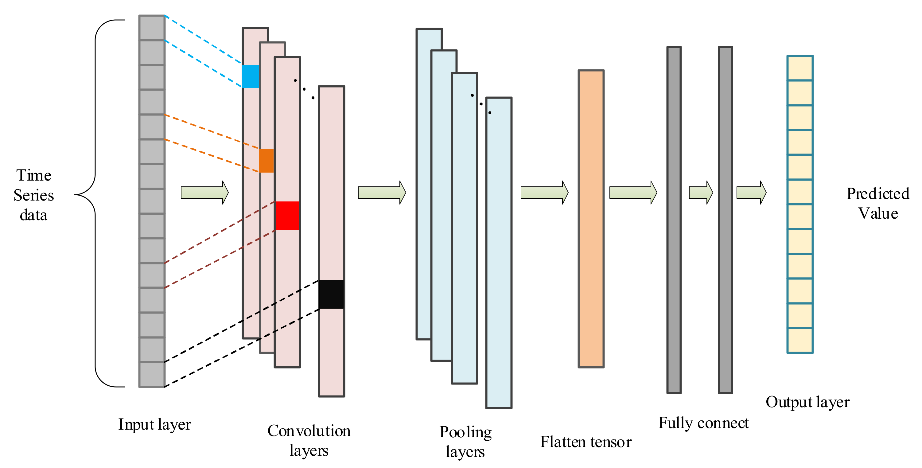
• This paper proposed a CNN—GRU method to predict short-term canyon wind speed for the time series and nonlinear characteristics of any wind speed. This model constructs a multi-layer convolutional neural network to extract the complex features of wind speed and GRU model is used to learn the relationship between time series, this model solves the difficulty of extracting high-level features of wind speed data and the gradient disappearing when the model learns time-series information. Through this method, the wind speed data can be fully mined. The proposed model is ingenious and easy to implement.
• This paper solves the problem of wind speed prediction with small sample wind speed data. The model proposed is based on transfer learning. This method predicts the wind speed characteristics by learning the similar wind speed characteristics in other regions. This method can obtain a good short-term wind speed prediction effect for a small amount of wind speed data. This is particularly important for wind speed prediction in the early stage of hydropower station construction.
• This article is written based on the actual construction of the Baihetan Hydropower Station in Sichuan. The data in the article is also derived from the actual weather data in the early stage of the construction of the hydropower station. This article is research-based on the combination of theory and practice, which has strong engineering realization value.

In the rest of the paper, the second chapter mainly summarizes the basic CNN and GRU model. These two networks contribute to the main mathematical model of the proposed method, which can effectively mine inherent and abstract sharing features in the wind speed time series. The third chapter summarizes the transfer learning implementation strategy and describes the improvement of the CNN—GRU model. The fourth chapter points out the evaluation of wind speed prediction and conducts three sets of experiments. The first set is to discuss the effect of fine-tuning the model and it verified the effectiveness of the transfer learning strategy. The second set and the third set are to verify that the proposed model has a good performance in short-term wind speed prediction according to different wind speed characteristics in different sites. The fifth part is a summary.

2. Technical Background

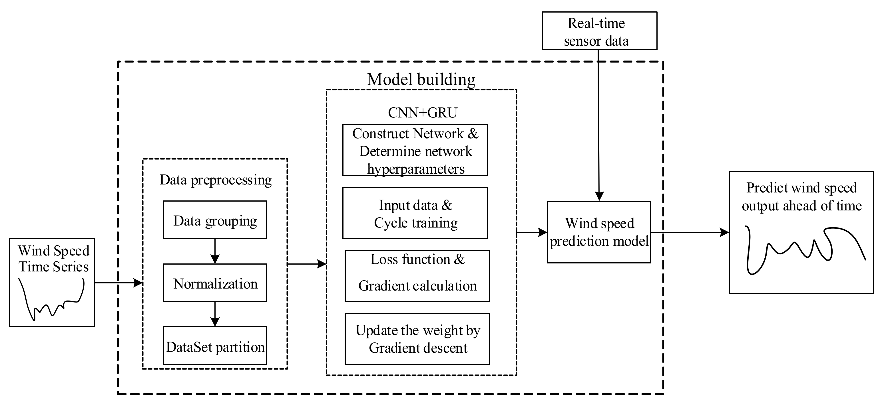
2.1. Full-Text Framework

The overall framework of this article is shown in Figure 1. It is divided into three modules: The data preprocessing module, model training module, and wind speed prediction module.

The data preprocessing module is mainly to distinguish the target domain data from the source domain data. The source domain data are used to train the model, while the target domain data are used to test the model. The model training module mainly constructs the network layer number and determines the hyperparameter of the network. The weight of the whole network is updated according to the minimum derivative of the loss function after cyclic training. The data used in this procedure is the source domain data. The wind speed prediction module is mainly to finetune a model obtained by training. Then the wind speed prediction of the target domain is realized by learning the target domain data. Of these three modules, the most important is the model training module. It is based on the CNN model and GRU network.

2.2. CNN Model

This paper adopts the basic convolutional neural network model, and the basic structure of the convolutional neural network is shown in Figure 2 below. A convolutional neural network can express the original data at a high and abstract level by the advantages of the convolution operation. It has an excellent performance in the image, signal waveform, and other fields [29]. Wind speed, air temperature, and other data are time-series data, which have local correlation, that is, data with similar times have a strong correlation. Therefore, using CNN to deal with its local features has a good effect.

The basic structure of CNN mainly includes a convolution layer and pooling layer. The convolution layer extracts data to the next layer by sliding the convolution kernel with a fixed size at a certain step. The pooling layer mainly deletes the similarity of data to reduce the computation of data. After the feature extraction of multiple convolution layers and pooling layers, the data is flattened and finally used as the output of the network through the full connection layer.

The convolution layer is constructed inspired by the biological research result that there is a receptive field when people observe things. The convolution operation is carried out by convolution with the appropriate size to check the information in the receptive field, by which the features of the original data are abstractly extracted. When the input data is $X$, the feature graph $C$ of the convolution layer can be expressed as follows:

$$C=f\left(X\otimes W+b\right)$$

(1)

where $\otimes$ is the convolution operation, $W$ is the weight vector of the convolution kernel, $b$ represents the offset, and $f\left(·\right)$ is the activation function. The activation function used in this article is the ReLu function. In this paper, 1-dim CNN is used to extract the features of the original data. 1-dim CNN can mine the correlation between multi-dimensional data and remove the noise and unstable components from it. The relatively stable information of the processed model is then transmitted to the GRU network as a whole for prediction.

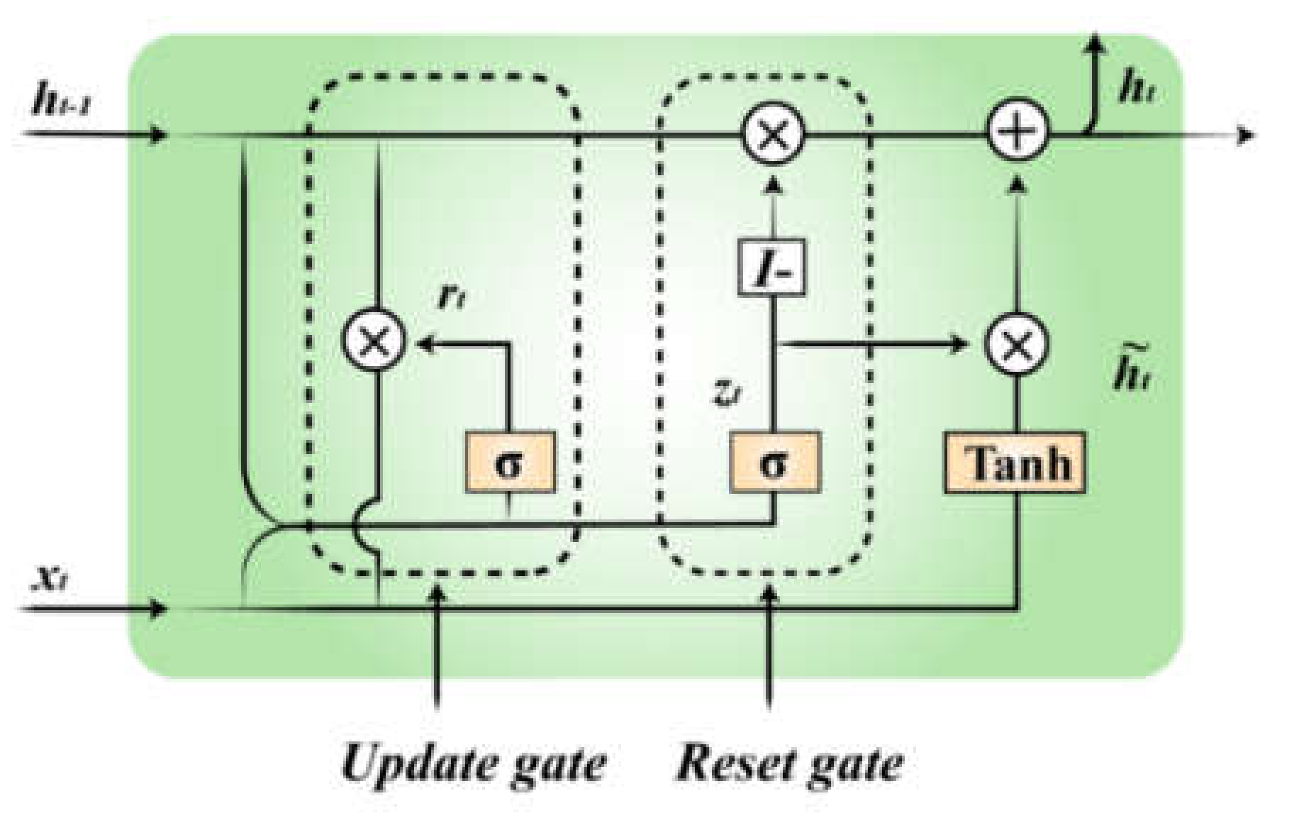
2.3. GRU Network

LSTM network is a recurrent neural network (RNN) architecture that can learn order dependency in nonlinear sequence prediction problems [30]. A Gated Recurrent Unit (GRU) network is an improved network model based on the optimization of the three gate functions of LSTM. The forgetting gate and input gate are integrated into a single update gate, and the neuron state and hidden state are mixed at the same time. GRU network can effectively alleviate the problem of “gradient disappearance” in the RNN network, reduce the number of parameters of the LSTM network unit, and shorten the training time [31]. The basic structure of the GRU network is shown in Figure 3, and the specific mathematical description is shown in Equation (2).

$$\left\{\begin{array}{l}{r}_t=\sigma \left(W_r·\left[h_{t-1},x_t\right]\right)\\ z_t=\sigma \left(W_z·\left[h_{t-1},x_t\right]\right)\\ {\tilde{h}}_t=\varphi \left(W_{\tilde{h}}·\left[r_t\times h_{t-1},x_t\right]\right)\\ h_t=\left(\mathrm{I}-z_t\right)\times h_{t-1}+z_t\times {\tilde{h}}_t\\ y_t=\sigma \left(W_o·h_t\right)\end{array}\right.$$

(2)

In Figure 3 and Equation (2), $x_t$, $h_{t-1}$, $h_t$, $r_t$, $z_t$, ${\tilde{h}}_t$, $y_t$ are the input vector, the state memory variable of the last moment, the state memory variable of the current moment, the state of the update gate, the state of the reset gate, the state of the current candidate set, and the output vector of the current time. $W_r$, $W_z$, $W_{\tilde{h}}$, $W_o$ are the weight parameters of the connection matrix multiplied by the update gate, reset gate and candidate set, and output vector, respectively. $\mathrm{I}$ represents the identity matrix. [ ] represents vector operations. $·$ represents the matrix dot product. $\times$ represents matrix products. $\sigma$ represents the sigmoid activation function. $\varphi$ represents the tanh activation function. The mathematical description of $\sigma$ and $\varphi$ is as follows:

$$\sigma \left(x\right)=\frac{1}{1+e^{-x}}$$

(3)

$$\varphi \left(x\right)=\frac{e^x-e^{-x}}{e^x+e^{-x}}$$

(4)

GRU has a recurrent and resetting of doors as its core module. The splicing matrix of the input variable $x_t$ and the state memory variable of the last moment $h_{t-1}$ is input into the update gate after sigmoid nonlinear transformation, which determines the extent of which the state variable is brought into the current state. Resets the amount of information that can be written to the candidate set at the last moment of the gate control. The information of the last moment is stored by $\mathrm{I}-z_t$ times $h_{t-1}$ and the information of the current moment is recorded by $z_t$ times ${\tilde{h}}_t$. These two are added together as the output of the current moment.

3. CNN—GRU Based on Transfer Learning

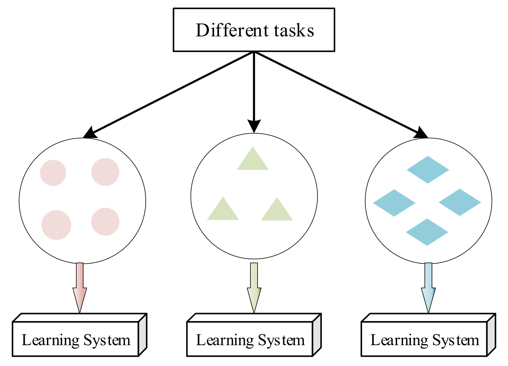
3.1. Transfer Learning

In traditional machine learning tasks, to ensure the accuracy and reliability of trained models, there are generally two assumptions: (1) The training samples and test samples are independent and identically distributed. (2) There must be enough training samples available to learn and get a good model. However, in practical application, these two conditions often cannot be met [32]. Transfer learning is a new machine learning method that uses existing knowledge to solve different but related fields and tasks. This approach relaxes two basic assumptions in traditional machine learning, whose purpose is to transfer the existing knowledge to solve the learning problem where there is only a small amount of labeled sample data in the target domain. The following figure shows how transfer learning differs from traditional machine learning processes.

As can be seen from Figure 4, deep learning requires a separate learning system for each task, and there is no connection between different systems. When constructing the system, different data are needed to train the learning system, which requires a lot of data and takes a lot of time. This method is not suitable for the less wind speed data and fast prediction speed at the initial stage of dam construction. Transfer learning is derived from deep learning. It can be seen from Figure 5 that, the features of source domain data are both independent and internal similar to those of target domain data, which are represented by color blocks. When solving the problem of the source domain, it is not necessary to build a new learning system from scratch but to apply the learning system of the source domain directly to the problem solving of the target domain after fine-tuning. Based on this idea, this paper uses transfer learning theory to predict wind speed in the complex terrain of dam construction, aiming at the difficulty of short-term wind speed data samples in the initial stage of the project.

The experimental purpose of this paper is to predict the wind speed during the construction of a hydropower station. Based on the above analysis, the requirement of wind speed prediction in dam construction is fast and accurate. So, we use one of the simplest transfer methods of a deep neural network—finetune. Finetune is an important technique in deep learning, which takes advantage of a trained network and adapts it to a specific task. Finetune is applicable if training and test data follow the same data distribution. In the data used in this paper, the source domain data is the meteorological data of the surrounding cities, and the target domain data is the meteorological data near the dam site. The data distribution of the two classes is the same, so the finetune method of transfer learning can be used.

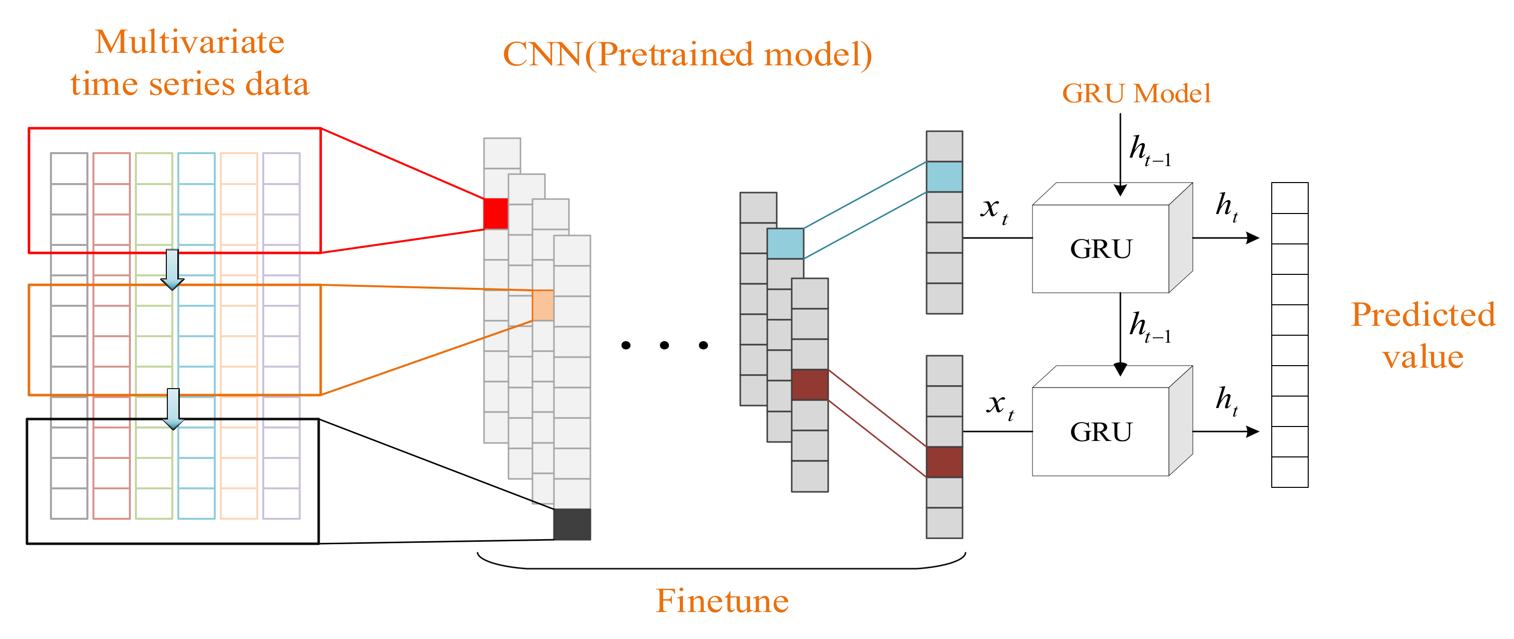
3.2. Hybrid Model of CNN—GRU Network Based on Transfer Learning

In this paper, the main architectures are a convolution neural network based on transfer learning and GRU. Firstly, temperature and wind speed data of existing stations were extracted by the CNN network combined with transfer learning to construct feature vectors of time series. Then the results are input into the GRU model for training, and the parameters in the network are updated and optimized by the optimization algorithm. The basic structure of CNN—GRU combined with transfer learning is shown in Figure 6 below.

In the mixed structure diagram of CNN—GRU, the data at the left is multivariate time series data, including wind speed data, air temperature data, humidity data, etc. These data are all-time series data, but the time series of wind speed is highly correlated. Therefore, these data are input into the CNN, and the convolution kernel extracts the original data layer-by-layer through the sliding window. The CNN not only extracts the independent features of each data but also extracts the correlation degree between different data. The middle part is the main structure of CNN and also the main fine-tuning part of transfer learning. The main body is trained by a large number of existing wind speed data, constantly optimizing the parameters of each layer, and then freezing the layer to save the best weight parameters for the subsequent wind speed prediction. The last module is the GRU model, which has been introduced in detail in the previous section. Its main function is to predict wind speed and finally output the predicted value of wind speed.

4. Results and Discussions

4.1. Experimental Data and Evaluation Indicators

The data set used in the experiment was taken from the real data of urban observation stations near the hydropower station. In this paper, hourly wind speed data after 25 May 2017, are selected. In the data set, each wind speed record includes six attributes: air temperature, wind direction, two-wind speed, two-wind direction, humidity, and pressure. Some wind speed records are shown in

Table 1. Partial meteorological data.

	Meteorological Data	Air Temperature (C°)	Wind Direction	Two-Wind Speed (m/s)	Two-Wind Direction	Humidity (%rh)	Pressure (pa)
Time
2017-05-25 12:00:00		23.8	341	4.6	348	45	941
2017-05-25 13:00:00		26.1	28	2.8	16	36	942
2017-05-25 14:00:00		27.0	355	6.2	347	34	942
2017-05-25 15:00:00		27.1	355	5.8	352	32	942
2017-05-25 16:00:00		27.3	341	6.3	339	32	944
2017-05-25 17:00:00		27.2	350	6.4	354	32	944
2017-05-25 18:00:00		27.0	350	6.2	358	32	944
2017-05-25 19:00:00		26.7	2	3.8	14	34	945
2017-05-25 20:00:00		24.5	94	1.2	137	53	942

. We use two different data for experiments in this paper. Data features of site one and site two are significantly different, as can be seen from observation values in Figure 7 and Figure 8. The fluctuation period of the wind speed data at site one is very short, which means that the wind speed data will fluctuate greatly in a very short interval. We use the data at site one to represent this kind of typical data. However, the fluctuation cycle of the data at site two is periodic, with fluctuations occurring every certain period. We use the data at site two to represent another type of periodic wind.

In this experiment, Mean Absolute Error (MAE) and Root Mean Square Error (RMSE) are taken for the performance evaluation. These two kinds of measurement indexes with their equations are shown in Equations (5) and (6).

$$\mathrm{MAE}=\frac{1}{N}{\displaystyle \sum _{n=1}^N\left|o_n-p_n\right|}$$

(5)

$$\mathrm{RMSE}=\sqrt{\frac{{\displaystyle \sum _{n=1}^N{\left(o_n-p_n\right)}^2}}{N}}$$

(6)

where $p_n$ denotes the predicted value, and $o_n$ represents the observed values. $N$ is the predicted length. The smaller MAE and RSME are, the closer the prediction is to the true value.

In this paper, some basic parameters of the training model are listed. Through repeated experiments, the aim is to minimize the loss function. There are some global settings that we used stochastic gradient descent (SGD) to train the proposed model and included an early stopping mechanism to prevent overfitting. Momentum was set to 0.5 and the learning rate $\eta$ was set to 0.001 in order to increase the speed of convergence, batch size set to 32, the dropout we set is different from the image processing, the setting is lower, which is 10%. The purpose of this is the high-level features of wind speed data are difficult to extract, the advantage is to keep the information features without adding redundant data. For a single convolutional layer, the size of the convolution kernel is $3\times 3$, the step size is one, and the padding is to fill zero at the edge. Finally, the number of GRU is one hundred. All experiments were conducted on a workstation running Keras as an interface for Tensorflow with an Intel Xeon Silver 4116 CPU, 64 GB RAM, and an Nvidia RTX 2080Ti GPU.

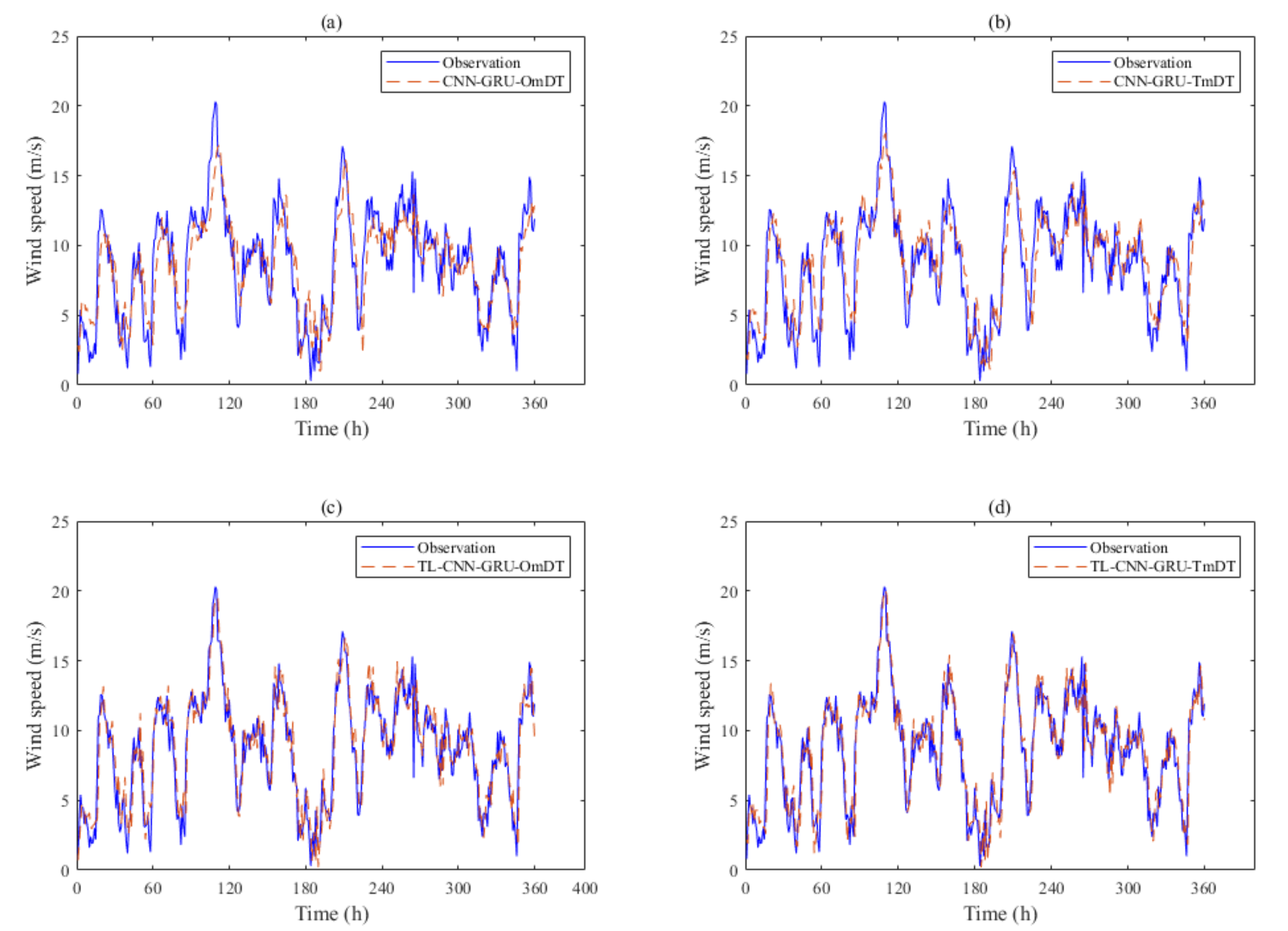
4.2. Discussion on Wind Speed Prediction at Site 1

The wind speed prediction of station 1 is discussed below. As mentioned above, the geographical location of station 1 belongs to Baihetan Hydropower, and the wind speed features have great fluctuation. We conduct experiments on the first 24-h data of wind speed data in the source region and carry out prediction experiments on the wind speed of this station by GRU model. Two ways of CNN combining with GRU model and CNN combining with GRU based on transfer learning are conducted. In this paper, a 15-day wind speed forecast is taken. The following Figure 7 shows the comparison of different experiment.

In Figure 7a,c use one-month data as the model obtained after training, while (c), (d) obtains the model after three-month training data. Figure 7a,b respectively show wind speed prediction based on CNN combined with GRU model. Figure 7c,d considered transfer learning. We can see from the figure that the model based on one-month wind speed data training is worse than based on three-month training data. The one-month training data models’ prediction deviation is higher than three-month training data models with large wind speed fluctuation, and the prediction value of these models does not overlap with the real value in the region with dense wind speed. This is because, in the case of a small number of wind speed samples, the pre-training of the model cannot extract wind speed characteristics well. It also can be seen that compared with the methods without transfer learning, the prediction bias of transfer learning models is significantly better. The two transfer learning models can predict both peak wind speed and time regions with dense wind speed well. Therefore, the method proposed in this paper has good predictability for the region with high wind speed fluctuation at site 1. The following

Table 2. Evaluation index accuracy of different model methods.

Train Data	GRU		CNN—GRU		TL—CNN—GRU
					Without Finetune		Only GRU Freezing		Training GRU with CNN Freezing
	MAE	RMSE	MAE	RMSE	MAE	RMSE	MAE	RMSE	MAE	RMSE
OmDT	1.832	2.325	1.704	2.162	1.437	1.853	1.334	1.740	1.235	1.701
TmDT	1.724	2.171	1.605	2.021	1.414	1.811	1.317	1.730	1.235	1.630

gives the evaluation indexes of different method models.

According to the above Table 2 and Figure 7, we can see that the disadvantage of using GRU alone is it has few parameters, but it cannot extract wind speed characteristics well. Therefore, the MAE and RMSE of this model are relatively high. Compared with the GRU model used alone, combining the CNN with the GRU model has improved prediction in the accuracy of wind speed. However, this model simply learns some basic wind speed characteristics from small sample data. It has poor learning ability for high peak wind speed and dense wind speed areas. Therefore, the accuracy of this model is still higher than the transfer learning model. The transfer learning model has three different ways discussed below:

(1)

The first way is directly use pre-training paraments without fine-tuning, and it has the worst prediction results. Whether it is small sample data or three months of sample data training, the results are higher than others. This is because if the model is not fine-tuned, the neural network will overfit the data set in the source domain, and the feature extraction of the data in the target domain is insufficient.

(2)

The second way uses a pre-training model with only GRU freezing. Compared with without fine-tuning model, this model has a better effect. By fine-tuning part of the neural network layer, the wind speed characteristics of the source domain data set can be fully obtained, and the over-fitting problem of the model can be further corrected by using the target domain data.

(3)

The third way trains GRU and CNN is frozen. This way performs best. It indicates that there are some differences in wind speed timing characteristics between the source region and target region. By taking the GRU layer as the fine-tuning network layer, we can not only learn the overall wind speed time series features in the source domain data, but also quickly obtain the wind speed time series features in the target domain, which effectively improves the feature extraction ability of the long wind speed series.

It can be concluded from the above analysis that the CNN combined with the GRU model based on training the GRU with the CNN freezing transfer learning is suitable for site 1, and it has the best prediction effect and the highest accuracy.

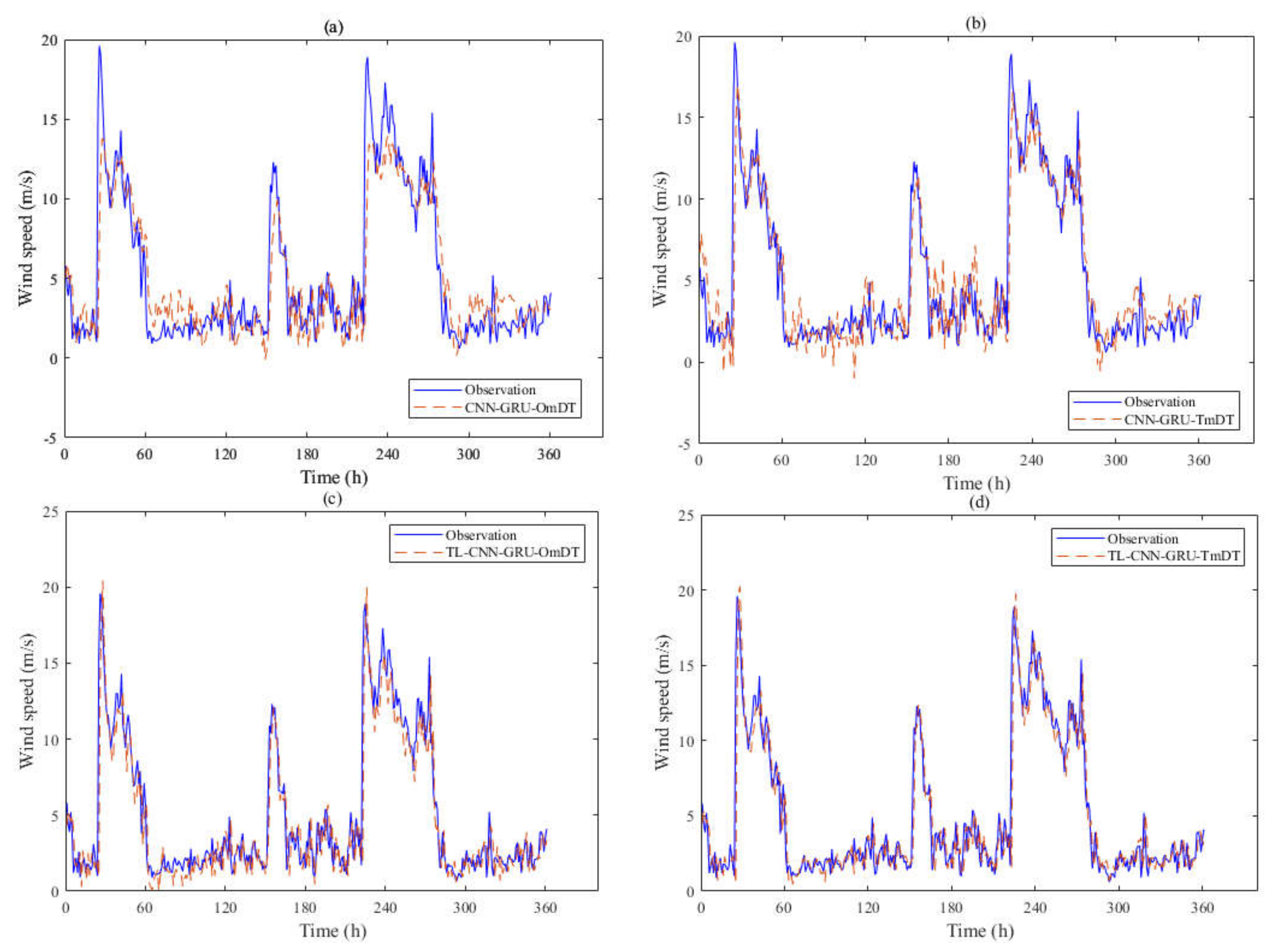
4.3. Discussion on Wind Speed Prediction at Station 2

Based on the above discussion of site 1, the selection of site 2 is geographically different from site 1. The selected test data of this site is smaller than the average value of the last site. Except for some extremely high peak moments, the fluctuation of wind speed of this site is relatively stable, and the average wind speed is lower than that of site 1, and the frequency of peak and wind speed peak is less. Therefore, the predicted overall evaluation index is better than that of site 1. The following Figure 8 shows the advantages and disadvantages of different models based on transfer learning.

Similar to the experimental content of site 1, Figure 8a,b is wind speed predictions based on the CNN combined with the GRU model. From this figure, we can see that the model of Figure 8a cannot predict the data well, either at the peak point of a wind speed or in the area with dense wind speed. This is due to the low long-term fluctuation of wind speed at site 2, with only a few days prone to strong winds. Therefore, it is more difficult to learn the wind speed characteristics of site 2, and it is difficult for CNN—GRU to learn the wind speed characteristics of this point by using the wind speed data of one month. Compared with Figure 8a, the wind speed prediction effect of Figure 8b is slightly better, but there is still a significant deviation from the real wind speed data. Figure 8c,d is CNN combined GRU models based on transfer learning respectively. It can be seen that the model can well predict the wind speed in the target region, even when the wind speed value is large. In practical engineering applications, the model has good performance. The following

Table 3. Evaluation index accuracy of different model methods.

Train Data	GRU		CNN—GRU		TL—CNN—GRU
					Without Finetune		Only GRU Freezing		Training GRU with CNN Freezing
	MAE	RMSE	MAE	RMSE	MAE	RMSE	MAE	RMSE	MAE	RMSE
OmDT	1.503	2.015	1.362	1.960	1.212	1.728	1.150	1.659	1.101	1.616
TmDT	1.363	1.920	1.288	1.836	1.143	1.656	1.089	1.612	1.039	1.569

gives the evaluation indexes of different models.

According to Table 3 and Figure 8, it can be found that the evaluation index of wind speed predicted by the GRU model alone is the worst. However, compared with site 1, the GRU model performed better at site 2, which has a certain reference value for areas with little fluctuation of wind speed. The effect of the CNN—GRU wind speed prediction and evaluation index is better than that of the GRU model alone because convolutional can better extract the wind speed characteristics of site 2 and improve the prediction ability of the network. The following is a discussion of transfer learning of this model in detail.

The first is horizontal analysis of the forecast for site 2. It can be seen from the table that the prediction effect of the model using one-month small sample data for training is close to that of using three-month data for training, which indicates that the model proposed in this paper still has a good effect in the initial stage of hydropower station construction when wind speed samples are insufficient.

Furthermore, the prediction accuracy of site 2 was compared longitudinally. As can be seen from the table, the prediction results of the model without fine-tuning are significantly higher than those of the model after fine-tuning, whether it is the small sample data or the sample with three months of sufficient data training. Since the wind speed characteristics of the two places are different, direct transfer learning without fine-tuning may lead to over-fitting of model parameters. Therefore, the weight parameters of the model need to be adjusted slightly to extract the wind speed characteristics of the two places. The structure of the GRU network determines that the GRU has fewer parameters, which reduces the problems caused by over-fitting. When training the GRU with freezing the CNN, it can achieve the best results among the three types of TL-CNN—GRU models, which indicates that although the data characteristics of the source domain and target domain are different, the data characteristics of the target domain can be quickly learned by using GRU. Therefore, the feature extraction ability of wind time series in the target region has been significantly improved.

This paper compares the proposed method with methods in other literatures, and the comparison results are shown in the

Table 4. Contrast between different methods.

Method	MAE	RMSE
Proposed method-site one	1.235	1.630
Proposed method-site two	1.039	1.569
RBF [33]	2.1525	2.1441
SHL-DNN [34]	1.6652	——
BP [35]	2.0199	2.0455

below:

As we can see from the table above, the proposed method in this paper has improved in different procedures compared with other methods in literature, especially for some traditional methods, the improvement is about 38%, which proves the excellence of TL-CNN—GRU, and this method has practical significance for the research of wind speed prediction.

5. Conclusions

This paper proposes a wind speed prediction model combining the CNN and GRU based on transfer learning, which is also suitable for the prediction of small sample wind speed data. We constructed a multi-layer convolutional neural network to extract wind speed characteristics, memorize past wind speed information through the GRU gating mechanism, and at the same time reduce the problem of gradient disappearance. First, a large number of wind speed data in the surrounding urban areas are used to pre-train the model, the purpose of this step is to get the hyperparameters of the model, the wind speed prediction model of hydropower station is obtained by fine-tuning, this step is the transfer learning method. The sharing model constructed by this method can effectively excavate the inherent and abstract sharing characteristics of wind speed in different fields. The experimental results show that the wind speed predicted by the proposed model is almost the same as the real data, within fifteen days of the real data, the wind speed fluctuation period at site one is short, and within a certain time interval, the wind speed fluctuation period at site two is long, which is completely different from the wind speed characteristics of site one. Experimental results show that the prediction results of these two kinds of data are very close to the actual values. The reason for this model’s good performance lies in that the CNN model is first used to extract high-level features of input data, and the GRU model is used to learn the relationship between time series, this model solves the difficulty of extracting high level features of wind speed data and the gradient disappearing when the model learns time series information. Through this method, the wind speed data can be fully mined. In summary, the model is effective for short-term wind speed prediction, which lays a foundation for the other short-term wind speed prediction.

References

- Yu, Q. China Southern Power Grid’s power supply reliability development strategy under digital transformation. J. Phys. Conf. Ser. 2021, 2005, 012030. [Google Scholar] [CrossRef]
- Sibtain, M.; Li, X.; Bashir, H.; Azam, M.I. Hydropower exploitation for Pakistan’s sustainable development: A SWOT analysis considering current situation, challenges, and prospects. Energy Strategy Rev. 2021, 38, 100728. [Google Scholar] [CrossRef]
- Kattelus, M.; Rahaman, M.M.; Varis, O. Hydropower development in Myanmar and its implications on regional energy cooperation. Int. J. Sustain. Soc. 2015, 7, 42–66. [Google Scholar] [CrossRef]
- Bekir, A. Estimation of Energy Produced in Hydroelectric Power Plant Industrial Automation Using Deep Learning and Hybrid Machine Learning Techniques. Electr. Power Compon. Syst. 2021, 49, 213–232. [Google Scholar]
- Catolico, A.C.C.; Maestrini, M.; Strauch, J.C.M.; Giusti, F.; Hunt, J. Socioeconomic impacts of large hydroelectric power plants in Brazil: A synthetic control assessment of Estreito hydropower plant. Renew. Sustain. Energy Rev. 2021, 151, 111508. [Google Scholar] [CrossRef]
- Zhao, Y.; Li, H.; Kubilay, A.; Carmeliet, J. Buoyancy effects on the flows around flat and steep street canyons in simplified urban settings subject to a neutral approaching boundary layer: Wind tunnel PIV measurements. Sci. Total Environ. 2021, 797, 149067. [Google Scholar] [CrossRef]
- Wang, L.; Chen, X.; Chen, H. Influencing Factors on Vehicles Lateral Stability on Tunnel Section in Mountainous Expressway under Strong Wind: A Case of Xi-Han Highway. Adv. Civ. Eng. 2020, 2020, 1983856. [Google Scholar] [CrossRef]
- Tropical Cyclone Gale Wind Radii Estimates for the Western North Pacific. 2018. Available online: https://www.researchgate.net/publication/314161314_Tropical_Cyclone_Gale_Wind_Radii_Estimates_for_the_Western_North_Pacific (accessed on 17 March 2022).
- Lei, M.; Shiyan, L.; Chuanwen, J.; Hongling, L.; Yan, Z. A review on the forecasting of wind speed and generated power. Renew. Sustain. Energy Rev. 2009, 13, 915–920. [Google Scholar] [CrossRef]
- Fouly, T.H.M.; Saadany, E.F.; Salama, M.M.A. One day ahead prediction of wind speed using annual trends. In Proceedings of the 2006 IEEE Power Engineering Society General Meeting, Montreal, QC, Canada, 18–22 June 2006; pp. 1–7. [Google Scholar]
- Landberg, L. Short-term prediction of the power production from wind farms. J. Wind. Eng. Ind. Aerodyn. 1999, 80, 207–220. [Google Scholar] [CrossRef]
- Liu, H.; Zhang, X.; Li, H.; Wang, Q. Wind speed forecasting in wind farm. Appl. Mech. Mater. 2014, 672, 672–674. [Google Scholar] [CrossRef]
- Negnevitsky, M.; Johnson, P.; Santoso, S. Short term wind power forecasting using hybrid intelligent systems. In Proceedings of the 2007 IEEE Power Engineering Society General Meeting, Tampa, FL, USA, 24–28 June 2007; pp. 1–4. [Google Scholar]
- Radziukynas, V.; Klementavicius, A. Short-term wind speed forecasting with ARIMA model. In Proceedings of the 2014 55th International Scientific Conference on Power and Electrical Engineering of Riga Technical University (RTUCON), Riga, Latvia, 14 October 2014. [Google Scholar]
- Kamal, L.; Jafri, Y.Z. Time series models to simulate and forecast hourly averaged wind speed in Quetta, Pakistan. Sol. Energy 1997, 61, 23–32. [Google Scholar] [CrossRef]
- Costa, A.; Crespo, A.; Navarro, J.; Lizcano, G.; Madsen, H.; Feitosa, E. A review on the young history of the wind power short-term prediction. Renew. Sustain. Energy Rev. 2008, 12, 1725–1744. [Google Scholar] [CrossRef] [Green Version]
- Onyelowe, K.C.; Mahesh, C.B.; Srikanth, B.; Nwa-David, C.; Obimba-Wogu, J.; Shakeri, J. Support vector machine (SVM) prediction of coefficients of curvature and uniformity of hybrid cement modified unsaturated soil with NQF inclusion. Clean. Eng. Technol. 2021, 5, 100290. [Google Scholar] [CrossRef]
- Barbounis, T.G.; Theocharis, J.B. A locally recurrent fuzzy neural network with application to the wind speed prediction using spatial correlation. Neurocomputing 2007, 70, 1525–1542. [Google Scholar] [CrossRef]
- Godarzi, A.A.; Amiri, R.M.; Talaei, A.; Jamasb, T. Predicting oil price movements: A dynamic Artificial Neural Network approach. Energy Policy 2014, 68, 371–382. [Google Scholar] [CrossRef] [Green Version]
- Mohandes, M.A.; Halawani, T.O.; Rehman, S.; Hussain, A.A. Support vector machines for wind speed prediction. Renew. Energy 2004, 29, 939–947. [Google Scholar] [CrossRef]
- Ji, G.R.; Han, P.; Zhai, Y.J. Wind speed forecasting based on support vector machine with forecasting error estimation. In Proceedings of the 2007 International Conference on Machine Learning and Cybernetics, Hong Kong, China, 19–22 August 2007; Volume 5, pp. 2735–2739. [Google Scholar]
- Salcedo-Sanz, S.; Ortiz-Garcı, E.G.; Pérez-Bellido, Á.M.; Portilla-Figueras, A.; Prieto, L. Short-term wind speed prediction based on evolutionary support vector regression algorithms. Expert Syst. Appl. 2011, 38, 4052–4057. [Google Scholar] [CrossRef]
- Zhou, J.; Shi, J.; Li, G. Fine tuning support vector machines for short-term wind speed forecasting. Energy Convers. Manag. 2011, 52, 1990–1998. [Google Scholar] [CrossRef]
- Hu, Q.; Zhang, S.; Xie, Z.; Mi, J.; Wan, J. Noise model-based v -support vector regression with its application to short-term wind speed forecasting. Neural Netw. 2014, 57, 1–11. [Google Scholar] [CrossRef]
- Alexiadis, M.C.; Dokopoulos, P.S.; Sahsamanoglou, H.S.; Manousaridis, I.M. Short-term forecasting of wind speed and related electrical power. Sol. Energy 1998, 63, 61–68. [Google Scholar] [CrossRef]
- Sideratos, G.; Hatziargyriou, N.D. An advanced statistical method for wind power forecasting. IEEE Trans. Power Syst. 2007, 22, 258–265. [Google Scholar] [CrossRef]
- Hafermann, L.; Becher, H.; Herrmann, C.; Klein, N.; Heinze, G.; Rauch, G. Statistical model building: Background “knowledge” based on inappropriate preselection causes misspecification. BMC Med. Res. Methodol. 2021, 21, 196. [Google Scholar] [CrossRef]
- Sun, Q.; Bourennane, S.; Liu, X. Multi-size and multi-model framework based on progressive growing and transfer learning for small target feature extraction and classification. Int. J. Remote Sens. 2021, 42, 8145–8164. [Google Scholar] [CrossRef]
- Gupta, L.; Edelen, A.; Neveu, N.; Mishra, A.; Mayes, C.; Kim, Y.K. Improving surrogate model accuracy for the LCLS-II injector frontend using convolutional neural networks and transfer learning. Mach. Learn. Sci. Technol. 2021, 2, 045025. [Google Scholar] [CrossRef]
- Karasu, S.; Altan, A. Crude oil time series prediction model based on LSTM network with chaotic Henry gas solubility optimization. Energy 2022, 242, 122964. [Google Scholar] [CrossRef]
- Saunders, A.; Drew, D.M.; Brink, W. Machine learning models perform better than traditional empirical models for stomatal conductance when applied to multiple tree species across different forest biomes. Trees For. People 2021, 6, 100139. [Google Scholar] [CrossRef]
- Mansour, R.F.; Escorcia-Gutierrez, J.; Gamarra, M.; Gupta, D.; Castillo, O.; Kumar, S. Unsupervised Deep Learning based Variational Autoencoder Model for COVID-19 Diagnosis and Classification. Pattern Recognit. Lett. 2021, 151, 267–274. [Google Scholar] [CrossRef]
- Zhang, Y.; Chen, B.; Pan, G. A novel hybrid model based on VMD-WT and PCA-BP-RBF neural network for short-term wind speed forecasting. Energy Convers. Manag. 2019, 195, 180–197, ISSN 0196-8904. [Google Scholar] [CrossRef]
- Hu, Q.; Zhang, R.; Zhou, Y. Transfer learning for short-term wind speed prediction with deep neural networks. Renew. Energy 2016, 85, 83–95. [Google Scholar] [CrossRef]
- Zhang, Y.; Wang, P.; Cheng, P.; Lei, S. Wind Speed Prediction with Wavelet Time Series Based on Lorenz Disturbance. Adv. Electr. Comput. Eng. 2017, 17, 107–114. [Google Scholar] [CrossRef]