Article

Projection of Extreme Temperature Events over the Mediterranean and Sahara Using Bias-Corrected CMIP6 Models

1
Binjiang College, Nanjing University of Information Science & Technology, Wuxi 214105, China
2
Wuxi Institute of Technology, Nanjing University of Information Science & Technology, Wuxi 214105, China
3
Jiangsu Key Laboratory of Atmospheric Environment Monitoring and Pollution Control, Collaborative Innovation Centre of Atmospheric Environment and Equipment Technology, School of Environmental Science and Engineering, Nanjing University of Information Science and Technology, Nanjing 210044, China
4
Organization of African Academic Doctors (OAAD), Off Kamiti Road, Nairobi P.O. Box 25305-00100, Kenya
5
Key Laboratory of Meteorological Disaster, Ministry of Education (KLME)/Joint International Research Laboratory of Climate and Environment Change (ILCEC)/Collaborative Innovation Center on Forecast and Evaluation of Meteorological Disasters (CIC-FEMD), Nanjing University of Information Science and Technology, Nanjing 210044, China
6
Research Institute for History of Science and Technology, Nanjing University of Information Science and Technology, Nanjing 210044, China
7
Department of Mathematics and Statistical Sciences, Botswana International University of Science and Technology, Private Bag 16, Palapye 10071, Botswana
8
International Water Research Institute, Mohammed VI Polytechnic University, Lot 660, Hay Moulay Rachid, Ben Guerir 43150, Morocco
*
Author to whom correspondence should be addressed.
Atmosphere 2022, 13(5), 741; https://doi.org/10.3390/atmos13050741
Submission received: 1 April 2022 / Revised: 26 April 2022 / Accepted: 5 May 2022 / Published: 6 May 2022
(This article belongs to the Section Climatology)

Abstract

:
Climate change continues to increase the intensity, frequency and impacts of weather and climate extremes. This work uses bias-adjusted Coupled Model Intercomparison Project Phase six (CMIP6) model datasets to investigate the future changes in temperature extremes over Mediterranean (MED) and Sahara (SAH) regions. The mid- (2041–2070) and far-future (2071–2100) are studied under two Shared Socioeconomic Pathways: SSP2-4.5 and SSP5-8.5 scenarios. Quantile mapping function greatly improved the performance of CMIP6 by reducing the notable biases to match the distribution of observation data, the Climate Prediction Center (CPC). Results show persistent significant warming throughout the 21st century, increasing with the increase in radiative forcing. The MED will record a higher increase in temperature extremes as compared to SAH. The warming is supported by the projected reduction in cold days (TX10p) and cold nights (TN10p), with the reduction in the number of cold nights exceeding cold days. Notably, warm spell duration index (WSDI) and summer days (SU) have a positive trend in both timelines over the entire study area. There is a need to simulate how climate sensitive sectors, such as water and agriculture, are likely to be affected by projected changes under different scenarios for informed decision making in the choice and implementation of adaptation and mitigation effective measures.

1. Introduction

Temperature change is of great interest in the backdrop of the ongoing anthropogenic global warming. Although mean change is being used to track the warming, emphasis has shifted to temperature extremes and its associated consequences. The impacts of temperature extremes are devastating, ranging from affecting both crop and animal productivity [1] to influencing evapotranspiration [2], as well as regulating human thermal comfort and health at large [3]. The impacts are highest in African countries that are highly vulnerable to climate variability and change effects due to over reliance on rainfed agriculture, limited resources and poor infrastructure [4].
The Mediterranean (MED) and Sahara (SAH) regions, as classified by the Intergovernmental Panel on Climate Change (IPCC) [5], remain climate change hotspots that require continuous monitoring. According to the report, on top of the observed and projected reduction in mean precipitation, the regions are likely to experience an increase in aridity and droughts. Further, the water-scarce regions are projected to record an increase in temperature that is likely to worsen the situation [6].
Although warming is a global phenomenon, Africa has been observed and is projected to warm at a higher rate than the global average, with North Africa ahead of other regions across the continent [2,5,7,8]. The observed climate change exhibits in the form of a warming trend characterized by longer and warmer summers, more frequent and severe heat waves, and a reduction in total rainfall, all of which are projected to persist throughout the 21st century [9,10,11,12,13,14]. Nangombe et al. [7] projected an increase in the frequency of hot days over North Africa as compared to other parts of the continent, attributed to the region’s fast increase in surface air temperature. The changes are likely to cause devastating impacts on water availability and quality, food quality, and air pollution, among others [15]. The observed changes are also expected to persist into the future over the Mediterranean [8,12,15,16,17,18]. In a study that extended to the Middle East, Zittis et al. [14] projected unprecedented super- and ultra-extreme heatwave conditions in the second half of the 21st century if only minimal or no efforts to limit greenhouse gas (GHG) emissions are put in place. This agrees with the conclusion of most studies, e.g., [7,15,19] have shown that efforts to limit warming to low levels are likely to be beneficial. This will help reduce both the intensity and frequency of extreme heat events not just across the north, but across Africa and, by extension, the Mediterranean.
Whilst the investigation of climatic change in the two regions is hindered by limited hydro-climatic datasets given that most of the region is arid to hyper arid, the growing availability of satellite and model datasets presents a solution to this challenge. The Coupled Model Intercomparison Project phase 6 (CMIP6) dataset is one of the latest datasets that gives both historical and projected changes in various weather parameters. This study is based on this dataset. Although the IPCC [5] is based on the data across the globe, Seneviratne and Hauser [20] pointed out the necessity of considering regional climate sensitivity as a discrete feature of Earth system models while studying regional climate changes.
These models are hindered by various uncertainties, mainly from emission scenarios, internal variability or/and model response uncertainty [21]. In order to improve the reliability of the model’s outputs, different spatial downscaling and bias correction algorithms (e.g., statistical and dynamic downscaling techniques) have been proposed and employed widely to reduce these inherent biases. Numerous studies, e.g., [22,23,24], have been conducted to determine the strength and weakness of various bias correction methods. Examples of such techniques include the delta correction [25,26], linear transformation [27], local intensity scaling [28], power transformation [29], distribution mapping [30,31], and quantile mapping bias correction [32,33]. Overall, these studies show that the quantile mapping algorithm depicts superior performance as compared to other approaches [34,35]. Several studies, e.g., [36,37], have thus employed quantile mapping methods and demonstrated the effectiveness of the approach in minimizing the biases in climate variables. For instance, Li et al. [38] established a remarkable improvement in the bias-adjusted temperature data.
To improve the accuracy of projections of temperature extremes, there is a need to first minimize the inherent biases before exploring the possible future changes in temperature over the diverse regions, such as MED and SAH. This study is the first of its kind to employ the bias corrected CMIP6 models in a bid to understand both spatial and temporal projected changes in extreme temperatures over MED and SAH under the various thermal forcing scenarios. This information is crucial in designing and implementing both adaptation and mitigation measures to combat climate change. The rest of the paper is formulated as follows: Section 2 highlights the climatological and geomorphological features of the study area, the datasets used and the methods employed, while Section 3 presents detailed results from a systematic analysis of the datasets herein. Lastly, Section 4 presents the key summary and conclusion of the present study.

2. Study Area, Data, and Methods
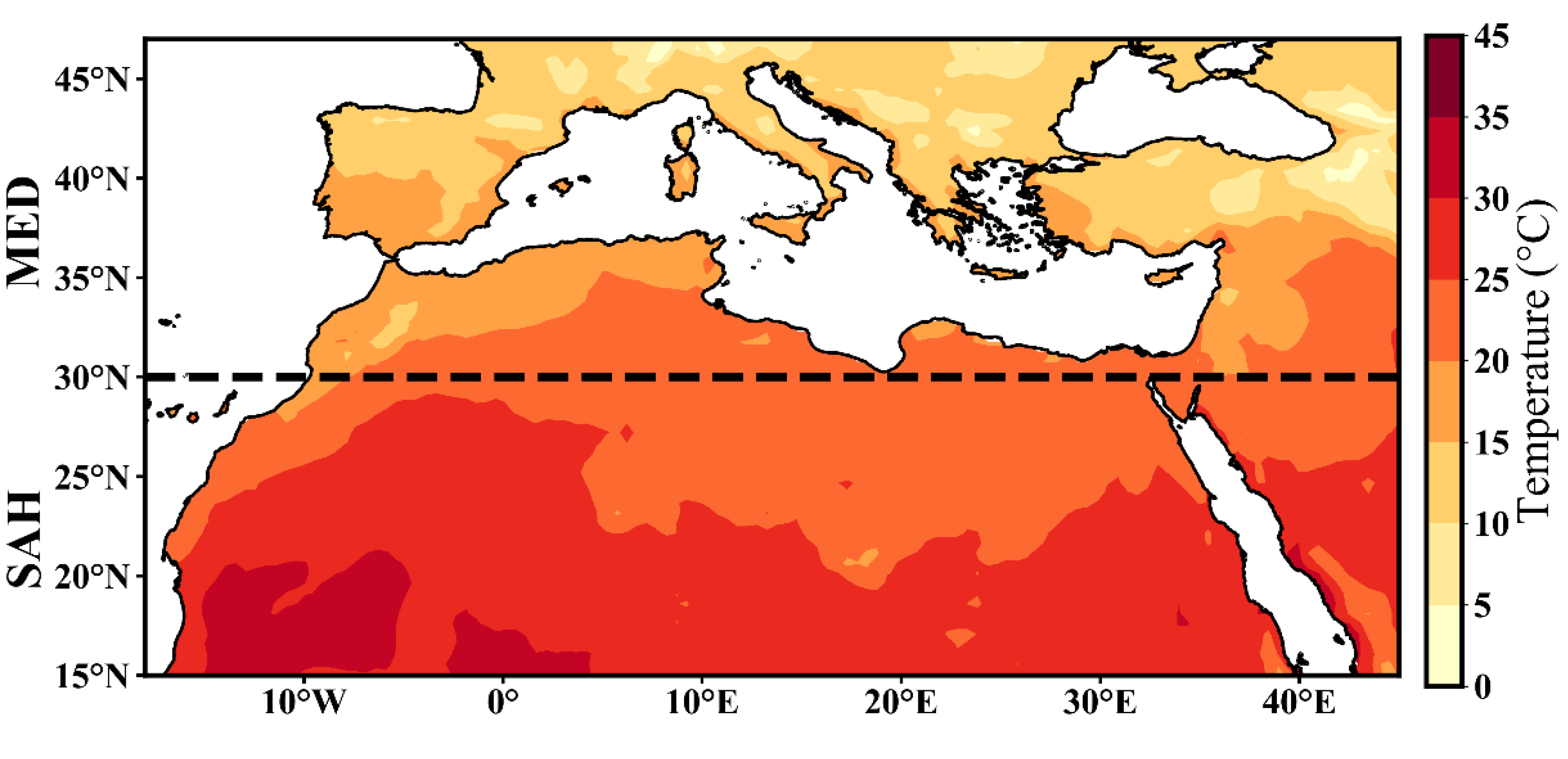
2.1. Study Area

The study domain (Figure 1) encompasses the southern region of Europe (Mediterranean) and the northern portion of Africa (Sahara). The domain is located between latitudes 14° N and 34° N, and longitudes 18° E and 45° E. The region has a complex topography, including the Atlas Mountains in the west, the Nile River in the east, and the Sahara Desert in the south. The climate in the region varies greatly between the coast and the inland regions, as well as from north to south [39,40]. The northern portion along the Mediterranean Sea has a Mediterranean climate, which is characterized by a hot, dry summer and a cold, wet winter. During summer, the average temperature is around 22 °C, while in winter it ranges between 18 °C and −3 °C. The mountains surrounding the region influence rainfall and temperature distribution over the region. In the southern portion of the study domain, the climate is semiarid to arid (desert) [41]. During winter, the average temperature over the region is around 24 °C. In the summer season, which can stretch from 2–5 months, the average temperature is 35 °C, but can reach up to 45 °C. The latest IPCC climate reference [42] classifies the region into two sub-regions, the Mediterranean (MED) and Sahara (SAH), as shown in Figure 1.

2.2. Data

2.2.1. Observations

The gauge-based gridded temperature dataset employed in this study is obtained from the Climate Prediction Center (CPC) of the National Oceanic and Atmospheric Administration (NOAA). The data has a horizontal resolution of 0.5° × 0.5°, running from 1979 to date. The CPC dataset is preferred over other surface air temperature datasets because it combines two large individual datasets of station observations sourced from the Global Historical Climatology Network version 2 and the Climate Anomaly Monitoring System (GHCN + CAMS) provided by NOAA, Boulder, Colorado, USA. This allows it to be updated in near real-time with a large number of stations [43]. A number of studies, e.g., [5,44], have used the CPC over the study domain, thereby reaffirming its reliability.

2.2.2. Model Datasets

This study utilizes multi-model mean ensemble (hereafter MME) of historical and projected surface air temperature datasets from 23 CMIP6 models [45]. The datasets cover two time periods: 1850–2014 and 2015–2100 for historical and future periods, respectively. The comparison analysis is conducted in two equal time slices: mid-century (2041–2070) and far-future (2071–2100) relative to the baseline period (1995–2014), recommended by the sixth assessment report of the IPCC (AR6). The shared socioeconomic pathway scenarios (SSP): SSP2-4.5 and SSP5-8.5 that represent modest mitigation and worst-case scenarios are employed in the study. The SSP2-4.5 scenario is regarded as a more realistic emission scenario, with moderate mitigation efforts limiting global warming to 2.5 °C above pre-industrial levels by the end of the 21st century [46]. The SSP5-8.5 with the strong forcing scenario (commonly known as “business as usual”), on the other hand, predicts a fossil-fuel-intensive future devoid of strict climate mitigation, resulting in approximately 5 °C of warming by the end of the century. The two radiative forcing scenarios were chosen from among the five potential frameworks on the assumption that changes in climate outcomes between scenarios for the global pathways are expected to be minimal in contrast to changing regional climate characteristics [43,46]. The first realization ensemble (r1i1p1f1) is considered in the study to allow equal and comparable analysis. Table 1 shows the models employed in the study, their developing institutions, and native resolutions.

2.3. Methods

2.3.1. Computation of Temperature Extremes Indices

The present study employs ten temperature extreme indices defined by the Expert Team on Climate Change and Detection Indices (ETCCDI [47]) to explore the projected changes in temperature extremes over the MED and SAH, a region that is classified as a climate change hotspot [6]. The indices are selected to examine the changes in temperature intensity (hottest day, warmest night, coldest day, coldest night), duration (warm spell duration and summer days), and frequency (warm days, warm nights, cold days, and cold nights) over the study region. The robustness of the indices has been affirmed based on their applicability by numerous studies across various regions [48,49,50,51]. Details on the indices is provided in Table 2. The ten extreme temperature indices (hereafter referred to as indices) are computed for the observations and all the 23 CMIP6 General circulation models (GCMs) historical and projection data. For uniformity in models and observations horizontal resolutions, all datasets were regridded to a 1° × 1° spatial resolution using a bilinear interpolation technique. This process aids in increasing spatial resolution, and thus improves the model performance in capturing the geomorphological features of the land that influence temperature variation.

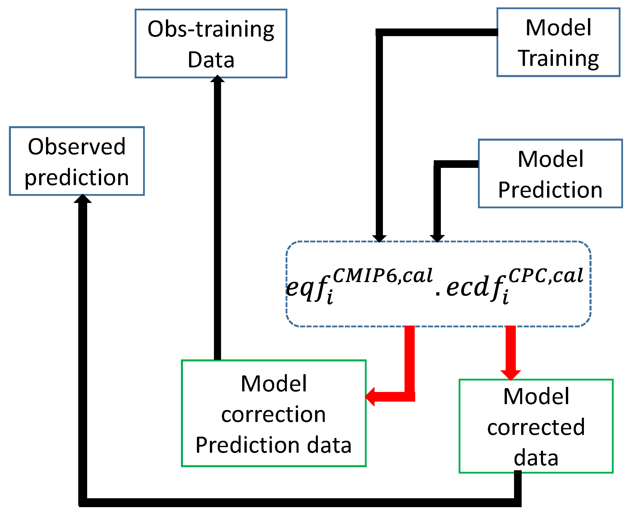
2.3.2. Bias Correction Method

This study uses the quantile mapping approach for bias correction. The quantile mapping matches the Cumulative distribution function (CDF) of the model distribution to that of the observation, and adjusts the frequency and intensity of the daily modelled temperature data [32]. The quantile mapping equation for temperature is shown in Equation (1);
QM i = x i + F o - 1 ( F ms ( x i ) )   -   F mh - 1 ( F ms ( x i ) )  
where QMi is the bias-adjusted data for the quantile mapping at point i, F represents the CDF, and F−1 is its inverse. o is the observation, mh is the model in the historical period, and ms is the model simulation (the simulation period is for either a historical or a projection time scale). xi is the data point in the CDF distribution. The bias adjustment is applied using the Climate Data Bias Corrector [52]. The quantile mapping is conducted on each grid of the model data, and the resulting data is used to compute the temperature indices introduced in Section 2.3.1.

Testing the Reliability of the Model Correction Approach

Whereas there are many approaches for testing the reliability of the model correction method, this study employed the split sample testing (SST) to assess the effectiveness of quantile mapping technique. More information about the SST approach is detailed by Klemeš [53]. To illustrate, SST approach involves separating datasets into two segments, where one is used for training, and another is utilized for validation. In this study, the first 16 years (1979–1994) were used for training by deriving the biases field for monthly averages in the model and observed temperature simulations. The monthly biased field was then utilized to adjust the independent GCMs during the validation period of 1995–2014. Moreover, the projection estimates under SSPs 2-4.5 and SSP5-8.5 were then corrected during the periods investigated (i.e., 2041–2070 and 2071–2100). Figure 2 presents a flowchart of the SST approach applied herein.
The flowchart (Figure 2) shows the testing for reliability of the quantile bias correction approach with two input data sources for observation and model simulations that are inputted for the transform function in Equation (1). The functions of ( e q f i c m i p 6 ,   c a l . c d f i c p c , c a l )   ( C M I P 6 t , i v a l ) , e d f shows empirical quantile function; the inverse of the CDF and the operator (°) denotes the function’s content. The C M I P 6   a n d   C P C refer to the GCMs simulations and observed temperature products, respectively. The superscript c a l refers to calibration, while the superscript v a l refers to validation. The output, which is model corrected, is then used for the validation process. For instance, the model for future correction uses three input files for bias corrections (i.e., observed historical data, model simulated historical data, and the model scenarios for future data). The effectiveness of the approach is tested using empirical cumulative distribution function (ECDF) where models before and after are presented to show the reduction of biases in temperature datasets to be used for the examination of extreme events.

2.3.3. Future Changes in Temperature Extremes

Changes in temperature projections are analyzed under SSP2-4.5 and SSP5-8.5 scenarios in two timescales: mid-future (2041–2070) and far-future (2071–2100) relative to the baseline period (1995–2014). Projected changes are computed on bias-adjusted MME. The study employed MME as a way of reducing uncertainties and ensure more reliable projections [54]. The underlying assumptions of the MME are that all models are reasonably independent, equally plausible, and distributed around the reality [55]. Further, Modified Mann–Kendall [56] was employed to determine the changes in extreme temperature trends over the MED and SAH regions, while the shift in distribution is examined using the box-and-whisker technique. This method is useful in graphically comparing various temperature characteristics. It highlights the distribution of datasets based on five key indicators: minimum value, first quartile (25th percentile), median, third quartile (75th percentile) and maximum value. The interquartile range shows the changes in temperature events. This approach has been utilized in various studies (e.g., [57,58,59]).

3. Results

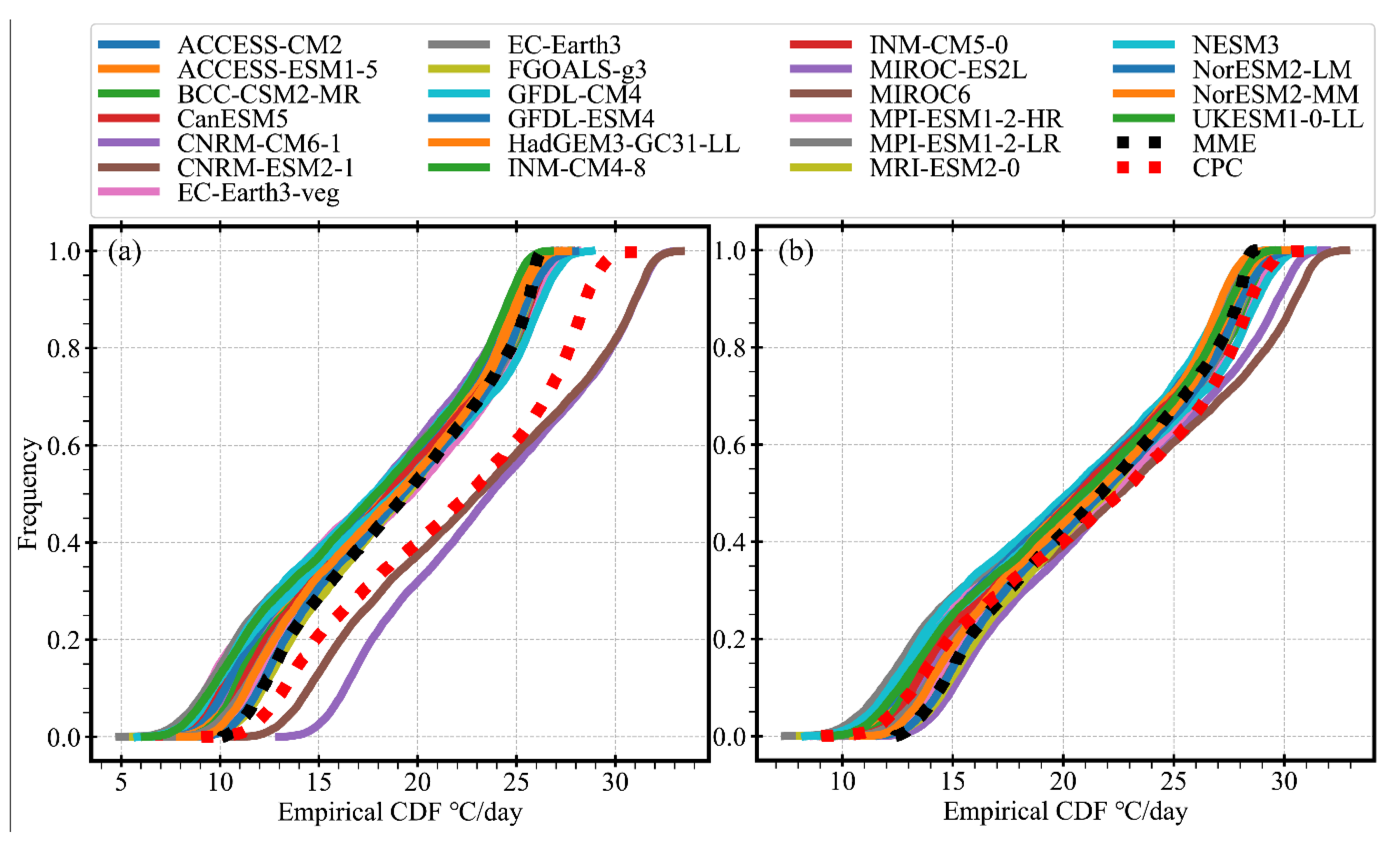
3.1. Bias Adjustment of Daily Temperature

The results obtained from a pixel-wise quantile mapping bias correction analysis are shown in Figure 3. Figure 3a shows the distribution of individual models and their respective mean ensemble against the observation using the empirical cumulative density function (ECDF) before correction. The bias corrected CMIP6 models using CPC as constraint over the study region during 1995–2014 is given in Figure 3b. It is evident from the analyses that quantile mapping function greatly improved the performance of CMIP6 by reducing the notable biases to match the distribution of observation data. The GCMs before correction show that about 90% of temperature datasets depict cold biases, while 10% (i.e., MIROC-ES2L and MIROC6) show large warm biases of >15 °C (Figure 3a). However, upon correction, all models including the mean ensemble demonstrate satisfactory distribution similar to the observation, thus reaffirming the effectiveness of technique prior to conducting impact analyses. The hypothesis that the distribution during the observational period will remain in the future is adopted following the recommendation by previous studies, e.g., [60,61]. Consequently, we also assume the stationarity of climate in conducting the bias correction for projection data and computing the climate indices. The present findings agree with existing studies that highly recommend the correction of inherent GCM biases before employing the data for impact studies [37,62,63]. In fact, recent studies that employed GCMs in projecting extreme events, such as high temperatures and extreme precipitation, equally conducted bias correction before using the models in examining the projected changes over various locales [49,63,64].

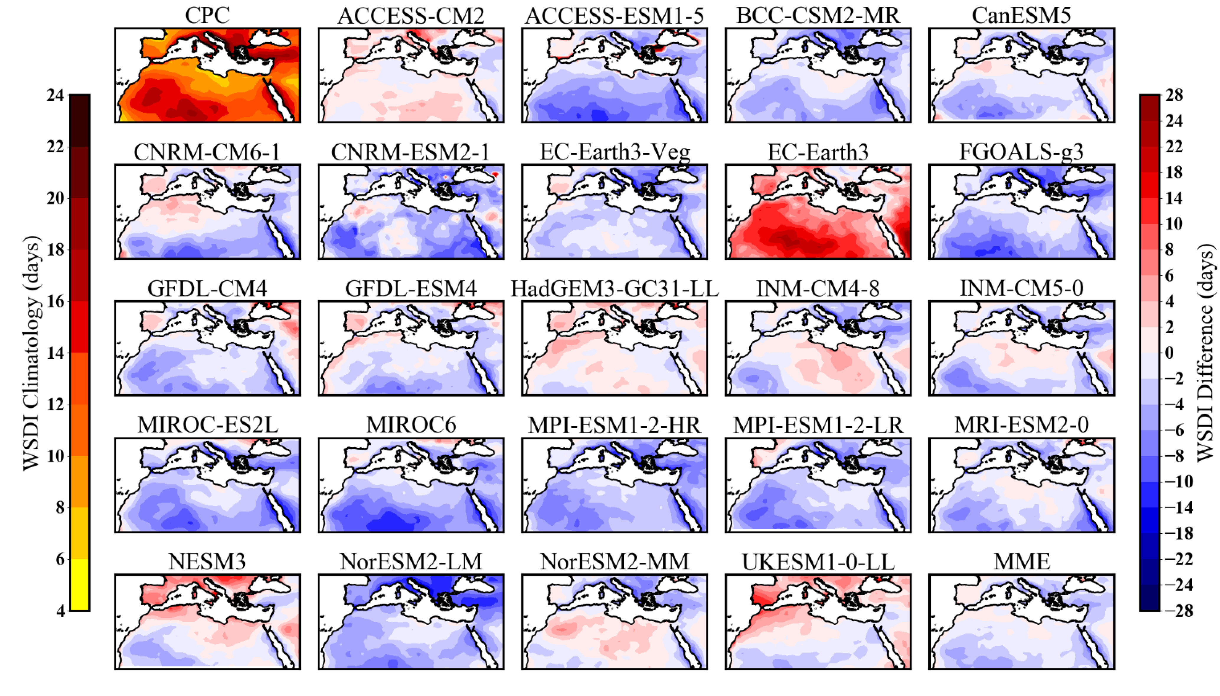
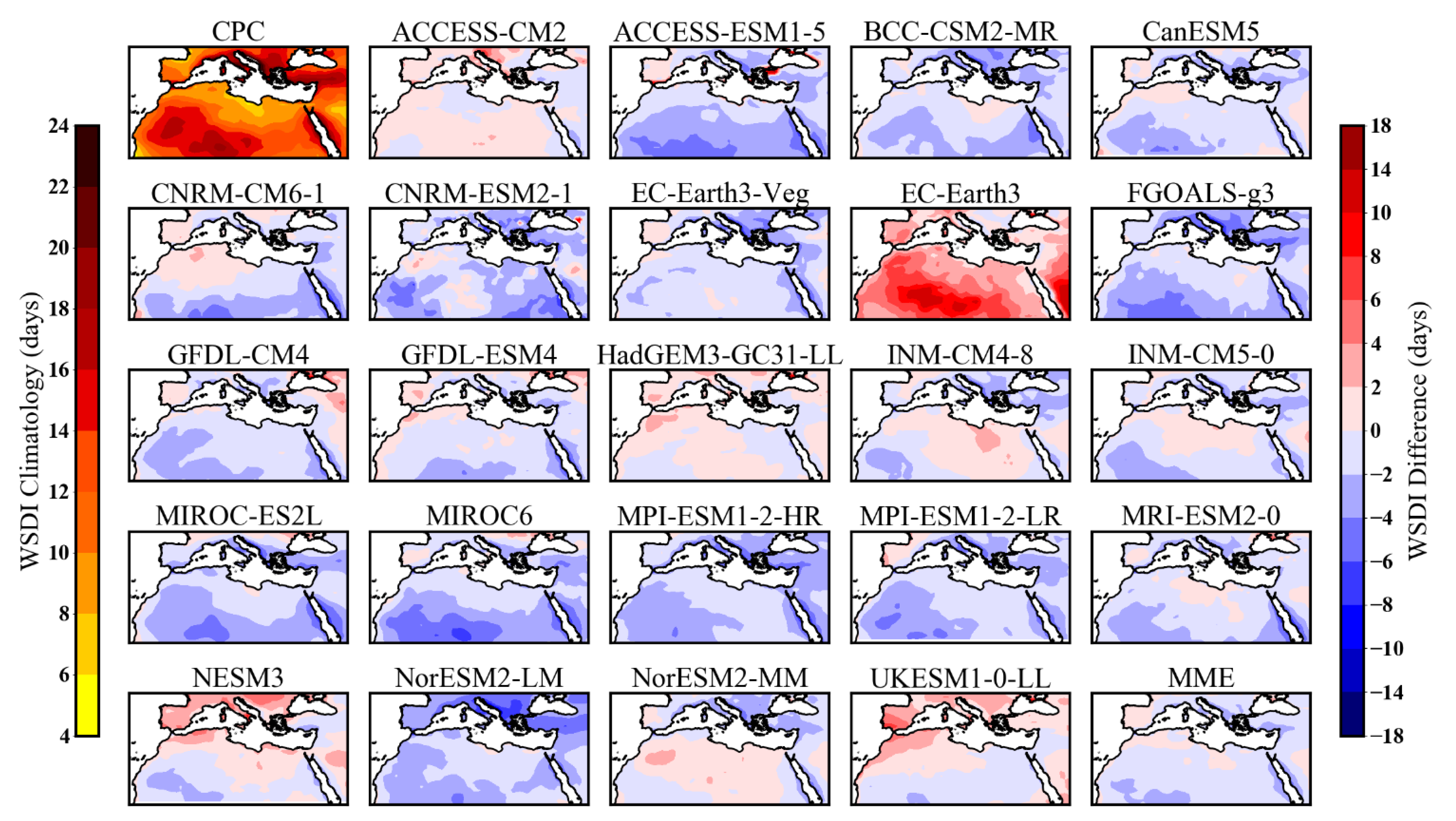
3.2. Magnitude of Absolute Error in Bias Correction Estimates for Temperature Extremes

The spatial bias before and after correction for individual models and their MME for all indices are equally evaluated against the observation over the study domain. Due to the large number of indices and models employed, we only present the anomalies of warm spell duration index (WSDI) as a representative of the analysis (Figure 4 and Figure 5); the rest of the indices and models are presented as Supplementary Materials (Figures S1–S18). Observational data shows the occurrence of WSDI over most of the MED region with values up to 24 days, while the SAH parts show WSDI of 8–15 days. The results show cold bias (less WSDI), except for a few models such as EC-Earth3, UKESM1-0LL, and ACCESS-CM2 (Figure 4). Remarkably, most models demonstrate excellent reduction in biases with the differences reduced from 28 days (before) to 18 days (after correction) (Figure 5). Models showing cold/warm biases in some parts of the study domain are corrected to match the observations. Similar improvement is noted in other indices as presented in the Supplementary Materials. Overall, these results suggest that quantile mapping function improves the capability of individual models in simulating the observed temperature extremes. A similar approach was employed in a study that utilized the CORDEX-Africa regional climate models (i.e., [63]), with results demonstrating satisfactory performance of the models in depicting temperature extremes. The study noted that when biases are accounted for, projected risks of extreme temperature-related hazards are higher than in non-bias-adjusted models. This shows that the GCMs and RCMs models that have been further improved using statistical or dynamical algorithms have a strong capability to simulate the observed changes in temperature properties across various regions. Consequently, our study employed bias-corrected GCMs of CMIP6 model outputs to explore the possible future changes in temperature extremes over MED and SAH region during the mid- and far-future period.

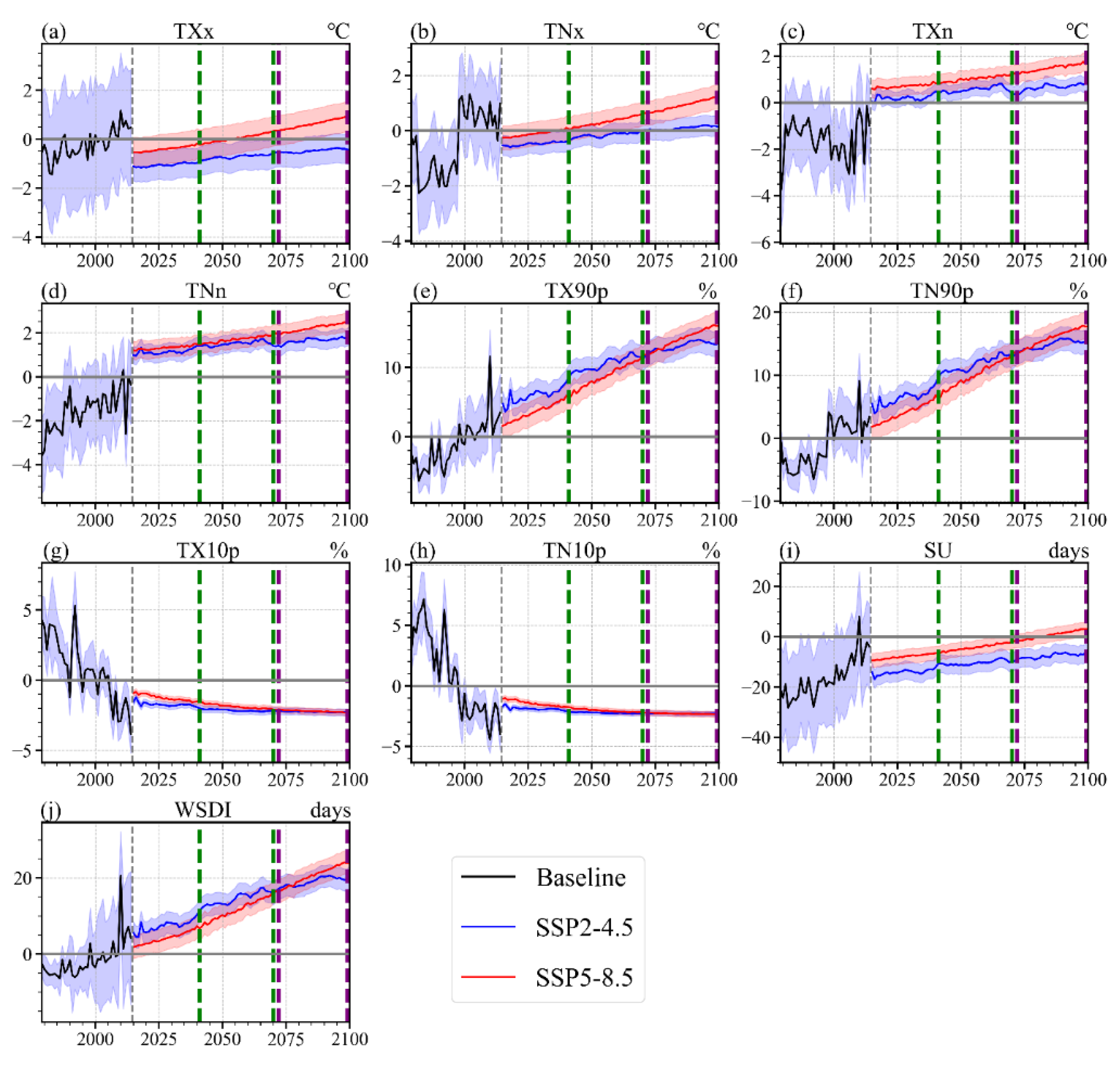
3.3. Temperature Projections for the 21st Century

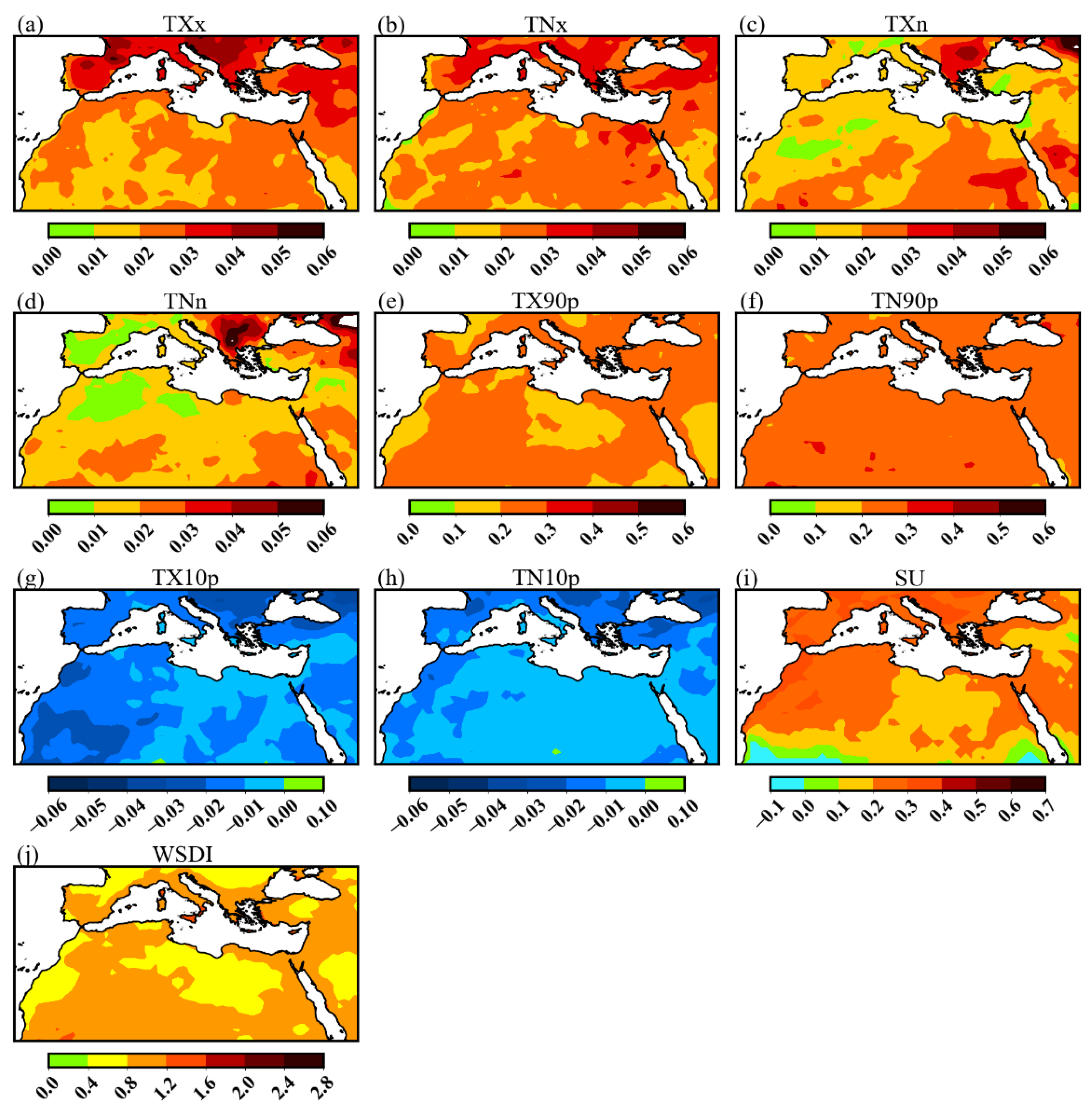
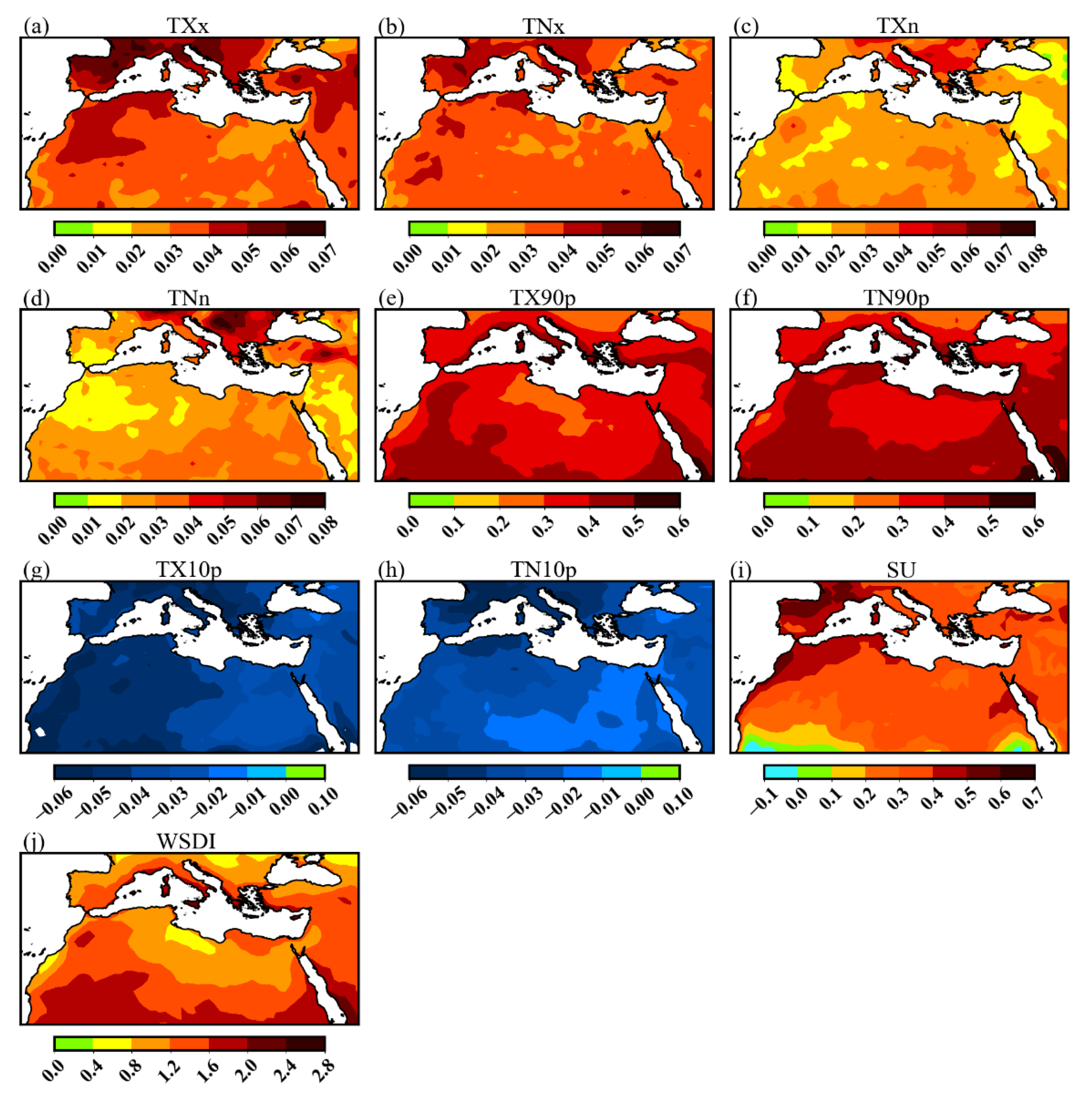
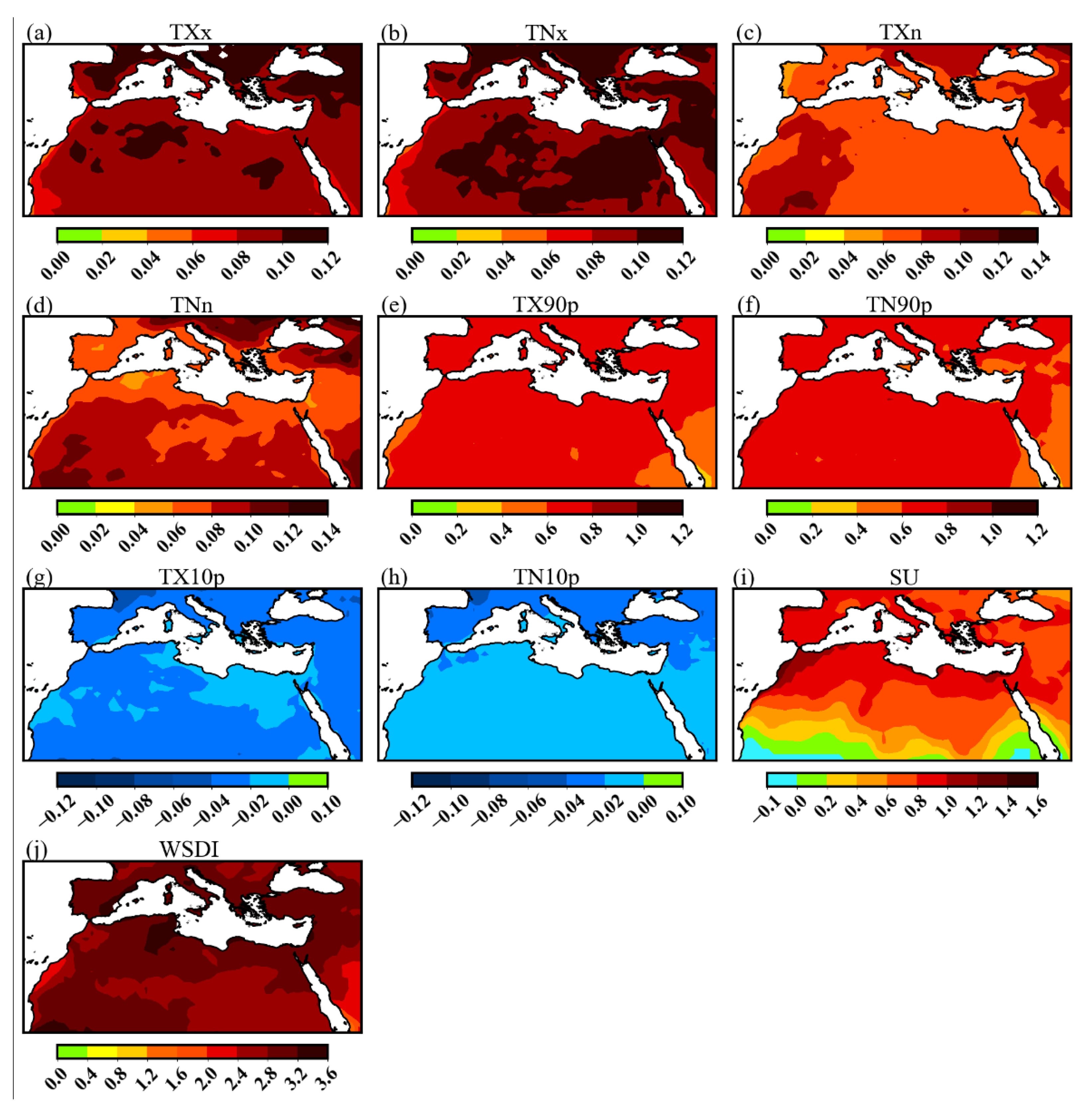
3.3.1. Projected Changes in Spatial and Temporal Anomalies

Projected changes of various temperature extremes under the SSP2-4.5 and SSP5-8.5 scenarios during the mid-future of 2041–2070 and the far-future (2071–2100) are computed from the mean multi-model ensemble of CMIP6. Figure 6 and Figure 7 show spatial changes in temperature extremes based on CMIP6-MME under the SSP2-4.5 scenario. Correspondingly, SSP5-8.5 scenario changes are presented in Figure 8 and Figure 9. Lastly, temporal analysis is presented in Figure 10. In agreement with existing studies evident from previous model simulations derived from CMIP5 [65], and a recent global study based on the CMIP6 dataset [66], temperature extremes project continued warming across the study region.
The annual maximum temperature (TXx) over the region exhibits pronounced warming towards the end of the century as compared to mid-century in both scenarios. The MED is projected to warm more than the SAH region. For example, the MED location will experience an increase in TXx of 2 °C to 4 °C during the mid-future under the SSP2-4.5 scenario, whereas the SAH domain will record an increase of TXx at 1 °C to 2 °C relative to the baseline period (Figure 6a and Figure 10a). Changes projected to the end of the century under the same scenario show an increase in TXx over SAH of 2 °C to 3 °C, while MED warms by 3 °C to 5 °C (Figure 7a and Figure 10a). Obviously, under the SSP5-8.5 scenario, a significant upsurge in TXx during mid-century is projected over SAH at 2 °C to 3 °C and MED at 4 °C to 8 °C compared to 1995–2014 TXx values (Figure 8a and Figure 10a). It is evident that the region will experience stronger warming towards the end of the century relative to the baseline period, with expected TXx projected to be at 4 °C to 6 °C over SAH and 6 °C to 10 °C over MED (Figure 9a and Figure 10a). Generally, scenario comparison reveals substantial warming under the SSP5-8.5 scenario as compared to the SSP2-4.5 scenario. Moreover, towards the end of the century, the TXx will be most likely to affect the MED region as compared to the SAH region.
Considering the changes in the annual maximum value of the daily minimum temperature (TNx) under different scenarios and timescales, these also show distinct changes. Under the SSP2-4.5 scenario, a notable increase in TNx is projected to occur over the MED by 1 °C to 3 °C as compared to SAH, which will experience slight changes at −2 °C to 0 °C in most parts during mid-century (Figure 6b and Figure 10b). However, in the far-future, a persistent higher increase in the warmest nights is projected to occur over MED at 2 °C to 5 °C compared to SAH at 0 °C to 2 °C (Figure 7b and Figure 10b). Interestingly, some regions in SAH, such as areas covering Libya and Mauritania, will experience less changes in TNx during the mid- and far-future relative to the baseline period (Figure 6b, Figure 7b and Figure 10b). Analysis of projected changes under a high emission scenario during the 2041–2070 period compared to 1995–2014 shows similar patterns in SSP2-4.5, but with a more intense increase in TNx at 3 °C to 6 °C (Figure 8b and Figure 10b). The changes will further surge towards the end of the century, increasing from 6 °C to 10 °C (Figure 9b and Figure 10b). Eventually, future changes over SAH show uniform warming during the far-future with an increase in TNx of 2 °C to 4 °C (Figure 9b and Figure 10b) as compared to mid-century, at a 1 °C to 2 °C increment relative to the historical period (Figure 8b and Figure 10b).
The changes in the annual minimum value of daily maximum temperature (TXn) and the annual minimum value of daily minimum temperature (TNn) demonstrate a diverse variation during the mid- and far-future under SSP2-4.5. However, uniform changes are projected under the SSP5-8.5 scenario for both timelines under consideration. For example, under SSP2-4.5, most parts of the MED region will record an increase in TXn and TNn during the mid-century at 1 °C to 3 °C, while over SAH, only southern parts will experience an increase in TXn at 1 °C to 3 °C (Figure 6c,d and Figure 10c,d). Similar changes are noted during the far-future for TXn, although a slight increase is projected for TNn over SAH at 1 °C to 2 °C and for MED at 1 °C to 3 °C (Figure 7c,d and Figure 10c,d). Meanwhile, changes in TXn and TNn under the SSP5-8.5 scenario show robust changes both for the mid-future and far-future, respectively (Figure 8c,d, Figure 9c,d and Figure 10c,d). For instance, during the 2041–2070 period, TXn is expected to increase by 2 °C to 4 °C over SAH and 1 °C to 3 °C over MED, whereas TNn is expected to increase by 2 °C to 7 °C over MED and 2 °C to 4 °C over SAH (Figure 8c,d). Robust and intense TNn changes are projected towards the end of the century over MED at 3 °C to 9 °C, and 4 °C to 6 °C over SAH (Figure 9d and Figure 10d).
In general, projected changes in temperature extremes over MED and SAH agree with previous studies that were based on CMIP5 or RCMs over the same study domain [44,67,68,69,70,71]. The evidence from the aforementioned studies indicated an increase in the intensity and frequency of hot extremes and a decrease in cold extremes. Likewise, the present study projects the highest increase in temperature extremes towards the end of the century under a high emission scenario as compared to mid-century or under a modest mitigation scenario. In fact, the projected changes in the warmest nights (TN90p; Figure 9f and Figure 10f) will be higher than the warming in the warmest days (TX90p; Figure 9e and Figure 10e). Conversely, a sharp decline in cold days (TX10p; Figure 9g and Figure 10g) and cold nights (TN10p; Figure 9h and Figure 10h) is projected to occur during the mid-century and far-future in both the SSP2-4.5 and SSP5-8.5 scenarios. Simultaneously, the duration indices (SU and WSDI; Figure 9i,j and Figure 10i,j) equally show robust changes over MED as compared to SAH during 2041–2070 and 2071–2100 under the SSP5-8.5 scenario. This shows that the region will be a climate change hotspot with areas that were previously cooler warming up. This will expose the population, ecosystem, and built infrastructure to excessive heatwaves and thermal discomfort.

3.3.2. Projected Trends

Figure 11, Figure 12, Figure 13 and Figure 14 show annual spatial trends temperature indices for the periods 2041 to 2070 and 2071–2100 compared to the baseline (1995–2014). The analyses are based on the CMIP6-MME under the SSP2-4.5 and SSP5-8.5 scenarios. A summary of statistical trends analysis indices is presented in Table 3. It is evident that the region will experience statistically significant increasing trends in TXx, TNx, TX90p, TN90p, SU and WSDI in both timelines and scenarios (Table 3). On the other hand, TXn and TNn depict insignificant increasing trends during the mid- (0.01–0.06/year) and far-future (0.01–0.08/year) under the SSP2-4.5 scenario (Figure 11c,d and Figure 12c,d). Interestingly, TNx is most pronounced in areas over Egypt, the southern section of Libya and Algeria at a (Z = 3.25) significant level during the far-future under the SSP5-8.5 scenario (Figure 14b, Table 3). Conversely, TX10p and TN10p reveal significant decreasing trends (−0.01 to −0.12/year) over the study region in both timescales and scenarios under consideration (Figure 11g,h, Figure 12g,h and Figure 13g,h). Spatial trends for TXx and TNx depict robust changes over MED under the SSP2-4.5 scenario during the mid-future with a positive significant trend (Z = 3.39) and far-future (Z = 3.18), while uniform positive trends are experienced under the high emission scenario during the two time periods (Figure 13a,b and Figure 12a,b). Projected trends in warmest days (TX90p) and warmest nights (TN90p) across the entire domain during the mid- and far-future timescales depict strong significant positive trends (0.4–1.2/year) under the SSP5-8.5 scenario. For instance, TX90p and TN90p will increase during the mid-century in the range of Z = 3.96 to Z = 4.17 over the region under SSP2-4.5 scenarios relative to the baseline period (Table 3; Figure 11e,f). It is interesting to note that the TX90p and TN90p exhibit robust trends towards the end of the century under the SSP2-4.5 scenario as compared to the mid-future (Figure 13e,f). Remarkably, trends in the count of annual days where the TX is above 25 °C is projected to increase significantly during mid- and far-future under SSP5-8.5 scenario over MED and SAH at 0.8/year; Z = 5.03 and 0.2/year; Z = 5.03, respectively, relative to baseline period in both two timescales (Table 3). The duration of warm spells is projected to increase significantly over the SAH region compared to the MED, with a high upsurge during mid-future (Z = 5.99) and further intensification towards the end of the century at Z = 6.07, a significant level (Figure 14j; Table 3). Previous research [72] projected a hotter and drier North Africa if GHG concentrations rise significantly above pre-industrial levels. This is due to the fact that GHG radiative forcing will induce more warming in the northern hemisphere than in the southern hemisphere [73]. The findings of the present study agree with the past studies based on EURO-CORDEX models that remarked on the changes in maximum temperature that will exceed the present value of TXx by more than 10%, with the most affected regions by the thermal increase being Southern Europe and the MED locales in the late twenty-first century [71].

3.3.3. Uncertainty in Projected Annual Temperature Extremes

Analysis was carried out to characterize the projected changes in temperature extremes during the twenty-first century to examine the regional response in the CMIP6 models under the two SSPs. Figure 15 and Figure 16 show projected changes in temperature extremes averaged over MED and SAH, respectively. Projected changes in various temperature indices show noticeably clear changes during the mid- and far-future, and also under different scenarios examined. However, TNx and TN10p show a noticeably larger spread under the two scenarios over the study region (Figure 15b,h and Figure 14b,h). Strong evidence of change in TXx and TNx is demonstrated under SSP5-8.5 as compared to the SSP2-4.5 scenario (Figure 15a,b and Figure 16a,b). For example, TXx is projected to reach 41.2 °C in the mid-future under SSP2-4.5, but will increase to 41.6 °C under SSP5-8.5 relative to the baseline temperature of 39.6 °C. No substantial difference was observed in TX10p and TN10p during the two-time period and under different scenarios in the current study (Figure 15g,h and Figure 16g,h). In both cases, they reveal a declining tendency from the historical period at 11% to 2.5% (1%) for the mid (far-future) and under SSP2-4.5(8.5), respectively. The duration index of WSDI exhibits a sharp increase during the far-future in both scenarios (150 days relative to 5 days during the historical period). On the other hand, the SU indicates declining patterns during the mid-future (196 days compared to 216 days during the historical period) under the SSP2-4.5 scenario (Figure 15i). When the results (Figure 15 and Figure 16) for the SSP2-4.5 (8.5) are compared, it can be seen that the changes under the worst scenario for TXn, TNn, TX90p, TN90p, and WSDI show a distinct upward increment relative to the baseline period, whereas the indices of TX10p, TN10p, and WSDI show a sharp decline over the study domain. These results suggest that the region will experience a high increase in the intensity, duration, and frequency of hot extremes. In contrast, the cold extremes will generally decrease over the entire study area.

4. Discussion

This study evaluates future changes in temperature extremes in a region that is considered a global hotspot using bias-adjusted CMIP6 models, according to the IPCC [5] report. The choice of CMIP6 models was informed by the robust improvement in many of the models’ features relative to the predecessor, CMIP5 models. In comparison with the previous generation (i.e., CMIP5, [74]), CMIP6 [45] includes more comprehensive global climate models with generally new physical processes, improved parameterization, and higher resolution, which is anticipated to yield a better capability of representing real climate systems. Evaluating the “added value” of CMIP6 models relative to CMIP5 models in global and regional climate modeling has shown robust performance in replicating the climate features [75,76,77,78,79].
Although previous studies have contributed to a certain level of understanding of future changes in extreme temperatures in MED [67,69,80,81] and SAH [2,81,82], the mentioned studies are mainly based on idealized pre-set emission scenarios of representative concentration pathways that do not account for the socioeconomic pathways that remain of key concern to the leadership and scientific community. Most of the mentioned studies are based on CMIP5 GCMs, with a few studies employing CMIP6 GCMs [49,66,83]. However, the aforementioned studies did not conduct “bias-adjustment” in the CMIP6 models prior to the projection studies of mean and/or extreme temperature events. Moreover, the information pertaining to models’ performance in reproducing present-day extreme climate events has not been well assessed in most of the above results over the study domain. Therefore, this study evaluated the overall performance of CMIP6 models in simulating extreme temperatures over the MED and SAH regions. We further quantify future changes in extreme temperature events under SSP2-4.5 and SSP5-8.5 scenarios based on simulation of a set of CMIP6-MME GCMs.
On the question of conducting bias-adjustment to the CMIP6 models prior to building an ensemble mean for projection analysis, this study established the robustness of employing the algorithm for bias-correction to climate models. Previous studies [21,84,85] noted that most of the uncertainty in the models comes from different emission scenarios, model imperfections, or natural internal variability, which is intrinsic to the climate system. Therefore, for accurate projections devoid of listed uncertainty, it is imperative to pre-process the model’s outputs by subjecting them to statistical downscaling with the aim of minimizing biases. Consequently, a number of studies, e.g., [34,35,36], have attempted to compare different statistical downscaling algorithms suitable for robustly minimizing the biases. The conclusion of the aforementioned studies noted the use of the quantile mapping bias technique as the most effective in reducing the biases in both temperature and precipitation. Results of model evaluation based on ECDFs and subsequent bias minimization (Figure 3) demonstrate the effectiveness of the process prior to projection analysis. The results agree with those of Iyakaremye et al. [49] that equally employed bias minimization algorithms for model improvement prior to conducting future changes over the entire African continent.
Comparative analysis across the two timescales considered and the two scenarios (SSP2-4.5 and SSP5-8.5) shows that the magnitude of the change in intensity (duration) index of TN90p (WSDI) will be stronger and last longer over the region as compared to other indices (i.e., TX90p and SU). This shows that the region will experience intense occurrences of higher warming at night and the longest warm spell duration. This is likely to impact adversely on health, energy, water supplies, and agriculture if effective adaptation measures are not put in place. The findings agree with recent existing studies [66,71,86].
Interestingly, no noticeable change was observed in cool days and cool nights (TX10p/TN10p) between the mid- to far-future and under the SSP2-4.5(8.5) scenario over the study region (Figure 10g,h). The results project a persistent reduction in cold extremes indices and an upward trajectory of warming extremes across the entire domain in both the mid- and far-future, and with strong pronouncements in high emission scenarios during the far-future. This is in agreement with the findings of related studies [10,44,66,87]
The findings of the current study are consistent with the IPCC AR6 [5]. This report corroborates with high confidence the idea of unequivocal anthropogenic warming of the atmosphere, ocean, and land, thus contributing to widespread and rapid change in the whole climate system. In fact, the AR6 pointed out that with every additional global warming, changes in extremes will continue to become larger. For instance, every additional 0.5 °C of warming will lead to significant increases in the intensity and frequency of hot extremes, including heatwaves, heavy precipitation, as well as agricultural and ecological droughts. This resultant impact of the projected extremes over MED and SAH will likely contribute to a more significant deficit of soil moisture. This will significantly reduce the latent heat exchange between the soil and lower atmosphere as an effective mechanism for cooling the high surface temperature. This will lead to more heatwaves and potential recurrent droughts, threatening food security and thermal comfort. This calls for urgent policy reorientation to put in place measures that will ensure that population and other ecological support systems are safeguarded from the brink of loss and damage. Further work is required to quantify the population’s exposure to the compound extremes of heatwaves and drought as a basis to further understand the evolution of extreme events in the MED and SAH regions.

5. Conclusions

This study employed a multi-model mean ensemble of twenty-three bias-adjusted CMIP6 models in assessing the changes in extreme temperature events over the MED and SAH regions during 2041–2070 and 2071–2100, relative to the 1995–2014 climate. Moreover, the future changes were assessed based on the computation of anomaly, trend magnitude, and uncertainties based on box-and-whisker plot diagrams. Thus, the main findings of this study are:
(i)
The GCMs before correction show that around 90% of temperature data depict cold biases, while 10% (i.e., MIROC-ES2L and MIROC6) show large warm biases of >15 °C. However, after correction using quantile mapping, all models including the mean ensemble demonstrate satisfactory distribution similar to the observation, thus reaffirming the effectiveness of technique prior to conducting impact analyses.
(ii)
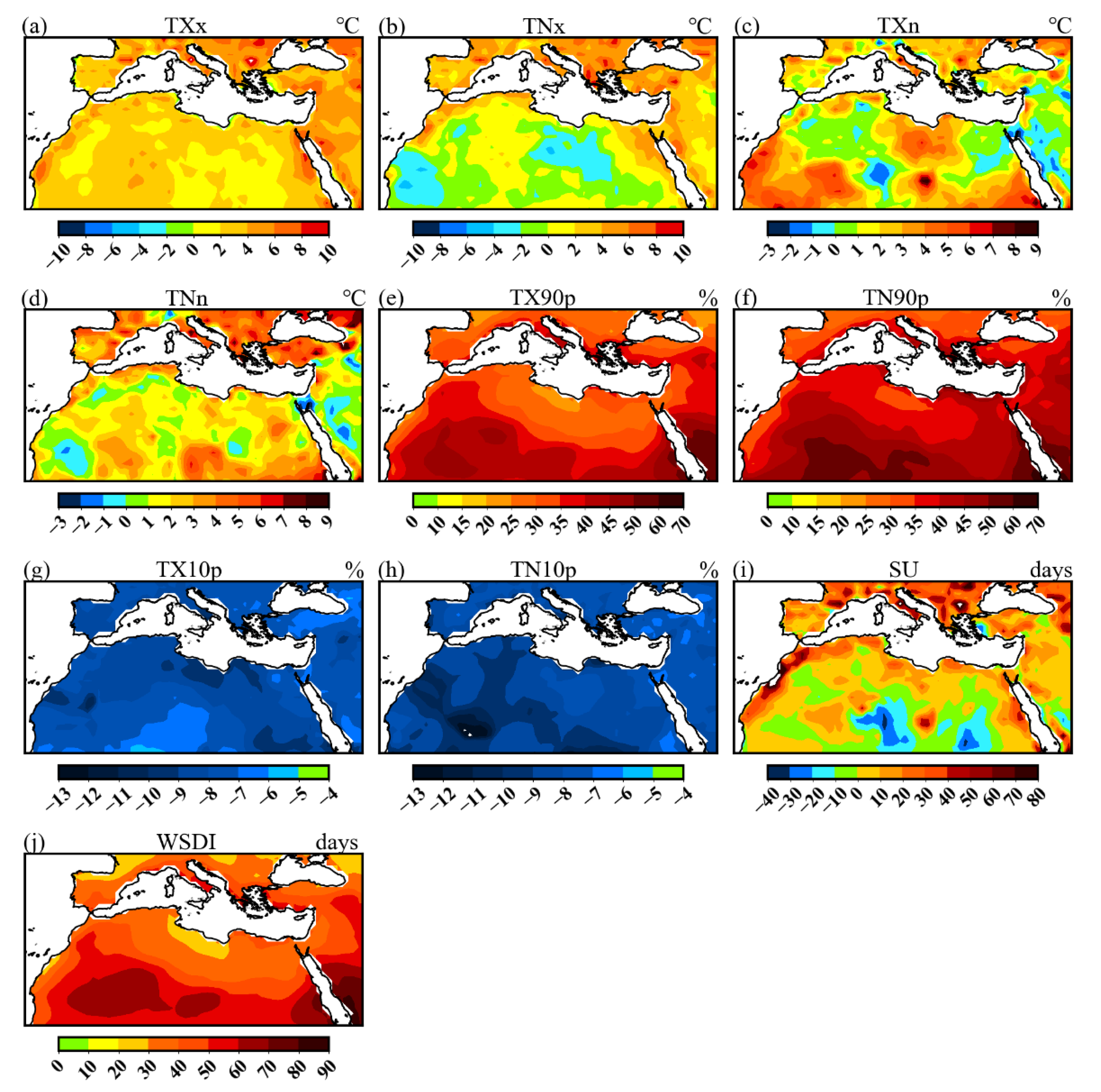
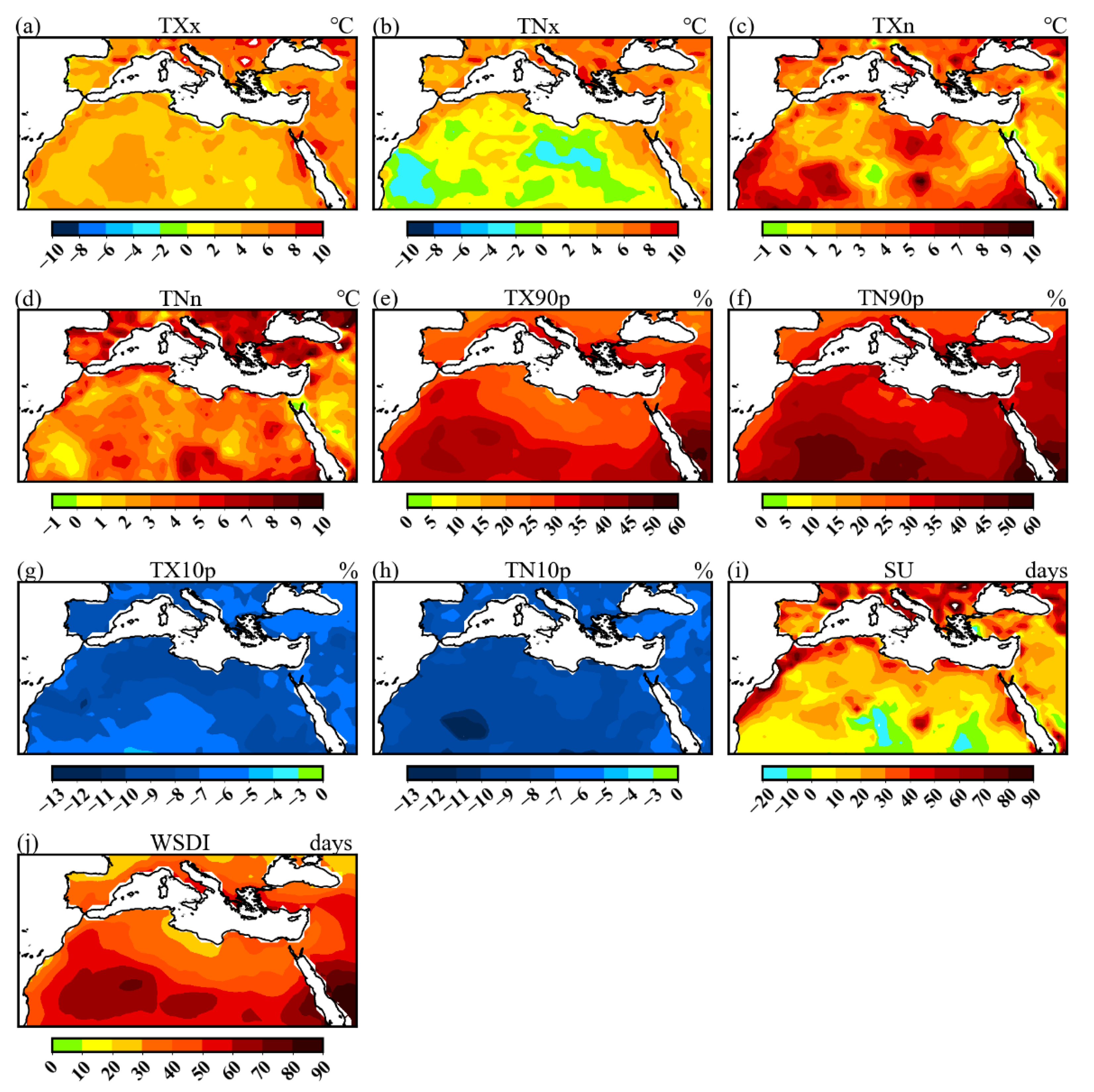
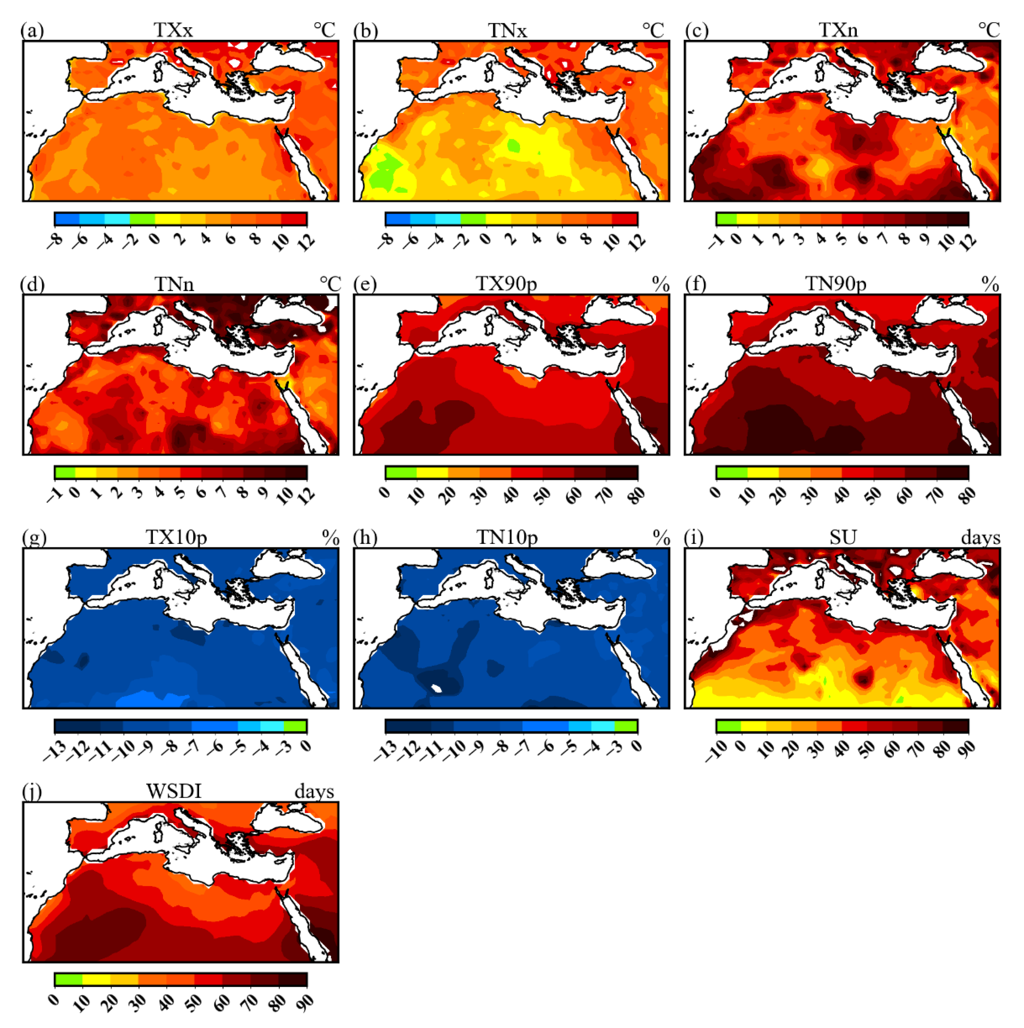
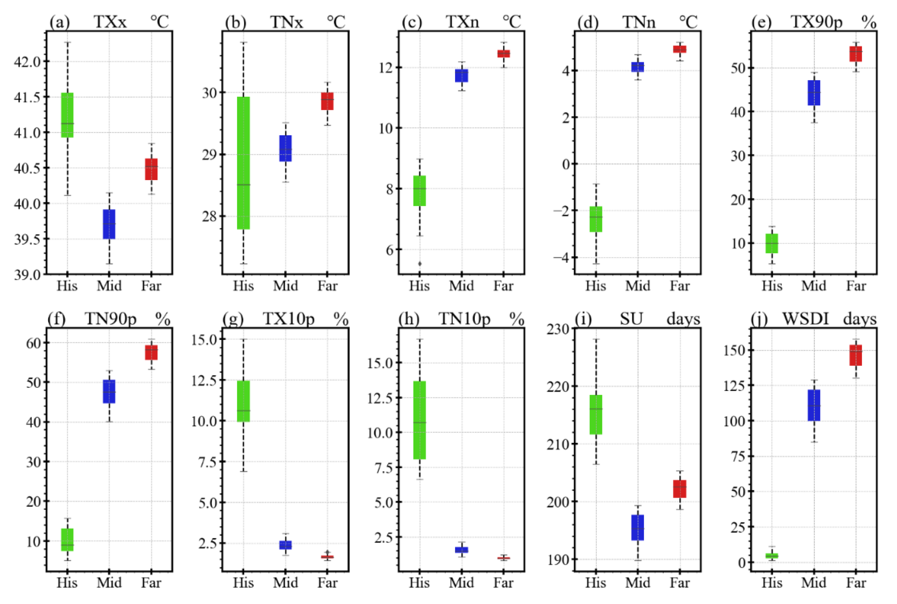
Projected changes in temperature extremes show that the region will experience the highest increase in temperature extremes towards the end of the century under a high emission scenario as compared to mid-century or under a modest mitigation scenario. For instance, TXx, TNx, and TNn depict strong warming over MED compared to SAH during the far-future under the SSP5-8.5 scenario. The projected changes in the warmest nights, TN90p, will be stronger and more impactful as compared to the warmest days, TX90p. Conversely, a sharp decline in cold days (TX10p) and cold nights (TN10p) is projected to occur during mid-century and far-future in both the SSP2-4.5 and SSP5-8.5 scenarios. Simultaneously, the duration indices (SU and WSDI) equally show robust changes over MED as compared to SAH during 2041–2070 and 2071–2100 under the SSP5-8.5 scenario.
(iii)
It is evident that the region will experience statistically significant increasing trends in TXx, TNx, TX90p, TN90p, SU and WSDI during both the mid- and far-future under the SSP2-4.5 and SSP5-8.5 scenarios. Conversely, TX10p and TN10p reveal statistically significant decreasing trends (−0.01 to −0.12/year) over the study region in both timescales and scenarios under consideration. Spatial trends for TXx and TNx depict robust changes over MED under the SSP2-4.5 scenario during the mid-future with a significant positive overall trend and in the far-future with uniform positive trends under the high emission scenario during the two time periods. Overall, these results suggest that the region will experience a high increase in the intensity, duration, and frequency of hot extremes, while the cold extremes will generally decline over the entire study area.

Supplementary Materials

The following supporting information can be downloaded at: https://www.mdpi.com/article/10.3390/atmos13050741/s1.

Author Contributions

The following are individual contributions: B.A., C.O. and H.B.: conceptualization, formal writing, and original draft preparation; H.B. and Z.H.H.: data curation, methodology, visualization; V.O. and R.M.: writing—review and editing, investigation; V.O.: validation; H.B. and A.R.: funding. All authors have read and agreed to the published version of the manuscript.

Funding

This research received no external funding.

Institutional Review Board Statement

Not applicable.

Informed Consent Statement

Not applicable.

Data Availability Statement

All the datasets used in this study are from open-source platforms available via https://esgf-node.llnl.gov/projects/esgf-llnl (accessed on 1 March 2022) for the CMIP6 models.

Acknowledgments

The authors appreciate the data sources for freely providing the data used in this study.

Conflicts of Interest

The authors declare no conflict of interest.

References

  1. Vogel, E.; Donat, M.G.; Alexander, L.V.; Meinshausen, M.; Ray, D.K.; Karoly, D.; Meinshausen, N.; Frieler, K. The effects of climate extremes on global agricultural yields. Environ. Res. Lett. 2019, 14, 054010. [Google Scholar] [CrossRef]
  2. Engelbrecht, F.; Adegoke, J.; Bopape, M.-J.; Naidoo, M.; Garland, R.; Thatcher, M.; McGregor, J.; Katzfey, J.; Werner, M.; Ichoku, C.; et al. Projections of rapidly rising surface temperatures over Africa under low mitigation. Environ. Res. Lett. 2015, 10, 085004. [Google Scholar] [CrossRef]
  3. Ebi, K.L.; Capon, A.; Berry, P.; Broderick, C.; de Dear, R.; Havenith, G.; Honda, Y.; Kovats, R.S.; Ma, W.; Malik, A.; et al. Hot weather and heat extremes: Health risks. Lancet 2021, 398, 698–708. [Google Scholar] [CrossRef]
  4. Niang, I.; Ruppel, O.C.; Abdrabo, M.A.; Essel, A.; Lennard, C.; Padgham, J.; Urquhart, P. Africa. In Climate Change 2014: Impacts, Adaptation and Vulnerability: Part B: Regional Aspects: Working Group II Contribution to the Fifth Assessment Report of the Intergovernmental Panel on Climate Change; Cambridge University Press: Cambridge, UK, 2015; pp. 1199–1266. [Google Scholar]
  5. IPCC. Climate Change 2021: The Physical Science Basis; Contribution of Working Group I to the Sixth Assessment Report of the Intergovernmental Panel on Climate Change; Masson-Delmotte, V., Zhai, P., Pirani, A., Connors, S.L., Péan, C., Berger, S., Caud, N., Chen, Y., Goldfarb, L., Gomis, M.I., et al., Eds.; Cambridge University Press: Cambridge, UK, 2021; in press. [Google Scholar]
  6. Schilling, J.; Hertig, E.; Tramblay, Y.; Scheffran, J. Climate change vulnerability, water resources and social implications in North Africa. Reg. Environ. Chang. 2020, 20, 15. [Google Scholar] [CrossRef] [Green Version]
  7. Nangombe, S.S.; Zhou, T.; Zhang, W.; Zou, L.; Li, D. High-Temperature Extreme Events Over Africa Under 1.5 and 2 °C of Global Warming. J. Geophys. Res. Atmos. 2019, 124, 4413–4428. [Google Scholar] [CrossRef] [Green Version]
  8. Cos, J.; Doblas-Reyes, F.; Jury, M.; Marcos, R.; Bretonnière, P.-A.; Samsó, M. The Mediterranean climate change hotspot in the CMIP5 and CMIP6 projections. Earth Syst. Dyn. Discuss. 2022, 13, 321–340. [Google Scholar] [CrossRef]
  9. Lelieveld, J.; Proestos, Y.; Hadjinicolaou, P.; Tanarhte, M.; Tyrlis, E.; Zittis, G. Strongly increasing heat extremes in the Middle East and North Africa (MENA) in the 21st century. Clim. Chang. 2016, 137, 245–260. [Google Scholar] [CrossRef] [Green Version]
  10. Driouech, F.; Elrhaz, K.; Moufouma-Okia, W.; Arjdal, K.; Balhane, S. Assessing Future Changes of Climate Extreme Events in the CORDEX-MENA Region Using Regional Climate Model ALADIN-Climate. Earth Syst. Environ. 2020, 4, 477–492. [Google Scholar] [CrossRef]
  11. Lange, M.A. Impacts of Climate Change on the Eastern Mediterranean and the Middle East and North Africa Region and the Water–Energy Nexus. Atmosphere 2019, 10, 455. [Google Scholar] [CrossRef] [Green Version]
  12. Linares, C.; Díaz, J.; Negev, M.; Martínez, G.S.; Debono, R.; Paz, S. Impacts of climate change on the public health of the Mediterranean Basin population—Current situation, projections, preparedness and adaptation. Environ. Res. 2020, 182, 109107. [Google Scholar] [CrossRef]
  13. Ozturk, T.; Saygili-Araci, F.; Kurnaz, M. Projected Changes in Extreme Temperature and Precipitation Indices Over CORDEX-MENA Domain. Atmosphere 2021, 12, 622. [Google Scholar] [CrossRef]
  14. Zittis, G.; Hadjinicolaou, P.; Almazroui, M.; Bucchignani, E.; Driouech, F.; El Rhaz, K.; Kurnaz, L.; Nikulin, G.; Ntoumos, A.; Ozturk, T.; et al. Business-as-usual will lead to super and ultra-extreme heatwaves in the Middle East and North Africa. npj Clim. Atmos. Sci. 2021, 4, 20. [Google Scholar] [CrossRef]
  15. Elkouk, A.; Morjani, Z.E.A.E.; Pokhrel, Y.; Chehbouni, A.; Sifeddine, A.; Thober, S.; Bouchaou, L. Multi-model ensemble projections of soil moisture drought over North Africa and the Sahel region under 1.5, 2, and 3 °C global warming. Clim. Chang. 2021, 167, 52. [Google Scholar] [CrossRef]
  16. Bucchignani, E.; Mercogliano, P.; Panitz, H.-J.; Montesarchio, M. Climate change projections for the Middle East–North Africa domain with COSMO-CLM at different spatial resolutions. Adv. Clim. Chang. Res. 2018, 9, 66–80. [Google Scholar] [CrossRef]
  17. Varela, R.; Rodríguez-Díaz, L.; DeCastro, M. Persistent heat waves projected for Middle East and North Africa by the end of the 21st century. PLoS ONE 2020, 15, e0242477. [Google Scholar] [CrossRef] [PubMed]
  18. Bağçaci, S.; Yucel, I.; Duzenli, E.; Yilmaz, M.T. Intercomparison of the expected change in the temperature and the precipitation retrieved from CMIP6 and CMIP5 climate projections: A Mediterranean hot spot case, Turkey. Atmos. Res. 2021, 256, 105576. [Google Scholar] [CrossRef]
  19. Nangombe, S.S.; Zhou, T.; Zhang, W.; Wu, B.; Hu, S.; Zou, L.; Li, D. Record-breaking climate extremes in Africa under stabilized 1.5 °C and 2 °C global warming scenarios. Nat. Clim. Chang. 2018, 8, 375–380. [Google Scholar] [CrossRef]
  20. Seneviratne, S.I.; Hauser, M. Regional Climate Sensitivity of Climate Extremes in CMIP6 Versus CMIP5 Multimodel Ensembles. Earth’s Future 2020, 8, e2019EF001474. [Google Scholar] [CrossRef]
  21. Hawkins, E.; Sutton, R. The Potential to Narrow Uncertainty in Regional Climate Predictions. Bull. Am. Meteorol. Soc. 2009, 90, 1095–1107. [Google Scholar] [CrossRef] [Green Version]
  22. Murphy, J. An Evaluation of Statistical and Dynamical Techniques for Downscaling Local Climate. J. Clim. 1999, 12, 2256–2284. [Google Scholar] [CrossRef]
  23. Wilby, R.L.; Wigley, T.M.L. Precipitation predictors for downscaling: Observed and general circulation model relationships. Int. J. Climatol. 2000, 20, 641–661. [Google Scholar] [CrossRef]
  24. Ahmed, K.F.; Wang, G.; Silander, J.; Wilson, A.; Allen, J.; Horton, R.; Anyah, R. Statistical downscaling and bias correction of climate model outputs for climate change impact assessment in the U.S. northeast. Glob. Planet. Chang. 2013, 100, 320–332. [Google Scholar] [CrossRef] [Green Version]
  25. Moore, K.; Pierson, D.; Pettersson, K.; Schneiderman, E.; Samuelsson, P. Effects of warmer world scenarios on hydrologic inputs to Lake Mälaren, Sweden and implications for nutrient loads. Hydrobiologia 2008, 599, 191–199. [Google Scholar] [CrossRef]
  26. Rasmussen, J.; Sonnenborg, T.O.; Stisen, S.; Seaby, L.P.; Christensen, B.S.B.; Hinsby, K. Climate change effects on irrigation demands and minimum stream discharge: Impact of bias-correction method. Hydrol. Earth Syst. Sci. 2012, 16, 4675–4691. [Google Scholar] [CrossRef] [Green Version]
  27. Lenderink, G.; Buishand, A.; Van Deursen, W. Estimates of future discharges of the river Rhine using two scenario methodologies: Direct versus delta approach. Hydrol. Earth Syst. Sci. 2007, 11, 1145–1159. [Google Scholar] [CrossRef]
  28. Schmidli, J.; Frei, C.; Vidale, P.L. Downscaling from GCM precipitation: A benchmark for dynamical and statistical downscaling methods. Int. J. Clim. 2006, 26, 679–689. [Google Scholar] [CrossRef]
  29. Leander, R.; Buishand, T.A.; van den Hurk, B.J.J.M.; de Wit, M.J.M. Estimated changes in flood quantiles of the river Meuse from resampling of regional climate model output. J. Hydrol. 2008, 351, 331–343. [Google Scholar] [CrossRef]
  30. Block, P.J.; Souza Filho, F.D.A.; Sun, L.; Kwon, H.-H. A Streamflow Forecasting Framework using Multiple Climate and Hydrological Models. JAWRA J. Am. Water Resour. Assoc. 2009, 45, 828–843. [Google Scholar] [CrossRef]
  31. Sun, F.; Roderick, M.L.; Lim, W.H.; Farquhar, G.D. Hydroclimatic projections for the Murray-Darling Basin based on an ensemble derived from Intergovernmental Panel on Climate Change AR4 climate models. Water Resour. Res. 2011, 47, 1–14. [Google Scholar] [CrossRef]
  32. Piani, C.; Weedon, G.; Best, M.; Gomes, S.; Viterbo, P.; Hagemann, S.; Haerter, J.O. Statistical bias correction of global simulated daily precipitation and temperature for the application of hydrological models. J. Hydrol. 2010, 395, 199–215. [Google Scholar] [CrossRef]
  33. Themeßl, M.J.; Gobiet, A.; Heinrich, G. Empirical-statistical downscaling and error correction of regional climate models and its impact on the climate change signal. Clim. Chang. 2012, 112, 449–468. [Google Scholar] [CrossRef]
  34. Gudmundsson, L.; Bremnes, J.B.; Haugen, J.E.; Engen-Skaugen, T. Technical Note: Downscaling RCM precipitation to the station scale using statistical transformations—A comparison of methods. Hydrol. Earth Syst. Sci. 2012, 16, 3383–3390. [Google Scholar] [CrossRef] [Green Version]
  35. Teutschbein, C.; Seibert, J. Bias correction of regional climate model simulations for hydrological climate-change impact studies: Review and evaluation of different methods. J. Hydrol. 2012, 456–457, 12–29. [Google Scholar] [CrossRef]
  36. Chen, J.; Brissette, F.P.; Chaumont, D.; Braun, M. Finding appropriate bias correction methods in downscaling precipitation for hydrologic impact studies over North America. Water Resour. Res. 2013, 49, 4187–4205. [Google Scholar] [CrossRef]
  37. Tabari, H.; Paz, S.M.; Buekenhout, D.; Willems, P. Comparison of statistical downscaling methods for climate change impact analysis on precipitation-driven drought. Hydrol. Earth Syst. Sci. 2021, 25, 3493–3517. [Google Scholar] [CrossRef]
  38. Li, H.; Sheffield, J.; Wood, E. Bias correction of monthly precipitation and temperature fields from Intergovernmental Panel on Climate Change AR4 models using equidistant quantile matching. J. Geophys. Res. Earth Surf. 2010, 115, D10101. [Google Scholar] [CrossRef]
  39. Lionello, P.; Malanotte-Rizzoli, P.; Boscolo, R.; Alpert, P.; Artale, V.; Li, L.; Luterbacher, J.; May, W.; Trigo, R.; Tsimplis, M.; et al. The Mediterranean climate: An overview of the main characteristics and issues. Dev. Earth Environ. Sci. 2006, 4, 1–26. [Google Scholar] [CrossRef]
  40. Nouaceur, Z.; Murarescu, O. Rainfall Variability and Trend Analysis of Annual Rainfall in North Africa. Int. J. Atmos. Sci. 2016, 2016, 7230450. [Google Scholar] [CrossRef]
  41. Babaousmail, H.; Hou, R.; Gnitou, G.T.; Ayugi, B. Novel statistical downscaling emulator for precipitation projections using deep Convolutional Autoencoder over Northern Africa. J. Atmos. Sol.-Terr. Phys. 2021, 218, 105614. [Google Scholar] [CrossRef]
  42. Iturbide, M.; Gutiérrez, J.M.; Alves, L.M.; Bedia, J.; Cerezo-Mota, R.; Cimadevilla, E.; Cofiño, A.S.; Di Luca, A.; Faria, S.H.; Gorodetskaya, I.V.; et al. An update of IPCC climate reference regions for subcontinental analysis of climate model data: Definition and aggregated datasets. Earth Syst. Sci. Data Discuss. 2020, 12, 2959–2970. [Google Scholar] [CrossRef]
  43. Fan, Y.; van den Dool, H. A global monthly land surface air temperature analysis for 1948–present. J. Geophys. Res. Atmos. 2008, 113, D01103. [Google Scholar] [CrossRef]
  44. Coppola, E.; Raffaele, F.; Giorgi, F.; Giuliani, G.; Xuejie, G.; Ciarlo, J.M.; Sines, T.R.; Torres-Alavez, J.A.; Das, S.; di Sante, F.; et al. Climate hazard indices projections based on CORDEX-CORE, CMIP5 and CMIP6 ensemble. Clim. Dyn. 2021, 57, 1293–1383. [Google Scholar] [CrossRef]
  45. Eyring, V.; Bony, S.; Meehl, G.A.; Senior, C.A.; Stevens, B.; Stouffer, R.J.; Taylor, K.E. Overview of the Coupled Model Intercomparison Project Phase 6 (CMIP6) experimental design and organization. Geosci. Model Dev. 2016, 9, 1937–1958. [Google Scholar] [CrossRef] [Green Version]
  46. O’Neill, B.C.; Tebaldi, C.; van Vuuren, D.P.; Eyring, V.; Friedlingstein, P.; Hurtt, G.; Knutti, R.; Kriegler, E.; Lamarque, J.-F.; Lowe, J.; et al. The Scenario Model Intercomparison Project (ScenarioMIP) for CMIP6. Geosci. Model Dev. 2016, 9, 3461–3482. [Google Scholar] [CrossRef] [Green Version]
  47. Zhang, X.; Alexander, L.; Hegerl, G.C.; Jones, P.; Tank, A.K.; Peterson, T.C.; Trewin, B.; Zwiers, F.W. Indices for monitoring changes in extremes based on daily temperature and precipitation data. Wires Clim. Chang. 2011, 2, 851–870. [Google Scholar] [CrossRef]
  48. Ongoma, V.; Chen, H.; Gao, C.; Nyongesa, A.M.; Polong, F. Future changes in climate extremes over Equatorial East Africa based on CMIP5 multimodel ensemble. Nat. Hazards 2018, 90, 901–920. [Google Scholar] [CrossRef]
  49. Iyakaremye, V.; Zeng, G.; Zhang, G. Changes in extreme temperature events over Africa under 1.5 and 2.0 °C global warming scenarios. Int. J. Climatol. 2021, 41, 1506–1524. [Google Scholar] [CrossRef]
  50. Iyakaremye, V.; Zeng, G.; Yang, X.; Zhang, G.; Ullah, I.; Gahigi, A.; Vuguziga, F.; Asfaw, T.G.; Ayugi, B. Increased high-temperature extremes and associated population exposure in Africa by the mid-21st century. Sci. Total Environ. 2021, 790, 148162. [Google Scholar] [CrossRef]
  51. Zhao, Y.; Qian, C.; Zhang, W.; He, D.; Qi, Y. Extreme temperature indices in Eurasia in a CMIP6 multi-model ensemble: Evaluation and projection. Int. J. Clim. 2021, 41, 5368–5385. [Google Scholar] [CrossRef]
  52. Gupta, R.; Bhattarai, R.; Mishra, A. Development of Climate Data Bias Corrector (CDBC) Tool and Its Application over the Agro-Ecological Zones of India. Water 2019, 11, 1102. [Google Scholar] [CrossRef] [Green Version]
  53. Klemeš, V. Operational testing of hydrological simulation models. Hydrol. Sci. J. 1986, 31, 13–24. [Google Scholar] [CrossRef]
  54. Knutti, R.; Furrer, R.; Tebaldi, C.; Cermak, J.; Meehl, G.A. Challenges in Combining Projections from Multiple Climate Models. J. Clim. 2010, 23, 2739–2758. [Google Scholar] [CrossRef] [Green Version]
  55. Sanderson, B.; Knutti, R.; Caldwell, P. Addressing Interdependency in a Multimodel Ensemble by Interpolation of Model Properties. J. Clim. 2015, 28, 5150–5170. [Google Scholar] [CrossRef]
  56. Hamed, K.H.; Rao, A.R. A modified Mann-Kendall trend test for autocorrelated data. J. Hydrol. 1998, 204, 182–196. [Google Scholar] [CrossRef]
  57. Sheffield, J.; Wood, E.F.; Roderick, M.L. Little change in global drought over the past 60 years. Nature 2012, 491, 435–438. [Google Scholar] [CrossRef]
  58. IPCC. Climate Change 2013—The Physical Science Basis; Contribution of Working Group I to the Fifth Assessment Report of the Intergovernmental Panel on Climate Change; Stocker, T.F., Qin, D., Plattner, G.-K., Tignor, M., Allen, S.K., Boschung, J., Nauels, A., Xia, Y., Bex, V., Midgley, P.M., Eds.; Cambridge University Press: Cambridge, UK; New York, NY, USA, 2013; 1535p. [Google Scholar] [CrossRef] [Green Version]
  59. Haile, G.G.; Tang, Q.; Hosseini-Moghari, S.; Liu, X.; Gebremicael, T.G.; Leng, G.; Kebede, A.; Xu, X.; Yun, X. Projected Impacts of Climate Change on Drought Patterns Over East Africa. Earth’s Future 2020, 8, e2020EF001502. [Google Scholar] [CrossRef]
  60. Maraun, D. When will trends in European mean and heavy daily precipitation emerge? Environ. Res. Lett. 2013, 8, 014004. [Google Scholar] [CrossRef]
  61. Miao, C.; Su, L.; Sun, Q.; Duan, Q. A nonstationary bias-correction technique to remove bias in GCM simulations. J. Geophys. Res. Atmos. 2016, 121, 5718–5735. [Google Scholar] [CrossRef]
  62. Ayugi, B.; Tan, G.; Ruoyun, N.; Babaousmail, H.; Ojara, M.; Wido, H.; Mumo, L.; Ngoma, N.H.; Nooni, I.K.; Ongoma, V. Quantile Mapping Bias Correction on Rossby Centre Regional Climate Models for Precipitation Analysis over Kenya, East Africa. Water 2020, 12, 801. [Google Scholar] [CrossRef] [Green Version]
  63. Dosio, A.; Lennard, C.; Spinoni, J. Projections of indices of daily temperature and precipitation based on bias-adjusted CORDEX-Africa regional climate model simulations. Clim. Chang. 2022, 170, 13. [Google Scholar] [CrossRef]
  64. Mondal, S.K.; Huang, J.; Wang, Y.; Su, B.; Kundzewicz, Z.W.; Jiang, S.; Zhai, J.; Chen, Z.; Jing, C.; Jiang, T. Changes in extreme precipitation across South Asia for each 0.5 °C of warming from 1.5 °C to 3.0°C above pre-industrial levels. Atmos. Res. 2021, 266, 105961. [Google Scholar] [CrossRef]
  65. Kharin, V.V.; Zwiers, F.W.; Zhang, X.; Wehner, M. Changes in temperature and precipitation extremes in the CMIP5 ensemble. Clim. Chang. 2013, 119, 345–357. [Google Scholar] [CrossRef]
  66. Li, C.; Zwiers, F.; Zhang, X.; Li, G.; Sun, Y.; Wehner, M. Changes in Annual Extremes of Daily Temperature and Precipitation in CMIP6 Models. J. Clim. 2021, 34, 3441–3460. [Google Scholar] [CrossRef]
  67. Zollo, A.L.; Rillo, V.; Bucchignani, E.; Montesarchio, M.; Mercogliano, P. Extreme temperature and precipitation events over Italy: Assessment of high-resolution simulations with COSMO-CLM and future scenarios. Int. J. Clim. 2016, 36, 987–1004. [Google Scholar] [CrossRef] [Green Version]
  68. Tomozeiu, R.; Agrillo, G.; Cacciamani, C.; Pavan, V. Statistically downscaled climate change projections of surface temperature over Northern Italy for the periods 2021–2050 and 2070–2099. Nat. Hazards 2014, 72, 143–168. [Google Scholar] [CrossRef]
  69. Abaurrea, J.; Asín, J.; Cebrián, A. Modelling the occurrence of heat waves in maximum and minimum temperatures over Spain and projections for the period 2031-60. Glob. Planet. Chang. 2018, 161, 244–260. [Google Scholar] [CrossRef] [Green Version]
  70. Cardoso, R.M.; Soares, P.M.M.; Lima, D.C.A.; Miranda, P.M.A. Mean and extreme temperatures in a warming climate: EURO CORDEX and WRF regional climate high-resolution projections for Portugal. Clim. Dyn. 2018, 52, 129–157. [Google Scholar] [CrossRef]
  71. Cardell, M.F.; Amengual, A.; Romero, R.; Ramis, C. Future extremes of temperature and precipitation in Europe derived from a combination of dynamical and statistical approaches. Int. J. Clim. 2020, 40, 4800–4827. [Google Scholar] [CrossRef]
  72. Claussen, M.; Mysak, L.; Weaver, A.; Crucifix, M.; Fichefet, T.; Loutre, M.F.; Weber, S.; Alcamo, J.; Alexeev, V.; Berger, A.; et al. Earth system models of intermediate complexity: Closing the gap in the spectrum of climate system models. Clim. Dyn. 2002, 18, 579–586. [Google Scholar] [CrossRef] [Green Version]
  73. Wang, L.; Hardiman, S.C.; Bett, P.E.; Comer, R.E.; Kent, C.; Scaife, A.A. What chance of a sudden stratospheric warming in the southern hemisphere? Environ. Res. Lett. 2020, 15, 104038. [Google Scholar] [CrossRef]
  74. Taylor, K.E.; Stouffer, R.J.; Meehl, G.A. An Overview of CMIP5 and the Experiment Design. Bull. Am. Meteorol. Soc. 2012, 93, 485–498. [Google Scholar] [CrossRef] [Green Version]
  75. Zhu, H.; Jiang, Z.; Li, J.; Li, W.; Sun, C.; Li, L. Does CMIP6 Inspire More Confidence in Simulating Climate Extremes over China? Adv. Atmos. Sci. 2020, 37, 1119–1132. [Google Scholar] [CrossRef]
  76. Xin, X.; Wu, T.; Zhang, J.; Yao, J.; Fang, Y. Comparison of CMIP6 and CMIP5 simulations of precipitation in China and the East Asian summer monsoon. Int. J. Clim. 2020, 40, 6423–6440. [Google Scholar] [CrossRef] [Green Version]
  77. Lun, Y.; Liu, L.; Cheng, L.; Li, X.; Li, H.; Xu, Z. Assessment of GCMs simulation performance for precipitation and temperature from CMIP5 to CMIP6 over the Tibetan Plateau. Int. J. Clim. 2021, 41, 3994–4018. [Google Scholar] [CrossRef]
  78. Luo, N.; Guo, Y.; Chou, J.; Gao, Z. Added value of CMIP6 models over CMIP5 models in simulating the climatological precipitation extremes in China. Int. J. Clim. 2021, 42, 1148–1164. [Google Scholar] [CrossRef]
  79. Ayugi, B.; Zhihong, J.; Zhu, H.; Ngoma, H.; Babaousmail, H.; Rizwan, K.; Dike, V. Comparison of CMIP6 and CMIP5 models in simulating mean and extreme precipitation over East Africa. Int. J. Clim. 2021, 41, 6474–6496. [Google Scholar] [CrossRef]
  80. Nastos, P.T.; Kapsomenakis, J. Regional climate model simulations of extreme air temperature in Greece. Abnormal or common records in the future climate? Atmos. Res. 2015, 152, 43–60. [Google Scholar] [CrossRef]
  81. Weber, T.; Haensler, A.; Rechid, D.; Pfeifer, S.; Eggert, B.; Jacob, D. Analyzing Regional Climate Change in Africa in a 1.5, 2, and 3°C Global Warming World. Earth’s Future 2018, 6, 643–655. [Google Scholar] [CrossRef]
  82. Giorgi, F.; Coppola, E.; Raffaele, F.; Diro, G.T.; Fuentes-Franco, R.; Giuliani, G.; Mamgain, A.; Llopart, M.; Mariotti, L.; Torma, C. Changes in extremes and hydroclimatic regimes in the CREMA ensemble projections. Clim. Chang. 2014, 125, 39–51. [Google Scholar] [CrossRef]
  83. Majdi, F.; Hosseini, S.A.; Karbalaee, A.; Kaseri, M.; Marjanian, S. Future projection of precipitation and temperature changes in the Middle East and North Africa (MENA) region based on CMIP6. Arch. Meteorol. Geophys. Bioclimatol. Ser. B 2022, 147, 1249–1262. [Google Scholar] [CrossRef]
  84. Tebaldi, C.; Knutti, R. The use of the multi-model ensemble in probabilistic climate projections. Philos. Trans. R. Soc. A Math. Phys. Eng. Sci. 2007, 365, 2053–2075. [Google Scholar] [CrossRef] [PubMed]
  85. Knutti, R.; Rugenstein, M.A.A.; Hegerl, G. Beyond equilibrium climate sensitivity. Nat. Geosci. 2017, 10, 727–736. [Google Scholar] [CrossRef]
  86. Dunn, R.J.H.; Alexander, L.V.; Donat, M.G.; Zhang, X.; Bador, M.; Herold, N.; Lippmann, T.; Allan, R.; Aguilar, E.; Barry, A.A.; et al. Development of an Updated Global Land In Situ-Based Data Set of Temperature and Precipitation Extremes: HadEX3. J. Geophys. Res. Atmos. 2020, 125, e2019JD032263. [Google Scholar] [CrossRef]
  87. Almazroui, M.; Saeed, F.; Saeed, S.; Ismail, M.; Ehsan, M.A.; Islam, M.N.; Abid, M.A.; O’Brien, E.; Kamil, S.; Rashid, I.U.; et al. Projected Changes in Climate Extremes Using CMIP6 Simulations Over SREX Regions. Earth Syst. Environ. 2021, 5, 481–497. [Google Scholar] [CrossRef]
Figure 1. Spatial plot of mean temperature during 1979 to 2014 over the study domain: Mediterranean (MED) and Sahara (SAH), based on the Climate Prediction Centre (CPC). The study region is demarcated (dashed black line) following Iturbide et al. [42].
Atmosphere 13 00741 g001
Figure 2. Flowchart of model bias correction procedure based on sample split testing technique.
Atmosphere 13 00741 g002
Figure 3. Empirical cumulative distribution function (ECDF) of GCMs and their multi-model mean ensemble (MME) (black dotted line) before (a) and after (b) bias correction, relative to the CPC data (red dotted line).
Atmosphere 13 00741 g003
Figure 4. Spatial distribution of warm spell duration index (WSDI) difference from the CMIP6 GCMs (Table 1) and their MME during 1979–2014. The first plot shows the climatology of (WSDI) from CPC. The model difference is calculated as model (before correction) minus CPC.
Atmosphere 13 00741 g004
Figure 5. Spatial distribution of warm spell duration index (WSDI) difference from the CMIP6 GCMs and their MME during 1979–2014. The first plot shows the climatology of WSDI from CPC. The model difference is calculated as model (after correction) minus CPC.
Atmosphere 13 00741 g005
Figure 6. Projected changes in extreme temperature from multi-model ensemble mean CMIP6 GCMs bias-adjusted data during the mid-future (2041–2070) relative to the baseline period (1995–2014) for the SSP2-4.5 scenario. The indices reflect the intensity (TXx, TNx, TXn and TNn) (ad), frequency (TX90p, TN90p, TX10p, and TN10p) (eh) and duration (SU and WSDI) (i,j) of the extreme events.
Atmosphere 13 00741 g006
Figure 7. Same as Figure 6, but for the period 2071–2100.
Atmosphere 13 00741 g007
Figure 8. Projected changes in extreme temperature from multi-model ensemble mean CMIP6 GCMs bias-adjusted data during the mid-future (2041–2070) relative to the baseline period (1995–2014) for the SSP5-8.5 scenario. The indices reflect the intensity (TXx, TNx, TXn and TNn) (ad), frequency (TX90p, TN90p, TX10p, and TN10p) (eh) and duration (SU and WSDI) (i,j) of the extreme events.
Atmosphere 13 00741 g008
Figure 9. Same as Figure 8, but for the period 2071–2100.
Atmosphere 13 00741 g009
Figure 10. Time series of projected extreme temperature anomalies spatially averaged over the study domain for SSP2-4.5 (blue) and SSP5-8.5 scenario (red). The anomaly is calculated relative to the mean of baseline period. The green and purple dotted lines indicate the mid- (2041–2070) and far-future period (2071–2100), respectively. The blue and red shadings are the corresponding model spread about the MME.
Atmosphere 13 00741 g010
Figure 11. Spatial trends of extreme temperature from the multi-model ensemble mean of CMIP6 GCMs bias-adjusted data for the mid-future (2041–2070) relative to the baseline period (1995–2014) for the SSP2-4.5 scenario. The indices reflect the intensity (TXx, TNx, TXn and TNn) (ad), frequency (TX90p, TN90p, TX10p, and TN10p) (eh) and duration (SU and WSDI) (i,j) of the extreme events.
Atmosphere 13 00741 g011
Figure 12. Same as Figure 11, but for the far-future (2071–2100).
Atmosphere 13 00741 g012
Figure 13. Spatial trends of extreme temperature from the multi-model ensemble mean of CMIP6 GCMs bias-adjusted data for the mid-future (2041–2070) relative to the baseline period (1995–2014) for the SSP5-8.5 scenario. The indices reflect the intensity (TXx, TNx, TXn and TNn) (ad), frequency (TX90p, TN90p, TX10p, and TN10p) (eh) and duration (SU and WSDI) (i,j) of the extreme events.
Atmosphere 13 00741 g013
Figure 14. Same as Figure 13, but for the far-future (2071–2100).
Atmosphere 13 00741 g014
Figure 15. Projected changes in extreme temperature spatially averaged over the study domain during the mid- (2041–2070) and far-future (2071–2100) relative to the baseline period (1995–2014) for the SSP2-4.5 scenario. The indices reflect the intensity (TXx, TNx, TXn and TNn) (ad), frequency (TX90p, TN90p, TX10p, and TN10p) (eh) and duration (SU and WSDI) (i,j) of the extreme events. For each box plot, the horizontal line represents the median and central uncertainty range of the temperature index across the CMIP6 MME. The whiskers extend to the 10 and 90% uncertainty range.
Atmosphere 13 00741 g015
Figure 16. Same as Figure 15, but for the SSP5-8.5 scenario.
Atmosphere 13 00741 g016
Table 1. List of the CMIP6 General circulation models (GCMs) models used in this study.
No. Model NameModelling GroupAtmosphericResolution (lon × lat)
1ACCESS-CM2Commonwealth Scientific and Industrial Research Organisation/Australia1.25° × 1.875°
2ACCESS-ESM1-5Commonwealth Scientific and Industrial Research Organization and Bureau of Meteorology/Australia1.25° × 1.875°
3BCC-CSM2-MRBeijing Climate Center/China1.125° × 1.125°
4CanESM5Canadian Centre for Climate Modelling and Analysis/Canada2.8° × 2.8°
5CNRM-CM6-1Centre National de Recherches Météorologiques–Centre Européen de Recherche et de Formation Avancée en Calcul Scientifique/France1.4° × 1.4°
6CNRM-ESM2-1Centre National de Recherches Météorologiques–Centre Européen de Recherche et de Formation Avancée en Calcul Scientifique/France1.4° × 1.4°
7EC-Earth3EC-EARTH consortium/Europe0.7° × 0.7°
8EC-Earth3-vegEC-EARTH consortium/Europe0.7° × 0.7°
9FGOALS-g3Chinese Academy of Sciences/China2.25° × 2°
10GFDL-CM4NOAA Geophysical Fluid Dynamics Laboratory/USA1° × 1.25°
11GFDL-ESM4NOAA Geophysical Fluid Dynamics Laboratory/USA1° × 1.25°
12HadGEM3-GC31-LLMet Office Hadley Centre/UK1.25° × 1.875°
13INM-CM4-8Institute for Numerical Mathematics/Russian Academy of Science/Russia1.5° × 2°
14INM-CM5-0Institute for Numerical Mathematics/Russian Academy of Science/Russia1.5° × 2°
15MIROC6Japan Agency for Marine-Earth Science and Technology, Atmosphere and Ocean Research Institute, The University of Tokyo, National Institute for Environmental Studies, and RIKEN Center for computational Science/Japan1.4° × 1.4°
16MIROC-ES2LJapan Agency for Marine-Earth Science and Technology, Atmosphere and Ocean Research Institute, The University of Tokyo, National Institute for Environmental Studies, and RIKEN Center for Computational Science/Japan1.4° × 1.4°
17MPI-ESM1-2-HRMax Planck Institute for Meteorology/Germany0.9375° × 0.9375°
18MPI-ESM1-2-LRMax Planck Institute for Meteorology/Germany1.875° × 1.875°
19MRI-ESM2-0Meteorological Research Institute/Japan1.125° × 1.125°
20NESM3Nanjing University of Information Science and Technology/China1.875° × 1.875°
21NorESM2-LMNorwegian Climate Centre/Norway1.875° × 2.5°
22NorESM2-MMNorwegian Climate Centre/Norway0.9375° × 1.25°
23UKESM1-0-LLMet Office Hadley Centre/UK1.25° × 1.875°
Table 2. Names, abbreviations, definitions, and units of climate indices used in the study.
IDAbbreviationDefinitionUnits
TXxMax TmaxAnnual maximum value of daily maximum temperature °C
TNxMax TminAnnual maximum value of daily minimum temperature°C
TXnMin TmaxAnnual minimum value of daily maximum temperature°C
TNnMin TminAnnual minimum value of daily minimum temperature °C
TX90pWarm daysPercentage of days where daily max temp > 90th percentile%
TN90pWarm nightsPercentage of days where daily min temp > 90th percentile%
TX10pCold daysPercentage of days where daily max temp < 10th percentile%
TN10pCold nightsPercentage of days where daily min temp < 10th percentile%
SUSummer daysAnnual number of days where daily max temp > 25℃ days
WSDIWarm spell Annual number of days, in interval of six consecutive days, where daily max temp > 90th percentile of base perioddays
Table 3. Modified Mann–Kendall Z values for significance test of various temperature indices during mid-future (2041–2070) and far-future (2071–2100) under SSP2-4.5 and SSP5-8.5 over SAH and MED region. The bold denotes significant trends at a 95% confidence level. The asterisk (*) denotes significant at a 99% confidence level.
MMETXxTNxTXnTNnTX90pTN90pTX10pTN10pSUWSDI
SAHSSP2-4.5 Mid3.393.250.891.254.173.96−2.75−2.283.784
SSP2-4.5 Far3.183.281.681.962.823.39−2.43−1.572.533.1
MEDSSP5-8.5 Mid5.17 *5.28 *2.782.855.85 *5.57 *−4.25−4.15.03 *5.99 *
SSP5-8.5 Far5.6 *5.53 *3.714.176.176.1−4.67−4.145.85 *6.07 *
Publisher’s Note: MDPI stays neutral with regard to jurisdictional claims in published maps and institutional affiliations.

