Aerosol Optical Thickness Retrieval in Presence of Cloud: Application to S3A/SLSTR Observations

Abstract

The Combined Inversion of Surface and AeRosols (CISAR) algorithm for the joint retrieval of surface and aerosol single scattering properties has been further developed in order to extend the retrieval to clouds and overcome the need for an external cloud mask. Pixels located in the transition zone between pure cloud and pure aerosol are often discarded by both aerosol and cloud algorithms, despite being essential for studying aerosol–cloud interactions, which still represent the largest source of uncertainty in climate predictions. The proposed approach aims at filling this gap and deepening the understanding of aerosol properties in cloudy environments. The new CISAR version is applied to Sentinel-3A/SLSTR observations and evaluated against different satellite products and ground measurements. The spatial coverage is greatly improved with respect to algorithms processing only pixels flagged as clear sky by the SLSTR cloud mask. The continuous retrieval of aerosol properties without any safety zone around clouds opens new possibilities for studying aerosol properties in cloudy environments.

1. Introduction

Aerosol particles play a fundamental role in the Earth’s climate by reflecting and absorbing the incoming solar radiation. Anthropogenic aerosols have been identified as one of the main contributors to climate forcing, and their interactions with clouds continue to contribute the largest uncertainty to the total radiative forcing (RF) estimate [1]. Aerosols, or, more precisely, fine mode (FM) aerosol particles, can act as cloud condensation nuclei (CCN), altering cloud properties and their radiative effects. Moreover, aerosols have an impact on human health, with ambient air pollution causing over 4 million premature deaths yearly [2]. Dust events such as, for instance, sand storms coming from the Sahara region, affect not only the climate and human health, but also affect the correct functioning of solar panels installation. Given the above considerations, it is clear that observing and understanding aerosol properties is a crucial point for the remote sensing community.

Normally, aerosol retrieval from satellite remote sensing relies on a preliminary cloud masking algorithm to separate cloudy and clear sky observations; the retrieval is thus performed only on clear-sky pixels. An experiment performed in the framework of the European Space Agency (ESA) aerosol climate change initiative (CCI) project showed how applying different cloud masks to the same aerosol retrieval algorithm can strongly impact the algorithm performances [3]. Cloud detection algorithms are usually based on physical principles, but threshold values used to identify cloudy and cloud-free pixels can vary according to the application. An accurate cloud masking can strongly improve the aerosol retrieval as it reduces the possibility of cloud contamination, which probability increases at coarser resolutions [4], and the adjacency effect, which could lead to an enhancement of the measured top-of-atmosphere (TOA) bidirectional reflectance factor (BRF) and in turn to an overestimated aerosol optical thickness (AOT). Because of the TOA BRF enhancement due to adjacent clouds, the aerosol retrieval is strongly dependent on the quality of the cloud mask used to classify cloud-free pixels [3].

To minimize the effect of the TOA BRF enhancement and thus the overestimation of low AOT, the cloud mask in aerosol retrieval applications normally takes into account a safety zone around cloud particles [5]. For instance, in the above-mentioned aerosol-CCI experiment, this safety zone had an extent of 10 km. However, even after such a conservative cloud masking, it is shown that the retrieved AOT tends to be higher in the vicinity of clouds [6,7]. Analysing MODIS data, [8] found that the retrieved AOT was 25% larger, with cloud fraction (CF) of 0.8–0.9, than in relatively cloud-free conditions (CF = 0.1–0.2). Moreover, due to such a conservative cloud mask, a large amount of pixels are “lost”, discarded by both aerosol and cloud algorithms. Ref. [9] calculated that in the case of MODIS, 20% of all pixels are discarded by both aerosol and cloud algorithms. Given the primary role of aerosol–cloud interactions (ACI) in the uncertainty estimation of radiative forcing by climate change models, the transition zone between clear and cloudy sky is currently receiving increasing attention [6,10,11]. Aerosol particles near clouds become more hydrating and swell in size, resulting in increased AOT [12]. Clouds are also sources of aerosols, generating new particles through aqueous chemistry and subsequent evaporation; these particles may have very different optical properties than those particles initially available [13]. Given the above considerations, this transition zone and the changes in aerosol properties in the vicinity of clouds is not necessarily an artefact and should be studied extensively [14,15]. Since AOT is normally retrieved only in cloud-free conditions, the total AOT measured from satellites is most likely underestimated, with a subsequent underestimation of the aerosol direct radiative effect [16]. On the other hand, processing pixels in the vicinity of clouds could lead to a significant overestimation of the AOT, as any enhancement of the TOA BRF in these pixels would be attributed to aerosols. It should be noted here, however, that in inversion algorithms based on 1D radiative transfer models (RTMs), any 3D effects between clouds and clear-sky pixels cannot be correctly characterized.

The new version of the Combined Inversion of Surface and AeRosols (CISAR) algorithm [17,18] presented in this paper addresses some of the issues related to clouds in the aerosols retrieval. After a short training period, the new algorithm no longer relies on an external cloud mask, meaning that cloudy observations and pixels located in the safety zone between clear and cloudy sky will be processed with the same radiative assumptions as cloud-free pixels. Such a product could improve our understanding of aerosol properties in the vicinity of clouds. In addition, high aerosol events are often misclassified as clouds from several cloud masking algorithms; without relying on an external cloud mask, CISAR is capable of retrieving such events. Section 2 describes the data used for this study and the new features of the CISAR algorithm with respect to [17], which allows CISAR to address the new challenges introduced by the processing of cloudy pixels. A case study over a dust storm originating from Sahara and moving towards the Caribbean islands will be presented in Section 3, where CISAR retrieval will be evaluated against cross-satellite products and ground observations.

2. Data and Method

2.1. The SLSTR Instrument

The Sea and Land Surface Temperature Radiometer (SLSTR) instrument, designed to maintain continuity with the (A)ATSR series of instruments, is one of the instruments onboard Sentinel-3, an Earth constellation developed by ESA in the framework of the Copernicus program. Despite being primarily an ocean mission, Sentinel-3 is proven suitable for atmospheric and land applications. The constellation consists of two satellites: Sentinel-3A, launched on 16 February 2016, and Sentinel-3B, launched on 25 April 2018. The Sentinel-3 satellites are polar-orbiting, flying at an altitude of 815 km with a local equatorial crossing time of 10:00 a.m. SLSTR covers nine spectral bands located between 0.55 $\mathsf{\mu }$m and 12 $\mathsf{\mu }$m, of which only the six reflective bands (S1 to S6) are considered in this study. The central wavelengths of bans S1 to S6 are reported in

Table 1. Central wavelength of SLSTR bands S1 to S6.

Band	Central Wavelength ($\mathsf{\mu }$m)
S1	0.554
S2	0.659
S3	0.868
S4	1.374
S5	1.613
S6	2.225

. Of particular interest is the band S4, centered at 1.37 $\mathsf{\mu }$m on a pick of water vapor absorption. This band is used for cirrus detection over land. One of the interesting features of the instrument in the framework of atmospheric application is the dual view. Images are acquired at nadir and at an angle of 55${}^{°}$, with swath widths equal to 1420 km and 750 km, respectively. The dual view of the SLSTR instrument allows a revisit time of 1.9 days at the equator and 1.5 days at latitudes higher than 30${}^{°}$. However, the oblique view is in the opposite direction compared to (A)ATSR, hence in the backscattering direction in the Northern Hemisphere [19]. The impact of this geometric configuration on the information content associated with the satellite observation is analyzed in Section 2.3.1.

This study is based on SLSTR onboard Sentinel-3A acquisitions, aggregated at 10 km super-pixels. The aggregation still exploits the summary cloud mask in the SLSTR Level-1 product as follows:

• If the 80% of sub-pixels are cloud-free, only cloud-free observations are aggregated and the cloud mask is set to 0.
• If the 80% of sub-pixels are cloudy, only cloudy observations are aggregated and the cloud mask is set to 1.
• Otherwise, all pixels are aggregated and the cloud mask is a number between 0 and 1, indicating the percentage of cloudy pixels.

2.2. The CISAR Algorithm

The CISAR algorithm has been developed to address the limitations of a look-up-table (LUT)-based approach and the consistency issues that arise from retrieving different Earth system components with dedicated algorithms. CISAR is based on the online inversion of a fast RTM, which allows the retrieval of surface reflectance and aerosol single scattering properties (optical thickness, single scattering albedo, and asymmetry factor), with continuous variation of the state variable in the solution space [17]. The inversion is performed with an optimal estimation (OE) approach, a strict mathematical framework that seeks the best balance between the information coming from the observation and any prior information on the observed system. Satellite observations are accumulated during the so-called accumulation period, the length of which varies according to the satellite characteristics. During the accumulation period, the surface reflectance properties are considered constant, while the aerosol and cloud single scattering properties are retrieved at each satellite acquisition.

The algorithm is applicable to any sensor acquiring observations in the visible spectral region, and its performances, when applied to radiometers flying at different orbits (polar-orbiting and geostationary), have been analyzed in [18]. Similar to other aerosol retrieval algorithms [20,21], CISAR tends to overestimate low AOTs. Identifying the cloud effects as one of the causes of this overestimation, and given the strong dependency of aerosol retrieval on the cloud masking [3], CISAR has been extended to the retrieval of cloud single scattering properties, overcoming the need for an external cloud mask. This innovative approach aims at improving the spatial coverage of aerosol products, reducing the amount of “lost pixels” discarded by both aerosol and cloud retrieval algorithms. By extending the retrieval to the vicinity of clouds, the CISAR algorithm paves the way for a deeper understanding of aerosol properties in cloudy environments.

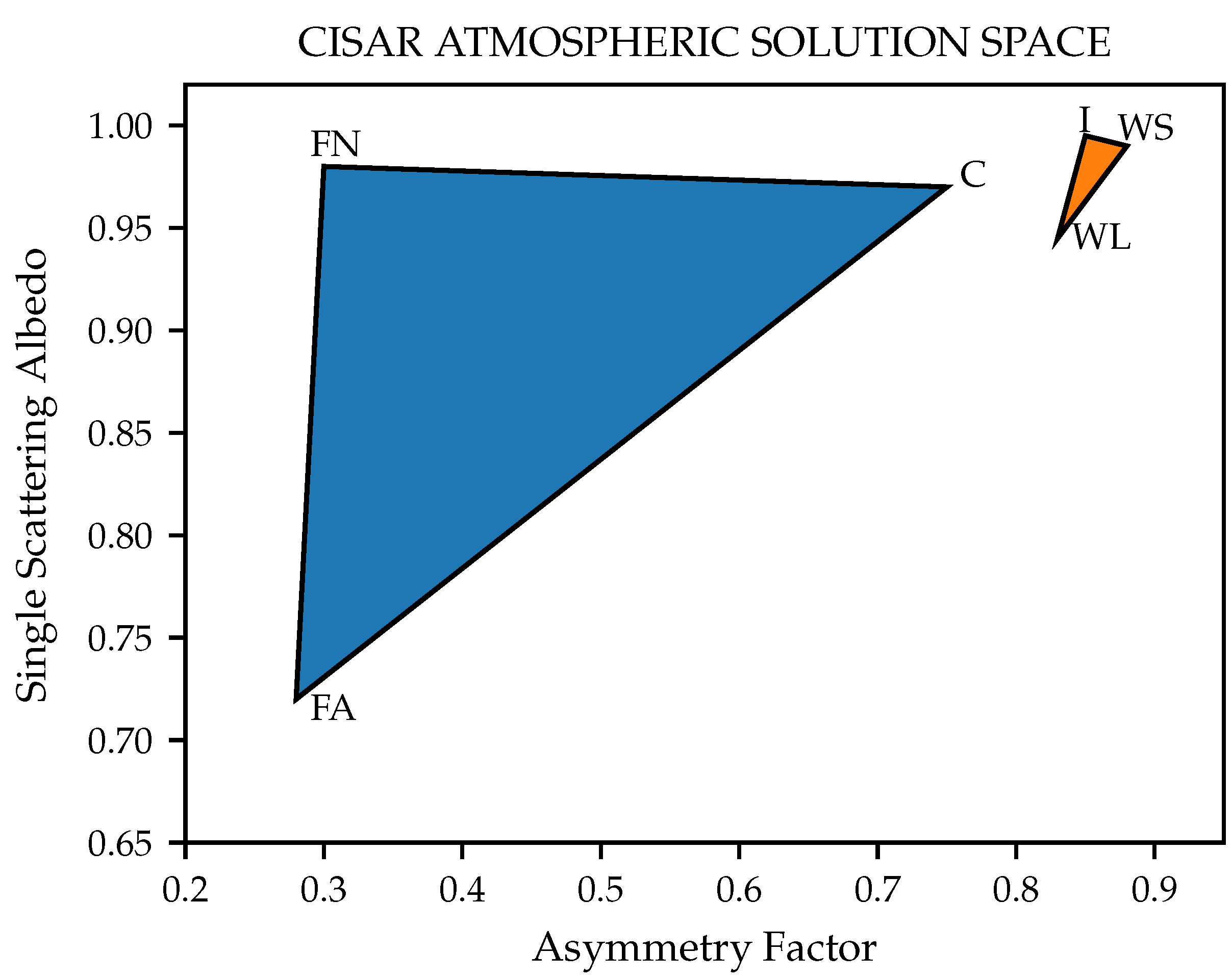
2.2.1. CISAR Atmospheric Solution Space

The CISAR aerosol properties solution space is defined as the portion of the two-dimensional single scattering albedo ($\omega$) and asymmetry factor (g) space delimited by three selected aerosol vertices. The latter represent absorbing and non-absorbing fine mode and coarse mode particles [17]. The inversion process retrieves the AOT associated with each vertex. The asymmetry factor and the single scattering albedo are then calculated as a mean of the properties associated with the three vertices weighted by the retrieved optical thickness:

$$\begin{array}{c}\hfill {\omega }_{T_A}={\displaystyle \frac{{\tau }_{FN}{\omega }_{FN}+{\tau }_{FA}{\omega }_{FA}+{\tau }_C{\omega }_C}{{\tau }_{FN}+{\tau }_{FA}+{\tau }_C}}\\ \hfill g_{T_A}={\displaystyle \frac{{\tau }_{FN}{g}_{FN}+{\tau }_{FA}{g}_{FA}+{\tau }_C{g}_C}{{\tau }_{FN}+{\tau }_{FA}+{\tau }_C}}\end{array}$$

(1)

To extend the retrieval to cloud single scattering properties, three cloud vertices are defined to sample a different portion of the $\omega$-g space (Figure 1). The selected vertices represent small and large liquid and ice particles. The cloud single scattering properties are calculated similarly, as in Equation (2):

$$\begin{array}{c}\hfill {\omega }_{T_C}={\displaystyle \frac{{\tau }_{WL}{\omega }_{WL}+{\tau }_{WS}{\omega }_{WS}+{\tau }_I{\omega }_I}{{\tau }_{WL}+{\tau }_{WS}+{\tau }_I}}\\ \hfill g_{T_C}={\displaystyle \frac{{\tau }_{WL}{g}_{WL}+{\tau }_{WS}{g}_{WS}+{\tau }_I{g}_I}{{\tau }_{WL}+{\tau }_{WS}+{\tau }_I}}\end{array}$$

(2)

Nevertheless, the forward model used within CISAR, FASTRE, only has one scattering layer: this prevents the determination of the position of the aerosol layer with respect to the clouds. It is stressed here that the retrieval of cloud single scattering properties is considered a bypass product, and the main focus of the CISAR algorithm remains the retrieval of aerosol particles.

2.2.2. Prior Information

Within CISAR, the inversion is performed in an OE framework, which seeks the best balance between the information coming from the observation and the prior information, which consists of any additional knowledge on the observed scene. Constraints are applied to the surface reflectance and AOT magnitude, as well as to the temporal and spectral variability of the state variables. The latter is now applied to the cloud single scattering properties as well, helping the discrimination between aerosols and clouds. The new version of the algorithm requires an additional source of prior information associated with the cloud optical thickness (COT). Besides the prior information already discussed in [18], new features are introduced for the prior information on the aerosol and cloud properties and on the surface reflectance.

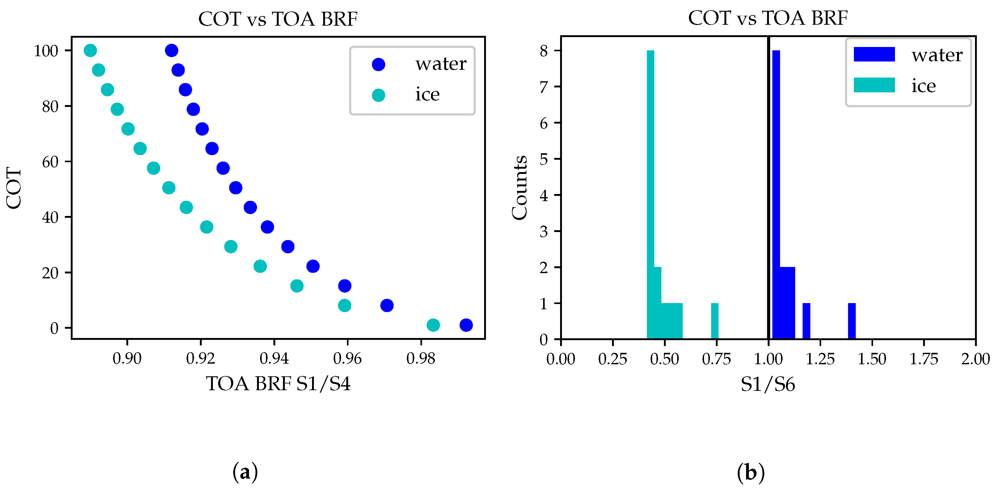
Cloud Phase and Optical Thickness

To develop meaningful prior information on the COT, the spectral signature of clouds has been simulated in the relevant part of the spectrum through the Radiation Transfer Matrix Operator Model (RTMOM, [22]), for which accuracy has been extensively documented [23]. Simulations have been made considering a wide range of particle size, compositions, and COT values. Figure 2 shows partial results of the RTMOM simulations for liquid (blue) and ice (cyan) clouds. The TOA BRF magnitude increases with the COT, although it tends to saturate for high values of COT. These results suggest that it is possible to build suitable prior information analyzing the spectral behavior of clouds in the spectral bands of the radiometer being processed. When applied to SLSTR data, the prior information on the cloud optical thickness is built considering the ratio between the TOA BRF in band S1 and the one in band S4. Figure 3 shows the values that this ratio takes for the above-mentioned RTMOM simulations. Given the evolution of the curves in Figure 3a, the prior information on the cloud COT is built as in Equation (3):

$${\widehat{x}}_{{\tau }_{cloud}}=1.4\times exp\left(35.0\times {\displaystyle \frac{{y_0}_{S4}}{{y_0}_{S1}}}\right),$$

(3)

where ${\widehat{x}}_{{\tau }_{cloud}}$ is the magnitude of the prior on the total COT and ${y_0}_{S1,S4}$ the TOA BRF in SLSTR bands S1 and S4 respectively.

The cloud phase discrimination can thus be built considering the ratio between the TOA BRF in bands S6 and S1: ice clouds are brighter at shorter wavelengths and darker in band S6, whereas liquid water clouds show opposite behavior (Figure 3b).

Spatial Constraints on AOT

One of the main technical advantages of the CISAR algorithm implementation is the ability to perform the inversion at the pixel level, meaning that the inversion of a pixel is fully independent. This allows a full parallelization of the code at a core level, as each pixel can be processed on a dedicated core independently from any surrounding pixel. While preserving this feature, spatial smoothing has been implemented, as aerosols are supposed to have a slow spatial variability in a few tenths of kilometers of the spatial window. This is achieved by exploiting the temporal overlap between two successive accumulation periods (see Section 2.2) and using the solution retrieved in the first period to build the prior information in the second. In particular, for each solution retrieved during the period $P_i$ at pixel p, a weighted mean is computed over the surrounding $N_p\times N_p$ pixels, accounting for the distance from the central pixel, and used as prior information for the same pixel at the period $P_{i+1}$. The value of $N_p$ is chosen according to the spatial resolution. Within this study, $N_P$ is set equal to 3, which corresponds to a 30 × 30 km window.

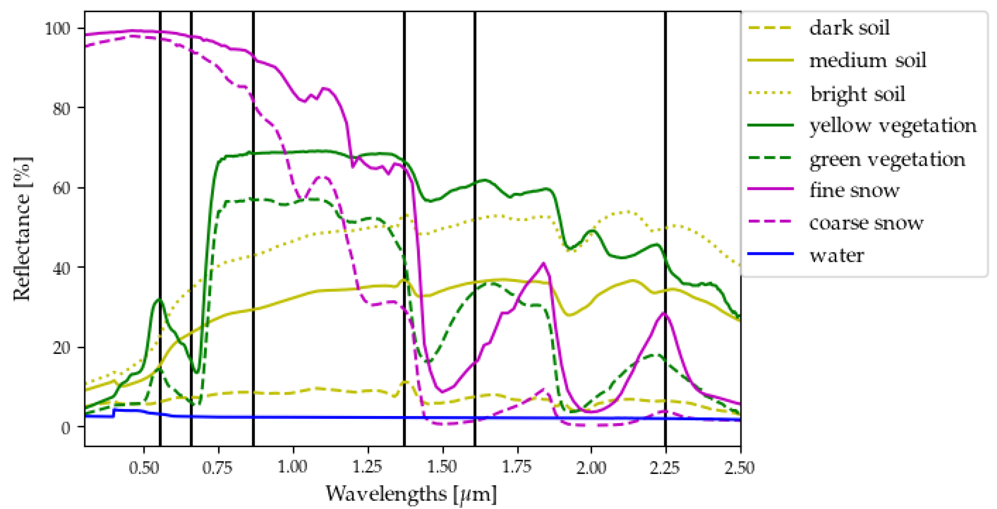
Surface Parameters Climatology

The retrieval of the surface reflectance is strongly complicated in cloudy conditions. The accurate retrieval of the surface reflectance is, however, necessary for the correct retrieval of atmospheric properties for a physically-based algorithm such as CISAR, taking into account the radiative coupling between the surface and the atmosphere. To maintain the ability to correctly retrieve the surface reflectance, and, thus, correctly account for the radiative coupling between surface and atmosphere, the CISAR prior information on the surface parameters has been improved by analyzing the MODIS/MAIAC MCD19A3 product [24]. A new Rahman–Pinty–Verstraete (RPV, [25]) global climatology is prepared by averaging the MODIS RossThick/Li-Sparse (RTLS, [26]) parameters during 10 years (2010–2020) over the four seasons and converting them to RPV parameters in the SLSTR bands. The new climatology is used as default prior information on the four RPV surface parameters at the very first accumulation period. For the successive accumulation periods, the prior is updated, as explained in [18]. The new climatology is also analyzed and used to define spectral constraints on the surface model parameters in the sensor bands. In the case of SLSTR, a strong spectral relation in the magnitude of the reflectance is found between bands S1–S2 and S5–S6. These spectral constraints are considered valid for any type of land cover except for snow coverage, where the surface reflectance shows a very different spectral signature, with large values at shorter wavelengths (Figure 4). For this reason, snow pixels are currently disregarded by the processing. Snow coverage is identified by computing the normalized-difference snow index (NDSI) from bands S1 and S6 [27]. Pixels showing an NDSI larger than 0.75 are classified as snow and discarded by the processing. The implementation of the surface spectral constraints has a large positive impact on the retrieval of the surface reflectance, as it improves the discrimination between cloud and surface contribution. A future version of the CISAR algorithm will include different spectral constraints to be activated in case of snow coverage.

2.3. Inversion

2.3.1. SLSTR Data Accumulation

S3A/SLSTR satellite images are accumulated during an accumulation period of 16 days (see Section 2.2) to build a multi-angular observation vector [18]. The accumulation periods are shifted by 12 days. The shift has been chosen in order to maximize the performances in terms of processing time while keeping an overlap between two consecutive periods where the spatial constraints discussed in Section 2.2.2 are applied. The availability of different acquisition geometries strongly impacts the information content of the observations [28]. The SLSTR dual view, however, introduces a clear difference between the Northern and Southern Hemispheres, as the oblique view is always observing in the backward scattering direction for latitude above about 20${}^{°}$ south [29]. This particular feature is quantitatively analyzed in Figure 5. The polar plot shows how Lindenberg, located in the Northern Hemisphere (Figure 5a), is always observed in the backward scattering configuration, while this is not the case for Bandung, located in the Southern Hemisphere (Figure 5b). The information content associated with aerosols is limited in the backward scattering direction, as aerosol particles mostly scatter in the forward direction, given the positive sign of the asymmetry factor g [30]. The time series in Figure 5 show that as the $cosg$ (cosine of the scattering angle) approaches zero and negative values, the Jacobian (i.e., the partial derivative of the TOA BRF with respect to the state variable) associated with the aerosol optical thickness decreases. In Figure 5, the large difference in the information content between the two hemispheres, quantified by the magnitude of the Jacobian, is visible. Given the above considerations, CISAR is expected to show better aerosol retrieval performances in the Southern Hemisphere.

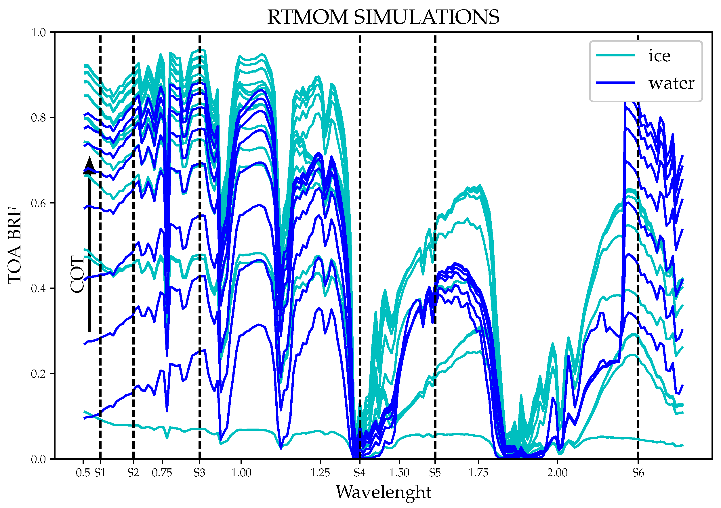
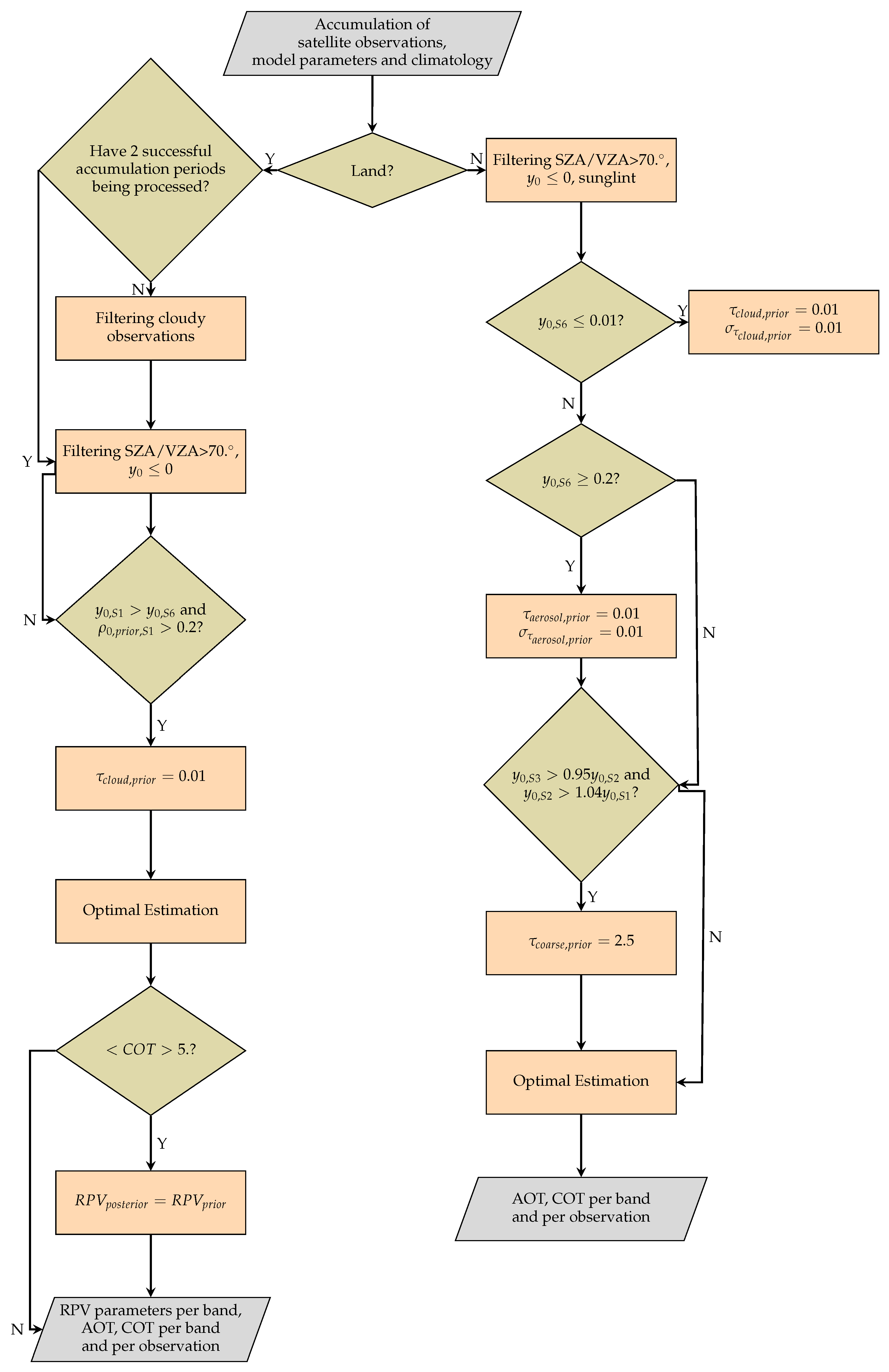
2.3.2. Data Processing

The SLSTR observations, accumulated as described in Section 2.3.1, together with all the necessary ancillary information (surface pressure, wind speed, total column water vapor, total column ozone, aerosol layer height), are inverted by the CISAR algorithm. The processing of cloudy observations implies new challenges with respect to algorithms retrieving only aerosol properties. The data filtering, the preparation of the prior information, and the data processing are slightly different for water and land pixels. The description of the method applied to the pixels according to their land cover type is described in the following paragraphs and summarized in the flowchart in Figure 6.

Processing over Land

One of the main issues associated with the processing of clouds with the CISAR algorithm is that the surface is not visible under thick clouds. Figure 7 shows the magnitude of the Jacobian associated with the four RPV parameters with respect to the retrieved COT. These results are obtained from the processing of one year of data over 16 AERONET stations with different locations and land cover. It can be seen that the Jacobians rapidly converge towards 0 as the COT increases. To address this issue, the CISAR algorithm is first trained with two cloud-free accumulation periods before discarding the use of the preprocessed cloud mask. In this way, the surface reflectance retrieved in the first two cloud-free accumulation periods is used to build strong prior information for the next periods, where no cloud mask is applied to classify the satellite observations. This so-called memory mechanism is explained in detail in [18]. However, it must be noted that mostly cloudy accumulation periods are still likely to happen. In order to not compromise the prior information on the surface with cloud-contaminated information, the RPV parameters are set equal to the prior information when the average retrieved COT within the accumulation period is larger than five. In other words, no surface reflectance retrieval is taking place when the average COT during the whole accumulation period exceeds five.

In addition, aerosol and cloud retrieval is particularly challenging over bright soil, where the signal from the surface is dominant [31]. However, both the aerosol and the cloud contributions are lower at 2.2 $\mathsf{\mu }$m than in the lower part of the visible spectrum, whereas the surface reflectance of bright soil increases with the wavelength. CISAR exploits this feature by setting a very low prior on the magnitude of the COT (equal to ${10}^{-2}$) when the TOA BRF in band S1 is larger than the one in band S6 and the retrieved ${\rho }_0$ surface parameter, which controls the magnitude of the surface reflectance, is larger than 0.2 in band S1.

Processing over Water

Cloud masking over water is generally less problematic than over land and it is often based on thresholds at wavelengths in the NIR spectral region [32]. However, high-aerosol events with larger particles, such as dust storms over the ocean, can be sometimes flagged as clouds by a threshold-based cloud masking algorithm. Within CISAR, three situations are defined based on the TOA BRF in band S6:

1.

Clear sky if TOA BRF in band S6 lower than 0.01;

2.

Cloudy if TOA BRF in band S6 larger than 0.2;

3.

Undefined otherwise.

If a pixel is flagged as cloud-free (cloudy), then the prior on the COT (AOT) is set to ${10}^{-2}$ with equal uncertainty. If a pixel falls in the undefined case, the prior for the aerosol and cloud classes is prepared as in Section 2.2.2. One exception to the above-mentioned cases is thick dust plumes over water. As dust and clouds have very similar spectral signatures, dust storms are often misclassified as clouds by many cloud-masking algorithms [33]. However, dust and clouds show some differences in the visible bands (S1, S2, and S3 in the case of SLSTR), which make clouds appear as white and thick dust brown-ish in a false-color composite image (see Figure 8 and in Video S1 in the Supplementary Materials) [34]. In particular, if $y_{0,S3}>0.95y_{0,S2}$ and $y_{0,S2}>1.04y_{0,S1}$, then a pixel is flagged as dust and the prior information on the AOT associated with the coarse mode is set to 2.5.

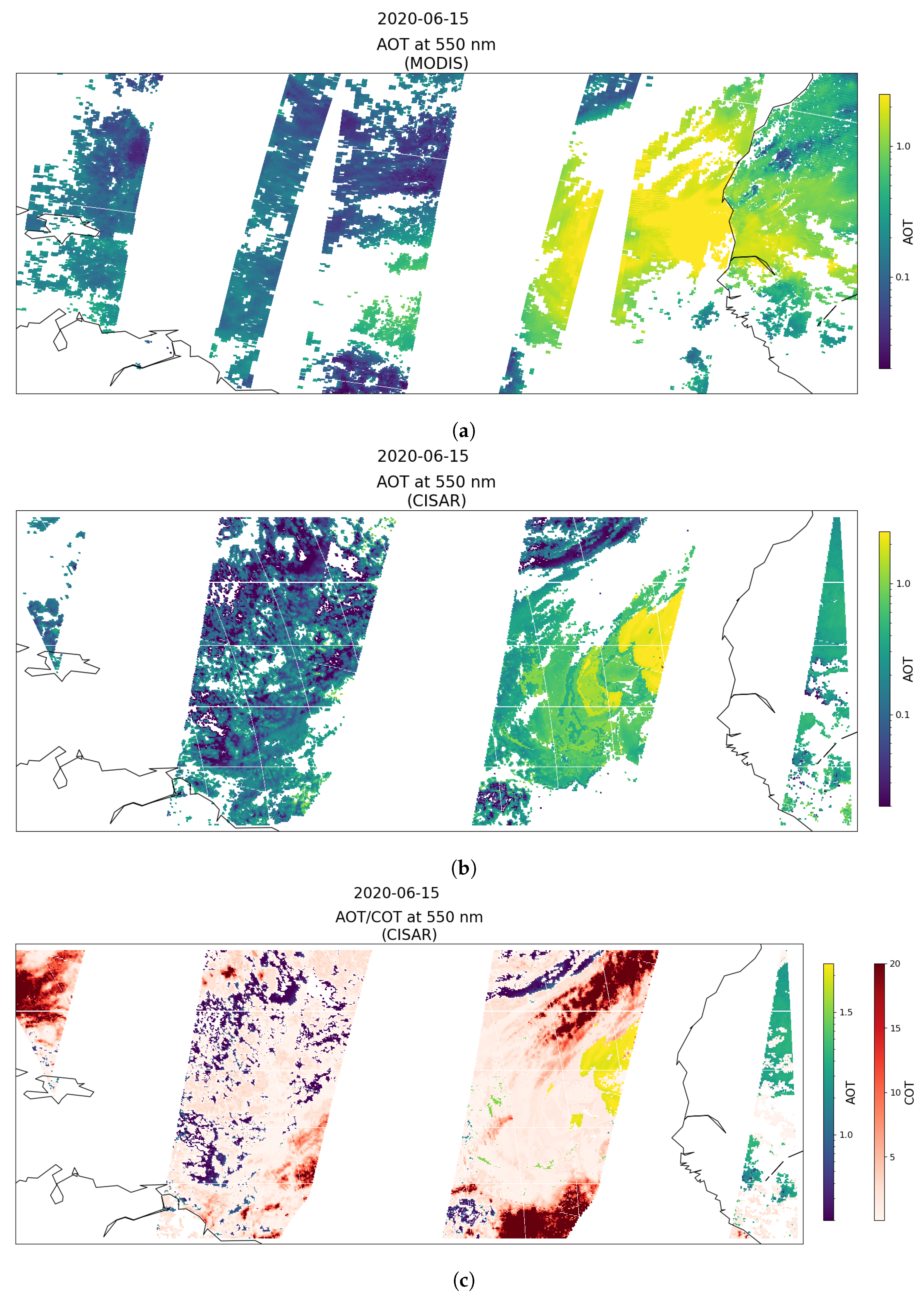
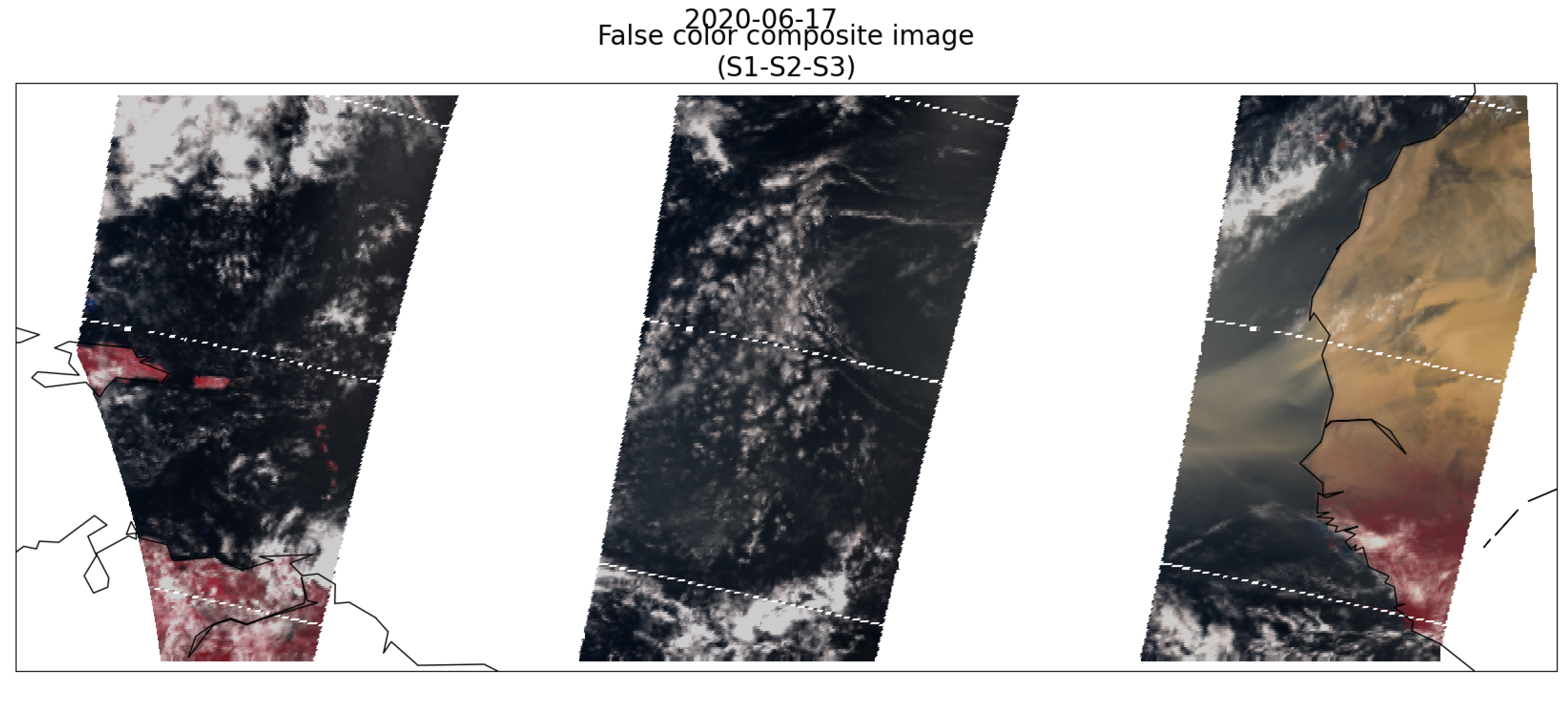
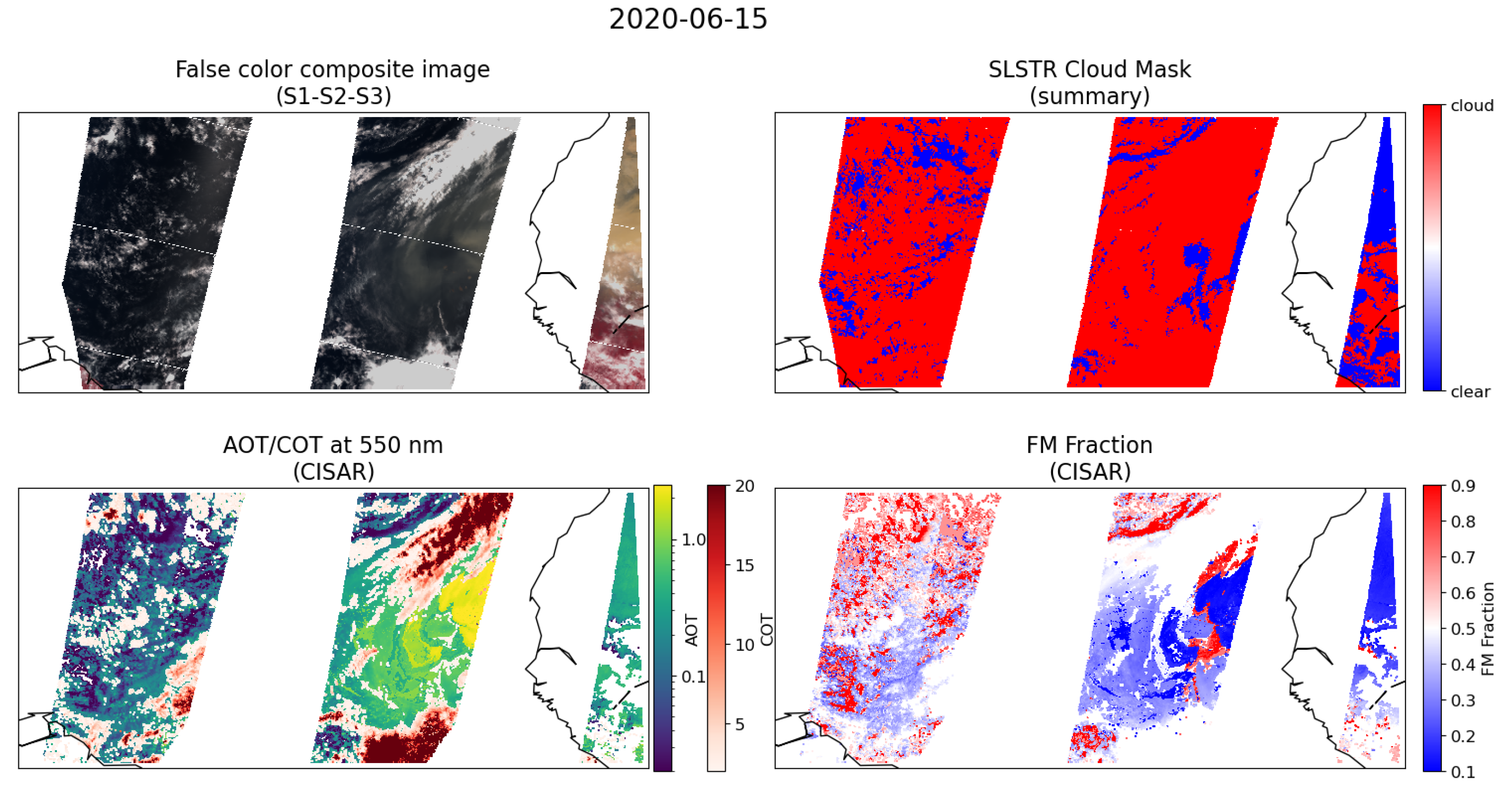
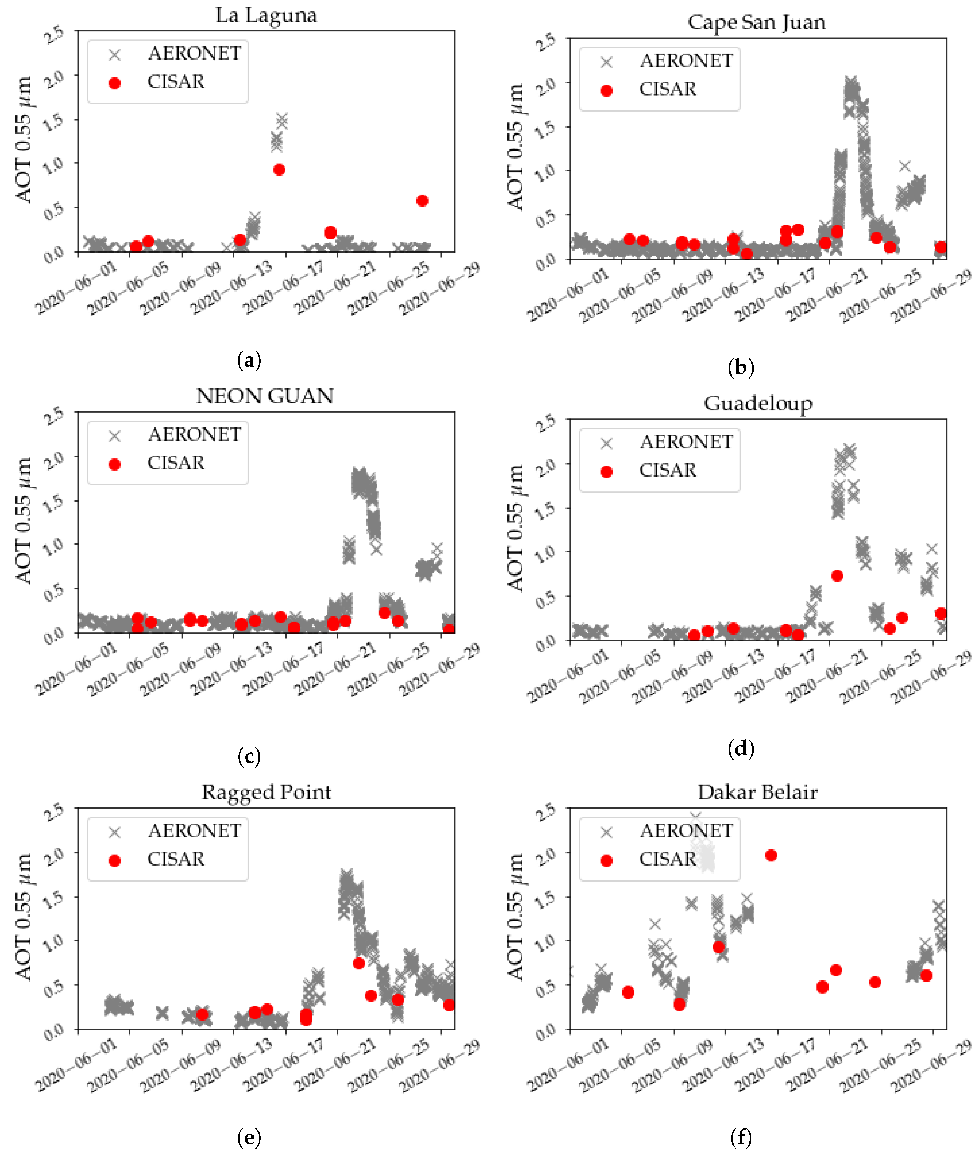
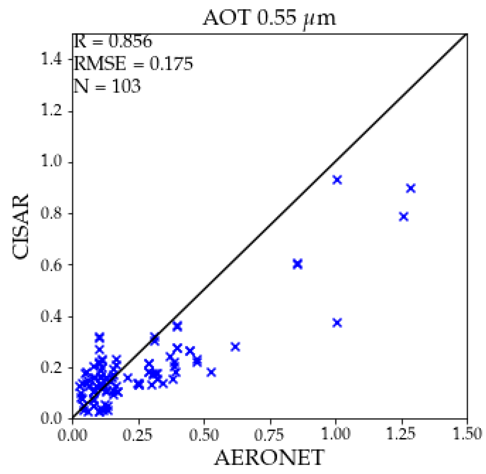
3. Case Study: The Godzilla Dust Storm

Sand and dust storms are extreme and rapidly evolving meteorological phenomena that generate significant amounts of mineral particles in the atmosphere. Desert dust represents a major portion of the global aerosol burden [35] and plays an important role in Earth’s radiative balance [36]. The Sahara desert is the world’s first source of dust, accounting for 40–70% of the global amount of dust in the atmosphere [37]. Unfortunately, dust storms observed by satellite remote sensing are often misclassified as clouds, as the spectral signature of dust is very similar to the one of clouds [33]. Every year, Saharan dust is transported towards the Caribbean islands; this phenomenon reaches its maximum during the summer months [38]. In particular, in June 2020, a dust plume originating from Sahara was transported towards the Caribbean islands, traveling more than 8000 km and peaking between 14 and 20 June. This dust storm was so extreme that it has been named Godzilla. This extraordinary dust plume, nearly as big as the continental United States, weighed almost 24 million tons. Godzilla was surprising not only in terms of size and weight but also in terms of its trigger. Typically, the dust storms are driven by warm, moist air from monsoons on the southern edge of the Sahara that blows to the north; Godzilla, on the other hand, was triggered by a large patch of high-pressure air parked over the northwestern edge of Africa [39]. Starting from 14 June, strong winds blowing at more than 70 km/h transported the dust storm, lifting it up to 6 km into the atmosphere, which is higher than the 5 km for the climatological summertime extreme dust events [40]. The Godzilla dust storm was partially predicted by climate models such as the Copernicus Atmosphere Monitoring Service (CAMS) [41]. However, time series of the predicted AOT from CAMS reanalysis show some underestimation of high values of AOT with respect to AERONET.

Most of the dust storm is unfortunately misclassified as cloud from the SLSTR summary cloud flag (see Figure 9). Aerosol retrieval algorithms only inverting clear-sky observations would therefore completely miss such an exceptional event. Conversely, the CISAR algorithm, not relying on an external cloud mask, performs the retrieval over all SLSTR observations regardless of the cloud mask classification. Figure 9 shows the false-color composite obtained from SLSTR bands S1, S2, and S3, the SLSTR summary cloud flag, the combined AOT and COT retrieval at $0.55$ $\mathsf{\mu }\mathrm{m}$ with the CISAR algorithm, and the FM fraction associated with the AOT retrieval. It can be seen that most of the dust storm, partially visible in the false-color composite, is flagged as cloud. In particular, about 85% of SLSTR observations in Figure 9 are flagged as cloud; with a retrieval algorithm only inverting clear-sky observations, the aerosol retrieval would be performed only on the remaining 15% of the pixels. CISAR, however, retrieves valid AOT (i.e., greater than 0) over 35% of all SLSTR observations, greatly improving the spatial coverage of the AOT product.

Finally, the thick dust plume visible in the false-color composite is correctly retrieved as coarse mode by CISAR, as seen in the bottom right panel in Figure 9 and in Video S2 in the Supplementary Materials. From the animation, it can be seen that the thick Godzilla dust plume is retrieved as coarse mode (FM fraction close to 0), although the fine-coarse mode discrimination is less accurate as the dust plume becomes optically thinner (around the 20 June). The retrieval of the FM fraction from the CISAR algorithm is qualitatively compared with the MODIS/Terra aerosol product MOD04 L2 v6.1 [42] in Figure 10. Both products retrieve the dust plume visible in the false-color composite in the top left panel in Figure 9 as coarse mode, while a higher fraction of FM is observed close to clouds. CISAR also retrieved some FM aerosols around the thick dust plume, although this is not observed in the MODIS product. From the Supplementary Materials, an increase in the FM fraction close to clouds can also be observed, similar to what was observed by [43], analyzing MODIS images and AERONET products. Ref. [43] found that the high AOT close to cloud edges exhibits high-frequency variability, possibly resulting from the turbulent environment in the immediate vicinity of convective cells.

Despite not exploiting any external cloud mask, CISAR is also capable of correctly retrieving the position of both thick and thin clouds close to the African western coast, visible in the red color scale in Figure 9, where only COT retrievals higher than two are shown to better observe the AOT retrieval. However, CISAR retrieves a low cloud optical thickness (COT < 2) within a few kilometers away from the clouds. Ref. [44] showed that cloud contamination can be observed within 15 km away from the clouds; with its ability to retrieve both AOT and COT within the same pixels, CISAR not only improves the aerosol product spatial coverage but also addresses the issue of cloud contamination from nearby clouds without the need of a safety zone. On the other hand, CISAR’s tendency to also retrieve a small COT a few kilometers away from clouds could result in a slight underestimation of the AOT, due to a not-optimal aerosol/cloud discrimination.

Video S1 in the Supplementary Materials shows the temporal evolution of the Godzilla dust storm as observed by the CISAR algorithm, together with the false-color composite from SLSTR bands S1, S2, and S3. During the time series, it can be seen that CISAR correctly follows the spatial and temporal variability of the dust storm originating close to the African coast around 14 June 2020 and being transported over the Atlantic ocean. Godzilla reaches the Caribbean islands on 21 June, with a CISAR-retrieved AOT of about 1. During the time series in Video S1 in the Supplementary Materials, it can be seen how CISAR correctly retrieves the position of clouds, solely relying on the SLSTR observations and the prior information built from the TOA BRF spectral signature with respect to the clouds one, without any external cloud masking operation. It is also possible to visually observe the effect of the sensor dual view on CISAR retrieval. As seen in Section 2.3.1, most of the information content is carried by the oblique view, leading to differences in the CISAR retrieval when only observations acquired in the nadir view are available. This leads to sharp discontinuities in the CISAR product, such as during 20 June over the Atlantic ocean.

Figure 11 evaluates the retrieval of the AOT at $0.55$ $\mathsf{\mu }\mathrm{m}$ against AERONET observations. It can be seen that CISAR correctly retrieves the temporal evolution of the aerosol load during June 2020, although unfortunately, no SLSTR observations were available over Cape San Juan and NEON GUAN when Godzilla reached these stations. It should also be stressed here that in this exercise, point measurements from the AERONET stations are being compared with satellite retrievals at 10 km. It is therefore expected that some discrepancies between the two datasets will be observed, as the dust storm moves quickly and its thickness can vary within a few kilometers [45]. Despite some underestimation which could be partially explained by the different spatial resolutions, CISAR correctly retrieves the increase in the aerosol load both close to the African coast (La Laguna, Dakar) and the Caribbean islands (Ragged Point, Guadeloupe). At the same time, CISAR correctly retrieves low values of AOT during the days not affected by the Godzilla storm, in good agreement with AERONET. Figure 12 shows the scatterplot between the AOT at $0.55$ $\mathsf{\mu }\mathrm{m}$ as delivered by CISAR and the AERONET dataset over the six stations listed in Figure 11. Only CISAR retrievals showing a quality indicator (QI) larger than 0 are shown in Figure 12 [18]. The resulting correlation between CISAR and AERONET is as high as 0.856.

Finally, CISAR AOT retrieval has been compared with the MODIS/Terra aerosol product MOD04 L2 v6.1 [42]. Terra overpassing local time is 10:30 a.m., while S3/SLSTR acquires observations at 10 a.m. local time. Both AOT products retrieve very high AOT (larger than 2) at the western African coast, although different spatial features can be observed (Figure 13). CISAR correctly retrieves the shape of the tick dust plume, also partially visible in Figure 9 (top left panel), but around it, CISAR also retrieves low values of COT. This leads to sharp borders of the dust plume and lower retrieved AOT values than in the MODIS product. Results in Figure 13 show that although CISAR can correctly retrieve high aerosol load spatial and temporal evolution, the discrimination between aerosol and thin cloud could further improve. CISAR retrieval shows slightly higher spatial coverage (especially closer to South America) as the retrieval is extended near clouds as well as within thin clouds; because of the extended spatial coverage, it is possible to observe the changes in AOT near clouds, as discussed in Section 1 [12].

4. Discussion

This paper describes an innovative approach to aerosol retrieval, where surface reflectance, aerosol, and cloud single scattering properties are retrieved consistently with the same RTM, without relying on any external cloud mask. The goal of this approach is to remove an external cloud mask, given the strong dependency of aerosol retrieval to the masking algorithm and the number of issues linked to lost pixels and cloud contamination [3,4,5,9].

The new version of the CISAR algorithm has been applied to S3A/SLSTR observations during June 2020 over the Atlantic Ocean, when an exceptionally large dust storm event originating from the Sahara region was transported by thousands of kilometers towards the Caribbean islands. This extreme dust plume, renamed Godzilla, was mostly misclassified as cloud by the SLSTR summary cloud mask. On 15 June, algorithms only inverting cloud-free observations would have performed the retrieval only over 15% of all available SLSTR observations. CISAR AOT retrieval, however, is valid (AOT larger than 0) over more than 35% of the total number of pixels, improving the spatial coverage by a factor of 2.3.

When evaluated against the AERONET dataset, the AOT retrieved by CISAR shows good agreement both in terms of magnitude and temporal evolution, with a correlation higher than 0.8 (see Figure 12). CISAR proves capable to retrieve both very low AOT in Figure 11, away from the Godzilla dust storm, and values larger than 1.0 when the pixel is affected by the dust. Comparison against the MOD04 v6.1 MODIS product in Figure 13 shows that although CISAR correctly identified the high aerosol load, it tends to underestimate it with respect to MODIS, as a low value of COT (lower than two) is also retrieved within the same pixel by the CISAR algorithm. This results in the total optical thickness being in good agreement with the MODIS product, but differently distributed between the aerosols and clouds. Compared to the MODIS MOD04 v6.1, the CISAR retrievals extend to near clouds, where the increased AOT due to the aerosol particle swelling caused by more hydration can be seen. In addition, the Godzilla dust storm is correctly identified as coarse mode by the CISAR algorithm, although the fine-coarse mode discrimination degrades as the AOT decreases, as shown in Video S2 in the Supplementary Materials of the fine mode fraction during the second half of June 2020, available in the Supplementary Materials. Overall, the evaluation of the CISAR aerosol retrieval against AERONET and MODIS products shows encouraging results. Furthermore, despite the main focus of the retrieval of the remaining aerosol single scattering properties, CISAR is capable of correctly identifying clouds without relying on any external preprocessing algorithm. The magnitude of the retrieved COT is also consistent with the false-color composite obtained from SLSTR observations. The cloud product retrieved by CISAR could be more extensively studied and validated in future work.

Results in Section 3 confirm the possibility of approaching aerosol retrieval in an innovative way, overcoming the need for an external cloud mask with all the issues associated with it (lost pixels, cloud contamination, etc.). The uniqueness of such a continuous product between clouds and aerosols represents a powerful tool for better studying and understanding the aerosol properties in the vicinity of clouds. Several recent studies suggest that performing the retrieval of aerosol particles only in clear-sky conditions could lead to a significant negative underestimation in the aerosol direct radiative effect [16]. The CISAR product, extending the aerosol retrieval in the vicinity and within thin clouds, could be exploited to more extensively study aerosol properties far from clear-sky conditions, as suggested by [14,15].

The proposed approach still has some limitations. The quality of the CISAR retrieval depends on the information content associated with the satellite observations; in the case of SLSTR, this is visible in the sharp edges in the AOT product at the overlap between the oblique and nadir view (Section 3), where the amount of information is strongly reduced due to the observation geometry, as seen in Section 2.3.1. In addition, the discrimination between aerosols and thin clouds is not always successful, as discussed in Section 3. The current implementation of the spectral constraints on the surface reflectance excludes snow pixels from the retrieval. A continuous effort is made to address these limitations and further improve the CISAR algorithm. Finally, being based on the inversion of a 1D radiative transfer model, any 3D effects between clouds and clear-sky pixels cannot be correctly characterized with the CISAR algorithm.

The proposed ambitious method paves the way for an innovative and critical approach to aerosol retrieval, aiming at deepening the knowledge of aerosols in the vicinity of clouds by delivering a continuous aerosol–cloud product. To achieve such an ambitious objective, the CISAR algorithm solution space has been extended to clouds. By being able to retrieve both aerosol and cloud single scattering properties, CISAR is no longer dependent on a preprocessing cloud identification. By appropriate choice of the prior information and associated uncertainty on all the state variables, CISAR can retrieve the state of the observed system through the optimal estimation (OE) approach. With such an innovative product, not only is the spatial coverage of the aerosol product improved, but it is also possible to analyze the effect of aerosol swelling near clouds and the cloud-induced changes in their optical properties [13].

References

1. Stocker, T.; Qin, D.; Plattner, G.K.; Tignor, M.; Allen, S.; Boschung, J.; Nauels, A.; Xia, Y.; Bex, V.; Midgley, P. Climate Change 2013: The Physical Science Basis. In Contribution of Working Group I to the Fifth Assessment Report of the Intergovernmental Panel on Climate Change; Cambridge University Press: Cambridge, UK, 2013. [Google Scholar]
2. WHO. Ambient (Outdoor) Air Pollution; WHO: Geneva, Switzerland, 2021. [Google Scholar]
3. Holzer-Popp, T.; de Leeuw, G.; Griesfeller, J.; Martynenko, D.; Klüser, L.; Bevan, S.; Davies, W.; Ducos, F.; Deuzé, J.L.; Graigner, R.G.; et al. Aerosol retrieval experiments in the ESA Aerosol_cci project. Atmos. Meas. Tech. 2013, 6, 1919–1957. [Google Scholar] [CrossRef] [Green Version]
4. Remer, L.A.; Mattoo, S.; Levy, R.C.; Heidinger, A.; Pierce, R.B.; Chin, M. Retrieving aerosol in a cloudy environment: Aerosol product availability as a function of spatial resolution. Atmos. Meas. Tech. 2012, 5, 1823–1840. [Google Scholar] [CrossRef] [Green Version]
5. Koren, I.; Remer, L.A.; Kaufman, Y.J.; Rudich, Y.; Martins, J.V. On the twilight zone between clouds and aerosols. Geophys. Res. Lett. 2007, 34. [Google Scholar] [CrossRef] [Green Version]
6. Marshak, A.; Wen, G.; Coakley, J.A., Jr.; Remer, L.A.; Loeb, N.G.; Cahalan, R.F. A simple model for the cloud adjacency effect and the apparent bluing of aerosols near clouds. J. Geophys. Res. Atmos. 2008, 113. [Google Scholar] [CrossRef] [Green Version]
7. Várnai, T.; Marshak, A. MODIS observations of enhanced clear sky reflectance near clouds. Geophys. Res. Lett. 2009, 36, L06807. [Google Scholar] [CrossRef]
8. Chand, D.; Wood, R.; Ghan, S.J.; Wang, M.; Ovchinnikov, M.; Rasch, P.J.; Miller, S.; Schichtel, B.; Moore, T. Aerosol optical depth increase in partly cloudy conditions. J. Geophys. Res. Atmos. 2012, 117. [Google Scholar] [CrossRef]
9. Schwarz, K.; Cermak, J.; Fuchs, J.; Andersen, H. Mapping the Twilight Zone—What We Are Missing between Clouds and Aerosols. Remote Sens. 2017, 9, 577. [Google Scholar] [CrossRef] [Green Version]
10. Kassianov, E.I.; Ovtchinnikov, M. On reflectance ratios and aerosol optical depth retrieval in the presence of cumulus clouds. Geophys. Res. Lett. 2008, 35. [Google Scholar] [CrossRef]
11. Poulsen, C.A.; Siddans, R.; Thomas, G.E.; Sayer, A.M.; Grainger, R.G.; Campmany, E.; Dean, S.M.; Arnold, C.; Watts, P.D. Cloud retrievals from satellite data using optimal estimation: Evaluation and application to ATSR. Atmos. Meas. Tech. 2012, 5, 1889–1910. [Google Scholar] [CrossRef] [Green Version]
12. Quaas, J.; Stevens, B.; Stier, P.; Lohmann, U. Interpreting the cloud cover—aerosol optical depth relationship found in satellite data using a general circulation model. Atmos. Chem. Phys. 2010, 10, 6129–6135. [Google Scholar] [CrossRef] [Green Version]
13. Spencer, R.S.; Levy, R.C.; Remer, L.A.; Mattoo, S.; Arnold, G.T.; Hlavka, D.L.; Meyer, K.G.; Marshak, A.; Wilcox, E.M.; Platnick, S.E. Exploring Aerosols Near Clouds with High-Spatial-Resolution Aircraft Remote Sensing During SEAC4RS. J. Geophys. Res. Atmos. 2019, 124, 2148–2173. [Google Scholar] [CrossRef]
14. Rosenfeld, D.; Sherwood, S.; Wood, R.; Donner, L. Climate Effects of Aerosol-Cloud Interactions. Science 2014, 343, 379–380. [Google Scholar] [CrossRef] [PubMed]
15. Seinfeld, J.H.; Bretherton, C.; Carslaw, K.S.; Coe, H.; DeMott, P.J.; Dunlea, E.J.; Feingold, G.; Ghan, S.; Guenther, A.B.; Kahn, R.; et al. Improving our fundamental understanding of the role of aerosol-cloud interactions in the climate system. Proc. Natl. Acad. Sci. USA 2016, 113, 5781–5790. [Google Scholar] [CrossRef] [PubMed] [Green Version]
16. Marshak, A.; Ackerman, A.; Da Silva, A.; Eck, T.; Holben, B.; Kahn, R.; Kleidman, R.; Knobelspiesse, K.; Levy, R.; Lyapustin, A.; et al. Aerosol Properties in Cloudy Environments from Remote Sensing Observations: A Review of the Current State of Knowledge. Bull. Am. Meteorol. Soc. 2021, 102, E2177–E2197. [Google Scholar] [CrossRef]
17. Govaerts, Y.; Luffarelli, M. Joint retrieval of surface reflectance and aerosol properties with continuous variation of the state variables in the solution space—Part 1: Theoretical concept. Atmos. Meas. Tech. 2018, 11, 6589–6603. [Google Scholar] [CrossRef]
18. Luffarelli, M.; Govaerts, Y. Joint retrieval of surface reflectance and aerosol properties with continuous variation of the state variables in the solution space—Part 2: Application to geostationary and polar-orbiting satellite observations. Atmos. Meas. Tech. 2019, 12, 791–809. [Google Scholar] [CrossRef] [Green Version]
19. Smith, D.L. Lessons Learned from (A)ATSR and Prelaunch Calibration of SLSTR; Technical Report; RAL Space: Didcot, UK, 2013. [Google Scholar]
20. De Leeuw, G.; Holzer-Popp, T.; Bevan, S.; Davies, W.H.; Descloitres, J.; Grainger, R.G.; Griesfeller, J.; Heckel, A.; Kinne, S.; Klüser, L.; et al. Evaluation of seven European aerosol optical depth retrieval algorithms for climate analysis. Remote Sens. Environ. 2015, 162, 295–315. [Google Scholar] [CrossRef] [Green Version]
21. Jethva, H.; Torres, O.; Yoshida, Y. Accuracy assessment of MODIS land aerosol optical thickness algorithms using AERONET measurements over North America. Atmos. Meas. Tech. 2019, 12, 4291–4307. [Google Scholar] [CrossRef] [Green Version]
22. Govaerts, Y. RTMOM V0B.10 User’s Manual; Technical Report; EUMETSAT: Darmstadt, Germany, 2006. [Google Scholar]
23. Govaerts, Y. RTMOM V0B.10 Evaluation Report; Technical Report; EUMETSAT: Darmstadt, Germany, 2006. [Google Scholar]
24. Lyapustin, A.; Wang, Y. Mcd19a3 MODIS/Terra+Aqua BRDF Model Parameters 8-Day L3 Global 1 km SIN Grid v006; Technical Report; LP DAAC: Sioux Falls, SD, USA, 2018. [Google Scholar]
25. Rahman, H.; Pinty, B.; Verstraete, M.M. Coupled surface-atmosphere reflectance (CSAR) model. 2. Semiempirical surface model usable with NOAA Advanced Very High Resolution Radiometer Data. J. Geophys. Res. 1993, 98, 20791–20801. [Google Scholar] [CrossRef]
26. Lucht, W.; Schaaf, C.; Strahler, A. An algorithm for the retrieval of albedo from space using semiempirical BRDF models. IEEE Trans. Geosci. Remote Sens. 2000, 38, 977–998. [Google Scholar] [CrossRef] [Green Version]
27. Hall, D.K.; Riggs, G.A. Normalized-Difference Snow Index (NDSI). In Encyclopedia of Snow, Ice and Glaciers; Singh, V.P., Haritashya, U.K., Eds.; Springer: Dordrecht, The Netherlands, 2011; pp. 779–780. [Google Scholar] [CrossRef] [Green Version]
28. Luffarelli, M.; Govaerts, Y.; Damman, A. Assessing Hourly Aerosol Property Retrieval from MSG/SEVIRI Observations in the Framework of Aerosol_CCI2; ESA: Paris, France, 2016. [Google Scholar]
29. EUMETSAT. Copernicus Sentinel-3 NRT Aerosol Optical Depth; EUMETSAT: Darmstadt, Germany, 2020. [Google Scholar]
30. Andrews, E.; Sheridan, P.J.; Fiebig, M.; McComiskey, A.; Ogren, J.A.; Arnott, P.; Covert, D.; Elleman, R.; Gasparini, R.; Collins, D.; et al. Comparison of methods for deriving aerosol asymmetry parameter. J. Geophys. Res. Atmos. 2006, 111. [Google Scholar] [CrossRef] [Green Version]
31. Hsu, N.; Tsay, S.C.; King, M.; Herman, J. Aerosol properties over bright-reflecting source regions. IEEE Trans. Geosci. Remote Sens. 2004, 42, 557–569. [Google Scholar] [CrossRef]
32. Wang, M.; Shi, W. Cloud Masking for Ocean Color Data Processing in the Coastal Regions. IEEE Trans. Geosci. Remote Sens. 2006, 44, 3105–3196. [Google Scholar] [CrossRef]
33. Liu, J.; Chen, B.; Huang, J. Discrimination and validation of clouds and dust aerosol layers over the Sahara Desert with combined CALIOP and IIR measurements. J. Meteorol. Res. 2014, 28, 185–198. [Google Scholar] [CrossRef]
34. Zhou, Y.; Levy, R.C.; Remer, L.A.; Mattoo, S.; Shi, Y.; Wang, C. Dust Aerosol Retrieval over the Oceans with the MODIS/VIIRS Dark-Target Algorithm: 1. Dust Detection. Earth Space Sci. 2020, 7, e2020EA001221. [Google Scholar] [CrossRef]
35. Monks, P.S.; Granier, C.; Fuzzi, S.; Stohl, A.; Williams, M.L.; Akimoto, H.; Amann, M.; Baklanov, A.; Baltensperger, U.; Bey, I.; et al. Atmospheric composition change—Global and regional air quality. Atmos. Environ. 2009, 43, 5268–5350. [Google Scholar] [CrossRef] [Green Version]
36. Weinzierl, B.; Ansmann, A.; Prospero, J.M.; Althausen, D.; Benker, N.; Chouza, F.; Dollner, M.; Farrell, D.; Fomba, W.K.; Freudenthaler, V.; et al. The Saharan Aerosol Long-Range Transport and Aerosol–Cloud-Interaction Experiment: Overview and Selected Highlights. Bull. Am. Meteorol. Soc. 2017, 98, 1427–1451. [Google Scholar] [CrossRef] [Green Version]
37. Engelstaedter, S.; Tegen, I.; Washington, R. North African dust emissions and transport. Earth-Sci. Rev. 2006, 79, 73–100. [Google Scholar] [CrossRef]
38. Petit, R.H. Transport of Saharan dust over the Caribbean Islands: Study of an event. J. Geophys. Res. 2005, 110, D18S09. [Google Scholar] [CrossRef]
39. Cornwall, W. ‘Godzilla’ dust storm traced to shaky northern jet stream. Science 2020. [Google Scholar] [CrossRef]
40. Huang, J.; Zhang, C.; Prospero, J.M. African dust outbreaks: A satellite perspective of temporal and spatial variability over the tropical Atlantic Ocean. J. Geophys. Res. Atmos. 2010, 115. [Google Scholar] [CrossRef] [Green Version]
41. Errera, Q.; Bennouna, Y.; Schulz, M.; Eskes, H.; Basart, S.; Benedictow, A.; Blechschmidt, A.M.; Chabrillat, S.; Clark, H.; Cuevas, E.; et al. Validation Report of the CAMS Global Reanalysis of Aerosols and Reactive Gases, Years 2003–2020; Copernicus Atmosphere Monitoring Service: Brussels, Belgium, 2021. [Google Scholar] [CrossRef]
42. Levy, R.; Hsu, C. MODIS Atmosphere L2 Aerosol Product. NASA MODIS Adaptive Processing System; Goddard Space Flight Center: Greenbelt, MD, USA, 2015. [Google Scholar] [CrossRef]
43. Eck, T.F.; Holben, B.N.; Reid, J.S.; Arola, A.; Ferrare, R.A.; Hostetler, C.A.; Crumeyrolle, S.N.; Berkoff, T.A.; Welton, E.J.; Lolli, S.; et al. Observations of rapid aerosol optical depth enhancements in the vicinity of polluted cumulus clouds. Atmos. Chem. Phys. 2014, 14, 11633–11656. [Google Scholar] [CrossRef] [Green Version]
44. Christensen, M.W.; Neubauer, D.; Poulsen, C.A.; Thomas, G.E.; McGarragh, R.; Povey, A.C.; Proud, S.R.; Grainger, R.G. Unveiling aerosol-cloud interactions Part 1: Cloud contamination in satellite products enhances the aerosol indirect forcing estimate. Atmos. Chem. Phys. 2017, 17, 13151–13164. [Google Scholar] [CrossRef] [Green Version]
45. Jiang, X.; Liu, Y.; Yu, B.; Jiang, M. Comparison of MISR aerosol optical thickness with AERONET measurements in Beijing metropolitan area. Remote Sens. Environ. 2007, 107, 45–53. [Google Scholar] [CrossRef]
Figure 1. Example of the CISAR solution space for aerosol and cloud single scattering properties. The x-axis represents the asymmetry factor and the y axis represents the single scattering albedo. The blue triangle represents the solution space for the aerosol particles, delimited by the three vertices associated with fine absorbing (FA), fine non-absorbing (FN), and coarse (C) mode particles. The orange triangle is the solution space in which the cloud properties are allowed to change, delimited by the vertices representing small and large water (WS and WL, respectively) and ice (I) particles.
Atmosphere 13 00691 g001
Figure 2. Results from the RTMOM simulations on ice (cyan) and liquid (blue) particle of different radius, with associated cloud optical thickness (COT) varying from 1 to 80. The dashed vertical lines represent the central wavelengths of the S3A/SLSTR bands from S1 to S6.
Atmosphere 13 00691 g002
Figure 3. (a) The plot of the simulated COT values (y axis) with respect to the ratio between the top-of-atmosphere (TOA) bidirectional reflectance factor (BRF) in band S1 and S4 (x axis) for both ice (cyan) and liquid (blue) clouds. (b) The histogram of the distribution of the ratio between the TOA BRF in bands S1 and S6. The color code follows from Figure 2. It can been seen that the ratio is always larger than one (S1 brighter than S6) for ice clouds, while the opposite is true for water clouds.
Atmosphere 13 00691 g003
Figure 4. Representative spectral reflectance of snow, clouds, soil, and vegetation in the visible and infrared range.
Atmosphere 13 00691 g004
Figure 5. The polar plots (a) show the acquisition geometry over Lindenberg, Germany (52.209 ° N, 14.121 ° E) and Bandung, Australia (6.888 ° S, 107.610 ° E). The orange diamonds represent the solar angles, blue symbols represent the viewing angles. Circles represent the zenith angle and polar angles represent azimuth angles with zero azimuth pointing to the north. (b) The time series of the aerosol optical thickness (AOT) Jacobians (blue, left axis) and the cosine of the scattering angle (brown, right axis) from March 2017 to March 2018. Dots and crosses represent the nadir and oblique views, respectively.
Atmosphere 13 00691 g005
Figure 6. Flowchart of CISAR inversion of one accumulation period.
Atmosphere 13 00691 g006
Figure 7. Magnitude of the Jacobian associated with each parameter of the Rahman–Pinty–Verstraete (RPV) surface model in function of the CISAR-retrieved COT. Given the different order of magnitude among the Jacobians, two scales are here used to better visualize the Jacobian dependency on the COT. The right y-axis is related to the ρ 0 , associated with the surface reflectance magnitude; the left y-axis is related to k (representing the bell or bowl shape of the surface anisotropy), θ (describing the presence of forward or backward scattering), and ρ c (associated with the hot spot effect), associated with the surface reflectance shape.
Atmosphere 13 00691 g007
Figure 8. False-color composite obtained from SLSTR bands S1, S2, and S3 over the Atlantic Ocean during 17 June 2020. A thick dust plume is visible at the western coast of Africa.
Atmosphere 13 00691 g008
Figure 9. (Top left panel): false-color composite obtained from SLSTR bands S1, S2, and S3. (Top right panel): SLSTR summary cloud mask, where blue indicates clear sky and red indicates cloud. (Bottom left panel): combined AOT/COT retrieval at 0.55 μ m with the CISAR algorithm. Only COT > 2 is shown. (Bottom right panel): Fine mode (FM) fraction associated with the CISAR aerosol retrieval.
Atmosphere 13 00691 g009
Figure 10. FM fraction associated to the CISAR (a) and MODIS (b) aerosol retrieval.
Atmosphere 13 00691 g010
Figure 11. AOT timeseries over six AERONET stations (La Laguna (a), Cape San Juan (b)), NEON GUAN (c), Guadeloup (d), Ragged Point (e), and Dakar Belair (f) affected by the Godzilla dust storm.
Atmosphere 13 00691 g011
Figure 12. Scatterplot between the AOT at 0.55 μ m retrieved by CISAR (y axis) and delivered by the AERONET V3 L2 product (x axis). Correlation (R), root mean square error (RMSE), and number of CISAR-AERONET collocations within a ±30 min window (N) are shown in the plot.
Atmosphere 13 00691 g012
Figure 13. AOT at 0.55 μ m as retrieved by the combined Dark Target and Deep Blue algorithms applied to MODIS/Terra (a) and by CISAR (b). (c) CISAR combined AOT/COT product for all COT retrievals larger than 0.1.
Atmosphere 13 00691 g013