Traveling 10-Day Waves at Mid-Latitudes in the Troposphere and Lower Stratosphere Revealed by Radiosonde Observations and MERRA-2 Data in 2020

Abstract

Although the characteristics of the traveling 10-day waves (10DWs) above the middle stratosphere have been well explored, little research has been performed on the counterpart in the troposphere and lower stratosphere (TLS). In the present study, we use radiosonde observations and MERRA-2 data from 2020 to characterize traveling 10DWs in mid-latitudes in the TLS. Single-site observations in both hemispheres show that strong 10DW activities are always accompanied by strong eastward jets (10–13 km). MERRA-2 data indicate that in the troposphere, the eastward-propagating modes with larger wavenumbers, i.e., E3, E4, E5 and E6 are dominant, while in the lower stratosphere, the eastward- and westward-propagating modes with small zonal wavenumbers, e.g., 1 and 2, are dominant. Further research on E3, E4, E5 and E6 modes in the troposphere of both hemispheres shows that all the wave activities are positively correlated to the background zonal wind. The refractive index squared reveals that a strong eastward jet is suitable for these four modes to propagate. However, just above the jet, the eastward wind decreases with altitude, and a thick evanescence region emerges above 15 km. E3, E4, E5 and E6 10DWs cannot propagate upward across the tropopause; as such, this can explain why these four modes are weak or even indiscernible in the stratosphere and above. In the troposphere, E5 10DW at 32° S was the most dominant mode in 2020. A case study of the anomalously strong E5 10DW activity on 12 May 2020 indicates that the wave amplification resulted from the upward and equatorward transmission of wave energy flows. Moreover, the tropopause and equatorial region can prevent the propagations of wave energy flows of E5 10DW. The upward-propagating wave energy is deposited near the tropopause, resulting in significant short-term variability in the tropopause height.

1. Introduction

Atmospheric waves, including planetary waves (PWs), gravity waves (GWs) and tides [1,2,3], are periodic disturbances of the atmosphere with respect to the mean background state; these disturbances are detected in the fields of atmospheric meteorological parameters, e.g., the wind velocity, temperature, geopotential height and pressure. Atmospheric waves dominate throughout the atmosphere and play pivotal roles in determining local and global atmospheric variations and transient structures [4,5,6]. PWs are large-scale atmospheric oscillations that can be divided into quasi-stationary PWs and traveling PWs [7,8], where the latter can be classified either as free modes or as forced waves. The free modes, also known as Rossby normal modes, can be obtained from the solutions of Laplace’s tidal equation [9]. A free mode is often expressed as ($s,n-s$), where s is the zonal wavenumber and n is the meridional index. The predicted periods of free modes include ∼2 days for the ($3,0$) mode, ∼4 days for the ($2,1$) mode, ∼5 days for the ($1,1$) mode, ∼7 days for the ($2,2$) mode, 10 days for the ($1,2$) mode, ∼16 days for the ($1,3$) mode and ∼28 days for the ($1,4$) mode [10]. The ($3,0$) mode, the ($1,1$) mode, the ($1,2$) mode and the ($1,3$) mode are often referred to as quasi-2-day wave (QTDW), quasi-5-day wave (Q5DW), quasi-10-day wave (Q10DW) and quasi-16-day wave (Q16DW), respectively [2]. Normal modes with these typical periods have been observed in the stratosphere, mesosphere and lower thermosphere [10,11,12,13,14] and have been the topic of theoretical investigations for many decades [2,7,9,14,15,16]. Interestingly, many scholars discovered that the actual wavefields associated with these quasi-periodic waves contain a number of other modes, e.g., the eastward-propagating modes and westward-propagating modes with zonal wavenumbers different from those of the abovementioned normal modes. These traveling modes also play key roles in and interact with other waves or the mean flow, thereby affecting atmospheric dynamics [12,13,17,18,19,20].

Compared with the research on other quasi-periodic PWs, investigations specifically considering traveling 10DWs have been relatively rare, and almost all of these studies were focused on the stratosphere and above. For instance, the normal mode of the 10DW was clearly observed in the global stratosphere by using satellite observations, which suggested that it always persisted for 1–2 months and was stronger in the Northern Hemisphere (NH) than in the Southern Hemisphere (SH) [15]. In addition, dominant 10DWs were detected in the mid-latitude lower ionosphere and were considered to be caused by PWs coming from below [21]. Ionospheric sounding data revealed that the F-layer electron density profiles were modulated by PW-type oscillations, e.g., modes with 2-day, 5-day, 10-day and 16-day periods [22]. As revealed by the Canadian Middle Atmosphere Model (CMAM), the normal mode of the 10DW is strongly correlated with variations in the chemical species between 30 and 60 km [23]. Moreover, PWs play an important role in ozone transport throughout the stratosphere. For instance, the 10DWs found in ozone profile data and medium-frequency radar (MFR) wind data were both consistent with the normal mode [24]. Sounding of the atmosphere using broadband emission radiometry (SABER) temperature measurements were employed to provide a comprehensive perspective of the westward-propagating 10DW with zonal wavenumber 1 between 20 and 100 km at latitudes of 50° S–50° N [14]. In the following, the westward-propagating and eastward-propagating modes with zonal wavenumber n are referred to as Wn and En, respectively, for simplicity. The W1, W2, E1 and E2 10DWs were studied in detail by using thermosphere, ionosphere, mesosphere, energetics and dynamics (TIMED) SABER observations, which are all strong at high latitudes during winter [18]. Moreover, the eastward-propagating 10DWs were found to be governed by different mechanisms from those responsible for the normal modes. Using the long-term modern era retrospective-analysis for research and applications version 2 (MERRA-2) database, Huang et al. [19] found that W1, E1 and E2 10DWs are the dominant traveling waves below the middle mesosphere, and reach their peaks near the stratopause. The E1 and E2 10DWs in the stratosphere might come from those downward-propagating waves excited in the mesosphere by the mean flow instability. Additionally, the enhanced PW activity in the middle atmosphere is a typical phenomenon during or after sudden stratospheric warming (SSW) [25]. Consequently, the association of 10DWs with SSW events has received some attention over the past two decades [17,20,26,27,28,29], with researchers finding that enhanced 10DWs are closely related to SSW. Ultimately, the abovementioned studies demonstrated that the 10DW field in the stratosphere and above is dominated by modes with small zonal wavenumbers, i.e., W1, W2, E1 and E2.

Nevertheless, PWs in the troposphere and lower stratosphere (TLS), the main source region of atmospheric waves, have not been adequately studied. Baroclinic instability, the forcing action of zonally asymmetric heating, and topography could all serve as sources of PWs in the troposphere [30]. It is worth noting that PWs in the TLS have greater wind amplitudes (usually larger than 10 ms⁻¹) than tides and GWs and thus deserve more attention [31,32,33]. As such, a few studies have involved the 10DWs in the TLS. As revealed by intensive radiosonde observations over Yichang (111°18′ E, 30°42′ N), 10DWs can exert great impacts on the tropospheric jet in winter and the tropopause in both summer and winter months and can obviously modulate diurnal tidal amplitudes [32]. The proximity of strong 10DWs near the tropospheric subtropical jet stream led some researchers to conclude that the jet stream strengthened the propagation of 10DWs and might even be their excitation source [34]. Huang et al. [35] studied the characteristics of PWs in the lower atmosphere over Xianghe (117.00° E, 39.77° N), China, by utilizing Beijing mesosphere–stratosphere–troposphere (MST) radar measurements and found 10DWs and 16DWs displaying similar seasonal and height variations, implying the same excitation source. In addition, these waves exhibited prevailing eastward propagation in the zonal direction and a quasi-standing structure in the vertical direction. These studies revealed some local characteristics of 10DWs in the TLS. From the perspective of their temporal and spatial resolutions and height coverage, radiosonde and MST radar data are quite suitable for studying local PWs in the TLS. However, the limitations of these data are obvious: the spatial distributions of radiosondes and MST radar stations are incredibly sparse, and the amount of observation data from these sources is still insufficient. Certainly, data from such a limited number of observation sites cannot provide accurate zonal wavenumber information for 10DWs. Moreover, the above studies revealed the characteristics of 10DWs in the TLS of only the NH. Accordingly, a number of unsolved questions remain, including the following: (1) What modes does the 10DW wavefield in the TLS contain? (2) Which mode of 10DWs is the dominant mode in the TLS? (3) Where and what are the sources of the 10DWs in the TLS? (4) What are the similarities and differences between the local characteristics of the 10DWs in the TLS, the NH and the SH?

To answer the above questions, we need not only local but also global observation data. Satellite observations with good altitude resolution are a good candidate. However, most satellites can provide high-precision observations only above the lower stratosphere [18]. MERRA-2 provides the latest atmospheric reanalysis data from the modern satellite era [36]. A variety of observations are assimilated in MERRA-2. As such, the database can provide relatively complete information on physical quantities such as horizontal wind and temperature in the TLS. In recent years, MERRA-2 data have been extensively used to reveal the global characteristics of atmospheric waves [19,27,29,37]. Hence, we dedicate this paper to addressing the above questions by combining radiosonde observations with MERRA-2 data.

In this paper, our main objective is to characterize the mid-latitude 10DWs in the TLS of both the NH and the SH from both local and global perspectives from 2020. After exposing the local characteristics of the complex 10DWs in both hemispheres by using radiosonde observations, we reveal the characteristics of the dominant modes of traveling 10DWs in the TLS of both hemispheres by leveraging MERRA-2 data. The datasets utilized in this paper are described in detail in the following section. The background zonal wind is presented in Section 3. Local 10DWs revealed by radiosonde observations are illustrated in Section 4. The dominant traveling 10-day modes are studied in Section 5. A case study of the most dominant mode in the SH is provided in Section 6. In the last section, we give a summary and the conclusions of our investigation.

2. Data Description

The integrated global radiosonde archive (IGRA) consists of radiosonde and pilot balloon observations from more than 2800 globally distributed stations. Until January 2018, IGRA provided atmospheric soundings, including pressure, temperature, humidity and wind measurements, at approximately 445 radiosonde sites across the globe. The sampling rate of a high-resolution radiosonde is 1 s or 2 s, which corresponds to a vertical resolution of approximately 5–10 m throughout the atmosphere. Synoptic radiosonde measurements are taken twice per day at 0000 and 1200 UTC [38]. We chose the radiosonde observations at Santa Teresa (106.7° W, 31.9° N) and Perth Airport (116.0° E, 31.9° S) to reveal the local characteristics of complex 10DWs in both hemispheres. The high-resolution radiosonde observations at Santa Teresa with a vertical resolution of 5 m are provided by the United States National Oceanic and Atmospheric Administration (NOAA). In addition, the University of Wyoming provides radiosonde observations at 93 high-resolution sites with a sampling rate of 1 s or 2 s, including the Perth Airport site. For convenience, the raw data are linearly interpolated to a uniform vertical resolution of 50 m.

MERRA-2 is the latest atmospheric reanalysis of the modern satellite era produced by the NASA Global Modeling and Assimilation Office (GMAO) [36]. The MERRA-2 product “inst6_3d_ana_Nv” used in the present study consists of reanalyzed fields at four synoptic times (00 GMT, 06 GMT, 12 GMT, and 18 GMT) at 72 nominal pressure levels varying from 985 hPa to 0.01 hPa with a native resolution of 0.625° longitude by 0.5° latitude. The product includes data spanning longitudes from 180.0° W to 179.375° E and latitudes from 90.0° S to 90.0° N. In this study, physical quantities of the eastward wind component (U), northward wind component (V) and air temperature (T) are considered for the analysis.

3. Background Mid-Latitude Zonal Wind in the TLS

PW activities are closely related to the background structure, especially the zonal-mean zonal wind. Before revealing the characteristics of the 10DWs at the two abovementioned radiosonde observation stations, we first present the background zonal winds at these two locations. To display the day-to-day variations in the background zonal wind, we adopt a sliding 30-day window with an increment of 1 day to extract the background zonal wind on the central date of each window. Then, the temporally averaged zonal wind within each window is regarded as the background component. Data loss does exist in the utilized radiosonde observations. Since more than 20 days of data are present in any 30-day window, the calculated background wind is reliable.

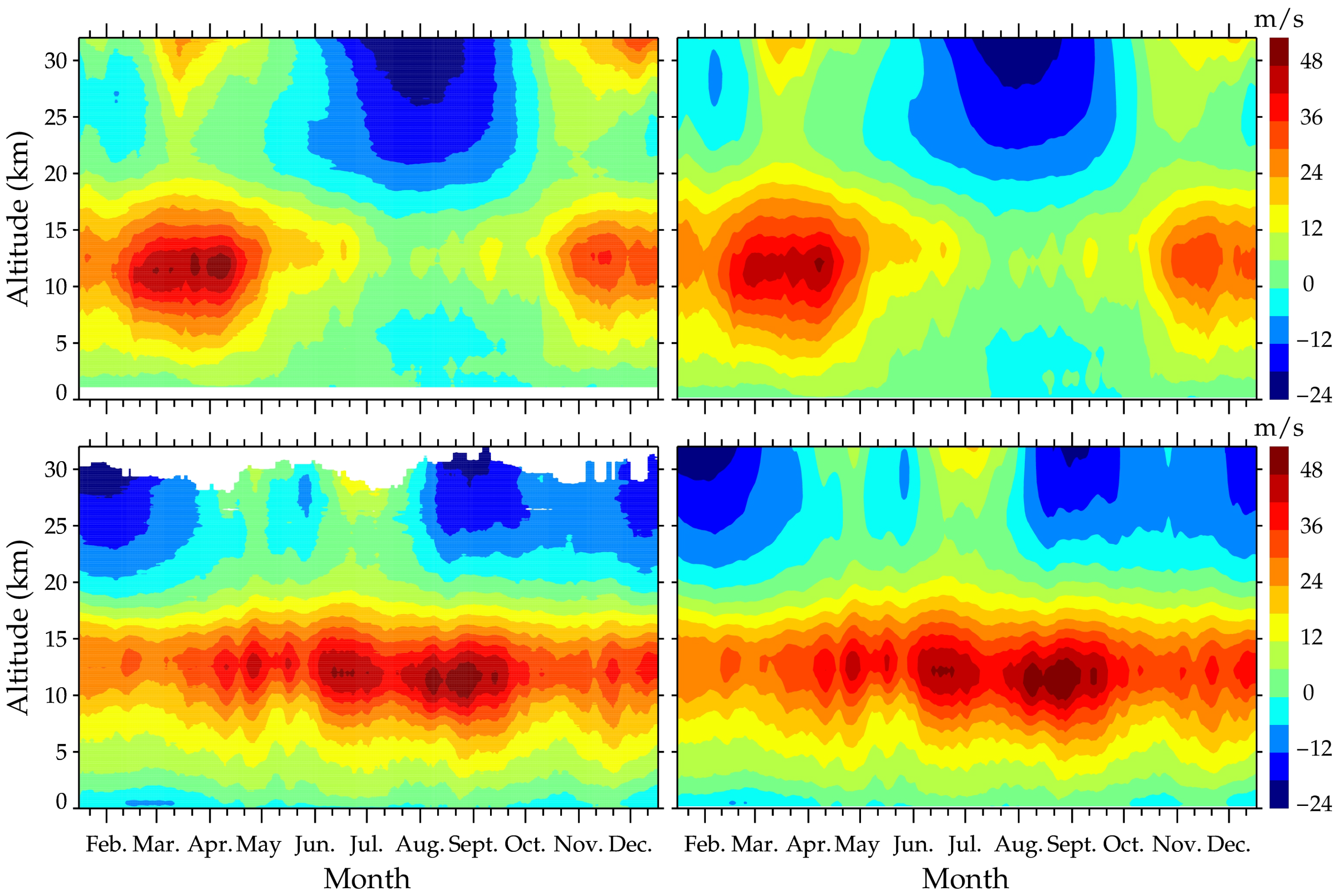
As visualized in the left panels of Figure 1, the background zonal winds at Santa Teresa and Perth Airport deduced from the radiosonde observations show characteristics that are highly similar to those revealed by previous observations at mid-latitudes [34,35]. In the troposphere, the background zonal wind manifests as a strong, predominantly eastward-propagating tropospheric jet at heights of approximately 10–13 km in spring and winter months in both hemispheres, reaching maximum values of 54.1 ms⁻¹ at 12.1 km in April at Santa Teresa and 54.5 ms⁻¹ at 11.9 km in August at Perth Airport. The zonal wind increases with altitude from 3.5 km up to approximately 12–13 km and then decreases with altitude. This is the typical tropospheric zonal wind structure at mid-latitudes. In the tropospheric jet stream area in summer and autumn, the eastward background zonal winds at Santa Teresa are evidently weaker than those at Perth Airport. In the lower stratosphere, the westward background zonal wind mainly appears in summer with maximum values of −24.1 ms⁻¹ at 32 km in July at Santa Teresa and −24.3 ms⁻¹ at 30.1 km in January at Perth Airport. Compared to its counterpart at Santa Teresa, the westward background zonal wind at Perth Airport persists over a longer time.

For comparison, the background zonal winds deduced from the MERRA-2 data at the two grid nodes nearest the observation stations ((106.875° W, 32° N) and (116.25° E, 32° S)) are also provided in the right panels of Figure 1. The background zonal winds deduced from the MERRA-2 data have similar spatial and temporal distributions to those deduced from the radiosonde observations. Nevertheless, slight differences are still observed.

4. Mid-Latitude Local 10DWs in the TLS

Previous studies revealed that PW-scale perturbations exist at the mid-latitudes in the TLS of the NH [32,34,35]. Radiosonde observations allow us to study PW-scale perturbations in the time domain. Accordingly, we performed a Lomb–Scargle periodogram analysis [39] to identify the primary oscillations.

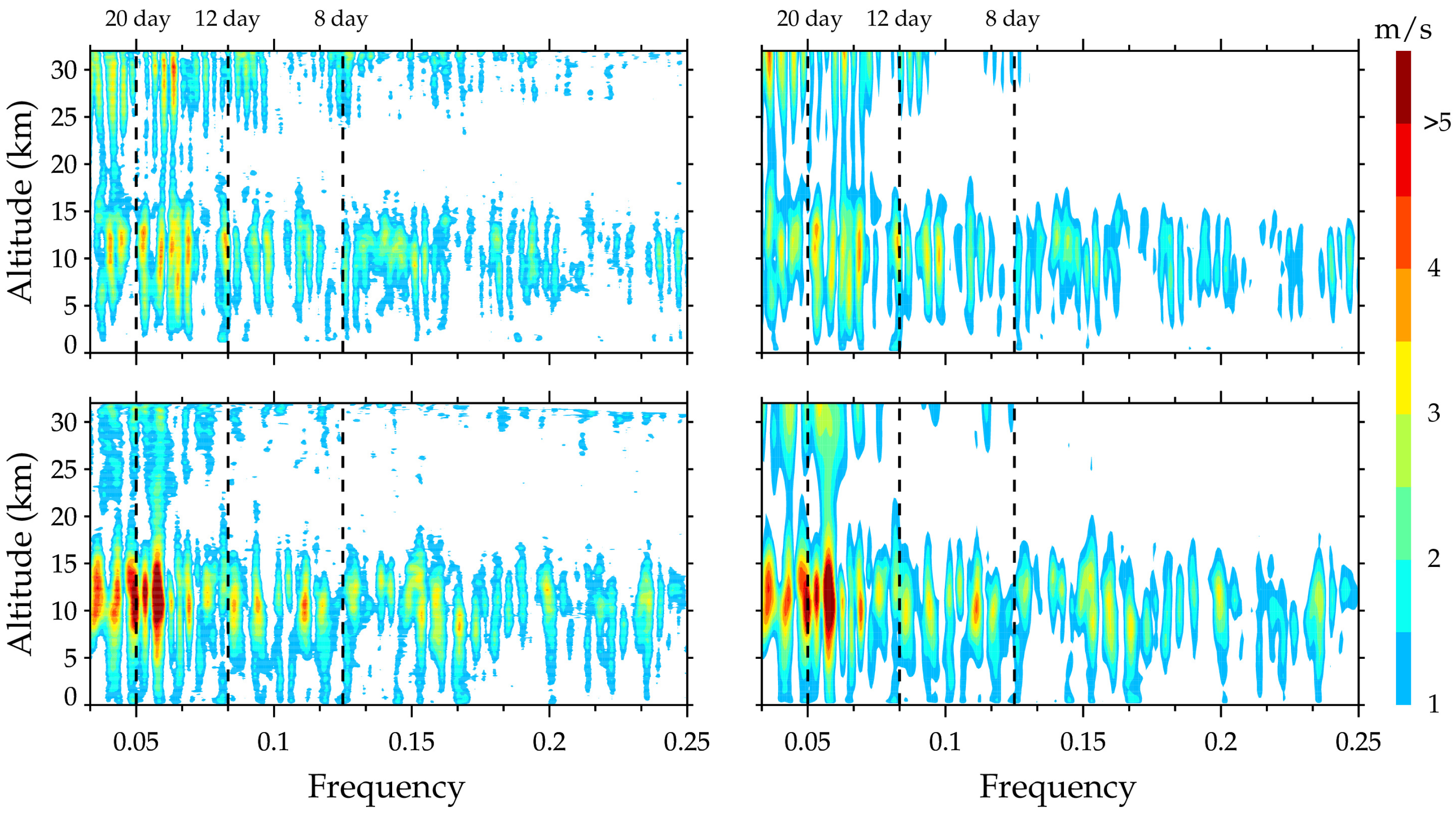
The frequency spectra of the zonal winds at each sampling height from the radiosonde observations at Santa Teresa and Perth Airport are plotted in the left panels of Figure 2 (only values greater than 1 ms⁻¹ are shown). At mid-latitudes in the TLS, three salient PW-scale perturbations are detected: the 16DW (12–20 days) [35], the 10DW (8–12 days) [14] and an oscillation with a period of approximately 20–30 days [40]. We aim to investigate 10DWs, which are not the strongest but are significant enough in this paper. However, the other oscillations might be within the scope of our future research. Significant 10DWs appear in two layers (5–15 km and 25–32 km), and these oscillations are stronger in the troposphere than in the lower stratosphere. At Santa Teresa, the strongest spectral peak of 3.2 ms⁻¹ is situated at ∼11 km with a period of 10.2 days; at Perth Airport, the strongest spectral peak of 4.2 ms⁻¹ is located at ∼11 km with a period of 9.1 days.

For comparison, the Lomb–Scargle periodograms of the zonal winds deduced from the MERRA-2 data at the same grid nodes as mentioned above are also provided in the right panels of Figure 2 and exhibit similar spatial and temporal distributions to those deduced from the radiosonde observations. However, slight differences are detected. For instance, the radiosonde observation-derived spectral magnitude with a period of 10.2 days at ∼11 km at Santa Teresa is slightly weaker than that derived from the MERRA-2 data. In addition, the radiosonde-derived spectra above 25 km at Perth Airport are slightly different from those obtained from the MERRA-2 data. In summary, we find significant 10DWs in the zonal winds.

The above Lomb–Scargle periodogram analysis shows that 10DWs exist in the zonal winds. To display the day-to-day variations in the 10DWs, we again adopt a sliding 30-day window with an increment of 1 day to extract the 10DWs on the central date of each window. Within each window, the time average and the linear trend are removed from the raw data as the background component. Then, the residuals are harmonically fitted within the period range from 8.0 to 12.0 days in increments of 0.5 days. Since 10DWs are quasiperiodic, they are classified using the period band from 8.0 to 12.0 days rather than a single period. The formula used for the fitting is as follows:

$$f^{\prime }\left(t\right)=Acos\left(\frac{2\pi }{T}t-\theta \right)$$

(1)

where t is the time in days, and A, T and $\theta$ are the amplitude, period and phase of the 10DWs, respectively. Since the utilized observation data contain time gaps, no fit is attempted if fewer than 18 days of data are present in a given 30-day window. The wave amplitude at any given height on the central date of each window corresponds to the one fit among these periods that has the largest amplitude. Moreover, because the data from a single sounding site cannot provide the zonal wavenumber information of 10DWs, the fitted amplitude corresponds to synthesized multimodal 10DWs, i.e., the superposition of multiple modes with different zonal wavenumbers.

The zonal wind amplitudes of the 10DWs deduced from the radiosonde observations at Santa Teresa and Perth Airport are provided in the left panels of Figure 3. Notable 10DWs appear in two layers (5–15 km and 25–32 km) at the mid-latitudes in the TLS in both hemispheres, which agrees well with the results from the Lomb–Scargle periodograms. Within the 5–15 km layer, strong wave activities appear in February (14 ms⁻¹), March (18 ms⁻¹), May (14 ms⁻¹), September (11 ms⁻¹), November (13 ms⁻¹), and December (12 ms⁻¹) at Santa Teresa and in January (12 ms⁻¹), March (12 ms⁻¹), April (18 ms⁻¹), May (19 ms⁻¹), June (19 ms⁻¹), July (16 ms⁻¹), August (16 ms⁻¹), September (14 ms⁻¹), October (17 ms⁻¹), November (11 ms⁻¹) and December (11 ms⁻¹) at Perth Airport. The waves at Santa Teresa are notable in spring, autumn and winter but weak in summer, and the strongest wave activity occurs in spring. Compared to their counterparts at Santa Teresa, the 10DWs at Perth Airport have slightly stronger amplitudes and more seasonal coverage. In particular, significant wave activities are observed even in summer, while the strongest wave activities take place in autumn and winter. The wave activities at 10–13 km are accompanied by strong eastward jets (Figure 1). Within the 25–32 km layer, strong 10DWs appear in January (18 ms⁻¹), March (18 ms⁻¹) and December (10 ms⁻¹) at Santa Teresa and in May (9 ms⁻¹), July (7 ms⁻¹) and August (9 ms⁻¹) at Perth Airport. Hence, in this layer, mid-latitude 10DWs with notable amplitudes exist at Santa Teresa during winter and spring and at Perth Airport during winter and autumn, and the 10DWs at Santa Teresa have a stronger amplitude than those at Perth Airport.

For comparison, the zonal winds of the 10DWs deduced from the MERRA-2 data at the same grid nodes as mentioned above are also provided in the right panels of Figure 3 and display very similar spatial and temporal distributions to those deduced from the radiosonde observations. However, subtle differences are still present. In particular, the radiosonde-derived 10DWs above 25 km in the NH are more intensive than those from the MERRA-2 data in January and March.

5. Dominant Modes of the Mid-Latitude 10DWs in the TLS

The 10DWs shown in the above section are the combination of multiple modes of 10DWs with different zonal wavenumbers. Some observational studies also confirmed these 10DWs in the troposphere of NH [32,34,35] but could not provide zonal wavenumber information because the applied observation data were from a single site. To reveal the dominant modes of those 10DWs, we use the MERRA-2 data along the same lines of latitude to calculate the frequency–wavenumber spectra by using a two-dimensional Fourier transform. The results in the above section demonstrate that the 10DWs are the strongest at ∼11 km in the troposphere and ∼31 km in the lower stratosphere, so we plot the frequency-wavenumber spectra at these two heights. To identify the prevailing modes of the 10DWs in 2020, a sliding 30-day window was adopted, this time with an increment of 10 days. Within each window, the time and zonal averages were removed from the raw data as the background component. Then, the frequency–wavenumber spectra were calculated for the residuals in each window. Throughout the whole year of 2020, there were 34 30-day windows in total, and then 34 frequency–wavenumber spectra are acquired. Finally, we arithmetically averaged all the 34 frequency-wavenumber spectra and normalized the average according to the maximum amplitude.

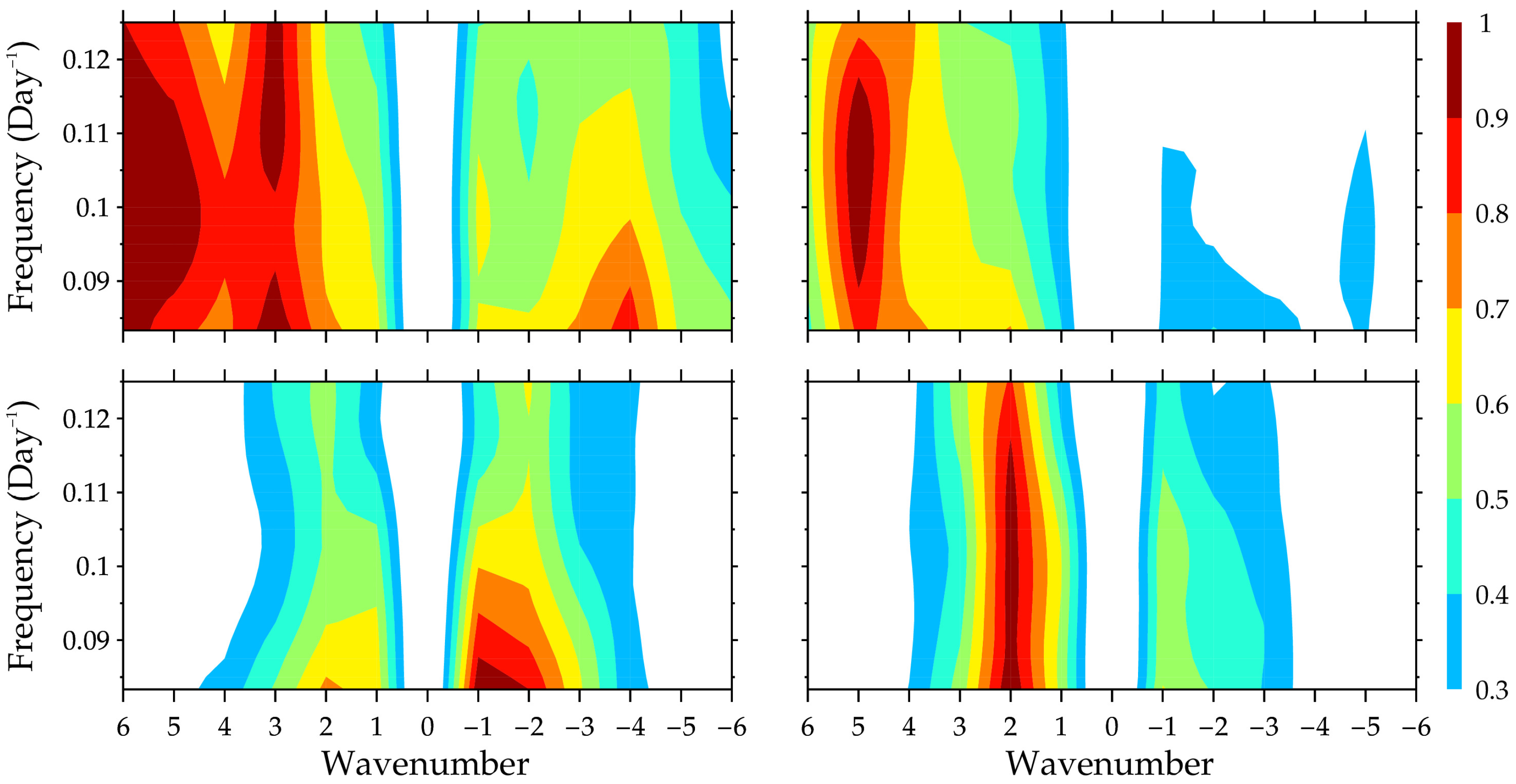
The normalized frequency-wavenumber spectra of the zonal wind disturbance at ∼11 km in 2020 are provided in the top row of Figure 4. The left panels show the results at 32° N, while the right panels show the results at 32° S. It should be noted that on the horizontal axis, positive zonal wavenumbers represent eastward propagation and negative zonal wavenumbers signify westward propagation. In the troposphere, the eastward-propagating modes are stronger than the westward-propagating modes. Among the eastward-propagating modes, those with larger wavenumbers are stronger than those with smaller wavenumbers. In the NH, E3 and E6 are almost as strong. In the SH, E5 is obviously stronger than the other modes. Likewise, the normalized frequency–wavenumber spectra of the zonal wind disturbance at ∼31 km in 2020 are provided in the bottom row of Figure 4. The left panels show the results at 32° N, while the right panels show the results at 32° S. Only the modes with small wavenumbers, e.g., 1 and 2, exist in the lower stratosphere. The strongest mode in the NH is W1, while the strongest mode in the SH is E2. We also checked the multi-year normalized frequency–wavenumber spectra for the 15 years from 2006 to 2020 (Figure not shown here), and similar conclusions were obtained.

The westward-propagating and eastward-propagating modes in the stratosphere and above with small wavenumbers, e.g., 1 and 2, were widely revealed by previous studies [14,15,18,19]. From here on, our study focuses only on the dominant modes in the troposphere that have received little attention. Figure 4 provides only the average intensity of each mode at ∼11 km in 2020. To reveal the temporal and spatial evolution characteristics of the eastward-propagating modes with large wavenumbers (E3–E6), the MERRA-2 data are harmonically fitted along the same lines of latitude using a sliding 30-day window with an increment of 1 day. Within each window, harmonic fits are performed on the residuals in the period range from 8.0 to 12.0 days in increments of 0.5 days. The formula used for the fitting is as follows:

$$f^{\prime }\left(\lambda ,t\right)=Acos\left(\frac{2\pi }{T}t-s\lambda -\theta \right)$$

(2)

where t, A, T and $\theta$ are the same quantities as in Equation (1). In addition, $\lambda$ is the longitude in radians, and s is the zonal wavenumber, where positive zonal wavenumbers represent eastward propagation and negative zonal wavenumbers signify westward propagation. For a certain mode of a 10-day wave, its amplitude at any given height in each window corresponds to the one fit among these periods that has the largest amplitude.

To ensure that the fitting result represents the actual signal rather than noise, we replace the zonal wind from the MERRA-2 data with values from a randomly generated Gaussian distribution with zero mean and a standard deviation associated with the values deduced from the MERRA-2 data. Then, the same method is utilized to fit the random data, and the largest amplitude values of the fitted waves are used to estimate the worst-case noise levels [13]. The largest worst-case noise level among E3, E4, E5 and E6 10DWs at 32° N and 32° S is ∼1 ms⁻¹.

Classic PW studies indicate that the atmospheric background state affects planetary-scale wave propagation by altering the refractive index [30]; hence, the planetary-scale wave amplitude and phase strongly depend on the background wind conditions. Therefore, we estimate whether these eastward-propagating modes with large wavenumbers propagate freely in the atmospheric background by calculating the refractive index. The formula is as follows [41,42]:

$$n^2=\frac{{\overline{q}}_y}{\overline{u}-c}-\frac{f^2}{4H^2{N}^2}-\frac{s^2}{a^2{cos}^2\phi }$$

(3)

where the parameter N refers to the buoyancy frequency, $\overline{u}$ is the zonal-mean zonal wind, $\phi$ is the latitude in radians, a is the mean Earth radius, f is the Coriolis parameter ($f=2\mathsf{\Omega }sin\phi$; $\mathsf{\Omega }=7.292\times {10}^{-5}$ rad⁻¹), H is the scale height, s is the zonal wavenumber, c is the phase velocity and ${\overline{q}}_y$ is the basic northward potential vorticity gradient, which can be written as follows [41]:

$${\overline{q}}_y=\beta -{\overline{u}}_{yy}-\frac{f^2}{{\rho }_0}{\left(\frac{{\rho }_0}{N^2}{\overline{u}}_z\right)}_z$$

(4)

In the above formulas, the overbars denote zonal averages, while the subscripts denote partial derivatives. The parameter $\beta$ is the Rossby parameter ($\beta =2\mathsf{\Omega }sin\frac{\phi }{a}$; a, $\phi$ and $\mathsf{\Omega }$ are the same quantities as those in Equation (3)), and ${\rho }_0$ is the basic state density. We obtain all parameters from the MERRA-2 data.

A refractive index squared diagnoses the influence of the zonal mean flow on planetary-scale wave propagation in the meridional and vertical plane. The wave propagates meridionally and/or vertically in the regions where $n^2>0$ but are evanescent or reflected in the regions where $n^2<0$. Negative values of $n^2$ (indicating regions of evanescence) are shaded in red.

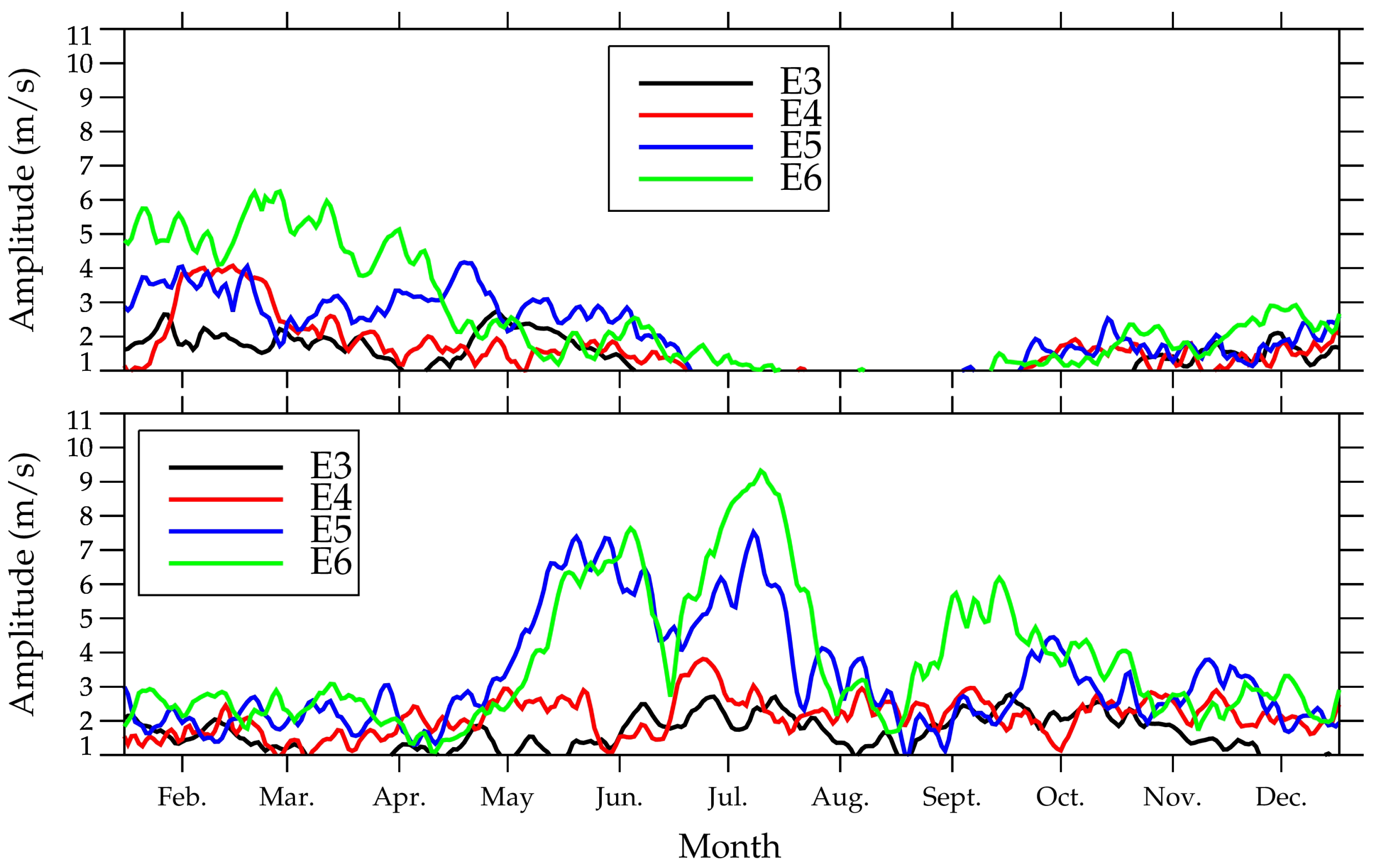
Figure 5 shows time–altitude contours of zonal wind amplitudes for E3, E4, E5 and E6 10DWs at 32° N in 2020. The time variations of these four waves show both similarities and differences. They are all strong in the spring and winter, and weak or even indiscernible in the summer and autumn, which is consistent with the seasonal variation of the subtropical jet (top row of Figure 1). This indicates that these wave activities and the eastward jets might be positively correlated. However, the strongest activities of these four waves occur in different months, and their magnitudes are also somewhat different. The largest amplitudes of the E3, E4, E5, and E6 10DWs are respectively about 5.6, 5.5, 6.2 and 5.4 ms⁻¹, which occur in November, February, March and January respectively.

Likewise, the time–altitude contours of zonal wind amplitudes for E3, E4, E5 and E6 10DWs at 32° S in 2020 are provided in Figure 6. Just like those in the NH, the time variations of these four waves display some similar and different characteristics. They are all not negligible throughout the year, and the amplitudes in spring, autumn and winter are greater than those in summer, which agrees well with the seasonal variation of the subtropical jet in the SH (bottom row of Figure 1). This also implies a positive correlation between the wave activities and the eastward jet. E5 is obviously the strongest mode, and E4 is stronger than E3 and E6. Similar to the situation in the NH, the strongest activities of these four waves in the SH occur in different months. The largest E3, E4, E5 and E6 10DW amplitudes in zonal wind are respectively about 4.9, 8.2, 10.5 and 5.6 ms⁻¹, which appear in September, June, May and July, respectively.

We highlight the evanescence regions where wave propagation is prohibited with red shadow in these two figures. The wave amplitude is large in the freely propagating region, while small in the evanescence region, obviously. In both hemispheres, there are very thick evanescence regions above the freely propagating regions at ∼15 km, which prevent these waves from propagating upward across the tropopause. As such, these eastward-propagating modes with large wavenumbers are weak or even disappear in the stratosphere and above. Since the background zonal wind within the whole display height range (0–32 km) at 32° N from July to August is westward or weakly eastward, there is an evanescence region.

The above result implies a positive correlation between the wave activities and the eastward jet. Then, the correlation coefficients between the amplitudes of E3, E4, E5 and E6 10DWs and the zonal-mean zonal wind at ∼11 km in 2020 is calculated. Figure 7 shows the zonal wind amplitudes of the eastward-propagating 10DWs with zonal wavenumbers from 3 to 6 at ∼11 km deduced from MERRA-2 data at 32° N and 32° S, respectively. A purple line marks the zonal-mean zonal wind. For a better representation, the zonal-mean zonal wind is scaled by a factor of seven. In both hemispheres, the seasonal variations of E3, E4, E5 and E6 10DWs are consistent with those of the zonal-mean zonal wind. The correlation coefficients between the E3/E4/E5/E6 10DWs and the zonal-mean zonal wind are shown in

Table 1. The correlation coefficients between the E3/E4/E5/E6 10DWs and the zonal-mean zonal wind.

Latitude	E3	E4	E5	E6
32° N	0.57	0.68	0.71	0.67
32° S	0.31	0.64	0.09	0.17

. All the coefficients except the one for the E5 10DW in the SH are far greater than the value corresponding to the 99% confidence level of a test of statistical significance, which imply strong and positive correlations. The coefficient for the E5 10DW also signifies a positive correlation but not as strong as the others. We speculate that there are other reasons for the time variation of the E5 10DW in addition to the background zonal wind.

It is well-known that PWs propagate predominantly westward (except equatorial Kelvin waves). This is due to their meridional fluctuation component and Coriolis force. Figure 8 shows the meridional wind amplitudes of the eastward-propagating 10DWs with zonal wavenumbers from 3 to 6 at ∼11 km deduced from MERRA-2 data at 32° N and 32° S, respectively. Kelvin waves are confined in low latitudes from 20° S to 20° N with no meridional components. The 10-day eastward-propagating modes presented in our paper are at 32° S and 32° N, and have significant meridional wind component. Therefore, they cannot be categorized as Kelvin waves.

6. Case Study of the Most Dominant Mode in the SH

Figure 7 shows that in the troposphere, the predominant 10DW mode in the SH, i.e., E5, is much stronger than the predominant 10DW mode in the NH. Its correlation with the background zonal wind indicates a complex time variation mechanism. Therefore, we further investigate the E5 10DW in the following section. The results in Figure 7 show that the E5 10DW was strongest on 12 May 2020, at ∼11 km in the SH. To confirm that this phenomenon was an enhanced event rather than a climatological variation, the daily amplitudes of the E5 10DW at 32° S and ∼11 km from 2006 to 2020 were obtained using the abovementioned fitting method.The arithmetic average of 15 amplitudes was taken as the climatological mean amplitude on each day. The climatological mean and standard deviations are shown in Figure 9. Under the assumption that the wave amplitudes basically follow the normal distribution [29], the mean value plus twice the standard deviation correspond to a 95% confidence level. Figure 9 shows that the amplitude on 12 May 2020, was larger than the climatological mean amplitude plus twice the standard deviation, which correspond to a 95% confidence level. Therefore, we postulate that the amplification of the E5 10DW on 12 May 2020, represents an enhanced event instead of a climatological variation.

Because the amplification of wave amplitudes is a dynamic process, we chose several dates at equal intervals to analyze the amplitude trend. Accordingly, the refractive index squared and the Eliassen–Palm (EP) flux and its divergence on 24 April, 30 April and 6 May were examined to explain the latitude–height structures and investigate the local excitation and dissipation processes. The EP flux and its divergence were analyzed by using the zonal transformed Eulerian mean momentum equation under the quasi-geostrophic approximation in spherical log (pressure) coordinates [41,42,43] by applying the formula below:

$${\overline{u}}_t+{\overline{v}}^{\ast }\left[{\left(acos\phi \right)}^{-1}{\left(\overline{u}cos\phi \right)}_{\phi }-f_0\right]+{\overline{w}}^{\ast }{\overline{u}}_z={\left({\rho }_{0}acos\phi \right)}^{-1}\nabla ·F$$

(5)

The vector F is known as the EP flux, of which the meridional and vertical components are defined, respectively, as follows:

$$F^{\left(\phi \right)}={\rho }_{0}acos\phi \left({\overline{u}}_z\frac{\overline{v^{\prime }{\theta }^{\prime }}}{{\overline{\theta }}_z}-\overline{u^{\prime }{v}^{\prime }}\right)$$

(6)

and

$$F^{\left(z\right)}={\rho }_{0}acos\phi \left\{\left[f_0-{\left(acos\phi \right)}^{-1}{\left(\overline{u}cos\phi \right)}_{\phi }\right]\frac{\overline{v^{\prime }{\theta }^{\prime }}}{{\overline{\theta }}_z}-\overline{u^{\prime }{w}^{\prime }}\right\}$$

(7)

where the prime symbol denotes a perturbation quantity (deviation from the zonal average); a, $\phi$ and ${\rho }_0$ are the same quantities as those in Equation (4); ${\overline{v}}^{\ast }$ and ${\overline{w}}^{\ast }$ are the meridional and vertical components, respectively, of the residual mean meridional circulation; u, v and w are the zonal, meridional and vertical winds, respectively; and $\theta$ is the potential temperature.

We obtain $\overline{u}$, $\overline{\theta }$ and ${\rho }_0$ from the MERRA-2 data, based on which $u^{\prime }$, $v^{\prime }$ and ${\theta }^{\prime }$ are obtained using the same fitting method mentioned above. Since the term proportional to $\frac{\overline{v^{\prime }{\theta }^{\prime }}}{{\overline{\theta }}_z}$ dominates the vertical EP flux component, the term proportional to $\overline{u^{\prime }{w}^{\prime }}$ is omitted from the calculations. In addition, the meridional and vertical components of the EP flux refer to a generalization of the group velocity concept so that their cross sections can be used to visualize the flow of the wave energy density [42,43,44]. Because of the density factors in Equations (5) and (6), the components of the EP flux have a large dynamic range. For a better height representation, the meridional and vertical components of the EP flux are scaled by the density, namely, $\frac{F^{\left(\phi \right)}}{{\rho }_0}$ and $\frac{F^{\left(z\right)}}{{\rho }_0}$ [19], which we refer to as EPY and EPZ, respectively, and display them as red vectors in the right panels in Figure 10. The zonal force per unit mass acting on the mean state is defined as $D_F={\left({\rho }_{0}acos\phi \right)}^{-1}\nabla ·F$, which is shown with color contours in the right panels in Figure 10. Regions of positive (negative) EP flux divergence are sources (sinks) of wave energy, where the wave is amplified (dissipated).

Figure 10 plots the refractive index squared, EP flux and its divergence on 24 April (top row), 30 April (middle row) and 6 May (bottom row). The red vectors of the EP flux in the right panels of Figure 10 indicate that the amplification of the E5 10DW at 32° S and ∼11 km was the result of the transmission of two wave energy flows. One flow started at 32–40° S and 3–4 km and propagated upward and then toward the equator, which we call an extratropical surface source. The other flow started from 39–49° S and 8–12 km and propagated almost horizontally toward the equator. On 24 April, the region at 49° S and 10 km was a source of the E5 10DW, as the EP flux divergence was indeed large and positive here with a maximum of 11.9 ms⁻¹ day⁻¹; the horizontal energy flow originated from this region. On 30 April, this source region moved to 47° S and 10 km, where the EP flux divergence also showed large positive values with a maximum of 7.1 ms⁻¹ day⁻¹. On 6 May, the source at 10 km shifted to 39° S with a maximum divergence of 7.9 ms⁻¹ day⁻¹. Otherwise, the zonal wind amplitudes of the E5 10DW in the left panel of Figure 10 show a bimodal structure in the latitude–altitude section. In addition to the abovementioned extratropic surface source, the sources at 49° S and 10 km on 24 April and at 47° S and 10 km on 30 April can explain the formation of the peak at 51° S and ∼11 km. In addition, the region where $n^2<0$ in the left panels and the red vectors of the EP flux in the right panels of Figure 10 both indicate that the energy flow of E5 10DW could not propagate upward from the tropospheric jet height to the stratosphere or across the equator into the NH.

The vertical components of the EP flux in Figure 10 show that the upward wave energy is dissipated at ∼15 km near the tropopause, which might lead to changes in the thermal structure of the tropopause. Then, the Lomb–Scargle periodogram analysis is performed on the time series of the cold point tropopause height (defined as the height of the minimum temperature) from 24 April to 11 May 2020, at Perth Airport. Due to the coarse vertical resolution of MERRA-2 data, only the result of radiosonde observations is shown in Figure 11. Clearly, the tropopause height has a significant spectral peak at the period range of 10DW. That is to say, the tropopause height is modulated by the wave energy deposition of E5 10DW, and exhibits short-term variability.

7. Conclusions and Discussion

Using radiosonde observations and MERRA-2 data, the characteristics of the mid-latitude 10DWs in the TLS of both the NH and the SH in 2020 were simultaneously studied. The main results and conclusions are as follows:

1. Single-site radiosonde observations in both hemispheres show that 10DWs exist in mid-latitudes in the TLS. In the troposphere of both hemispheres, strong 10DW activities are always accompanied by strong eastward jets (10–13 km) implying that the 10DW activities are related to eastward jets; this also implies that the 10DWs in the NH and SH might have a similar formation mechanism. In the lower stratosphere, 10DWs appear in boreal winter and spring as well as in austral winter and autumn. It should be noted that the 10DWs observed at a single site are the combination of multiple modes of the 10DWs with different zonal wavenumbers, the magnitude of which is greater than that of a single mode.

2. MERRA-2 data along latitude 32° N and 32° S show that the 10DW field in the troposphere is very different from the situation in the lower stratosphere. In the troposphere, 10-day waves exhibit prevailing eastward propagation over westward propagation, which agrees well with previous work [35]. Moreover, among these prevailing eastward-propagating modes, those with larger wavenumbers, i.e., E3, E4, E5 and E6 are stronger than those with smaller wavenumbers, i.e., E1 and E2, which is our new finding. In the troposphere, the eastward-propagating modes with larger wavenumbers dominate the 10DW field, while in the lower stratosphere, the 10DW field is dominated by modes with small zonal wavenumbers, i.e., W1, W2, E1 and E2, which is consistent with the previous studies [14,18,19]. The conclusions drawn from the MERRA-2 data in 2020 can also be obtained from the multi-year MERRA-2 data.

3. Further analyses on E3, E4, E5 and E6 modes in the troposphere of both hemispheres show that these four modes are positively correlated to the background zonal wind. The calculated refractive index squared reveals the control of background wind on these waves. For these four modes, weak eastward jets can cause negative refractive index squared. As such, these four modes’ activities are always accompanied by strong eastward jets. In addition, there are thick evanescence regions above ∼15 km, which prevent these waves from propagating upward across the tropopause. As such, these waves are not found in the stratosphere and above. In other words, the higher-order modes would encounter their critical layers not far from the source region due to their short vertical wavelengths and be dissipated there.

4. The temporal evolution characteristics of the 10DW modes reveal dramatic E5 10DW activity on 12 May 2020, at 32° S and ∼11 km. Then, a detailed case study of this E5 10DW activity indicates that was the most intense in the past 14 years and can be regarded as an enhanced event rather than a climatological variation. The refractive index squared and the EP flux and its divergence on three dates before the central date, i.e., 24 April, 30 April and 6 May, were further examined to explain the latitude–height structures and investigate the local excitation and dissipation processes. From this case study, we summarize three key conclusions. First, there are two sources of the E5 10DW: one source originates from the extratropical surface at mid-latitudes and shows first upward and then equatorward/poleward movement; the other source is located at 39–49° S and 8–12 km, and its energy flows horizontally to the equator/poles, leading to the formation of a bimodal structure in the latitude–altitude section. We note that the EP flux and its divergence reflect only the source and energy flow of waves, whereas the generation mechanism remains unclear. One source originates from the extratropical surface at mid-latitudes, which indicates the wave may be excited by irregular thermal or mechanical forcing there. Another source is near the zonal jet stream, which is always accompanied by strong baroclinic instability. We therefore speculate that baroclinic instability may be one candidate of the generation mechanisms. We further check the latitude–altitude sections of amplitudes of the E5 10DW on 12 May 2020 and find the maximum at (30° S, 11 km), where a powerful blocking anticyclone is present (referring to circulation maps https://earth.nullschool.net/ru/#2020/05/10/1800Z/wind/isobaric/250hPa/overlay=temp/orthographic=-350.63,-83.94,316/loc=14.739,-30.307 (accessed on 4 April 2022)). It seems that the blocking anticyclone might also be responsible for the E5 10DW intensification. However, the causal relationship among the three (blocking anticyclone, baroclinic instability and E5 10DW intensification) remains unknown and deserves further investigation. Second, the energy flow of E5 10DW cannot propagate upward across the tropopause and equatorward across the equator. Since there is a thick region of evanescence around the equator, the E5 10DW generated in one hemisphere does not affect the atmosphere in the other hemisphere. Third, the upward propagating wave energy of E5 10DW is deposited near the tropopause, leading to the modulations and short term variations of the thermal structure of the tropopause.