Abstract
This study aimed to determine the atmospheric conditions in which sea-effect snow (SES) and non-SES events occurred in a meso-scale structure. All snow events between 2009 and 2018 were found by examining the aviation reports at two international airports in Istanbul, Turkey. Then, threshold values and threshold intervals were presented for SES and non-SES events on the basis of many meteorological parameters (e.g., air temperature, dew point, relative humidity, heat fluxes, sea surface temperature (SST)). In addition, an algorithm was created for operational prediction of SES events at both airports. The most important parameter that distinguished SES events from NON-SES events was the temperature difference between sea surface (SS) and upper-atmosphere air parcel. Accordingly, sensible and latent heat fluxes had similarly higher values in SES events on average. Although the wind directions were mostly northerly in both event types, low wind shear in the layer between the SS and sub-inversion was prominent in SES events. For average snow depths, higher depths were measured in SES events than in non-SES events. In the same snow depth range, the heat fluxes were mostly high in SES events; on the other hand, the relative humidity values were lower.
Keywords:
sea-effect snowfall; air–sea interaction; Black Sea; Istanbul; snowfall forecast; aviation 1. Introduction
It is seen in many regions around the world that arctic, polar, and similar cold air masses incorporate heat and moisture fluxes depending on the temperature difference during their passage over any water body (e.g., lake, sea, and ocean) and leave this moisture loading in the form of snowfall on their route [1,2,3]. These snowfalls are expressed in the literature as lake-effect snow (LES) and sea-effect snow (SES) depending on the type of water source. Many studies of LES for the Great Lakes and Great Salt Lake (in the USA) are available in the literature. In the first studies, atmospheric conditions for LES formation were analysed [4,5], and the effects of meso- and synoptic-scale mechanisms were investigated [6,7]. Afterwards, operational forecasting methods were developed [7,8], climatological analyses were performed [9,10], and model projections were created [11,12,13]. Regarding the SES, analyses were performed for the Japan Sea [14,15], Caspian Sea [16,17,18], Adriatic Sea [19], Baltic Sea [20], and Black Sea [21,22,23,24]. In these studies, similarly to those in the Great Lakes, the atmospheric conditions, climatology, and predictions of SES were investigated. The SES event that occurred in eastern Massachusetts (in the USA) in 1999 was one of the rare events with the effect of ocean forcing [25].
In studies on the determination and prediction of precipitation types (rain, snow), the most important meteorological parameter was the critical air temperature value [26,27,28]. In addition, discrimination can be made based on particle characteristics using remote sensing products (satellite and radar images) [29]. In order to make a similar distinction between snowfall and LES/SES, threshold values of various meteorological parameters were set, and operational classifications were made according to the morphological characteristics of snow bands using remote sensing products. The threshold values for some key parameters in LES and SES in the literature are as follows:
- Fetch distance: The distance that the cold air parcel travels over the relatively warmer water body should be long enough [4,7,30,31,32,33]. This distance determines how much heat and moisture flux will be taken from the lake/sea surface (LS/SS) [34,35]. The amount of snowfall increases depending on the increase in this distance [5,36]. For enhanced lake/sea effect snow, the fetch distance should be at least 80 km. If there is no synoptic scale support, this distance should be a minimum of 160 km for pure LES [8].
- Inversion layer: The existence of a mechanism that limits the convection that starts on the water body at higher levels often contributes to the development of LES/SES and increases their intensity [5,37,38]. It also affects their morphological structure and trajectory [7]. The formation of this layer in the range of 1000–850 hPa has a negative effect, as it will limit the convection early. Accordingly, band formations cannot be observed, or weak bands occur [39,40,41]. When the inversion layer is deeper and located at higher atmospheric levels, the unstable layer deepens, allowing the LES/SES to increase in intensity [7,42].
- Temperature difference: The high temperature difference between the upper level air parcel and the LS/SS is one of the most important parameters for LES/SES band formation [43,44,45,46,47]. It was revealed that the difference between 850 hPa and LS/SS should be a minimum of 13 °C [2,7,37,38,40,48], while the difference between 700 hPa and LS/SS should be a minimum of 16–17 °C [7,41,49]. It was also stated that vertical fluxes of momentum, heat and moisture decrease depending on the decrease in temperature differences [31].
- Wind speed and direction: Variations in wind speed and direction between LS/SS and upper levels play an important role in the formation, development and dissipation of LES/SES bands [7,49,50,51,52]. The difference in wind speed has two different consequences. If the wind speed is high, more heat and moisture flux are transferred from the LS/SS to the air parcel. However, there is not enough time for this transfer at short fetch distances. Therefore, high wind speeds at long fetch distances and lower wind speeds at short fetch distances contribute positively to band formation [53]. Suriano and Leathers found the average wind speed for the Great Lakes to be between 8–17.3 kt [54]; Campbell and Steenburgh found this value to be 5.8–11.7 kt for Tug Hill in New York State, USA [55]. Directional wind shear of 60° and below between 700 hPa and LS/SS supports band formation, while higher changes cause bands to disperse [7,32,41]. Stronger band formations are observed at 30° wind shear and below [7,54,56].
- Heat Fluxes: One of the most important factors in the formation of LES/SES is how much heat and moisture flux will be transferred from the warm water surfaces to the air parcel above. Due to the air–sea interaction, heat and moisture fluxes moving from the water surfaces destabilize the lower atmospheric layer [57], and a shallow convection layer forms [38,58,59]. This layer generally varies according to the downstream wind direction and strength, the shape of the water body, and the presence of synoptic-scale systems [38]. Lang and co-workers stated that the sensible and latent heat flux values for Lake Erie and Lake Ontario were 50–150 W m−2 at times with LES [53], while Sousounis and Mann determined that wind speeds in the range of 10–15 kt on the lake produce sensible and latent heat flux in the range of 200–500 W m−2 [60].
- Humidity: In LES/SES studies, specific and relative humidity parameters were analysed. Wiley and Mercer (2000) found that the specific humidity value is in the range of 2.5–3.0 g kg−1 in heavy snowfalls in the Great Lakes [47]. Relative humidity values were determined as 80–90% at 850/700 hPa levels for the heavy snowfalls due to SES [22,23].
Throughout the history of Istanbul, snowfalls have sometimes become a meteorological disaster. In the first half of the 20th century, the Bosphorus, the Golden Horn, and the dams were frozen, which prevented electricity and water needs from being met [61]. In 1987, snowfalls that continued for days under the effect of cyclone and atmospheric blocking caused snow depths in the order of meters. Electricity and water cuts were experienced, and disruptions and cancellations occurred in all types of transportation [62]. In the 2000s, heavy snowfall occurred four times, and snow depths between half a meter and one meter were measured in areas affected by cyclone and SES bands. Especially in the 21st century, snowfalls have negatively affected aviation activities at airports in Istanbul. These effects can often lead to flight cancellations and various accidents or incidents. In a study examining the accident-incident reports in the European region between 2005 and 2014, the effect of weather conditions was found to be 15% among the accident-causing factors. Most of the adverse weather conditions were the occurrence of events that reduce horizontal visibility (heavy snowfall and rainfall, fog) and cause icing [63]. In this study, an analysis of snow events that took place in Istanbul was performed. Between 2009–2018, SES and non-SES events were differentiated using satellite images for the snow events determined from the two airport reports. Then, the threshold values were determined due to the changes in meteorological parameters (surface air temperature, surface dew point, relative humidity, pressure, wind speed/direction), the results of air–sea interaction (sea surface temperature—SST, specific humidity, latent and sensible heat fluxes, inversion layer), and the changes in the amount of snowfall (snow depth). The goal of the study was to develop an algorithm that will allow nowcasting and forecasting of SES events at both airports. Accordingly, information in the literature on SES events and the meteorological parameters affecting them is presented in Section 1; the study area, airports, and the data used were introduced, and the method is specified in Section 2. Statistical analyses of SES and non-SES events were performed at both airports during the period, snow depth analyses were conducted for both event types, and a 12-item algorithm was developed to identify SES events, as presented in Section 3. Finally, general evaluations of the results of the study are given in Section 4.
2. Materials and Methods
The meso-scale analysis of snow events that occurred in Istanbul province between 2009–2018 was carried out. Istanbul is located in the Marmara Region, which is the most economically and industrially developed region of Turkey. While Black Sea climate features are observed in the northern parts of Istanbul with hot summers, mild winters and precipitation in all seasons and Mediterranean climate characteristics are observed in the southern parts with hot, dry summers and warm, rainy winters. A large part of the population in the province is located in the southern part of the region. In the city, which does not have significant elevation, precipitation variability is observed in the north–south direction. Istanbul is the only city that has a coastline on the Black Sea and the Marmara Sea, has the Bosphorus between these two seas, and has land on both the Asian and European continents. Istanbul Atatürk International Airport (ICAO Code: LTBA) and Istanbul Sabiha Gökçen Airport (ICAO Code: LTFJ) are located on two different continents. Their height above sea level is in the range of 50–100 m [64]. The Istanbul Kartal Radiosonde station, where meteorological parameters of the upper atmospheric levels were provided, is located on the Asian continent and is at approximately sea level. The information about the study area, the airports and radiosonde station where the data were provided, and the specific points determined on the western Black Sea are shown in Figure 1.
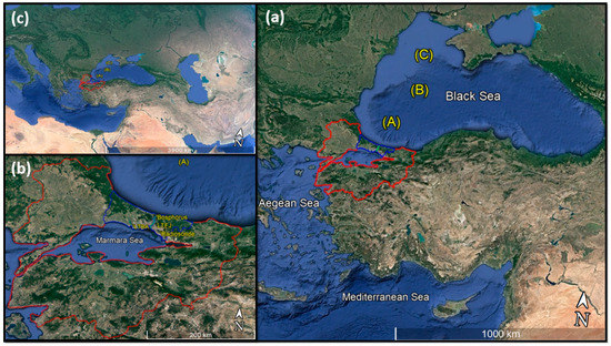
Figure 1.
Study area. The large black rectangle shows the study area (a), the black square in the lower left shows the study area in detail (b), and the black square in the top left shows the study area in large scale (c). The area covered with red lines shows the Marmara Region. The area covered with blue lines within the red lines shows Istanbul. The green line, which cuts the blue lined area almost in half, represents the Bosphorus. The west of this line is the European Continent, and the east is the Asian Continent. The locations of LTBA, LTFJ, and Istanbul Kartal Radiosonde Station are indicated in the figure. The coordinate information of points A, B, and C are as follows, respectively: 29.5° E, 42.5° N; 30.5° E, 43.5° N; 30.5° E, 44.5° N.
The Meteorological Aerodrome Reports (METARs) and the Meteorological Aerodrome Special Reports (SPECIs) published by the LTBA and LTFJ were obtained from the IOWA Environmental Mesonet website accessible by Iowa State University [65]. Since both airports are international airports, METAR reports contain real data published at half-hourly intervals. SPECI reports are published when situations affecting aviation activity arise between two METAR reports. The air temperature (T), dew point (Td), relative humidity (RH), pressure (P), snow depth, wind speed (Ws), and wind direction (Wd) data from surface level meteorological parameters were provided from these reports for the years 2009–2018. The information on the upper atmospheric level meteorological parameters (T, Td, Ws and Wd at 850, 700 and 500 hPa levels; inversion layers between surface–850 hPa, 850–700 hPa, and 700–500 hPa) was obtained from the sounding data provided by the Istanbul Kartal Radiosonde station. These data are the actual observation data obtained from the measurement devices connected to a meteorological balloon that is sent into the atmosphere twice a day (at 0000 and 1200 UTC). These data were accessed from the University of Wyoming Atmospheric Science’s website [66].
After the determination of snow events in Istanbul, various satellite images were used to distinguish between the SES and non-SES events. At this stage, the study in which SES bands were classified according to the morphological structure within the same period for the same study area was taken as reference [22]. Satellite images of all times with snowfall were re-examined and confirmed by the method of detecting LES bands by means of satellite images for the eastern United States [38]. First, the Moderate Resolution Imaging Spectroradiometer (MODIS) module images of the Terra satellite were examined. Although this module offers high resolution (0.25° × 0.25° latitude–longitude resolution) images, it only provided one image per day for the study area. The images from the module were obtained from the National Aeronautics and Space Administration (NASA) [67]. Then, some of the second-generation MSG-2 and MSG-3 satellite products of the Meteosat satellite series were analysed. MSG-2 and MSG-3 provide images at 15 min intervals, covering the continents of Europe and Africa. In this study, satellite images on different channels of the spinning enhanced visible and infrared imager (SEVIRI) radiometer on the MSG-2 and MSG-3 satellites were evaluated. Infrared (channel 9), visible band (channel 321) and airmass satellite images were analysed in detail throughout the entire period at 15 min intervals. These data have a resolution of 3 km [68]. The SEVIRI radiometer images used in the study were obtained from the Turkish State Meteorological Service (TSMS) [69].
The SST information was obtained from NOAA High-Resolution Blended Analysis in order to analyse air–sea interactions. The data with a latitude–longitude resolution of 0.25° × 0.25° were analysed for three different points (“A”: 29.5° E, 42.5° N; “B”: 30.5° E, 43.5° N; “C”: 30.5° E, 44.5° N) determined in the western Black Sea within the entire snowy period. The data consist of a global scale grid of multiple observation data obtained from satellites, buoys, and floats. The data, which present average daily SST values, were obtained from the Asia-Pacific Data-Research Center (APDRC) [70]. In addition, in order to detect the heat fluxes from the SS to the upper atmosphere, sensible and latent heat flux data at the level of 1000 hPa were obtained for the three points (A, B, C) determined in the study from the Woods Hole Oceanographic Institution (WHOI)—Objectively Analyzed Air-Sea Fluxes (OAFlux) data set. Specific humidity data for the 1000 hPa level were also taken from the same data set. The data set is a product created by integrating satellite observations, ship reports, and atmospheric model data run with reanalysis data. All of these data are presented as daily average values [71].
In the study, statistical significance levels of the average values were examined for all discrete data sets analysed for SES and non-SES events (except for wind direction information and inversion conditions). Data belonging to the same meteorological parameter from both even types were first subjected to a normality test (Kolmogorov–Smirnov test). Since no significant deviation from the normal distribution was observed in all of the data sets, the t-test was applied. p-values and interpretations obtained by applying the independent two samples t-test are given in Table 1.

Table 1.
The degrees of statistical significance of the data sets analysed in the study for SES and non-SES events.
At the end of the study, a 12-item algorithm was developed for LTBA and LTFJ to be used in the operational estimation of SES events. The algorithm was then validated with reference to a total of three different SES events that occurred separately and simultaneously at both airports. In these events, the algorithm scored 11 out of 12 (92%) and 12 out of 12 (100%).
3. Results
3.1. SES and Non-SES Events
A total of 118 days of snowfall were identified at LTBA and LTFJ between 2009 and 2018. According to the analyses made with satellite images, 73 days were detected as SES events and 45 days as non-SES events. At LTBA, 57 days of SES events and 28 days of non-SES events were determined, while similarly at LTFJ, 72 days of SES events and 38 days of non-SES events were recorded. Total snowfall duration at LTBA was found to be 632 h for SES events and 215 h for non-SES events. At LTFJ, these values were 745 h and 260 h, respectively. No SES events were observed in 2009; the most SES and non-SES events occurred in 2012 (Figure 2a). On a monthly basis, it was observed that both SES and non-SES events occurred mostly in January and least often in March (Figure 2b).
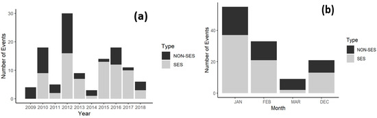
Figure 2.
Annual distribution of sea-effect snow (SES) and non-SES events in the left panel (a), monthly distribution in the right panel (b).
3.2. Meteorological Conditions at LTBA and LTFJ
At both airports, the average air temperature, dew point and relative humidity were higher in non-SES events (Figure 3). On the other hand, average wind speed values were close to each other. In the presence of SES events at LTBA, the average air temperature was −0.1 °C, dew point −2.4 °C, wind speed 14.4 kt, and relative humidity 84.3%, while in the presence of non-SES events, the average values were 0.5 °C, −0.5 °C, 16 kt and 89.6%, respectively (Figure 3a). In the presence of SES events at LTFJ, the average air temperature was 0 °C, dew point −2.2 °C, wind speed 10.6 kt, and relative humidity 86.1%, while in the presence of non-SES events, the average values were 0.5 °C, −0.8 °C, 9.3 kt and 91.5%, respectively (Figure 3b). Temperature and dew point values showed a wider variation in SES events than in non-SES events at both airports. Although almost similar variations were observed in wind intensities, relative humidity values also showed much larger variation in SES events than in non-SES events (Figure 3).
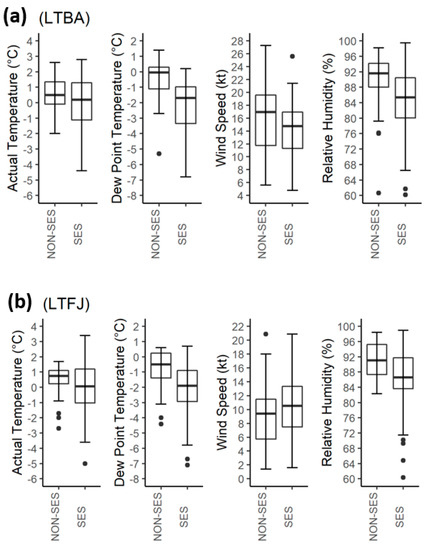
Figure 3.
The comparison of meteorological parameters in SES and non-SES events at (a) LTBA and (b) LTFJ.
In the SES and non-SES events, the prevailing wind direction information observed at the airports is given in Table 2. While it was observed that the northerly winds predominate (NW, N, NE) at both airports in SES events, almost similar results were observed in non-SES events. The most significant difference between SES and non-SES in terms of prevailing wind direction was that variable wind conditions (VRB) were observed more in non-SES events. In addition, a small amount of westerly and south-westerly wind directions were also observed in non-SES events. In the studies carried out for the Caspian Sea, which is located at almost the same latitudes as the Black Sea, it was determined that the prevailing wind direction in SES events is mostly northerly [17,18].
Table 2.
The wind direction frequencies in SES and non-SES events at LTBA and LTFJ.
3.3. Meteorological Conditions on the Western Black Sea
In the formation of SES bands that caused SESs at LTBA and LTFJ, the water source where the necessary heat and moisture fluxes were supplied was the western Black Sea. In this direction, within the scope of the study, three different points were selected to observe the changes in the specific humidity, heat fluxes and, SST over the western Black Sea in SES and non-SES events. These points are shown in Figure 1. The changes in the aforementioned parameters at each point are given in Figure 4a–c. The data obtained at three different points for four different parameters were handled separately to observe the effects on the formation, development and dissipation processes of SES bands. The main reason for choosing these points is that the coordinates for each data set exactly coincide with the grid points.
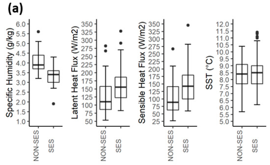
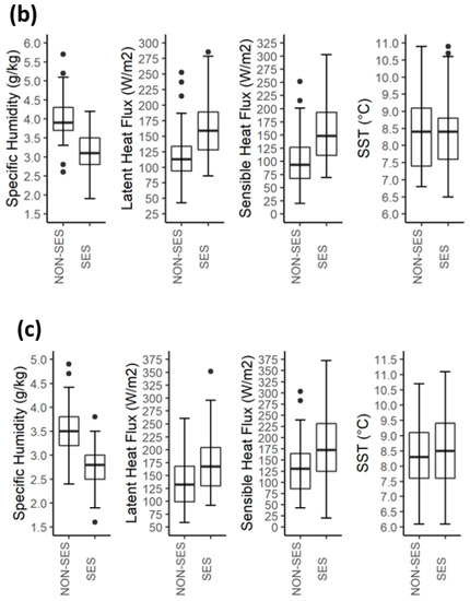
Figure 4.
Changes in meteorological parameters in SES and non-SES events at (a) point “A”, (b) point “B”, and (c) point “C” on the western Black Sea surface.
Specific humidity values were observed to be between 17.5% and 22.5% lower in SES events than in non-SES events at all three points. The highest mean values were observed at point “A” and the lowest values at point “C”. The average latent heat flux values were 27% higher at point “A”, 37% higher at point “B”, and 25% higher at point “C” in SES events compared to non-SES events. The average sensible heat flux values were found to be 27% higher at point “A”, 37% at point “B”, and 25% higher at point “C” in SES events compared to non-SES events. In both heat fluxes, the highest values in SES events were observed at point “C” and the lowest values at point “A”. In SST values, the average value in SES events was determined as 8.5 °C at all three points. Relatively lower average values (2–3% less) were found in non-SES events. The results obtained in this section, especially regarding heat fluxes, are similar to those of many studies in the literature [38,56,58,59]. Lang and co-workers stated that in cases of sufficient fetch distance, the wind speed varies in direct proportion to the heat and moisture fluxes upwards from the SS [53]. Additionally, Sousounis and Mann stated that 10–15 kt high wind speeds generate heat fluxes in the range of approximately 200–500 W m−2 [60]. In this study, high wind speed values were observed over the sea when high sensible and latent heat flux values were observed (not shown). Increasing wind speed values make a positive contribution to heat and moisture fluxes, as there is sufficient fetch distance (400–600 km) over the western Black Sea; on the other hand, they make a negative contribution to the specific humidity values on the SS. For this reason, lower specific humidity values were observed in SES events compared to non-SES events.
3.4. Air–Sea Interaction over the Western Black Sea
One of the most important parameters that plays a role in the occurrence of LES/SES events is a certain temperature difference between the cold air mass and the relatively warmer water source over which it passes. In this regard, some limit values have been revealed in the studies conducted for different regions where LES/SES events were observed (Section 1). In this study, the average ΔTSS-850 value was found to be 17.6 °C for SES events and 12.2 °C for non-SES events (Figure 5a). Similarly, the average ΔTSS-700 value was found to be 24.9 °C for SES events and 19.3 °C for non-SES events (Figure 5a). In SES events, the highest ΔTSS-850 value was 24.1 °C and the highest ΔTSS-700 value was 33.1 °C. The lowest temperature differences for ΔTSS-850 and ΔTSS-700 were 9.8 °C and 14.6 °C, respectively. In addition, 94% of the ΔTSS-850 data was 13 °C and above, and 99% of the ΔTSS-700 data was 17 °C and over. In these analyses, point “B” was taken as a reference for SST information (Figure 5a,b). Similar results were obtained in the analyses made on the other two points determined on the western Black Sea.
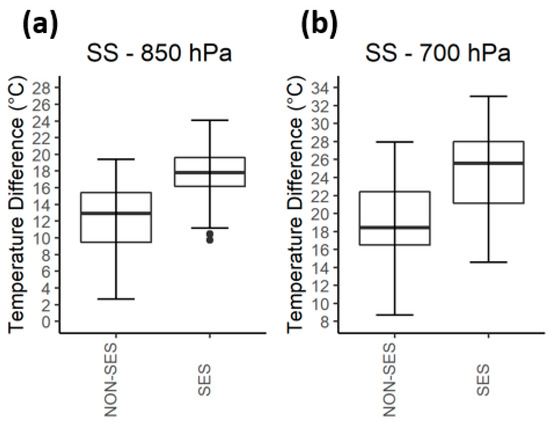
Figure 5.
The variation in the temperature difference between the upper atmospheric level air (850 and 700 hPa levels) and point “B” (specified on the western Black Sea surface) in SES and non-SES events. (a) the temperature difference between the 850 hPa level and point “B”, (b) the temperature difference between the 700 hPa level and point “B”.
Wind speed and direction changes in the convective layer (especially just below the inversion layer) have an important effect on the formation, intensity and trajectory of the LES/SES bands. The low wind direction change from the LS/SS to the upper atmospheric levels is an important parameter that increases the formation and strength of the bands. Regarding this, in the literature, between LS/SS and 700 hPa, 30° and below were specified as the appropriate range for strong band formations, and 60° and below for band formation [7,32]. In this study, wind direction changes between 850/700 hPa levels and point “B” specified on the western Black Sea (ΔWSS-850 and ΔWSS-700) are discussed separately for SES and non-SES events. In SES events, the ΔWSS-700 value was 60° and below at a rate of 59%, while this rate decreased to 26% in non-SES events. The ΔWSS-850 value was 60° and below in both SES and non-SES events, at rates of 71% and 52%, respectively (Table 3).
Table 3.
Wind shear between the western Black Sea surface (point “B”) and upper atmospheric levels (850 and 700 hPa) in SES and non-SES events.
The variation in the wind speed over the LS/SS up to the upper atmospheric levels is a critical parameter that determines the band structures and formations as well as the wind direction changes [54]. In this study, wind speed differences between 850/700 hPa levels and SS were observed in a relatively narrow range in SES events compared to non-SES events. This difference was 12.1 kt for ΔWSSS-850 (Figure 6a) and 14.1 kt for ΔWSSS-700 (Figure 6b) in SES events, while it was 14.5 kt (Figure 6a) and 18.4 kt (Figure 6b) in non-SES events, respectively.
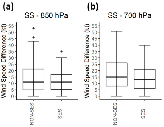
Figure 6.
The variation in the wind speed difference between the upper atmospheric levels (850 and 700 hPa levels) and point “B” (specified on the western Black Sea surface) in SES and non-SES events. (a) the wind speed difference between the 850 hPa level and point “B”, (b) the wind speed difference between the 700 hPa level and point “B”.
The limitation of the convective boundary layer, which develops due to the air–sea interaction, at the upper atmospheric levels is important in the LES/SES band formation. The formation of this layer in the first 150 hPa from LS/SS is stated to be unfavourable in terms of band formation [41], while its presence at higher atmospheric levels increases baroclinity and contributes to strong band formations [38,40]. In this study, an inversion layer between SS and 500 hPa was observed in 79.5% of SES events, while this rate was 67.9% in non-SES events. Additionally, in SES events, the proportion of inversion layers occurring only within the first 150 hPa was 4.8%, whereas in non-SES events, this rate was 25%. The presence of an inversion only between 850–500 hPa, which is important for the formation of strong SES bands, was 61% in total in SES events and 33.3% in non-SES events (Table 4).
Table 4.
Presence and location of inversion layers in SES and non-SES events.
3.5. Snow Depths and Influencing Meteorological Parameters in SES and Non-SES Events
In the SES events, the maximum daily fresh snow depths measured at LTBA and LTFJ were 35 cm and 36 cm, respectively. In non-SES events, these values were measured as 7 cm and 13 cm, respectively. The dates on which the maximum fresh snow depths were measured were different at both airports. At LTBA, most of the daily fresh snow depths in SES events occurred at 1 cm and below, and a significant amount was between 1–5 cm. In addition, values over 15 cm were measured at a rate of 8%. On the other hand, in non-SES events, a larger part of the daily fresh snow depths occurred at 1 cm and below compared to SES events, while the ratio of values measured between 1–5 cm was similar. In addition, values above 10 cm did not occur. At LTFJ, daily fresh snow depths in SES events were similar to those at LTBA. The most important differences were that the ratios of 1–5 cm and over 15 cm were higher at LTFJ. Unlike non-SES events at LTBA, measurements were made in the range of 11–15 cm in non-SES events at LTFJ, and measurements of 1 cm and above were also found at a higher rate (Figure 7).
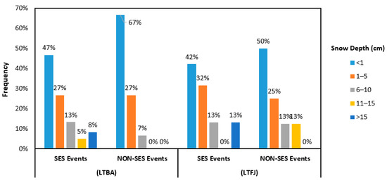
Figure 7.
Distribution of snow depths in SES and non-SES events at LTBA and LTFJ.
In SES and non-SES events, changes in snow depths depending on meteorological parameters were analysed for both airports (Table 5 and Table 6). For each snow depth range in Figure 7, SES and non-SES events were handled separately. In this process, the average meteorological parameter values at the airport, SS and upper atmospheric levels were determined. At both airports, snow depths often increased in both SES and non-SES events as air temperatures decreased. The average dew point depression (T-Td) was mostly higher in SES events than in non-SES events. Moreover, as dew point depression decreased in both SES and non-SES events, snow depth mostly increased for both airports. The average wind speed values were higher in non-SES events compared to SES events, and as the snow depth increased, wind intensity was generally higher in both events. In all SES events, northerly wind directions were dominant; on the other hand, in non-SES events, although similarly northerly directions were dominant, variable wind directions were also semi-dominant. The average relative humidity values were directly proportional to snow depths at both airports during SES events. This trend was mostly observed in non-SES events. At snow depths above 1 cm, the minimum relative humidity value was 84.3% at LTBA and 86.2% at LTFJ for both types of events. The average pressure values were mostly measured higher at LTBA than at LTFJ in both events. The average pressure values in SES events were found in the range of 1022–1024 hPa at LTBA and in the range of 1016.5–1019.4 hPa at LTFJ (excluding snow depths over 15 cm). The average ΔTSS-850 values were found to be a minimum of 16.7 °C (at LTFJ) and a maximum of 19.7 °C (at LTFJ) in SES events. In non-SES events, these values were 4.7 °C (at LTFJ) and 15.8 °C (at LTFJ), respectively. The average ΔTSS-700 values were found to be a minimum of 22.8 °C (at LTFJ) and a maximum of 27.9 °C (at LTFJ) in SES events. In non-SES events, these values were 15.0 °C (at LTFJ) and 21.1 °C (at LTFJ), respectively. The average sensible and latent heat flux values were higher for SES events than for non-SES events at both airports at the same snow depth ranges. In SES events, the highest flux values were observed at snow depths above 15 cm. The average specific humidity values, on the other hand, were higher in non-SES events than in SES events, which were the exact opposite of flux values at the same snow depths. Minimum values in SES events were also observed at the highest snow depth. Almost all SES events had one or more inversion layers. In non-SES events, this rate was half as low as in SES events.
Table 5.
Average values of meteorological parameters in SES and non-SES events according to snow depth intervals at LTBA.
Table 6.
Average values of meteorological parameters in SES and non-SES events according to snow depth intervals at LTFJ.
3.6. An Algorithm for the Prediction of SES Events at LTBA and LTFJ
In this study, SES and non-SES events were analysed at the meso-scale. In this context, the changes in many meteorological parameters in both types of events, both at airports and on/over the sea, were analysed separately, and the results were shared. After revealing the difference between SES and non-SES events at meso-scale, the changes in average meteorological parameter values from small to large were identified in the frequency ranges determined for the times when SES events occurred at LTBA and LTFJ (Figure 8).
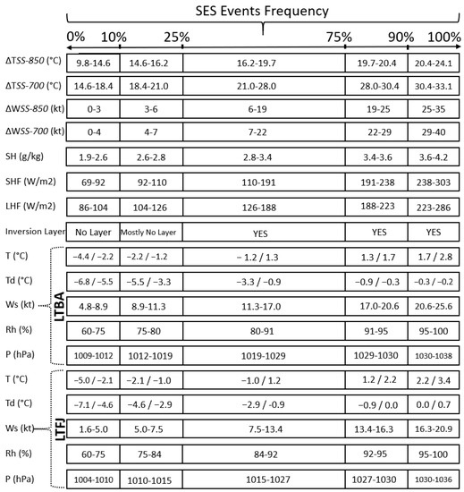
Figure 8.
Changes in average meteorological parameter values in SES events at LTBA and LTFJ.
A 12-item algorithm was created for the operational prediction of SES events at LTBA and LTFJ. Each of these conditions is important for the formation, development and trajectory of SES bands over the western Black Sea. All of the conditions specified in the algorithm below were met in 90% of the SES events that occurred at LTBA and LTFJ. As stated in Table 1, since the air temperature and wind speed values at the airports in SES and non-SES events were not statistically significantly different from each other, at least 10 conditions out of the 12 should be expected to be met (usually condition 9 and/or condition 12 were/was not met in 10% of the SES events). It was observed that in some rare cases where more than two conditions were not met (at most, four conditions were not met), one or more of the additional conditions listed at the bottom of the algorithm occurred. Additionally, these additional conditions increased the severity of the SES events (i.e., strengthening of the bands, increasing the amount of snowfall, etc.). Besides all of the conditions of this 12-item algorithm and additional conditions, the formation of suitable atmospheric conditions at airports and the monitoring the formations and trajectories of SES bands with remote sensing products (e.g., radar and satellite observations) have critical importance in terms of determining the regions to be affected by SES bands. The Algorithm 1 created for the SES prediction is as follows:
| Algorithm 1. For the SES prediction at LTBA and LTBJ (in Istanbul) |
|
4. Discussion and Conclusions
One of the most important parameters that negatively affects operational activities in the aviation sector is adverse weather conditions [72,73]. Meteorological events that reduce or obstruct visibility can cause accident-incident events, especially during the landing and take-off phases [63,74]. Snowfall and SES are meteorological parameters that reduce visibility. SES bands can cause long-term heavy snowfalls in narrow or wide areas depending on their formation and inland extension. The type and trajectory of these bands can usually be detected on radar images. However, knowing the answers to the following questions in nowcasting/forecasting applications will contribute to operational forecasts. (1) What are the atmospheric conditions required for SES bands to begin to form over water bodies (at SS and upper atmospheric levels) and, accordingly, when will they begin to form/dissipate? (2) How will they behave with the effect of atmospheric conditions at surface and upper atmospheric levels on their trajectory along their inland extension, and what will be the surface level types of precipitation? In this study, the analyses of meteorological parameters at surface level, SS and upper atmospheric levels affecting SES were performed, value ranges were determined for two international airports, and a 12-item algorithm was created to contribute to operational activities.
Although the atmospheric conditions for the formation of SES and SES bands in similar studies in the literature were often similar in this study, some different results also emerged. For example, 13 °C and 17 °C threshold values for ΔTSS-850 and ΔTSS-850 have been determined in the literature, respectively [7,37,40,48,49]. In this study, these values were 17.6 °C and 24.9 °C on average, respectively. The most important reason for this is that SES events are mostly supported by synoptic-scale systems. SES events that occur in this way are called sea-enhanced snow. Similarly, for the formation of SES bands, certain threshold values are available for wind speeds and vertical wind variation. In this study, SES band formations were also observed above these threshold values. The main reason for this is that the fetch was at least two times longer than the fetches in the studies in the literature. This situation does not prevent the high wind speeds at sub-inversion level from adding the necessary heat and moisture fluxes to the air parcel since the distance covered over the sea is long. The sensitivity of strong SES bands, which occur in parallel with high heat and moisture fluxes, to wind direction changes also decreased in this way.
Finally, the 12-item algorithm for LTBA and LTFJ was validated by selecting various cases. In this context, three of the events were selected. One of them was chosen from events that took place at LTBA only, one at LTFJ only, and finally one at both airports. Then, the data on these events were extracted from all the data sets analysed in the algorithm. Later, the revised algorithm was analysed separately for these three events. The results were as follows: 11 out of 12 items in the algorithm were met for the event that occurred at LTBA, 11 out of 12 for the event that occurred at LTFJ, and 12 out of 12 for the event that occurred at both airports.
Author Contributions
Conceptualization, V.Y., A.R.L., N.I.F. and A.D.; methodology, V.Y.; writing—original draft preparation, V.Y.; writing—review and editing, V.Y., A.R.L., N.I.F. and A.D. All authors have read and agreed to the published version of the manuscript.
Funding
This work was supported by the Turkish Science Foundation (TUBITAK) with Grant Number 1059B142000051.
Institutional Review Board Statement
Not applicable.
Informed Consent Statement
Not applicable.
Data Availability Statement
Not applicable.
Acknowledgments
This work was supported by the Turkish Science Foundation (TUBITAK) with Grant Number 1059B142000051. The authors would like to thank the Turkish State Meteorological Service for the data used in this study.
Conflicts of Interest
The authors declare no conflict of interest.
References
- Kristovich, D.A.R.; Young, G.S.; Verlinde, J.; Sousounis, P.J.; Mourad, P.; Lenschow, D.; Rauber, R.M.; Ramamurthy, M.K.; Jewett, B.F.; Beard, K.; et al. The Lake—Induced Convection Experiment and the Snowband Dynamics Project. Bull. Am. Meteorol. Soc. 2000, 81, 519–542. [Google Scholar] [CrossRef]
- Kunkel, K.E.; Wescott, N.E.; Kristovich, D.A.R. Assessment of potential effects of climate change on heavy lake-effect snow-storms near Lake Erie. J. Great Lakes Res. 2002, 28, 521–536. [Google Scholar] [CrossRef]
- Cordeira, J.M.; Laird, N.F. The Influence of Ice Cover on Two Lake-Effect Snow Events over Lake Erie. Mon. Weather Rev. 2008, 136, 2747–2763. [Google Scholar] [CrossRef]
- Wiggin, B.L. Great Snows of the Great Lakes. Weatherwise 1950, 3, 123–126. [Google Scholar] [CrossRef]
- Petterssen, S. Weather Analysis and Forecasting; McGraw Hill: New York, NY, USA, 1956; Volume II, p. 266. [Google Scholar]
- Peace, R.L.; Sykes, R.B., Jr. Mesoscale study of a lake effect snowstorm. Mon. Weather Rev. 1966, 94, 495–507. [Google Scholar] [CrossRef]
- Niziol, T.A. Operational Forecasting of Lake Effect Snowfall in Western and Central New York. Weather Forecast. 1987, 2, 310–321. [Google Scholar] [CrossRef]
- Dockus, D.A. Lake effect snow forecasting in the computer age. Natl. Weather Dig. 1985, 10, 5–19. [Google Scholar]
- Alcott, T.I.; Steenburgh, W.J.; Laird, N.F. Great Salt Lake-effect precipitation: Observed frequency, characteristics, and asso-ciated environmental factors. Weather Forecast. 2012, 27, 954–971. [Google Scholar] [CrossRef]
- Laird, N.; Bentley, A.M.; Ganetis, S.A.; Stieneke, A.; Tushaus, S.A. Climatology of Lake-Effect Precipitation Events over Lake Tahoe and Pyramid Lake. J. Appl. Meteorol. Clim. 2016, 55, 297–312. [Google Scholar] [CrossRef]
- Theeuwes, N.E.; Steeneveld, G.J.; Krikken, F.; Holtslag, A.A.M. Mesoscale modeling of lake effect snow over Lake Erie—Sensitivity to convection, microphysics and the water temperature. Adv. Sci. Res. 2010, 4, 15–22. [Google Scholar] [CrossRef][Green Version]
- Notaro, M.; Bennington, V.; Vavrus, S. Dynamically Downscaled Projections of Lake-Effect Snow in the Great Lakes Basin. J. Clim. 2015, 28, 1661–1684. [Google Scholar] [CrossRef]
- Saslo, S.; Greybush, S.J. Prediction of lake-effect snow using convection-allowing ensemble forecasts and regional data assim-ilation. Weather Forecast. 2017, 32, 1727–1744. [Google Scholar] [CrossRef]
- Estoque, M.A.; Ninomiya, K. Numerical simulation of Japan Sea effect snowfall. Tellus 1976, 28, 243–253. [Google Scholar] [CrossRef]
- Veals, P.G.; Steenburgh, W.J.; Nakai, S.; Yamaguchi, S. Factors Affecting the Inland and Orographic Enhancement of Sea-Effect Snowfall in the Hokuriku Region of Japan. Mon. Weather Rev. 2019, 147, 3121–3143. [Google Scholar] [CrossRef]
- Nicholls, J.F.; Toumi, R. On the lake effects of the Caspian Sea. Q. J. R. Meteorol. Soc. 2014, 140, 1399–1408. [Google Scholar] [CrossRef]
- Ghafarian, P.; Pegahfar, N.; Owlad, E. Multiscale analysis of lake-effect snow over the southwest coast of the Caspian Sea (31 January–5 February 2014). Weather 2017, 73, 9–14. [Google Scholar] [CrossRef]
- Ghafarian, P. Impact of physical parameterizations on simulation of the Caspian Sea lake-effect snow. Dyn. Atmos. Oceans 2021, 94, 101219. [Google Scholar] [CrossRef]
- Stocci, P.; Davolio, S. Intense air-sea exchanges and heavy orographic precipitation over Italy: The role of the Adriatic Sea surface temperature uncertainty. Atmos. Res. 2017, 196, 62–82. [Google Scholar] [CrossRef]
- Olsson, T.; Post, P.; Rannat, K.; Keernik, H.; Perttula, T.; Luomaranta, A.; Jylhä, K.; Kivi, R.; Voormansik, T. Sea-effect snowfall case in the Baltic Sea region analysed by reanalysis, remote sensing data and convection-permitting mesoscale modelling. Geophysica 2018, 53, 65–91. [Google Scholar]
- Kindap, T. A severe sea-effect snow episode over the city of Istanbul. Nat. Hazards 2010, 54, 707–723. [Google Scholar] [CrossRef]
- Yavuz, V.; Deniz, A.; Özdemir, E.T.; Kolay, O.; Karan, H. Classification and analysis of sea-effect snowbands for Danube Sea area in Black Sea. Int. J. Clim. 2021, 41, 3139–3152. [Google Scholar] [CrossRef]
- Yavuz, V.; Deniz, A.; Özdemir, E.T. Analysis of a vortex causing sea-effect snowfall in the western part of the Black Sea: A case study of events that occurred on 30–31 January 2012. Nat. Hazards 2021, 108, 819–846. [Google Scholar] [CrossRef]
- Baltaci, H.; da Silva, M.C.L.; Gomes, H.B. Climatological conditions of the Black Sea-effect snowfall events in Istanbul, Turkey. Int. J. Clim. 2021, 41, 2017–2028. [Google Scholar] [CrossRef]
- Waldstreicher, J.S. A foot of snow from a 3000-foot cloud: The Ocean-Effect Snowstorm of 14 January 1999. Bull. Am. Meteorol. Soc. 2002, 83, 19–22. [Google Scholar] [CrossRef]
- Collins, W.; Rasch, P.; Boville, B.; McCaa, J.; Williamson, D.; Kiehl, J.; Briegleb, B.; Bitz, C.; Lin, S.J.; Zhang, M.; et al. Description of the NCAR Community Atmosphere Model (CAM 3.0); University Corporation for Atmospheric Research: Boulder, CO, USA, 2004. [Google Scholar]
- Özgür, E.; Koçak, K. Climatology of snowfall/total precipitation days over Turkey. Theor. Appl. Climatol. 2019, 137, 2487–2495. [Google Scholar] [CrossRef]
- Özgür, E.; Koçak, K. Spatial variation of critical temperatures between snow and rain over Turkey. Arab. J. Geosci. 2021, 14, 2726. [Google Scholar] [CrossRef]
- Grenfell, T.C.; Putkonen, J. A method for the detection of the severe rain-on-snow event on Banks Island, October 2003, using passive microwave remote sensing. Water Resour. Res. 2008, 44, 03425. [Google Scholar] [CrossRef]
- Eichenlaub, V.L. Lake Effect Snowfall to the Lee of the Great Lakes: Its Role in Michigan. Bull. Am. Meteorol. Soc. 1970, 51, 403–412. [Google Scholar] [CrossRef]
- Jiusto, J.E.; Kaplan, M.L. Snowfall From Lake-Effect Storms. Mon. Weather Rev. 1972, 100, 62–66. [Google Scholar] [CrossRef]
- Kristovich, D.A.R.; Laird, N.F. Observations of Widespread Lake-Effect Cloudiness: Influences of Lake Surface Temperature and Upwind Conditions. Weather Forecast. 1998, 13, 811–821. [Google Scholar] [CrossRef]
- Fujisaki-Manome, A.; Fitzpatrick, L.E.; Gronewold, A.D.; Anderson, E.J.; Lofgren, B.M.; Spence, C.; Chen, J.; Shao, C.; Wright, D.M.; Xiao, C. Turbulent Heat Fluxes during an Extreme Lake-Effect Snow Event. J. Hydrometeorol. 2017, 18, 3145–3163. [Google Scholar] [CrossRef]
- Andersson, T.; Gustafsson, N. Coast of Departure and Coast of Arrival: Two Important Concepts for the Formation and Structure of Convective Snowbands over Seas and Lakes. Mon. Weather Rev. 1994, 122, 1036–1049. [Google Scholar] [CrossRef]
- Mazon, J.; Niemelä, S.; Pino, D.; Savijärvi, H.; Vihma, T. Snow bands over the Gulf of Finland in wintertime. Tellus A Dyn. Meteorol. Oceanogr. 2015, 67, 25102. [Google Scholar] [CrossRef]
- Kelly, R.D. A Single Doppler Radar Study of Horizontal-Roll Convection in a Lake-Effect Snow Storm. J. Atmos. Sci. 1982, 39, 1521–1531. [Google Scholar] [CrossRef]
- Rothrock, H.J. An Aid in Forecasting Significant Lake Snows; Tech. Memo. WBTM CR-30; National Weather Service Central the Region: Kansas City, MO, USA, 1969; p. 16. [Google Scholar]
- Niziol, T.A.; Snyder, W.R.; Waldstreicher, J.S. Winter Weather Forecasting throughout the Eastern United States. Part IV: Lake Effect Snow. Weather Forecast. 1995, 10, 61–77. [Google Scholar] [CrossRef]
- Hjelmfelt, M.R. Numerical study of the influence of environmental conditions on lake effect snow-storms on Lake Michigan. Mon. Wea. Rev. 1990, 118, 138–150. [Google Scholar] [CrossRef]
- Laird, N.F.; Desrochers, J.; Payer, M. Climatology of Lake-Effect Precipitation Events over Lake Champlain. J. Appl. Meteorol. Clim. 2009, 48, 232–250. [Google Scholar] [CrossRef]
- Steenburgh, W.J.; Halvorson, S.F.; Onton, D.J. Climatology of Lake-Effect Snowstorms of the Great Salt Lake. Mon. Weather Rev. 2000, 128, 709–727. [Google Scholar] [CrossRef]
- Reinking, R.F.; Caiazza, R.; Kropfli, R.A.; Orr, B.W.; Martner, B.E.; Niziol, T.A.; Byrd, G.P.; Penc, R.S.; Zamora, R.J.; Snider, J.B.; et al. The Lake Ontario Winter Storms (LOWS) Project. Bull. Am. Meteorol. Soc. 1993, 74, 1828–1850. [Google Scholar] [CrossRef]
- Lavoie, R.L. A mesoscale numerical model of lake-effect storms. J. Atmos. Sci. 1972, 29, 1025–1040. [Google Scholar] [CrossRef]
- Passarelli, R.E., Jr.; Braham, R.R., Jr. The role of the winter land breeze in the formation of Great Lakes snow storms. Bull. Am. Meteorol. Soc. 1981, 62, 482–491. [Google Scholar] [CrossRef]
- Hjelmfelt, M.R.; Braham, R.R. Numerical Simulation of the Airflow over Lake Michigan for a Major Lake-Effect Snow Event. Mon. Weather Rev. 1983, 111, 205–219. [Google Scholar] [CrossRef][Green Version]
- Hjelmfelt, M.R. Orographic Effects in Simulated Lake-Effect Snowstorms over Lake Michigan. Mon. Weather Rev. 1992, 120, 373–377. [Google Scholar] [CrossRef][Green Version]
- Wiley, J.; Mercer, A. An Updated Synoptic Climatology of Lake Erie and Lake Ontario Heavy Lake-Effect Snow Events. Atmosphere 2020, 11, 872. [Google Scholar] [CrossRef]
- Holroyd, E.W. Lake-Effect Cloud Bands as Seen from Weather Satellites. J. Atmos. Sci. 1971, 28, 1165–1170. [Google Scholar] [CrossRef][Green Version]
- Carpenter, D.M. The Lake Effect of the Great Salt Lake: Overview and Forecast Problems. Weather Forecast. 1993, 8, 181–193. [Google Scholar] [CrossRef]
- Steenburgh, W.J.; Onton, D.J. Multiscale Analysis of the 7 December 1998 Great Salt Lake–Effect Snowstorm. Mon. Weather Rev. 2001, 129, 1296–1317. [Google Scholar] [CrossRef]
- Laird, N.F.; Kristovich, D.A.R.; Walsh, J.E. Idealized Model Simulations Examining the Mesoscale Structure of Winter Lake-Effect Circulations. Mon. Weather Rev. 2003, 131, 206–221. [Google Scholar] [CrossRef][Green Version]
- Laird, N.F.; Kristovich, D.A.R. Comparison of Observations with Idealized Model Results for a Method to Resolve Winter Lake-Effect Mesoscale Morphology. Mon. Weather Rev. 2004, 132, 1093–1103. [Google Scholar] [CrossRef][Green Version]
- Lang, C.E.; McDonald, J.M.; Gaudet, L.; Doeblin, D.; Jones, E.A.; Laird, N.F. The Influence of a Lake-to-Lake Connection from Lake Huron on the Lake-Effect Snowfall in the Vicinity of Lake Ontario. J. Appl. Meteorol. Clim. 2018, 57, 1423–1439. [Google Scholar] [CrossRef]
- Suriano, Z.J.; Leathers, D.J. Synoptic climatology of lake-effect snowfall conditions in the eastern Great Lakes region. Int. J. Clim. 2017, 37, 4377–4389. [Google Scholar] [CrossRef]
- Campbell, L.S.; Steenburgh, W.J. The OWleS IOP2b Lake-effect Snowstorm: Mechanisms contributing to the Tug Hill precip-itation maximum. Mon. Weather Rev. 2017, 145, 2461–2478. [Google Scholar] [CrossRef]
- Ghafarian, P.; Delju, A.H.; Tajbakhsh, S.; Penchah, M.M. Simulation of the role of Caspian Sea surface temperature and air temperature on precipitation intensity in lake-effect snow. J. Atmos. Sol.-Terr. Phys. 2021, 225, 105777. [Google Scholar] [CrossRef]
- Gerbush, M.R.; Kristovich, D.A.R.; Laird, N.F. Mesoscale Boundary Layer and Heat Flux Variations over Pack Ice–Covered Lake Erie. J. Appl. Meteorol. Clim. 2008, 47, 668–682. [Google Scholar] [CrossRef]
- Scott, C.P.J.; Sousounis, P.J. The Utility of Additional Soundings for Forecasting Lake-Effect Snow in the Great Lakes Region. Weather Forecast. 2001, 16, 448–462. [Google Scholar] [CrossRef]
- Markowski, P.; Richardson, Y. Mesoscale Meteorology in Midlatitudes; Wiley: Hoboken, NJ, USA, 2010; p. 407. [Google Scholar]
- Sousounis, W.J.; Mann, G.E. Lake-aggregate mesoscale disturbances. Part V: Impacts on lake-effect precipitation. Mon. Weather Rev. 2000, 128, 728–745. [Google Scholar] [CrossRef]
- Yavuz, V.; Akcar, N.; Schlüchter, C. The frozen Bosphorus and its paleoclimatic implications based on a summary of the his-torical data. In the Black Sea Flood Question: Changes in Coastline, Climate, and Human Settlement; Yanko-Hombach, V., Gilbert, A.S., Panin, N., Dolukhanov, P.M., Eds.; Springer: Dordrecht, The Netherlands, 2007. [Google Scholar]
- Tayanç, M.; Karaca, M.; Dalfes, H.N. March 1987 Cyclone (Blizzard) over the Eastern Mediterranean and Balkan Region Associated with Blocking. Mon. Weather Rev. 1998, 126, 3036–3047. [Google Scholar] [CrossRef]
- Yavuz, V.; Temiz, C.; Özdemir, E.T.; Deniz, A. Investigation of accident incident in-flight reports for the European Region. Eur. J. Sci. Technol. 2015, 2, 155–160. (In Turkish) [Google Scholar]
- IMM. Istanbul Metropolitan Municipality: Climate of Istanbul. Available online: https://www.ibb.istanbul/ (accessed on 23 November 2021).
- IOWA. Environmental Mesonet. Available online: https://mesonet.agron.iastate.edu/request/download.phtml. (accessed on 17 November 2021).
- University of Wyoming. Sounding. Available online: http://weather.uwyo.edu/upperair/sounding.html. (accessed on 18 November 2021).
- NASA. Modern-Era Retrospective Analysis for Research and Applications, Version 2. Available online: https://gmao.gsfc.nasa.gov/reanalysis/MERRA-2/ (accessed on 1 April 2020).
- Zhao, W.; Duan, S.B. Reconstruction of daytime land surface temperatures under cloud-covered conditions using integrated MODIS/Terra land products and MSG geostationary satellite data. Remote Sens. Environ. 2020, 247, 111931. [Google Scholar] [CrossRef]
- TSMS. Turkish State Meteorological Service. Available online: http://www.mgm.gov.tr (accessed on 18 July 2021).
- APDRC. Asia-Pasific Data-Research Center: Sea Surface Temperatures. Available online: http://apdrc.soest.hawaii.edu (accessed on 15 July 2021).
- WHOI. Woods Hole Oceanographic Institute. Available online: http://apdrc.soest.hawaii.edu/datadoc/whoioafluxday.php (accessed on 10 July 2021).
- Yavuz, V.; Özdemir, E.T.; Deniz, A. Nowcasting of a thunderstorm: The case study of 2 February 2015 at Istanbul Ataturk International Airport. Mausam 2020, 71, 21–32. [Google Scholar] [CrossRef]
- Özdemir, E.T.; Deniz, A.; Sezen, İ.; Aslan, Z.; Yavuz, V. Investigation of thunderstorms over Ataturk International Airport (LTBA), Istanbul. Mausam 2017, 68, 175–180. [Google Scholar] [CrossRef]
- Özdemir, E.T.; Deniz, A.; Sezen, İ.; Menteş, Ş.S.; Yavuz, V. Fog analysis at Istanbul Ataturk International Airport. Weather 2016, 71, 279–284. [Google Scholar] [CrossRef]
Publisher’s Note: MDPI stays neutral with regard to jurisdictional claims in published maps and institutional affiliations. |
© 2022 by the authors. Licensee MDPI, Basel, Switzerland. This article is an open access article distributed under the terms and conditions of the Creative Commons Attribution (CC BY) license (https://creativecommons.org/licenses/by/4.0/).