Article

MesSBAR—Multicopter and Instrumentation for Air Quality Research

by
Lutz Bretschneider
1,*,
Andreas Schlerf
1,
Anja Baum
2,
Henning Bohlius
3,
Marcel Buchholz
2,
Sebastian Düsing
4,
Volker Ebert
3,
Hassnae Erraji
5,
Paul Frost
6,
Ralf Käthner
4,
Thomas Krüger
6,
Anne Caroline Lange
5,
Marcel Langner
7,
Andreas Nowak
3,
Falk Pätzold
1,
Julian Rüdiger
2,7,
Jorge Saturno
3,
Hendrik Scholz
6,
Tobias Schuldt
5,
Rickmar Seldschopf
2,
Andre Sobotta
2,
Ralf Tillmann
5,
Birgit Wehner
4,
Christian Wesolek
5,
Katharina Wolf
7 and
Astrid Lampert
1
add Show full author list remove Hide full author list
1
Institute of Flight Guidance, TU Braunschweig, 38106 Braunschweig, Germany
2
Federal Highway Research Institute (BASt), 51427 Bergisch Gladbach, Germany
3
Physikalisch-Technische Bundesanstalt (PTB), 38116 Braunschweig, Germany
4
Leibniz Institute of Tropospheric Research, 04318 Leipzig, Germany
5
Institute of Energy and Climate Research—Troposphere (IEK-8), Forschungszentrum Jülich GmbH, 52425 Jülich, Germany
6
Leichtwerk Research GmbH, 38108 Braunschweig, Germany
7
German Environment Agency (UBA), 06844 Dessau-Roßlau, Germany
*
Author to whom correspondence should be addressed.
Atmosphere 2022, 13(4), 629; https://doi.org/10.3390/atmos13040629
Submission received: 1 March 2022 / Revised: 2 April 2022 / Accepted: 8 April 2022 / Published: 15 April 2022
(This article belongs to the Special Issue Atmospheric Measurements Using Unmanned Systems)

Abstract

:
Air quality measurements usually consist of ground-based instrumentation at fixed locations. However, vertical profiles of pollutants are of interest for understanding processes, distribution, dilution and concentration. Therefore, a multicopter system has been developed to investigate the vertical distribution of the concentration of aerosol particles, black carbon, ozone, nitrogen oxides (NOx) and carbon monoxide and the meteorological parameters of temperature and humidity. This article presents the requirements by different users, the setup of the quadrocopter system, the instrumentation and the results of first applications. The vertical distribution of particulate matter next to a highway was strongly related to atmospheric stratification, with different concentrations below and above the temperature inversion present in the morning. After the qualification phase described in this article, two identically equipped multicopters will be used upwind and downwind of line or diffuse sources such as highways or urban areas to quantify the influence of their emissions on the local air quality.

1. Introduction

Unmanned or uncrewed aerial systems (UAS), also referred to as drones or remotely piloted aircraft systems (RPAS), have been used increasingly for atmospheric research since miniaturisation of sensors and electronics made it possible, and these systems are commercially available. They cover a broad range of applications such as measuring meteorological parameters and studying atmospheric boundary layer dynamics (e.g., [1,2,3,4]), exchange processes between surface and atmosphere [5], specific wind phenomena [6,7], in situ measurements of aerosol properties and distributions [8,9,10,11,12], the interaction of aerosols and clouds [13], observations of trace gases [14,15,16,17] and air sampling for subsequent laboratory analyses [18,19,20]. UASs fill the gap of providing high-resolution data on small scales [21] of vertically up to typically 1 km and horizontally up to several kilometres.
The vertical distribution of pollutants is strongly related to the atmospheric conditions. For stable stratification, i.e., temperature inversions, no vertical mixing and dilution of pollutants is possible. Therefore, pollutants are accumulated during stable nocturnal conditions (e.g., [22]), which frequently occur in valleys (e.g., [23]). Some atmospheric processes take place within the residual layer above the nocturnal temperature inversion: Due to special atmospheric and turbulence conditions, in combination with precursor gases and reactive species, air chemistry processes and the nucleation of aerosol take place at elevated altitudes, which can only be detected by ground-based observations after being mixed downwards during the day. The existence of ultra-fine particles at elevated altitudes have been shown by UASs [8], as well as the downward mixing of ultra-fine particles during the morning transition [9].
Currently, different UAS with payload to monitor the vertical distribution of air pollutants are built up and used for investigating the impact of road traffic and urban emissions (e.g., [24]) for individual street canyons [25] and traffic intersections [26].
However, the rotor blades themselves influence the atmosphere that is subject to investigations: The disturbance of the air flow around a multicopter of the weight range of 25 kg during hover and climb flight extends up to 50 cm above the plane of the rotor blades [20]. During descent, the multicopter passes its own down-wash. Temperature changes due to compressibility and viscous work effects occur [4]. Therefore, the location of the sensors on board the UAS has to be chosen carefully. In order to avoid aerosol measurements disturbed by the carrier platform, in particular, the placement of the inlet with respect to the rotor blades is of importance. Furthermore, the sensors have to be calibrated carefully in the laboratory and evaluated against standards, which is of special importance for low-cost sensors [27].
With respect to regional atmospheric air quality modelling, the UAS measurements represent a promising opportunity for model evaluation and inverse modelling applications, since UASs provide highly resolved measurements of pollutants within the atmospheric boundary layer (ABL). Thus, UASs fill the observation gap resulting from ground-based observations, sparse sonde measurements, aircraft observations that are predominantly applicable at higher altitudes and low-resolved satellite observations, which are often not very sensitive within the lower atmosphere. Moreover, the UASs’ flight track, and thus the measurement location, are directly controllable by the pilot, such that plumes of pollutants can be captured in detail by assessing the plumes’ boundaries, which are characterized by concentration gradients. Observing diverse pollutants plus meteorological parameters with one system is of special advantage when evaluating the local atmospheric chemical processes in the atmosphere as well as while evaluating the chemistry transport model (CTM) performance.
Within the framework of the project MesSBAR (acronym for Automatisierte luftgestützte Messung der Schadstoff-Belastung in der erdnahen Atmosphäre in urbanen Räumen), the European Air pollution Dispersion—Inverse Model (EURAD-IM, [28]) is used for all modelling applications. It is a mesoscale Eulerian CTM involving advection, diffusion, chemical transformation, wet and dry deposition and sedimentation of tropospheric trace gases and aerosols in a non-hydrostatic configuration. Furthermore, it includes an inverse modelling module being capable of performing three- and four-dimensional variational (4d-var) data assimilation analyses. EURAD-IM has been applied to several recent air quality studies (e.g., [29,30,31,32]).
The article presents a recently developed multicopter system for pollutant measurements. It is organized as follows: Section 2 describes the purpose of the measurements and therefore the requirements for the multicopter and sensor package development. Section 3 presents the design, sensor integration and data acquisition of the system. The first applications of airborne pollutant measurements are shown and discussed in Section 4 and an evaluation of the potential of the system is provided in Section 5.

2. Preliminary Considerations

This section describes the preliminary considerations during the development phase of the multicopter. It regards research results and experience from previous research projects in the fields of airborne measurements [8,12,13,33], trace gas analysis [34] and miniaturized aerosol measurement instruments [8,35,36]. The multicopter falls within the category “specific” in the European Union [37].

2.1. Requirements

The requirements for the MesSBAR measurement platform are divided into the subparts: copter and operations, basic measurement design, payload for particulate matter (PM), payload for gaseous constituents and inlet.

2.1.1. Principal Copter Design

To keep the copter operation at a manageable level, it was decided to keep the maximum take-off weight (MTOW) below the critical mass limit of 25 kg. The choice of sensors, the concept of the multicopter and the flight strategy were discussed in an iterative process to stay within the mass limit. Therefore, in the following, there will be the discrimination between the prototype version (P) and the first operational version (OP v.1).
For efficiency reasons, a quadrocopter system was chosen instead of a hexa- or octocopter. As the quadrocopter configuration critically reacts on a single engine failure, the system was designed with a high-level mitigation strategy, including a well-designed concept of operations and an emergency parachute system. The copter platform is used for predominant mid-European weather conditions. Therefore, the limitations of operations are defined as 10 m·s 1 ground wind speed, no precipitation, air temperature higher than 0 C and operations under visual conditions, i.e., within the line of sight and not in clouds. The copter shall provide a robust operation-oriented structure, including an easy-to-use system design that prevents unintended misuse during assembling or flight preparations, despite having a trained crew. To include the foreseen aerosol and trace gas sensors, the measurement payload shall be integrated on top of the system with an opportunity to plug telemetry and radiation sensors on the bottom of the copter. The typical mission requires a continuous climb with an ascent speed of 2 m·s 1 to an altitude of 1000 m and subsequent descent, alternatively hovering for 1 min at predefined altitudes to achieve longer averaging times for sensors of lower temporal resolution. This results in a requirement of at least 15 min operation time.
To avoid influencing its own measurements by the rotor downwash [4,20], an inlet above the disturbed area was designed for extracting the air. This is particularly critical for the aerosol parameters. Therefore, only ascent or horizontal profiles are used for data analyses.

2.1.2. Principal Design of Measurement Payload

The design of the measurement payload was performed in an iterative process in the project. First, the structure of the payload has to fit to the copter mechanical interfaces. Because the measurement payload is on top of the multicopter main frame, the parachute as well as the global navigation satellite system (GNSS) receiver of the autopilot system have to be mounted on top of the payload, and the telemetry links are integrated in a safe and robust way. Furthermore, the hardware structure of the measurement platform, and in particular, the Measurement Cube where all sensors are integrated, has to be:
  • As light as possible to be able to save weight for the payload and batteries;
  • Stiff to prevent motions of the sensors;
  • Modular to enable a modification of the sensor setup during the project;
  • Sized as big as necessary to include all the subsystems but as small as possible to reduce copter flow interactions.
The measurement platform design has to take into account electromagnetic compatibility issues combining highly sensitive sensors on the one hand and subsystems with high power consumption, such as the vacuum pump or the air traffic transponder, on the other hand. The sensors for the measurement of basic meteorological conditions are integrated to determine atmospheric stability and, therefore, vertical mixing processes. Hence, several temperature, humidity, pressure and radiation sensors shall be integrated in a suitable way. To optimize the overall mass of the system, a centralized power supply is planned. It has to provide sufficient power to all subsystems including situations with fluctuating power levels (e.g., system boot or charging of subsystem batteries). The power supply has to be protected against subsystem failures. Furthermore, an uninterrupted power supply is required to switch between ground power and batteries to keep the measurement system up and running between flights and to enable battery exchange without shutting down the measurement system. All sensor data, including basic meteorological sensors, aerosol sensors and trace gas sensors, shall be managed within one system. It shall process and provide real-time data on the ground with a reduced temporal resolution for monitoring the operation as well as the entire high-resolution data set for post-flight analyses and simulations.

2.1.3. Payload for Particulate Matter

Due to the limited payload of the drone and the large amount of observed atmospheric parameters, the used instrumentation should fulfill the requirements of low weight and low power consumption. In order to suitably depict atmospheric pollutants, a wide range of aerosol particles in terms of diameter should be observed. Reference laboratory-grade instrumentation for aerosol measurements is mostly heavy and not suitable for drone applications. Measurement principles that make use of the optical properties of aerosol particles fundamentally enable the miniaturization of measuring instruments. Therefore, sensors were chosen relying on this measurements principle. Instruments with sufficient measurement accuracy and a weight as low as possible resulted in the selection of the sensor microAeth® (modified MA200, AethLabs, San Francisco, CA, USA) for measuring the soot concentration and an optical particle size spectrometer (OPSS; modified GT526-S, Met One Instruments, Grants Pass, OR, USA) for measuring the aerosol particle number concentration in the size range from 0.3 μ m to 10 μ m. Both instruments fulfill the requirements of drone operation with relatively low weights without modifications of 0.42 kg (MA200) and 0.91 kg (OPSS), respectively. Both devices also allow for a highly resolved spatio-temporal observation of air pollutants with a measurement frequency of 1 Hz.

2.1.4. Payload for Gaseous Constituents

The combination of available sensors and the limited payload weight and size is a major challenge for trace gas measurements on UAS platforms. Due to the requirements for the measurement technology to be as light and compact as possible with low power consumption, so-called low-cost sensors are particularly suitable for trace gas measurements.
Therefore, electrochemical sensors (ECS) type B from Alphasense (Essex, UK) are used. They have a weight of less than 13 g each. An entire sensor setup with four sensors and associated electronics weighs approximately 250 g. To better characterize the sensors up to six setups shall be included on the measurement platform, four setups mounted laterally on the outside of the Measurement Cube of the UAS to eliminate directional effects, one on top, and one in a 3D-printed measurement chamber with controlled flow conditions. The resulting requirements for the measurement chamber are: the size fitting an ECS, having a constant flow and using non-reactive material for the inlet and the chamber. The final design has to regard the option to exchange all sensors between flight trials for calibration purposes. Additionally, the sensors need to be powered by an external power supply to reduce the size of the internal batteries for longer warm up periods and several measurements over days. The response time t 90 of the ECS, e.g., 21 s for NO 2 [38], require that the flight missions shall include hovering at certain altitudes or having flights at low and constant velocities to ensure a uniform flow also around the outside located ECS.
For ozone measurements the more precise handheld sensor Personal Ozone Monitor (POM) based on the Federal Equivalent Method (FEM) is also used. The POM has a response time of 4 s.

2.1.5. Inlet

The inlet for the measurement has to be a special focus on the copter design because the form and the place in the copter flow have a large impact on the measurement results. However, only few studies characterizing the impact of flow distortion on multicopter measurements by experiments or numerical simulations are available [4,20]. The importance of the location of the temperature sensors relative to the propeller has been described [39], but the impact of the heat of the multicopter [40] and of aspiration and radiation shielding [40,41] are also important. To avoid the influence of the multicopter, inlet systems above the rotor have been used for air sampling [14].
With respect to the simulations of the MesSBAR multicopter, a minimum distance of 0.5 m will ensure reduced impact of the rotors. Moreover, the flow can be expected to be laminar at the center or at a certain distance from the rotor blades. However, the ram pressure of the measurement/copter housing also has to be regarded for the position of the inlet. On the other side, the length of the inlet should be as short as possible to reduce various impacts such as friction in the tubes, radiation or even the time the gases have to react. Furthermore the laminar flow is also a requirement for the inner form of the inlets to reduce the impact by pressure changes or turbulence.
For the inlet, appropriate materials must be chosen. For the aerosol measurements, they have to be conductive in order to minimize aerosol particle loss due to diffusion and electrical charging. Moreover, especially for larger particles, bends within the inlet and tubing system should be avoided to reduce losses caused by the inert particles impacting onto tubing walls at bends. Since the MA200 reacts sensitively to changes in the relative humidity, the inlet must ensure a drying capability for the aerosol. For trace gas measurements, the tube material has to be dense and has to ensure no interaction with the gases. Hence, a polytetrafluoroethylene (PTFE) pipe is used for the inlet to prevent gas reactions.
The structure of the inlet and the mounting must be realized in a stiff way to avoid vibrations and unintended motions of the inlet in addition to the copter motions. By using an inlet that exceeds the height of the parachute installation, the inlet mounting needs to have a rated break point to be parted in case of a parachute release. Otherwise, the inlet would risk an interaction with the ropes of the parachute and finally cause a catastrophic event.

2.2. Calibration

The MA200 is quality checked on a regular basis via comparison with a filter-based reference device sampling a black carbon (BC) standard and ambient air, as shown in Figure 1a for ambient conditions. Both filter-based devices are regularly intercompared with the aerosol light absorption primary standard, which consists of an extinction minus scattering (EMS) setup, combining three CAPS PMex instruments (Aerodyne Research Inc., Billerica, MA, USA) that measure three different wavelengths, and a polar nephelometer (Aurora 4000, Ecotech, Australia). At relatively low concentrations of up to 800 ng m 3 (see Figure 1a), depending on the specific unit, the MA200 derives around 20 to 23% ( R 2 0.96 ) larger m eBC than the reference (Multi Angle Absorption Photometer (MAAP; mod. 5012 MAAP, Thermo Fisher Scientific, Franklin, MA, USA), which derives m eBC converting measured aerosol particle light absorption with a default mass absorption cross-section (MAC) of 6.6 m 2 g 1 . Hence, all m eBC data determined with the drone are corrected with a correction factor C MA200 = 0.83 (1/1.2). The data of the MA200 are collected with a frequency of 1 Hz. The uncertainty depending on the averaging period is given in Figure 1b.
The OPSS is tested in terms of sizing with an acceptable sizing accuracy of −4.9 to 8.2%, which is within the accuracy of ±10% provided by the manufacturer. The OPSS samples around 15.4% (1− σ ± 6.9%, min = −2.8%, max = 32.3%) more particles of mono−disperse polystyrene latex (PSL) aerosols in the size range of 345 to 1020 nm compared to a reference. The reference number concentration is detected by a condensation particle counter (CPC; mod. 3772, TSI). PSL particles with a nominal diameter of 303 nm are detected with a mean counting efficiency of 50.8%. Hence, since the number concentration of PSL particles is described with a very narrow Gaussian distribution with 50% particles larger and 50% smaller than the nominal diameter, a counting efficiency of 50.8% indicates around a 100% detection efficiency at the lowest detectable size range.
The electrochemical sensors are calibrated versus a certified Nitrogen Oxide standard (NPL) diluted to mole fractions of 0 to 300 ppb. Calibrations for NO 2 and O 3 are performed by the use of an Environics Series 6103 Ozone Transfer Standard/Multi-Gas Calibrator. Additionally, the sensors are tested in the laboratory under adjustable meteorological conditions. For this purpose, a heatable tube is used in which the sensor setups are placed. The gas mixture is then introduced into the tube. Both the humidity and the gas concentrations can be adjusted. For the calibrations performed here, the sensor responses were measured with varying temperatures from 5 to 40 °C and a constant absolute humidity of 0.6%. The detailed description of the experimental setup and the calibration method is the subject of a future publication.

2.3. Determination of Mass Concentration of PM

The mass concentration of particulate matter (PM i with i { 1 , 2.5 , 10 } , where i denotes the upper boundary aerodynamic diameter ( D a ) in μ m) is a derivative of the particle number size distribution. The aerodynamic diameter D a can be translated into the volume equivalent diameter ( D v ) with [42]:
D v = χ × ρ 0 ρ a D a = ρ 0 ρ e f f D a
where ρ 0 is the reference density of 1 g cm 3 , and the effective density is:
ρ eff : = ρ a χ ,
where χ is the dynamic shape factor of the aerosol particle. For the sake of simplicity, all particles are assumed to be spherical, which leads to a shape factor of 1. The density of the aerosol particle is ρ a . Assuming ρ eff to be 1.6 g·cm 3 , the corresponding D v for the particulate matter regimes is 0.79, 1.98 and 7.9 μ m, respectively.
The mass concentration of PM i is calculated by multiplying the aerosol particle volume in the single PM regimes with the corresponding density. The aerosol volume ( V aer ) is derived from the integral of the aerosol particle volume size distribution, which is calculated by multiplying the number concentration of each size bin with the volume of a single sphere with a diameter corresponding to the geometric mean diameter of the size bin. Bin #1, #2 and partly #3 contribute to the PM 1 regime, but the non-observed size range must be addressed.
Following [36], a volume-correction factor C v o l , P M 1 is used and derived as follows. On the basis of 14 measurement days in the urban background of Leipzig, the missing volume in the PM 1 regime is derived with the ratio of the PM 1 volume of a reference mobility particle size spectrometer (MPSS; V MPSS ) and the PM 1 volume of the OPSS ( V OPSS ):
C vol = 1 N n = 1 N V MPSS,n V OPSS,n .
Beforehand, the borders of bin #1, #2 and #3 have been corrected for the refractive index, assuming a value of 1.54 + i0, since this results in sufficient overlap compared to the aerosol particle number size distribution measured with a reference mobility particle size spectrometer. Since the particle number size distribution is relatively sparse in terms of diameter resolution and the borders of the PM regimes are located inside the discrete size bin, the number concentration of aerosol particles at the PM regime borders is derived with a linear interpolation. C v o l , P M 1 is estimated to be 7.4 (median = 6.8; inter quartile range = 6.5 to 8.2, min = 5.0, max = 10.9). Before the volume concentrations of bins #4, #5 and #6 are derived, the number concentrations detected in bins #4, #5 and #6 are corrected with number concentration correction factors ( C N,bin#i ). The respective bin borders are corrected to a refractive index equivalent using a refractive index of 1.54 + i0. The number concentration correction factors are based on a comparison of the respective bins with the corresponding bins of the reference OPSS (mod 3330, TSI Inc., Shoreview, MN, USA) by calculating their ratio. A C N,bin#4 of 1.06 ( ± 0.029 ), C N,bin#4 of 1.09 ( ± 0.055 ) and C N,bin#4 of 0.56 ( ± 0.104 ) were derived.

2.4. Air Quality Assessment with EURAD-IM

Within the MesSBAR project, EURAD-IM is applied in a forecasting mode as well as in an analysis mode. In preparation of the measurement campaigns, the operational forecast of EURAD-IM, which is conducted in the framework of the regional Copernicus Atmospheric Monitoring Service (CAMS, Marécal et al. [43]), is evaluated with respect to local pollutant plumes, vertical stratification and the temporal evolution of the atmospheric conditions within the ABL. This supports the determination of the best flight track for optimal observation scenarios. An air quality warning system, performing operational evaluations of threshold exceedances of air pollutants of the EURAD-IM forecasts, will allow for decision support in campaign planning. Subsequently to the UAS campaigns, observations of trace gases and aerosols are used for a detailed assessment of the atmospheric conditions during the campaigns. Therefore, 4d-var assimilation analyses will be performed, jointly optimizing initial values and emission factors, which describe the main sources of uncertainties in atmospheric modelling.
For all EURAD-IM simulations, the nesting technique is used to accomplish high-resolution predictions from the European scale with about a 15 km × 15 km resolution to a target resolution of 1 km × 1 km in regional nests. To achieve a more detailed picture of the vertical distribution of pollutants as it is observed by UAS profiles, the vertical resolution of the model grid is refined to 30 terrain following layers (20 layers below 1500 m) in the analysis setup compared to 23 layers up to 100 hPa (13 layers below 1500 m in altitude) in the forecasting setup. Model adaptations are performed to obtain 20 s temporally resolved model outputs along the drone flight path to allow for direct model observation intercomparisons.
Regarding the observational input data, certain requirements must be fulfilled to achieve a valuable 4d-var analysis: Observational data should be post-processed and validated to ensure best quality of the information delivered to the analysis system. Since EURAD-IM is a regional CTM, a reasonable averaging of observational data is also required to adapt the representativeness of observations and the model. To investigate the source strength of local emission sources with inverse modelling, it is important to discriminate atmospheric background conditions from the plume directly influenced by the local emissions. Therefore, multiple UAS observation configurations, where one UAS performs measurements upwind and another simultaneously measures downwind of the local emission source, are necessary. Here, a certain horizontal distance between the different UAS is desired to collect measurements within diverse grid columns of the model. The identification of emission plume borders characterized by distinct pollution gradients can be achieved due to the flexible flight application of UAS. Thus, the ABL structure can also be well assessed and compared to model simulations, which are known to struggle with good ABL representations. Inevitable information needed for a 4d-var analysis is the uncertainty of the observations to build the observation error covariance matrix. In particular, the measurement error, which is associated with the measurement device and introduced due to the post-processing of observational data, must be provided by the measurement providers. Hence, promising model analyses and evaluations can be expected.

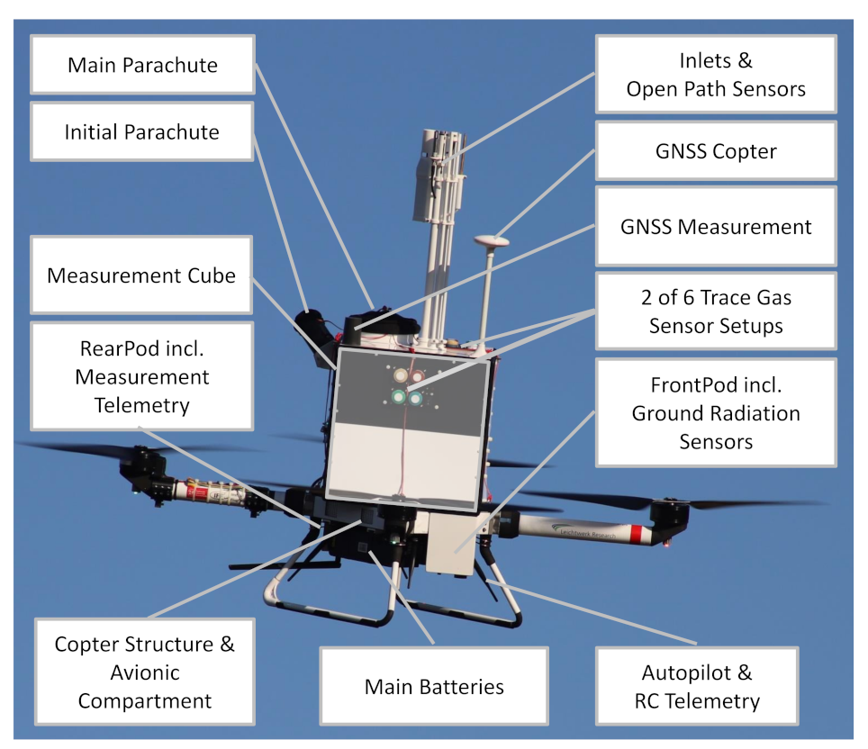
3. Multicopter System MesSBAR

The multicopter system MesSBAR is built up in a modular way. The different components are shown in Figure 2: The multicopter structure and avionics compartment constitute the central part of the system, where the rotor arms and other parts are attached. The main batteries for empowering the system are integrated below the central plate. The telemetry antennas for autopilot and remote control (RC) are attached downwards to the operator and ground station. The Front Pod contains sensors for characterizing the surface (pyranometer for solar reflected radiation and surface temperature sensor). The Rear Pod contains the telemetry antenna for the real-time data link to the ground control station. In the Measurement Cube the main sensors are integrated, namely, the POM, one ECS, the OPSS and the MA200. Up to four additional ECSs are attached to the sides and on the top of the Measurement Cube. For redundancy, there are two antennas for receiving and storing Global Navigation Satellite System (GNSS) data, one for the navigation and one for the measurements, which are directed upwards on top of the Measurement Cube. An emergency parachute is included for the case of loss of control, with a smaller initial parachute that can be activated either by remote control or the ground station, which pulls out the main parachute. On top of the multicopter are the open path sensors and the inlets for the aerosol and trace gas sensors.

3.1. Copter System

Based on the mentioned requirements, the multicopter systems MesSBAR were designed and manufactured. The final system has the following technical specifications:
The dimensions are a length/width of 16,543 mm and a height of 343 mm; the height including payload is 1137 mm. The maximum take-off weight is 25 kg due to current drone regulations, which make obtaining permission for systems with a weight exceeding this limit more difficult. The empty weight of the system is about 10.6 kg. Therefore, up to around 14.4 kg of payload including batteries can be attached. The material of the body is carbon-fibre-reinforced plastic (CFRP), glass-pearls-reinforced Polyamid (PA 12) and aluminum for joining elements.
The electric motor P80 III KV100 (T-Motor, Nanchang, China) is used together with propeller blades CF-PROP G30x10.5 (T-Motor, Nanchang, China). The rotor diameter amounts to 30’ (762 mm) with a rotor pitch of 10.5’. The maximum power output per engine is 2700 W (applicable for 180 s) at a voltage of 44.4 V. In the MesSBAR configuration, the electric accumulators are two lithium polymer batteries of type Tattu-23000mAh-22.8V-25C-6S1P (Grepow Electronics Co., Limited, Shenzhen, China).
The core of the flight system is a Pixhawk 2.1 autopilot system (CubePilot Pty Ltd. (Victoria, Australia)). This autopilot hardware, also named the “Cube flight controller”, is used in the Cube Orange version for the flight control of the MesSBAR copter. It is a flight controller with three redundant inertial measurement units (IMUs) for attitude and motion control. The quality of the IMU data is enhanced by temperature compensation and by mechanical decoupling from the rest of the flight system. The integrated Automatic Dependent Surveillance-Broadcast (ADS-B) for detecting airspace participants such as airplanes and helicopters in the surrounding area is not used, caused by the CFRP structure around. However, an additional external ADS-B receiver pingRX (uAvionics, Bigfork, MT, USA) is integrated. For MesSBAR, in addition to the assemblies essential for flight such as propulsion and radio modules, the parachute rescue system Safetech ST160 (Opale Parachutes, Marquise, France) with an area of 15 m 2 and a global navigation satellite system (GNSS) receiver are connected to the autopilot system. This GNSS receiver “GNSS2” (Zubax Robotics, Estonia) uses data from various satellite systems for a three-dimensional position calculation and utilizes a precise barometer for altitude estimation. An integrated three-axis compass detects the Earth’s magnetic field and uses it to determine the orientation and attitude of the copter. In addition to manual control, the autopilot system enables automatic flight of various flight profiles created in advance by the Mission Planner software from ArduPilot (ardupilot.org).
The ascent speed is up to 10 m·s 1 , and the descent speed is up to 2.5 m·s 1 . The flight endurance is limited by the batteries and allows a flight time of around 15 min.
The MesSBAR systems is designed and tested up to a take-off/landing wind speed of 10 m·s 1 and for a temperature range of 0 C to 40 C. The system has not been designed to be operated during precipitation, thunderstorms, icing conditions or other unusual weather conditions. The system is designed to operate by safety pilot and a operator supporting the monitoring and control of the autopilot system.

3.2. Sensor Integration
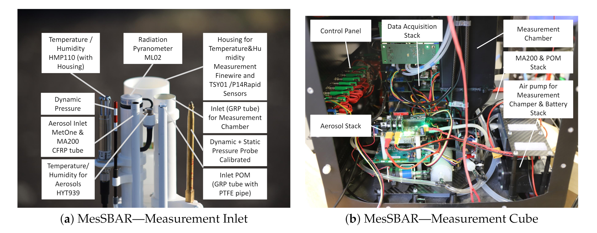
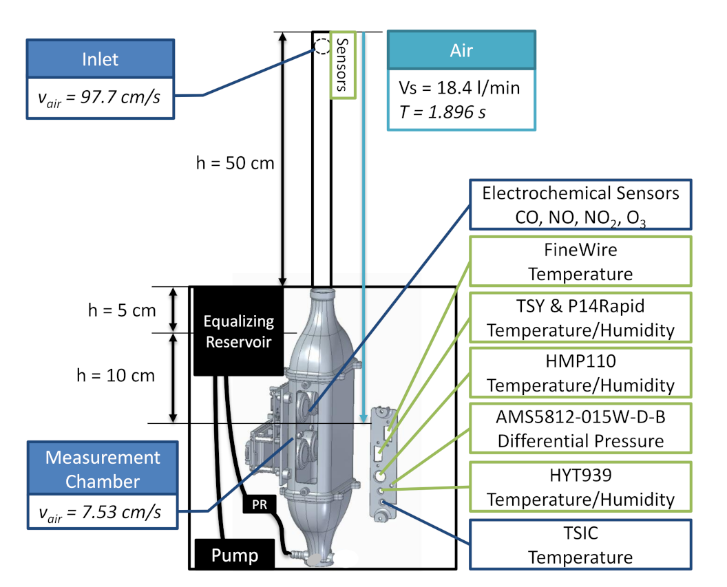
As shown in Figure 2, the inlets (see Section 3.2.1) collect the air and transport it to the measurement cube (see Section 3.2.2) and the included sensors, namely, the OPSS and MA200 (see Section 3.2.3), for aerosol measurements, and to the POM and to the measurement chamber (see Section 3.2.4) for the trace gas measurements, including one EC sensor stack (see Section 3.2.5). For validating the aerosol and trace gas measurements, Table 1 shows the integrated basic meteorological sensors. Slow sampling temperature/humidity sensors such as HMP100 and HYT939 are supplemented by fast sampling finewire and TSYS01/P14 Rapid sensors for the initial system verification. Those sensors are duplicated and disposed to the inlet and the measurement chamber to characterize the measurements in more detail. Temperature-compensated pressure sensors of type AMS5812, upward- and downward-looking pyranometers ML-02, an RGB-camera, an infrared (IR) objective temperature sensor MLX90614 as well as temperature sensors distributed in the Measurement Cube are implemented to document measurement conditions.

3.2.1. Inlet

Figure 3a provides a closer view of the sophisticated inlet. The inlet consists of four tubes joined together. Because of the tube length of 500 mm, the mounting of the tubes is realized as a rated break point to ensure a safe expansion of the parachute. An Acrylnitril–Butadien–Styrol–Copolymer (ABS) 3D-printed mounting fixes the tubes with 3 M4 nylon screws to the top of the Measurement Cube. A 20 mm tube made of glass-fibre reinforced polymers (GRP) contains all sensor cables and pipes. On top of this tube, the upward-looking ML02 pyranometer for measuring solar radiation is mounted. The second 20 mm GRP tube is used as an inlet for the measurement chamber and its trace gas sensors. Both tubes are made of GRP to reduce the impact to the GNSS receiver while ensuring an light and stiff structure. The first 6 mm tube is a joint inlet made of CFRP for OPSS and MA200.
In the copter versions P and OPv.1, the aerosol is sampled with a total flow of 3 L min 1 , resulting in a Reynolds number of 708 indicating laminar flow. The length of the inlet in version P is 78 cm and in version OPv.1 53 cm. The upper cut-off size of the inlet strongly depends on the horizontal wind speed and orientation of the copter, which does not allow for a precise determination of this value. Therefore, the upper measurement limit is assumed to be 10 μ m , which corresponds to the observable diameter range of the OPSS given by the manufacturer. As an example, an upper cut-off of 10 μ m is given for a particle density of 2 g cm 3 and horizontal wind of 1.68 m·s 1 . In the first operational version (OPv.1) and the prototype version (P) of MesSBAR, the optical cell of the OPSS is centered below and directly connected to the inlet to avoid bends. The CFRP ensures conductivity.
In MesSBAR versions OP v.1 and P, the sample flow of the MA200 is collected with a stainless-steel tube with a 1.9 mm outer diameter located in the core-flow of the main inlet. A custom Nafion-membrane dryer dries the sample stream of the MA200 and also dampens gradients of the sampling RH, which can cause significant bias in the MA200 readouts (e.g., [44]). The needed counter flow is provided via dried excess air of the OPSS pump dried with silica.
The second 6 mm tube is a CFRP tube and includes a PFA pipe as an inlet for the POM. In addition to the tubes, the inlet is equipped with temperature and humidity sensors: the HMP110 with the housing provided by the manufacturer, a HYT939 sensor for aerosol measurements as well as a combination of our own developed electronics boards with our own housings (fine wire temperature sensor, temperature sensor TSY01 and capacitive humidity sensor Rapid P14) for fast response measurements. Furthermore, in copter version P, two probes are mounted to the tubes to compare dynamic pressure measurement.

3.2.2. Measurement Cube

A detailed view on the Measurement Cube is provided in Figure 3b. The measurement technique is organised in different modular stacks that can be combined flexibly: There are stacks for the OPSS, the MA200 and the POM. There is a separate stack for the air pump sucking the air through the inlets and then the measurement chamber, and the battery for operating the measurement technique. The battery is not needed within the operational version by moving the power consumption to the main batteries. Furthermore, there is the data-acquisition stack (see Section 3.3). The control panel provides information on the status of the different systems (power, GNSS reception and recording state) that is easily visible to the operator. It contains switches and circuit breakers for switching the power supply on and off and starting the data recording.

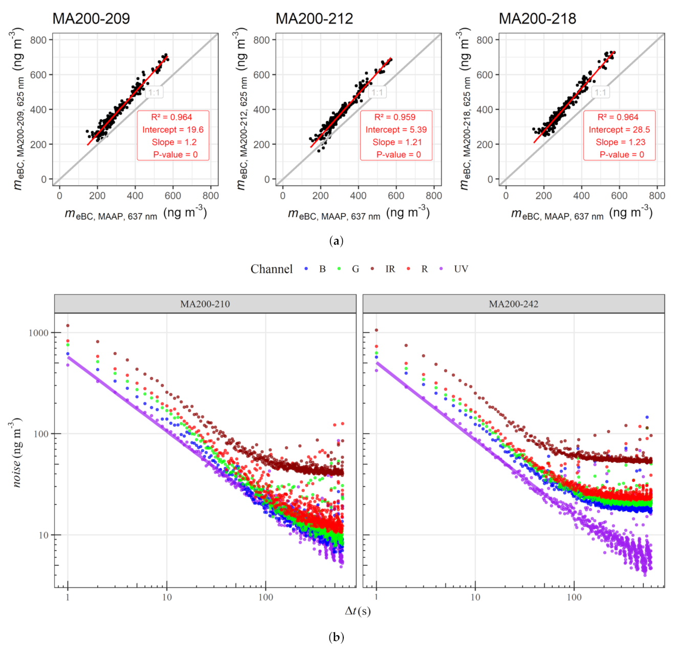
3.2.3. Aerosol Measurements

The MA200 probes the equivalent black carbon (eBC [45]) mass concentration ( m e B C ). Advantageously, the MA200 senses at 5 wavelengths (375, 470, 528, 625 and 880 nm). Its applicability has been proven in mobile measurements such as exposure studies (e.g., [36,46]). However, measurements revealed a distinct dependence of the readouts on temperature and RH changes especially at 375 and 880 nm. For wavelengths larger than 600 nm, the contribution to aerosol particle light absorption of organic carbon (OC) is small with low MACs [47]. Hence, meBC is derived at 625 nm. The uncertainty induced by noise is characterized for the five channels of the MA200 in terms of the averaging period with filtered air (see Figure 1b).
The OPSS operates at six nominal size channels. On the manufacturer’s side, the device is calibrated with spherical polystyrene latex (PSL) particles of a given refractive index (1.59 + i0) and diameter. This calibration leads to uncertainty when applied to real-world aerosols with differing shapes, sizes and refractive indices. Hence, the PSL-equivalent size bins have to be transformed to fit ambient aerosol utilizing a refractive index of 1.54 + i0, which resulted into a good overlap with refractive-index-independent reference instrumentation and is in the range of the refractive indices used in [36]. The upper and lower diameters, as well as the geometric mean diameter, of the size bins determined for the PSL refractive index and the assumed refractive index are given in Table 2. The manufacturer states a measurement uncertainty of 10%. The OPSS was already successfully used in previous studies (e.g., [4]). The OPSS operates at a target volume flow of 2.83 L min 1 (0.1 cfm). Unfortunately, the instrument does not report the sample flow rate, which is addressed as described in Section 3.2.3.
The aerosol instrumentation on MesSBAR is implemented with the following sensors listed in Table 3.
The OPSS is disassembled, and the battery, housing and display are removed. The printed circuit board (PCB) of the OPSS, its pump, a silica-bead-based dryer and a mass flow meter (MFM; mod. SFM4100, Sensirion) are integrated in a stack also containing a PCB responsible for data acquisition and processing, parameter observation and flow control. Data acquisition, processing and pump control are handled by the Teensy® 3.6 development board. The sample volume flow is controlled via a feedback-based PID (proportional–integral–derivative) control loop mechanism in which real-time data of the pressure (from BME 280 sensor on board the PCB), mass flow (non-temperature compensated) and temperature are utilized. The sample RH downstream of the dryer is observed with an RH-/T-sensor (mod. HYT-939, IST-AG, Ebnat-Kappel, Switzerland).

3.2.4. Measurement Chamber

The measurement chamber is designed and implemented to obtain controlled air flow conditions and prevent the impact of solar radiation on the trace gas sensors.
Figure 4 illustrates the implementation of the measurement chamber and the related components. The 20 mm CFRP tube that is mounted on top of the Measurement Cube delegates the air to the 3D-printed ABS chamber. The chamber continuously slows down the air as a result of the needed inner size to integrate the electrochemical sensor stack (explained in Section 3.2.5) and the meteorological sensors fixed on the side plate. The meteorological sensors are also illustrated in Figure 4 by showing the holes in the side plate for each listed sensor. Therefore, the duplicated sensors compared to the inlet enable a comparison between the open path and closed path conditions. Furthermore the outgoing flow system, with its Pressure Reducer (PR), the equalizing reservoir and the 3KQ series diaphragm pump (575 g, Boxer GmbH, Ottobeuren, Germany), provides a constant flow rate of 20 L min 1 through the measurement chamber, which constitutes a laminar flow with a Reynolds number Re ≈ 320).
For that outgoing flow system, a separate investigation was needed because the first setup that directly connected the pump to the 4 outlets on the bottom of the measurement chamber showed a conspicuous pressure oscillations with an amplitude of ±275 Pa. By having a maximum expected range at standard conditions between −3 Pa (maximum sink rate 2 m/s) and 15 Pa (operation climb rate 5 m/s) and 100 Pa at maximum climb rate of 10 m/s, the measured ±275 Pa oscillations are too much for the pressure measurements.
Therefore, the flow rate was measured with the SFM3000-200-C (Sensirion, Switzerland) installed at the inlet. Regarding the required air flow speed in the chamber of 5 cm/s for the electrochemical sensors, the estimated flow rate limit is 12.15 L/min. The pressure was measured with the already installed AMS5812-015W-D-B, as well as a Kulite XT190 (Kulite Semiconductor Products, Inc., Leonia, NJ, USA).
First, the use of a PR between the pump and chamber has to be evaluated by reducing the pipe diameter with pliers while monitoring and recording the flow and pressure. Figure 5a shows the pressure oscillations in Pa over time. With the reduction in the cross-section, the pressure oscillation can be reduced to ±17 Pa while the flow rate also reduces greatly down to 12.5 L/min. The next approach was to use an equalizing reservoir. Several reservoirs were evaluated, starting with a hard plastic 1 L PET bottle, using soft plastic 1 L PET bottle, cascading 2 bottles, using a quadratic 1 L bin made of Polyvinyl-alcohol (PVA) profiles and a thin plastic sheet ending up in a CFRP reservoir made of thin CFRP sheets and CFRP L-profiles. The investigation showed that the reservoir reduces the flow rate from 23 L min for the initial setup down to 19.5 L min on average. The bottles reduced the pressure oscillations from ±275 Pa down to ±17 Pa. The different materials show less influence. By increasing the bottle volume to 2 L the pressure oscillation is reduced to ±14 Pa, but other than that, a 2 L reservoir is too big and cannot be integrated within the designed cube. However, the quadratic reservoirs with their flexible skin reduced the pressure oscillation down to ±7.5 Pa. Finally, Figure 5b shows the combination of the final 1 L CFRP reservoir and the manual pressure reduction while reducing the flow rate. The trend shows a leveling at ±3 Pa, meaning a further change in the cross-section will not reduce the pressure oscillation that much.
From these results, a constant pressure reducer is built reducing the inner diameter to 3 mm. In combination with the CFRP reservoir, a flow rate of 18.4 L min 1 and a pressure oscillation of ±4 Pa is measured and considered as an appropriate value for the measurement chamber characteristic.

3.2.5. Trace Gas Measurements

Reactive trace gases are measured by means of electrochemical sensor setups and a Personal Ozone Monitor (POM, 2B Technologies) shown in Table 4. Up to six trace gas sensor setups have been installed on the drone: one on each side panel, one on top and one connected to the dedicated measurement chamber maintaining a constant laminar sampling flow across the sensors. All single-sensor setups have a power supply as well as an interface to the centralized data-acquisition system. Each setup consists of four electrochemical sensors (Alphasense; CO-B4, NO-B4, NO2-B43F, Ox-B431), a Telaire ChipCap 2 sensor for temperature and relative humidity measurements and a circuit board to manage and store incoming data at a frequency of 1 Hz. The individual components are mounted on a 3D-printed carrier plate and can be exchanged easily for post-flight calibration. To realize an uninterrupted power supply (e.g., in case of an exchange of the main measurement batteries between flights), two additional batteries are used for each setup. The total weight of 1 setup is around 250 g.
The POM uses the absorption of UV light at 254 nm to detect ozone (Federal Equivalent Method, FEM). With dimensions of 14.0 × 7.6 × 3.8 cm, a weight of 360 g and a low power consumption of 3.0 W, it is well-suited for UAS measurements. The POM actively samples air at a flow rate of 0.8 L min 1 through a 0.8 m long perfluoroalkoxy alkane (PFA) line from the inlet (see Section 3.2.1). The time resolution is 2 s with a limit of detection of 3.0 ppb (2 σ ).

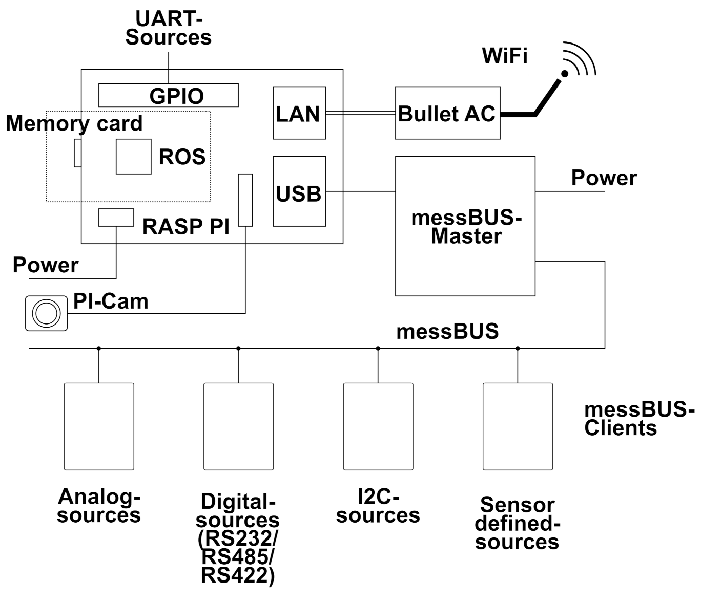
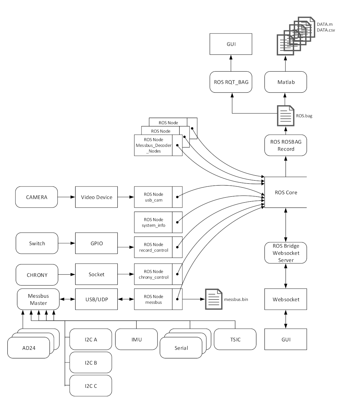
3.3. Data Acquisition and Management

A data acquisition system developed at the IFF consisting of a single board computer, a data transmission system between several participants, called messBUS (mB), and the logging software brings together all the data sources. Consistent time stamps are generated, and the acquired measured values are synchronized with them. The acquired data are then stored on a memory card. The single-board computer can be accessed via WiFi to display important parameters and current measurement results. Figure 6 shows a schematic diagram of the data-acquisition process.
At the center of the data acquisition is a Raspberry Pi (RASP PI) 4 Model B with 8 GB random access memory (RAM) (Raspberry Pi Foundation, United Kingdom). The single-board computer works with an Ubuntu operating system and provides various digital interfaces. Via the dual-band AirMAX(R) AC radio Bullet-ac from Ubiquiti Networks (New York, NY, USA), a stable WiFi connection can be established, and bidirectional communication with a ground station is enabled. The WiFi connection is used in in-flight telemetry and post-flight data log access. In addition to the RASP PI’s integrated camera interface, general purpose input/output (GPIO) pins are used for universal asynchronous receiver transmitter (UART) communication. This is used to acquire data from the Pixhawk autopilot system and the meteorology GNSS receiver. Since the measurement system consists of a variety of different measurement devices and sensors, the mB is used for data acquisition. The mB is able to use different data sources. It consists of two modules, the mB master and a defined number of mB clients. This mB system is developed and manufactured by the Institute of Flight Guidance of TU Braunschweig and the company messWERK GmbH. The mB master communicates via a user datagram protocol (UPD) stream with the universal serial bus (USB) interface of the connected computer (Figure 6). For synchronization, the mB master uses the pulse per second (PPS) signal of the meteorology GNSS receiver. With this time base, the mB clock is defined and readjusted. Furthermore, a consistent time stamp can be generated from it. In addition to the computer connection and synchronization, the mB master controls the communication on the messBUS. For this purpose, the mB master queries the messBUS for participants (mB clients) and generates the required transmission time of the individual participants from the messages received. From this information, the mB occupancy is created. Each registered client receives a certain time and a certain time span, that is, when and for how long this can occupy the messBUS. The process is repeated every 10 ms and enables the polling of all BUS participants with 100 Hz. The messBUS clients are the interfaces to the measuring devices and sensors. MessBUS clients enable communication with different data sources and thus have a specific function. This is shown in the lower part of Figure 6. There are clients for analog signals, digital communication protocols such as I2C, RS232 and RS485/422 and for special sensors. In Table 1, the “Interface” column shows the path used to collect data from each source. Data sources are defined as all devices that generate measured values. These include the sensors for temperature, relative humidity, pressure, position, radiation, the aerosol stack, the POM handheld ozone meter, the electrochemical sensor boards, the Pixhawk autopilot system, the camera and the GNSS receiver. The data of the measuring systems described in Section 3.2.3 and Section 3.2.5 are transferred to the messBUS via RS232 interfaces and recorded by MessBUS clients.
Within the Ubuntu operating system, the Roboter Operating System (ROS) in the version “Melodic Morenia” is used as a centralized data management system. Figure 7 illustrates the interfaces that are addressed and read out individually. ROS nodes are used to publish the input data within the ROS core. Decoder nodes subscribe to the raw input data messages and decode and publish them again. The published data are accessed via a websocket connection for a near-real-time telemetry on the ground station. Furthermore, the published data are recorded within a ros.bag on an SD card. It is used for the post-flight analysis by the use of python and matlab routines. Those routines filter, calibrate and synchronise data in time. Afterwards the data are exported for the EURAD-IM simulations, a quality control and a publication in public clouds (e.g., mCLOUD).

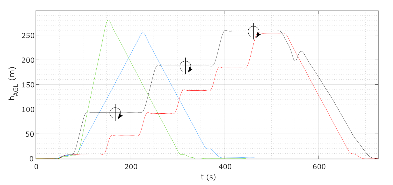
4. First Applications
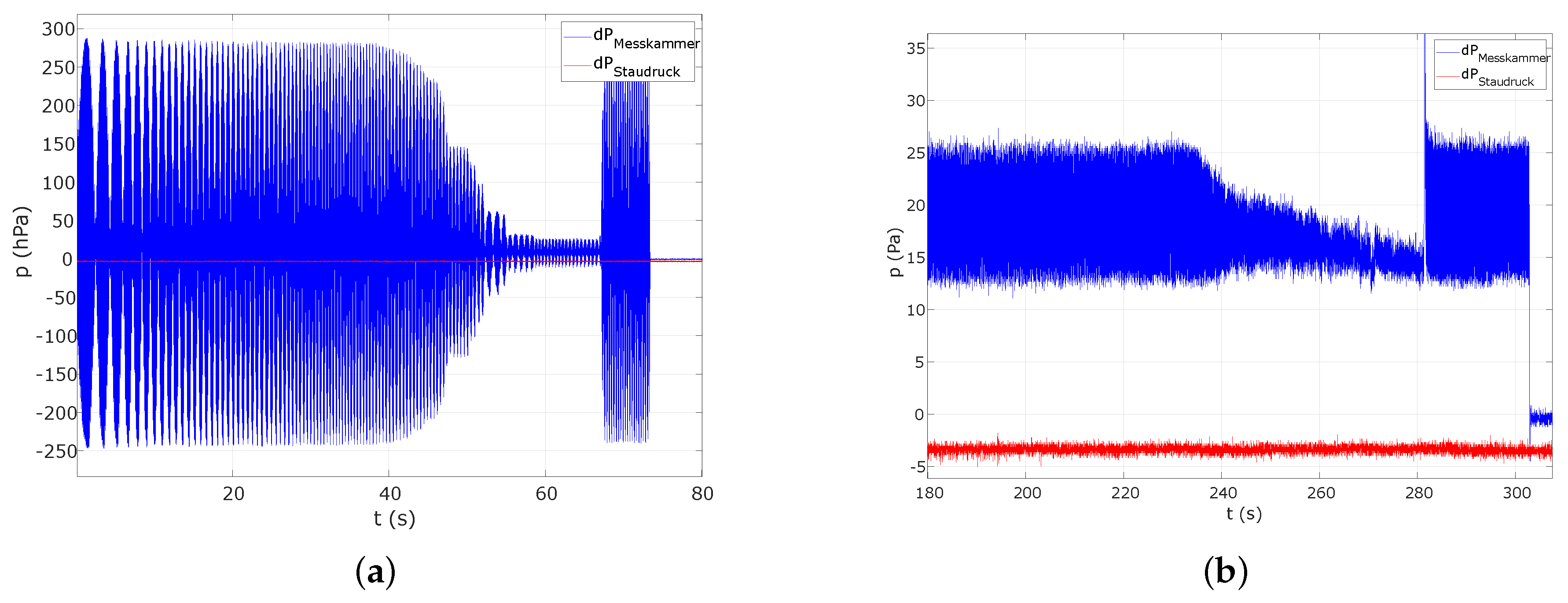
The first application of the technical tested measurement system took place in Wesseling, Germany (50 47 28.7 N, 7 00 22.9 E). System version P was flown at the “Wesseling I” campaign for the first time. Fifteen flights have been performed (Table 5). The campaign’s objective was to obtain a first complete data set to characterize the sensor system as well as the copter. The “Wesseling II” campaign with its 20 flights (Table 5) included a detailed data analysis, and copter version OP v.1 was operated. The objective was to fly during the morning transition within and above the boundary layer to obtain more information about the response characteristics of the aerosol and trace gas sensors. Furthermore, the EURAD-IM simulations were taken into account for the planning as well as in the post-campaign analysis.
For sensor comparison the pollution observation station operated by the Federal Highway Research Institute (BASt—Bundesanstalt für Straßenwesen) at around 200 m distance to the highway A555 near Wesseling, Germany were used. The BASt station is equipped with instrumentation to observe the mass concentration of gases, PM and eBC. An OPSS (mod. Fidas® 200, PALAS GmbH, Karlsruhe, Germany) observes PM 1 , PM 2.5 (10.8% uncertainty; 1.06 linearity), PM 4 , PM 1 0 (7.8% uncertainty; 1.03 linearity) and the total suspended particulate matter PM t o t . This allows real-time comparison with the MesSBAR measurements. An Aethalometer® (mod. AE33, Magee Scientific, Berkeley, CA, USA) derives the m eBC at 880 nm, and its data are harmonized to a MAAP with a harmonization factor of 1.76 based on European-wide ACTRIS measurements.
In both campaigns, vertical profiles up to 280 m above ground level were conducted during the day time. Table 5 lists the flown mission profiles over the days. Figure 8 illustrates four typical profiles. The blue (continuous 1 m/s ascent) and the red (6 times 1 min steps, 4 m/s ascent in between) profiles were executed as standard double profiles for 3 or more times consecutively. The green profile in Figure 8 with its 5 m/s ascent illustrates the continuous profiles with different vertical speeds and the resulting influences on the sensors that were investigated. The data showed that for the given system, an ascent rate of 3 m/s was the limit where the ram pressure influenced the inflow significantly, specially in the measurement chamber. The black profile in Figure 8, with a 4 m/s ascent and a 2 min hover, including a 180 degree turn in direction after 1 min, was used to obtain the known effects of the radiation to the ECS setups and the inlet system. The effect of the 50 cm inlet in the P version was the reason why we investigated the shortened 0.25 cm inlet tubes in the OPv.1 version. Finally, the influence of thermal radiation was reduced. While the step-wise profiling showed disadvantages with its pressure changes after the ascent phases and the needed adaption phase at the beginning of the single steps, the continuous profiles are preferred for the upcoming campaigns. For that reason, Table 6 lists 9 continuous vertical profiles of 24 measurements at Wesseling II that are investigated and explained in the following.

4.1. Basic Air Data

The two days of operation were characterized by no clouds and low surface wind from southeast directions on 22 September and more from south to west on 23 September. The motor way has a direction of 155°/335°. Hence, the effective east component was larger on 22 September and emissions from the highway were probably sampled by the drone, whereas, on 23 September, they were most likely not.
On 22 September 2021, the potential temperature near the surface increased from 278 K during the first flight at 05:00 UTC (07:00 local time) to 292 K (Figure 9a). At the beginning of the measurement period, the atmosphere was stably stratified with increasing potential temperature with altitude. During Flight 5 at 8:00 UTC, a mixed layer with constant potential temperature was observed up to an altitude of 125 m. During Flight 7 at 9:30 UTC, the mixed layer extended up to an altitude of 220 m. During Flight 9, the temperature inversion was at higher altitudes than sampled with the copter. The development of stratification is also visible in the profiles of relative humidity: Overall the relative humidity decreases during the flight period. Furthermore, it decreases above the altitude of the temperature inversion. The solar energy increased constantly from flight 1 with approximately 0 W/ 2 to flight 8 with a maximum solar radiation of 850 W/m 2 . Then, it was constant with less influences of clouds and decreased from flight 10 to the end of day I.
On 23 September 2021, the near-surface temperature increase was more unstable due to the clouds, from 280 K at 05:05 UTC to 297 K at 11:22 UTC. Clouds reduced the solar radiation between flight 1 (05:05 UTC) and 7 (08:32 UTC). Afterwards, the clouds decreased. During the measurement period, the ground-base temperature inversion did not dissolve. The relative humidity was enhanced up to an altitude of 75 m at the beginning but decreased with time. The two contrasting situations concerning atmospheric stability had an impact on aerosol and gas measurement.

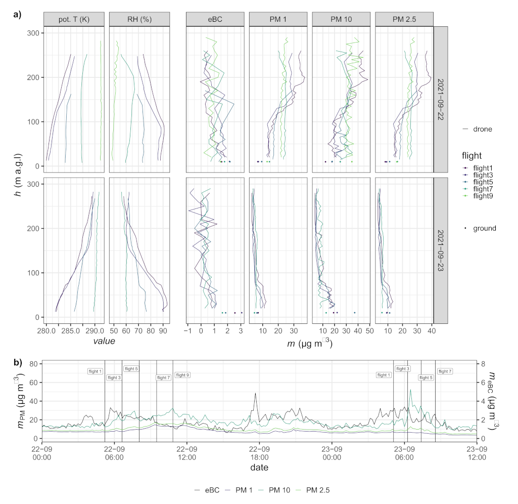
4.2. Aerosol Measurements

The vertical profiles (Table 6) are selected filtering for ascending speeds ( v asc 0.9 m s 1 ) and an altitude above ground was arbitrarily chosen to be larger than 10 m to prevent influence by the rotor down wash during MesSBAR’s start and landing. The mean time (UTC) of the vertical profiles is displayed in Table 6, where flight 9 on 22 September and flight 7 on 23 September contain two vertical profiles.
Figure 9b displays the mass concentration over time for PM and eBC. The daily commuting traffic cycle on the motor way is visible in the eBC mass concentration evolution over time with three distinct peaks during the shown period at around 6:00 a.m. and 6:00 p.m. UTC. In the morning peaks, the vertical profiles were conducted.
On 22 September 2021, 2 distinct layers separated at around 125 m altitude were observed, indicated by a slight change in the gradient of the potential temperature and by a sharp decrease in the RH at this altitude. During the first flight, in the upper layer, a PM 10 mass concentration of about 50 μ g m 3 can be seen, which is about 3 times higher than in the layer below. Due to boundary layer development, the lower layer increases in thickness in the course of the day, and separation could not be observed anymore during flight 9. While this layer is growing in thickness, the mass concentration of particulate matter decreases due to dilution. The mass concentrations of PM 1 and PM 2.5 show a similar pattern but with different magnitudes. meBC behaves oppositely, decreasing during the first flight, from the ground level to higher altitudes, and reaches a rather stable concentration along height at around 1 μ g m 3 observed during flight 9.
On 23 September 2021, there was an opposite layering observed. During the first 3 flights, below an 80 m altitude (above ground), most of the particulate matter was trapped with around twice as large mass concentrations in PM 10 of around 15 to 20 μ g cm 3 . In the course of the day, the stable layering weakens due to heating by solar radiation and becomes more neutral, allowing for a particulate matter exchange with higher altitudes.
Opposite to PM, m eBC decreases with altitude during the first flights on both days and is more or less constant over the entire observed altitude range in the last flights of the campaign.
Figure 9a displays the corresponding ground measurements of PM 1 , PM 2.5 , PM 10 and eBC as dots with corresponding colors.
On 22 September 2021, MesSBAR derived PM 1 (PM 2.5 ; PM 10 ) values in the 10 m layer (10 to 15 m) corresponding to 0.47 to 0.61 (0.52 to 0.68; 0.57 to 1.17) times the values derived by the OPSS at the ground station. For 23 September 2021, the factors for PM 1 (PM 2.5 ; PM 10 ) are 0.64 to 0.82 (0.78 to 1.14; 1.16 to 2.32). PM 1 and PM 2.5 , however, are within a reasonable range compared to the measurements at ground level on 22 September. These difference could be for manifold reasons, e.g., the assumed aerosol density, the volume correction factor for PM 1 or the PM-readouts of the reference station on the ground could be too small, since these are also based on empirical measurements [48]. Moreover, on 22 September, a much larger aerosol load is observed and could be explained by a larger coarse mode of the aerosol. Since the MA200 samples the aerosol in the core flow of the inlet, here, sedimentation losses could cause an under-sampling of larger particles. However, because of the limitation to 6 size bins, these results are promising and show the applicability of the method used here.
For eBC (layer from 10 to 20 m), factors of 0.87 to 2.04 on 22 September are derived. On 23 September, m eBC measured by the MA200 is a factor of 2.24 to 5.75 smaller compared to the AE33 at BaSt station and is significantly smaller than on the previous day. Here, differences could be explain by different wind direction observed at both days. Whereas, on 22 September, the MesSBAR was operating downwind of the highway (mean wind direction 160° and motor way in 30° direction); the east component (downwind) was smaller on 23 September with a mean wind direction of 175°, so that MesSBAR was less influenced by the direct emissions of the highway.

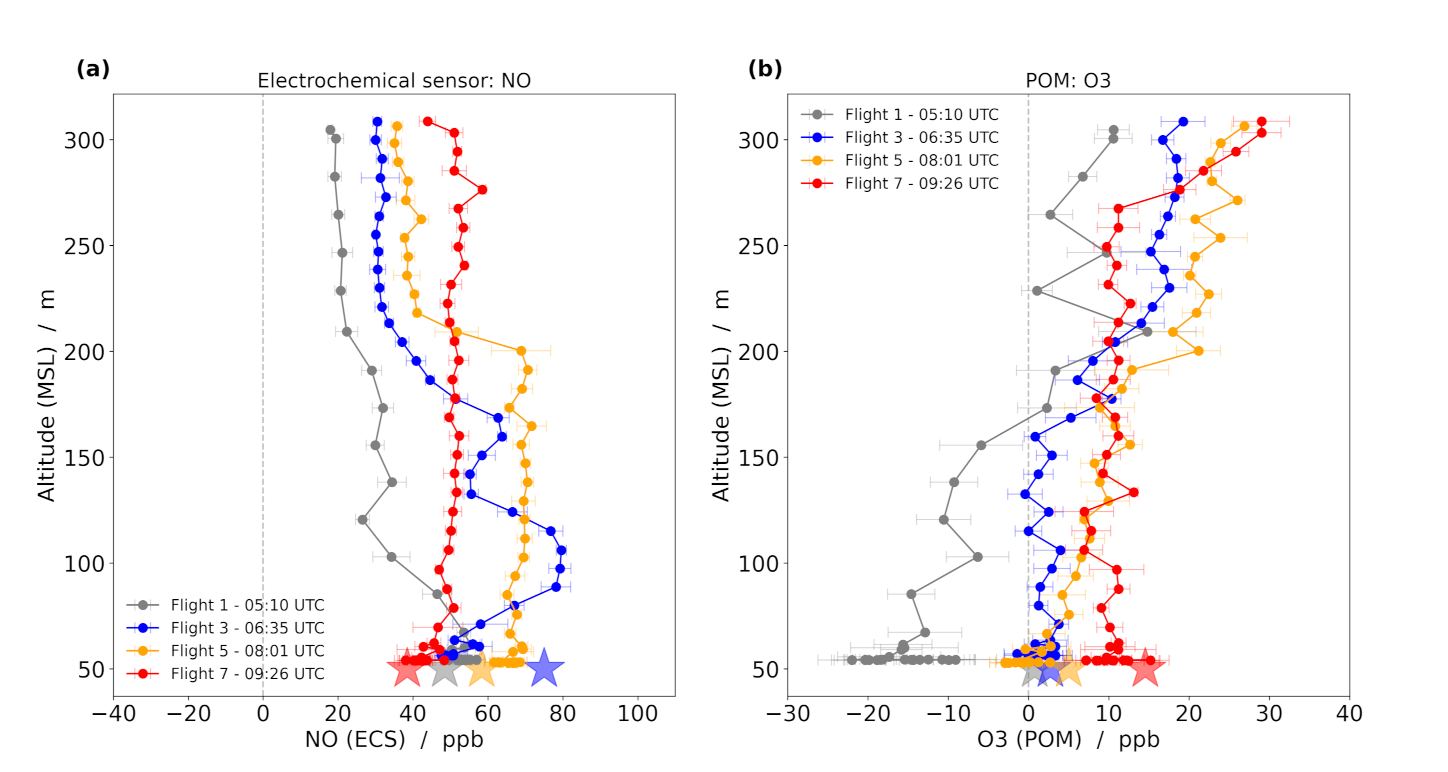
4.3. Reactive Trace Gases

Figure 10 shows the vertical profiles of NO (NO-B4) and O 3 (POM) measured downwind the motorway at Day I. Data points are averaged to 10 s intervals with their standard deviations included as error bars. The values are compared to the mean mole fraction obtained from a ground-based measurement station situated on the same side of the motorway where the flights took place (indicated by stars). Good agreement was found between the ground station measurements and the UAS system data on the ground. There are only two exceptions: NO at flight 3 started at lower values but increased to the corresponding mole fraction at the ground after about 40 m, and O 3 at Flight 1 showed an offset possibly attributed to a too-short warm-up period of the POM.
The morning evolution (see temperature in Figure 9a) of the planetary boundary layer height at Flights 1, 3, 5 and 7 can be seen in elevated NO and lowered O 3 mole fractions at low altitudes. The thickness (altitude) of these layers increases with time until the lower layer is well mixed within the flight altitude of the drone (flight 7).
The high NO mole fraction at the beginning results from ground-based emissions from cars and trucks: These are accumulated near the ground due to the early morning temperature inversion. Increasing solar radiation leads to increased vertical mixing due to convection. As a result, the NO mole fraction decreases near the ground and increases at higher altitudes until a nearly constant profile is obtained (Flight 7). Ozone (Figure 10b) shows a vertical profile opposite to NO (Figure 10a) due to their reaction forming NO 2 . The NO emissions from the traffic source keep the ozone mole fractions near the ground low, and the formation of NO 2 is limited by the photo-chemically induced ozone production.
The measurements show that the sensors provide very good results by means of a constant ascent speed that is as slow as possible. This is especially important for the externally mounted setups to realize a flow as uniform as possible over the sensors. Therefore, this is a trade-off between possible altitude and flight speed with respect to the power capacity. Further measurement campaigns will provide further insights on the optimum ratio of these parameters in relation to the sensor’s measurement accuracy. Within MesSBAR is no reference device for the electrochemical sensors in the air, but there is a good agreement between the sensors (Figure 10) and the devices in the measuring container on the ground (shown with stars). An in-flight comparison of the electrochemical sensors with a reference device was performed by using a Zeppelin NT [34]. The insights of these results have the possibility to further improve the UAV measurements, and the included laboratory calibration procedure in the future since the Zeppelin NT and the MesSBAR UAS have similar flight characteristics (speed, altitude).

5. Conclusions

Overall, the MesSBAR measurement system is a further step towards high-resolution vertical air quality measurements. The first applications show the large potential of the system. By starting with a extensive sensor setup within both campaigns as well as with the pre- and postflight investigations, a lot of information about the system and its application could be achieved. It will result in the operational version 2, where an improved power management, a reduced number of basic meteorological sensors, an advanced measurement temperature control as well as an easier handling will be integrated.
In terms of the aerosol measurements, the first results are promising, and the overall flight pattern was suitable to observe shallow planetary boundary layers. However, for the future, more measurements are needed especially for conditions of larger particles to ensure the applicability of the utilized method as well. To reduce losses, the inlet system for MesSBAR (OP v.2) will be revised and the sampling of the MA200 will collect the aerosol downstream of the optical cell of the OPSS.
For online quality assurance, a ground-station equipped with instrumentation identical to the devices on board of MesSBAR would allow a field quality check by near-real-time comparison. Furthermore, the direct contribution of the pollutant source can only be quantified by parallel conducted measurements with two identical multicopters upwind and downwind of the emission source.
The first field results are promising in terms of trace gas measurements, based on the agreement between the drone and container measurements on the ground as well as on the vertical NO and O 3 profiles. With these profiles, the evolution of the morning planetary boundary layer height was detected. However, detailed investigations are needed to find the right balance between possible altitude and flight speed in terms of power capacity to achieve the best spatio-temporal resolution. Continuous vertical ascents provided better measurement conditions than the originally planned step profiles with phases of hovering.
The quality of the electrochemical sensor data relies heavily on the calibration method. Therefore, the knowledge gained from the performed UAV flights in combination with measurements on board a Zeppelin NT will be used for further improvements in the electrochemical sensor calibrations by simulating the flight conditions in the laboratory.
The use of the presented multicopter allows us to complement the classical ground-based observations with information on the vertical distribution of the pollutants, which is strongly linked to atmospheric properties, in particular, stability. The flexible methodology provides a significant improvement in determining the vertical distribution of pollutants compared to other techniques, such as the deployment of towers [49], tethered balloon systems [50] or Zeppelins [34].
Also for inverse modelling applications, the first observation results seem promising. Receiving detailed profiles of diverse pollutants simultaneously as input data for the 4d-var data assimilation algorithm offers great potential, especially for the optimisation of local emission sources with EURAD-IM. A significant information gain due to additional UAS measurements is expected compared to assimilating ground-based observations only. Accordingly, detailed analyses of the observability of UAS air quality measurements with respect to the representation of local plumes in the EURAD-IM will be part of future work.

Author Contributions

Development of project idea and funding acquisition, A.L., A.B., V.E., T.K., A.C.L., M.L., R.T. and B.W.; development of multicopter and payload, L.B., A.S. (Andreas Schlerf), S.D., P.F., R.K., F.P., H.S., T.S. and C.W.; field application, L.B., A.S. (Andreas Schlerf), A.B., M.B., S.D., T.K., P.F., H.S., F.P., J.R., R.S., A.S. (Andre Sobotta), T.S. and C.W.; preparation of pollution forecasts, H.E. and A.C.L.; development of laboratory calibration procedures, L.B., A.S. (Andreas Schlerf), S.D., V.E., H.B., J.S., A.N., F.P., T.S., R.T., B.W., C.W. and K.W.; writing—original draft preparation, L.B. and A.L. All authors contributed to reviewing and editing. All authors have read and agreed to the published version of the manuscript.

Funding

This work has been funded by the Modernity Fund (mFUND) of the Federal Ministry of Transport and Digital Infrastructure(BMVI) under grant agreement 19F2097A (MesSBAR—Automatisierte luftgestützte Messung der Schadstoff-Belastung in der erdnahen Atmosphäre in urbanen Räumen).

Institutional Review Board Statement

Not applicable.

Informed Consent Statement

Not applicable.

Data Availability Statement

Data collected with MesSBAR will be available at the cloudstorage of TU Braunschweig during the project. All data will be archived at the World Data Centre PANGAEA at the end of the project.

Acknowledgments

The authors would like to thank the students who were involved in the framework of a student thesis or as student research assistants: Deike Müseler, Dominik Hanke, Lennart Fox, Lukas Jäger, Lara Kuhr and Markus Kleinecke.

Conflicts of Interest

The authors declare no conflict of interest. The funders had no role in the design of the study; in the collection, analyses, or interpretation of data; in the writing of the manuscript, or in the decision to publish the results.

References

  1. Mayer, S.; Sandvik, A.; Jonassen, M.O.; Reuder, J. Atmospheric profiling with the UAS SUMO: A new perspective for the evaluation of fine-scale atmospheric models. Meteorol. Atmos. Phys. 2012, 116, 15–26. [Google Scholar] [CrossRef]
  2. Martin, S.; Beyrich, F.; Bange, J. Observing Entrainment Processes Using a Small Remotely Piloted Aircraft System: A Feasibility Study. Bound.-Layer Meteorol. 2014, 150, 449–467. [Google Scholar] [CrossRef]
  3. Jonassen, M.O.; Tisler, P.; Altstädter, B.; Scholtz, A.; Vihma, T.; Lampert, A.; König-Langlo, G.; Lüpkes, C. Application of remotely piloted aircraft systems in observing the atmospheric boundary layer over Antarctic sea ice in winter. Polar Res. 2015, 34, 25651. [Google Scholar] [CrossRef] [Green Version]
  4. Lampert, A.; Altstädter, B.; Bärfuss, K.; Bretschneider, L.; Sandgaard, J.; Lobitz, L.; Asmussen, M.; Damm, E.; Käthner, R.; Krüger, T.; et al. Unmanned Aerial Systems for Investigating the Polar Atmospheric Boundary Layer—Technical Challenges and Examples of Applications. Atmosphere 2020, 11, 416. [Google Scholar] [CrossRef] [Green Version]
  5. van den Kroonenberg, A.; Martin, S.; Beyrich, F.; Bange, J. Spatially-Averaged Temperature Structure Parameter Over a Heterogeneous Surface Measured by an Unmanned Aerial Vehicle. Boundary-Layer Meteorol. 2012, 142, 55–77. [Google Scholar] [CrossRef]
  6. Lampert, A.; Pätzold, F.; Jiménez, M.A.; Lobitz, L.; Martin, S.; Lohmann, G.; Canut, G.; Legain, D.; Bange, J.; Martínez-Villagrasa, D.; et al. A study of local turbulence and anisotropy during the afternoon and evening transition with an unmanned aerial system and mesoscale simulation. Atmos. Chem. Phys. 2016, 16, 8009–8021. [Google Scholar] [CrossRef] [Green Version]
  7. Wildmann, N.; Bernard, S.; Bange, J. Measuring the local wind field at an escarpment using small remotely-piloted aircraft. Renew. Energy 2017, 103, 613–619. [Google Scholar] [CrossRef]
  8. Altstädter, B.; Platis, A.; Wehner, B.; Scholtz, A.; Wildmann, N.; Hermann, M.; Käthner, R.; Baars, H.; Bange, J.; Lampert, A. ALADINA—An unmanned research aircraft for observing vertical and horizontal distributions of ultrafine particles within the atmospheric boundary layer. Atmos. Meas. Tech. 2015, 8, 1627–1639. [Google Scholar] [CrossRef] [Green Version]
  9. Platis, A.; Altstädter, B.; Wehner, B.; Wildmann, N.; Lampert, A.; Hermann, M.; Birmilli, W.; Bange, J. An observational Case Study of the Influence of Atmospheric Boundary-Layer Dynamics on New Particle Formation. Bound.-Layer Meteorol. 2015, 158, 67–92. [Google Scholar] [CrossRef]
  10. Villa, T.F.; Gonzalez, F.; Miljievic, B.; Ristovski, Z.D.; Morawska, L. An Overview of Small Unmanned Aerial Vehicles for Air Quality Measurements: Present Applications and Future Prospectives. Sensors 2016, 16, 1072. [Google Scholar] [CrossRef] [Green Version]
  11. Gu, Q.; Michanowicz, D.R.; Jia, C. Developing a Mudular Unmanned Aerial Vehicle (UAV) Platform for Air Pollution Profiling. Sensors 2018, 18, 4363. [Google Scholar] [CrossRef] [Green Version]
  12. Altstädter, B.; Deetz, K.; Vogel, B.; Babic, K.; Dione, C.; Pacifico, F.; Jambert, C.; Ebus, F.; Bärfuss, K.; Pätzold, F.; et al. The Vertical Variability of Black Carbon Observed in the Atmospheric Boundary Layer during DACCIWA. Atmos. Chem. Phys. 2020, 20, 7911–7928. [Google Scholar] [CrossRef]
  13. Altstädter, B.; Platis, A.; Jähn, M.; Baars, H.; Lückerath, J.; Held, A.; Lampert, A.; Bange, J.; Hermann, M.; Wehner, B. Airborne observations of newly formed boundary layer aerosol particles under cloudy conditions. Atmos. Chem. Phys. 2018, 18, 8249–8264. [Google Scholar] [CrossRef] [Green Version]
  14. Brosy, C.; Krampf, K.; Zeeman, M.; Wolf, B.; Junkermann, W.; Schäfer, K.; Emeis, S.; Kunstmann, H. Simultaneous multicopter-based air sampling and sensing of meteorological variables. Atmos. Meas. Tech. 2017, 10, 2773–2784. [Google Scholar] [CrossRef] [Green Version]
  15. Schuyler, T.J.; Guzman, M.I. Unmanned Aerial Systems for Monitoring Trace Tropospheric Gases. Atmosphere 2017, 8, 206. [Google Scholar] [CrossRef] [Green Version]
  16. Wu, C.; Liu, B.; Wu, D.; Yang, H.; Mao, X.; Tan, J.; Liang, Y.; Sun, J.Y.; Xia, R.; Sun, J.; et al. Vertical profiling of black carbon and ozone using a multicopter unmanned aerial vehicle (UAV) in urban Shenzhen of South China. Sci. Total. Environ. 2021, 801, 149689. [Google Scholar] [CrossRef]
  17. Song, R.-F.; Wang, D.-S.; Li, X.-B.; Li, B.; Peng, Z.-R.; He, H.-D. Characterizing vertical distribution patterns of PM2.5 in low troposphere of Shanghai city, China: Implications from the perspective of unmanned aerial vehicle observations. Atmos. Environ. 2021, 265, 118724. [Google Scholar] [CrossRef]
  18. Chang, C.-C.; Chang, C.-Y.; Wang, J.-L.; Lin, M.-R.; Ou-Yang, C.-F.; Pan, H.-H.; Chen, Y.-C. A study of atmospheric mixing of trace gases by aerial sampling with a multi-rotor drone. Atmos. Environ. 2018, 184, 254–261. [Google Scholar] [CrossRef]
  19. Crazzolara, C.; Ebner, M.; Platis, A.; Miranda, T.; Bange, J.; Junginger, A. A new multicopter-based unmanned aerial system for pollen and spores collection in the atmospheric boundary layer. Atmos. Meas. Tech. 2019, 12, 1581–1598. [Google Scholar] [CrossRef] [Green Version]
  20. Lampert, A.; Pätzold, F.; Asmussen, M.; Lobitz, L.; Krüger, T.; Rausch, T.; Sachs, T.; Wille, C.; Zakharov, D.S.; Gaus, D.; et al. Studying boundary layer methane isotopy and vertical mixing processes at a rewetted peatland site using an unmanned aircraft system. Atmos. Meas. Tech. 2020, 13, 1937–1952. [Google Scholar] [CrossRef] [Green Version]
  21. Martin, S.; Bange, J.; Beyrich, F. Meteorological profiling of the lower troposphere using the research UAV “M2AV Carolo”. Atmos. Meas. Tech. 2011, 4, 705–716. [Google Scholar] [CrossRef] [Green Version]
  22. Li, J.; Chen, H.; Li, Z.; Wang, P.; Cribb, M.; Fan, X. Low-Level Temperature Inversions and Their Effect on Aerosol Condensation Nuclei Concentrations under Different Large-Scale Synoptic Circulations. Adv. Atmos. Sci. 2015, 32, 898–908. [Google Scholar] [CrossRef]
  23. Rendon, A.M.; Salazar, J.F.; Palacio, C.A. Effects of Urbanization on the Temperature Inversion Breakup in a Mountain Valley with Implications for Air Quality. J. Appl. Meteorol. Climatol. 2014, 53, 840–858. [Google Scholar] [CrossRef]
  24. Li, B.; Cao, R.; Wang, Z.; Song, R.-F.; Peng, Z.-R.; Xiu, G.; Fu, Q. Use of Multi-Rotor Unmanned Aerial Vehicles for Fine-Grained Roadside Air Pollution Monitoring. Transp. Res. Rec. 2019, 2673, 169–180. [Google Scholar] [CrossRef]
  25. Kuuluvainen, H.; Poikkimäki, M.; Järvinen, A.; Kuula, J.; Irjala, M.; DalMaso, M.; Keskinen, J.; Timonen, H.; Niemi, J.V.; Rönkko, T. Vertical profiles of lung deposited surface area concentration of particulate matter measured with a drone in a street canyon. Environ. Pollut. 2018, 241, 96–105. [Google Scholar] [CrossRef]
  26. Lee, S.-H.; Kwak, K.-H. Assessing 3-D Spatial Extent of Near-Road Air Pollution around a Signalized Intersection Using Drone Monitoring and WRF-CFD Modeling. Int. J. Environ. Res. Public Health 2020, 17, 6915. [Google Scholar] [CrossRef]
  27. Narayama, M.V.; Jalihal, D.; Nagendra, S.M.S. Establishing A Sustainable Low-Cost Air Quality Monitoring Setup: A Survey of the State-of-the-Art. Sensors 2022, 22, 394. [Google Scholar] [CrossRef]
  28. Elbern, H.; Strunk, A.; Schmidt, H.; Talagrand, O. Emission rate and chemical state estimation by 4-dimensional variational inversion. Atmos. Chem. Phys. 2007, 7, 3749–3769. [Google Scholar] [CrossRef] [Green Version]
  29. Barré, J.; Petetin, H.; Colette, A.; Guevara, M.; Peuch, V.-H.; Rouil, L.; Engelen, R.; Inness, A.; Flemming, J.; García-Pando, C.P.; et al. Estimating lockdown-induced European NO2 changes using satellite and surface observations and air quality models. Atmos. Chem. Phys. 2021, 21, 7373–7394. [Google Scholar] [CrossRef]
  30. Franke, P.; Lange, A.C.; Elbern, H. Particle-filter-based volcanic ash emission inversion applied to a hypothetical sub-Plinian Eyjafjallajökull eruption using the Ensemble for Stochastic Integration of Atmospheric Simulations (ESIAS-chem) version 1.0. Geosci. Model Dev. 2022, 15, 1037–1060. [Google Scholar] [CrossRef]
  31. Duarte, E.D.S.F.; Franke, P.; Lange, A.C.; Friese, E.; Lopes, F.J.d.S.; da Silva, J.J.; dos Reis, J.S.; Landulfo, E.; e Silva, C.M.S.; Elbern, H.; et al. Evaluation of atmospheric aerosols in the metropolitan area of São Paulo simulated by the regional EURAD-IM model on high-resolution. Atmos. Pollution Res. 2021, 12, 451–469. [Google Scholar] [CrossRef]
  32. Vogel, A.; Elbern, H. Identifying forecast uncertainties for biogenic gases in the Po Valley related to model configuration in EURAD-IM during PEGASOS 2012. Atmos. Chem. Phys. 2021, 21, 4039–4057. [Google Scholar] [CrossRef]
  33. Bärfuss, K.; Pätzold, F.; Altstädter, B.; Kathe, E.; Nowak, S.; Bretschneider, L.; Bestmann, U.; Lampert, A. New Setup of the UAS ALADINA for Measuring Boundary Layer Properties, Atmospheric Particles and Solar Radiation. Atmosphere 2018, 9, 28. [Google Scholar] [CrossRef] [Green Version]
  34. Tillmann, R.; Gkatzelis, G.I.; Rohrer, F.; Winter, B.; Wesolek, C.; Schuldt, T.; Lange, A.C.; Franke, P.; Friese, E.; Decker, M.; et al. Air quality observations onboard commercial and targeted Zeppelin flights in Germany—A platform for high-resolution trace-gas and aerosol measurements within the planetary boundary layer. Atmos. Meas. Tech. Discuss. 2021, 2021, 1–23. [Google Scholar] [CrossRef]
  35. Baum, A.; Günther, L.; Düring, I.; Wehner, B. Untersuchungen zur Luftqualität an Verkehrswegen mit Drohnen. Bautechnik 2018, 95, 712–719. [Google Scholar] [CrossRef]
  36. Alas, H.D.; Stoecker, A.; Umlauf, N.; Senaweera, O.; Pfeifer, S.; Greven, S.; Wiedensohler, A. Pedestrian exposure to black carbon and PM2.5 emissions in urban hot spots: New findings using mobile measurement techniques and flexible Bayesian regression models. J. Expo. Sci. Environ. Epidemiol. 2021, 1–11. [Google Scholar] [CrossRef]
  37. Alamouri, A.; Lampert, A.; Gerke, M. An Exploratory Investigation of UAS Regulations in Europe and the Impact on Effective Use and Economic Potential. Drones 2021, 5, 63. [Google Scholar] [CrossRef]
  38. Mead, M.I.; Popoola, O.A.M.; Stewart, G.B.; Landshoff, P.; Calleja, M.; Hayes, M.; Baldovi, J.J.; McLeod, M.W.; Hodgson, T.F.; Dicks, J.; et al. The use of electrochemical sensors for monitoring urban air quality in low-cost, high-density networks. Atmos. Environ. 2013, 70, 186–203. [Google Scholar] [CrossRef] [Green Version]
  39. Greene, B.R.; Segales, A.R.; Waugh, S.; Duthoit, S.; Chilson, P.B. Considerations for temperature sensor placement on rotary-wing unmanned aircraft systems. Atmos. Meas. Tech. 2018, 11, 5519–5530. [Google Scholar] [CrossRef] [Green Version]
  40. Greene, B.R.; Segales, A.R.; Bell, T.M.; Pillar-Little, E.A.; Chilson, P.B. Environmental and Sensor Integration Influences on Temperature Measurements by Rotary-Wing Unmanned Aircraft Systems. Sensors 2019, 19, 1470. [Google Scholar] [CrossRef] [Green Version]
  41. Barbieri, L.; Kral, S.T.; Bailey, S.C.C.; Frazier, A.E.; Jacob, J.D.; Reuder, J.; Brus, D.; Chilson, P.B.; Crick, C.; Detweiler, C.; et al. Intercomparison of Small Unmanned Aircraft System (sUAS) Measurements for Atmospheric Science during the LAPSE-RATE Campaign. Sensors 2019, 19, 2179. [Google Scholar] [CrossRef] [PubMed] [Green Version]
  42. DeCarlo, P.F.; Slowik, J.G.; Worsnop, D.R.; Davidovits, P.; Jimenez, J.L. Particle Morphology and Density Characterization by Combined Mobility and Aerodynamic Diameter Measurements. Part 1: Theory. Aerosol Sci. Technol. 2004, 38, 1185–1205. [Google Scholar] [CrossRef] [Green Version]
  43. Marécal, V.; Peuch, V.-H.; Andersson, C.; Andersson, S.; Arteta, J.; Beekmann, M.; Benedictow, A.; Bergström, R.; Bessagnet, B.; Cansado, A.; et al. A regional air quality forecasting system over Europe: The MACC-II daily ensemble production. Geosci. Model Dev. 2015, 8, 2777–2813. [Google Scholar] [CrossRef] [Green Version]
  44. Düsing, S.; Wehner, B.; Müller, T.; Stöcker, A.; Wiedensohler, A. The effect of rapid relative humidity changes on fast filter-based aerosol-particle light-absorption measurements: Uncertainties and correction schemes. Atmos. Meas. Tech. 2019, 11, 5879–5895. [Google Scholar] [CrossRef] [Green Version]
  45. Petzold, A.; Ogren, J.A.; Fiebig, M.; Laj, P.; Li, S.-M.; Baltensperger, U.; Holzer-Popp, T.; Kinne, S.; Pappalardo, G.; Sugimoto, N.; et al. Recommendations for reporting “black carbon” measurements. Atmos. Chem. Phys. 2013, 13, 8365–8379. [Google Scholar] [CrossRef] [Green Version]
  46. Madueño, L.; Kecorius, S.; Löndahl, J.; Müller, T.; Pfeifer, S.; Haudek, A.; Mardoñez, V.; Wiedensohler, A. A new method to measure real-world respiratory tract deposition of inhaled ambient black carbon. Environ. Pollut. 2019, 248, 295–303. [Google Scholar] [CrossRef]
  47. Chen, Y.; Bond, T.C. Light absorption by organic carbon from wood combustion. Atmos. Chem. Phys. 2010, 4, 1773–1787. [Google Scholar] [CrossRef] [Green Version]
  48. Product Information of Fidas®200. Available online: https://www.palas.de/en/product/fidas200s (accessed on 8 February 2022).
  49. Corsmeier, U.; Kohler, M.; Vogel, B.; Vogel, H.; Fiedler, M. BAB II: A project to evaluate the accuracy of real-world traffic emissions for a motorway. Atmos. Environ. 2005, 39, 5627–5641. [Google Scholar] [CrossRef]
  50. Düsing, S.; Ansmann, A.; Baars, H.; Corbin, J.C.; Denjean, C.; Gysel-Beer, M.; Müller, T.; Poulain, L.; Siebert, H.; Spindler, G.; et al. Measurement report: Comparison of airborne, in situ measured, lidar-based, and modeled aerosol optical properties in the central European background—identifying sources of deviations. Atmos. Chem. Phys. 2021, 21, 16745–16773. [Google Scholar] [CrossRef]
Figure 1. (a) Ambient air comparison of m eBC measured with 3 MA200 (Serial No. 209, 212, 218) with the 625 nm channel and the MAAP at 637 nm derived with a default mass absorption cross-section (MAC) of 6.6 m 2 g. (b) Noise in units of (ng m 3 ) for the 5 channels (375 (UV), 470 (B), 528 (G), 625 (R) and 880 nm (IR) of the MA200 derived for 2 MA200 (Serial No. 210 and No. 242) for different averaging periods ( Δ t ) in units of s.
Atmosphere 13 00629 g001
Figure 2. Overview of the MesSBAR quadrocopter with main components. GNSS refers to the Global Navigation Satellite System, RC to remote control.
Atmosphere 13 00629 g002
Figure 3. MesSBAR quadrocopter—detailed view of the Measurement Cube and the inlet.
Atmosphere 13 00629 g003
Figure 4. Implementation of the measurement chamber including the air flow system within the Measurement Cube.
Atmosphere 13 00629 g004
Figure 5. Measurement chamber investigation for reducing pressure oscillation introduced by the used pump. Blue Line—Pressure Oscillation in the mess chamber; Red Line—noise of the Ram Pressure sensor. (a) Differential pressure time series with different pipe cross-sections but without equalizing reservoir. Reduction from ±275 Pa with initial setup down to ±17 Pa at a flow rate of 12.5 L/min at 58 s. (b) Differential pressure time series with final equalizing reservoir and different pipe cross-sections. The pressure oscillation with the reservoir is about ±7 Pa until second 230. Between 245 s and 281 s, the flow rate is reduced down to 17 L min 1 with a pressure oscillation of ±2.5 Pa.
Atmosphere 13 00629 g005
Figure 6. A clear representation of the MesSBAR data-acquisition system including our own developed messBUS system connected to the single-board computer and its various interfaces.
Atmosphere 13 00629 g006
Figure 7. Representation of the MesSBAR data flow.
Atmosphere 13 00629 g007
Figure 8. Representative mission profiles.
Atmosphere 13 00629 g008
Figure 9. (a) Profiles of the potential temperature, ambient RH and mass concentrations of PM 1 , PM 2.5 , PM 10 and eBC derived with MesSBAR on 22 September and 23 September 2021 near Wesseling at the highway A555. Potential temperature, RH and PM i are averaged to 5-m layers, eBC to 10-m layers. Flight numbers are color-coded. Corresponding ground measurements marked as dots in their respective colors. (b) Times series of mass concentrations of PM 1 , PM 2.5 , PM 10 and eBC (respective colors) derived with Fidas®200 and AE33 (10 min average, solid lines) at BaST station. Vertical lines indicate mean time of flight.
Atmosphere 13 00629 g009
Figure 10. Vertical profiles of NO (a) and O 3 (b) of four consecutive flights near the motorway in the morning hours (times in the legend, local time: UTC + 2) on 22 September 2021. The drone rising velocity is 1 m·s 1 . Stars indicate mean mole fractions obtained from ground-based measurement stations located on the same side of the motorway as the flight profiles.
Atmosphere 13 00629 g010
Table 1. Table list of meteorological sensors.
SensorMeasurementInterfaceFQYPlace
Vaisala HMP110 OPTemperature
Humidity
RS485 to mB2 HzInlet
Vaisala HMP110Temperature
Humidity
RS485 to mB2 HzMC
IST AG HYT939Temperature
Humidity
I2C to mBXYZ HzMC
IFF FinewireTemperatureanalog to mB100 HzInlet
IFF FinewireTemperatureanalog to mB100 HzMC
TE Connectivity TSYS01TemperatureI2C to mB100 HzInlet
TE Connectivity TSYS01TemperatureI2C to mB100 HzMC
IST AG P14 RapidHumidityI2C to mB100 HzInlet
IST AG P14 RapidHumidityI2C to mB100 HzMC
IST AG TSic 306Temperaturedirect to mB1 HzMC
IST AG TSic 306 OPTemperaturedirect to mB1 HzCube
uBlox ZED-F9P OPPositionUART to RASP
RS232 to mB
10 HzCube
ADIS16488BMLZ OPAttitudedirect to mB100 HzCube
Melexis MLX90614 OPIR RadiationRS232 to mBXYZ HzFrontPod
EKO ML-02 OPRadiationanalog to mB100 HzInlet
EKO ML-02 OPRadiationanalog to mB100 HzFrontPod
Sony IMX477R OPImagesdirect to RASP1 HzFrontPod
AMS 5812-0150-B OPAbsolute
Pressure
I2C to mB100 HzCube
AMS 5812-015W-D-B-NDifferential
Pressure
I2C to mB100 HzInlet
AMS 5812-015W-D-B-N OPDifferential
Pressure
I2C to mB100 HzInlet
AMS 5812-015W-D-B-N OPDifferential
Pressure
I2C to mB100 HzMC
OP—operational equipment, not only for initial investigations and validation.
Table 2. Nominal operational bin borders of the OPSS calibrated to mono-disperse PSL particles with a refractive index of 1.59 + i0 and for ambient particles with a refractive index of 1.54 + i0.
binUpper Border ( μ m)Lower Border ( μ m)Geometric Mean Diameter ( μ m)
1.59 + i01.54 + i01.59 + i01.54 + i01.59 + i01.54 + i0
#10.30.3120.50.5260.3870.405
#20.50.5260.70.7360.5920.622
#30.70.7361.01.0230.8370.868
#41.01.0232.52.5951.5811.629
#52.52.5955.05.0413.5363.617
#65.05.04110 a10.2427.0717.186
a Assumed since the upper cut-off of the drone inlet is strongly dependent on the horizontal wind.
Table 3. Table lists all sensors for aerosol measurements.
SensorMeasurementFQYPlace
IST AG HYT939 OPTemperature
Humidity
1 HzInlet
IST AG HYT939 OPTemperature
Humidity
1 HzStack (after optic)
IST AG HYT939 OPTemperature
Humidity
1 HzStack (after dryer)
MetOne GT526-S OP N ( D p ) 1 HzStack
AethLabs MA200 OP m eBC 1 HzStack
Sensirion SFM4100 OPMass flow56 HzStack
AMS 5915-1200-B OPAbsolute Pressure
(700–1200 hPa)
30 HzInlet
Bosch BME280 OPAbsolute Pressure
Temperature
Humidity
1 HzStack
OP—operational equipment, not only for initial investigations and validation.
Table 4. Instruments for trace gas measurements on the UAV. Six ECS setups are mounted in different places on and inside the UAV. Each setup includes the listed sensors. Additionally, a POM is mounted inside the UAV for ozone measurements. ISB: Individual Sensor Board (Alphasense); PCB: Printed Circuit Board.
InstrumentParameterFQYPlace
ECS setups
(ISBs, PCB, support plate)
-Top OP, Front Left OP,
Measurement Chamber OP
Front Right, Rear Left, Rear Right
Alphasense CO-B4CO1 HzECS setups
Alphasense NO-B4NO1 HzECS setups
Alphasense NO2-B43FNO 2 1 HzECS setups
Alphasense Ox-B431O 3 + NO 2 1 HzECS setups
Telaire ChipCap 2Temperature
Humidity
1 HzECS setups
Bosch BME280 OPAbsolute Pressure
Temperature Humidity
1 HzECS setups
OP—operational equipment, not only for initial investigations and validation.
Table 5. Campaign overview of flights and profiles.
DateProfilesFlight of Day
Wesseling I
31 May 2021Continuous1, 3, 5
31 May 2021Step2, 4
1 June 2021Continuous1, 3, 5, 7, 8, 9
1 June 2021Step2, 4, 6
1 June 2021Horizontal10
Wesseling II
22 Septmeber 2021Continuous1, 3, 5, 7, 9
22 Septmeber 2021Step2, 4, 6, 8, 10
22 Septmeber 2021Horizontal11, 12
23 Septmeber 2021Continuous1, 3, 5, 7
23 Septmeber 2021Step2, 4, 6, 8
Table 6. Overview of the investigated vertical profiles.
Wesseling II
Day I—22 September 2021Day II—23 September 2021
FlightIdMean Time (UTC)FlightIdMean Time (UTC)
105:12:53105:05:33
306:37:56306:31:15
508:03:20507:22:39
709:29:38708:31:57
910:50:18
Publisher’s Note: MDPI stays neutral with regard to jurisdictional claims in published maps and institutional affiliations.

