In Situ Observations of Wind Turbines Wakes with Unmanned Aerial Vehicle BOREAL within the MOMEMTA Project

Abstract

The MOMENTA project combines in situ and remote sensing observations, wind tunnel experiments, and numerical modeling to improve the knowledge of wake structure in wind farms in order to model its impact on the wind turbines and to optimize wind farm layout. In this context, we present the results of a first campaign conducted with a BOREAL unmanned aerial vehicle (UAV) designed to measure the three wind components with a horizontal resolution as fine as 3 m. The observations were performed at a wind farm where six turbines were installed. Despite the strong restrictions imposed by air traffic control authorities, we were able to document the wake area of two turbines during two flights in April 2021. The flight patterns consisted of horizontal racetracks with various orientations performed at different distances from the wind turbines; thus, horizontal wind speed fields were built in which the wind reduction area in the wake is clearly displayed. On a specific day, we observed an overspeed area between the individual wakes of two wind turbines, likely resulting from the cumulative effect of the wakes generated behind two successive rows of turbines. This study demonstrates the potential of BOREAL to document turbine wakes.

1. Introduction

The installation of new wind power farms all over the world during the past decade has experienced a remarkable growth (they quadrupled in size) and, hence, has proved to be a sustainable and cost-competitive source of energy in the world. Despite the COVID-19 pandemic, 2020 was a historical year for the global wind industry since 93 GW of wind power farms were installed worldwide, bringing the global cumulative wind power capacity to 743 GW (707.4 GW onshore and 35.3 GW offshore), which has helped to avoid over 1.1 billion tons of CO₂ globally. China and the US are pioneers in the market and registered 75% of the new installations in 2020. In particular, 39% of the total installations onshore were in China, 17% in the US, 8% in Germany, 5% in India, 4% in Spain, and 3% in France; the latter has the third-most important wind energy capacity in Europe and is a major contributor to wind energy production. The installation of new wind farms in France is expanding rapidly, and the main objective is to produce green and clean energy of the order of 32% of the total energy consumption in the country, which is within the global project of reducing CO₂ emissions. Renewable energy and, especially, wind power have a key role in the world’s net zero-emission objectives and in the rapid transition to greener energy solutions. Reaching this objective will require the implication of other actors, such as the markets in the Middle East and in Africa [1].

The studies on wind turbine wakes in wind farms are of major interest because downstream turbines are exposed to the wakes of upstream turbines and are, thus, subject to the greatest loads, more maintenance time, shorter lifespans, and less power production. Several techniques and instruments (LIDAR, RADAR, instrumented masts, unmanned aerial vehicles (UAVs), and large-eddy simulations (LESs)) have been used to observe, simulate, and understand full-size wind turbine wake evolution in the atmospheric boundary layer (ABL), in addition to experiments conducted on small-scale turbines in wind tunnels. The turbulent wake is related to many aerodynamic and hydrodynamic applications, and that is why it is intensively studied. A review on the analytical, numerical, and wind-tunnel studies as well as field experiment studies, conducted on the improvement of the understanding of the flow in wind farms, was detailed in the paper of Porté-Agel et al., (2020) [2].

The continuous evolution of UAV development all over the world during the last two decades has helped to observe the ABL in a complementary manner to what has been possible with common platforms such as instrumented masts, radiosondes, or remote sensing devices (LIDAR, SODAR, and RADAR). Indeed, UAVs are valuable instruments that are widely operated in various geophysical research fields and, in particular, for ABL observations, where they have proved their reliability in numerous meteorological campaigns. UAVs are powerful tools for wind energy research since they are mobile, cost-effective, and able to fly near the wake of wind turbines, offering the capability to investigate wake structure and to measure wind deficit, as well as the turbulence structure downstream of wind turbines. In the next section, we will give some examples of recent observations accomplished using UAVs.

On the other hand, radiosondes suspended under a tethered balloon were used on a site in the state of Washington to measure wind speeds at the hub height in the wake of three 2.5 MW wind turbines at downstream distances of 3, 5, 7, and 9 rotor diameters (D). The measured wind speed deficit at a distance of 3D was of the order of 50% and decreased up to 5% beyond 5D in distance [3].

The wind energy community also performs wake measurements by using remote sensing instruments such as Doppler RADARs or LIDARs that can be deployed in wind farms for a few weeks to several months, even if they are difficult to set up and transport. For example, Kumer et al., (2015) conducted the WINTWEX-W experiment in order to evaluate wake structure with the use of ground-based vertical profiling and scanning Doppler LIDARs, as well as up- and downstream-pointing nacelle LIDARs. The velocity deficits and turbulence intensities were analyzed in relation to atmospheric stability [4]. Hirth et al., (2015) implemented a dual-Doppler (DD) radar system in a wind farm in order to study the turbine wakes, the turbine-to-turbine interaction, and the high wind speed channels between individual wakes. The used platform provided an observation area as large as 17 km². The three components of wind vector were measured. The horizontal wind speed was represented in several cross-sections corresponding to distinct altitude levels that were mainly proportional to the hub height (0.5 H, 1 H, and 1.5 H with H = 80 m). This work improved and validated current wake modeling, which impacts the design of the wind farms and helps to optimize wind farm layout [5].

The description and test of a coupled wake boundary layer (CWBL) model was established by Stevens et al., (2014) [6]. This model described the distribution of power output in a wind farm; it is a combination of a wake model approach and a “top-down” model for overall wind farm boundary-layer structure. The results of the model applied to wind farms were compared to those of LESs with good agreement, as well as to measurements at the Horns Rev and Nysted wind farms off the Denmark coast. In addition, this model was used to predict the effects of turbulence intensity on wind farm performance, and the results for distinct turbulence intensities were compared to Horns Rev field measurements, as discussed in [7]. Among the other models used are the Jensen wake model, which was the first engineering model developed in 1983 [8], and a self-preserving axisymmetric turbulent wake (SPATW) model, which is described in [9].

Regarding wind tunnel experimental strategies, the study of the vortices in wind-turbine wakes using a particle image velocimetry (PIV) technique was reported by Maalouf et al., (2010) [10]. The centers of the vortex cores were identified, and it was observed that their positions varied and did not always follow a helical trajectory. This phenomenon depended on the age of the vortex and its position downstream from the rotor. The knowledge of this vortex structure in turbine wakes allows us to efficiently predict the wind turbine rotor performance, as well as to improve simulation models. Yang et al., (2012) conducted an experiment with a high-resolution PIV system in order to characterize the evolution of the helical tip vortices and the turbulent flow structures in the wake of a wind turbine model with a horizontal axis. The aim was to understand the physics behind turbine power generation and fatigue loads acting on the wind turbines [11]. An experimental study in a wind tunnel of the wake behind a small-scale turbine model was performed by Odemark (2012) where the velocity was measured with hot-wire anemometry for distinct tip speed ratios and free stream velocities. The results of the power output, thrust force, and rotational frequency of the model were also measured and compared to the blade element momentum (BEM) method, showing a good agreement only when the pitch angle of the blades was large [12].

To summarize, most of the studies conducted in order to understand turbulent wakes and their interactions with the ABL and wind turbines are based on either experiments on small-scale wind turbines in wind tunnels [10,11,12], numerical simulations using, for example, LESs, or analytical modeling using tools such as CWBL [2,6,7,8,9]. These studies have provided new insights on this topic and have the main advantage of being reasonably costly in terms of human resources and money. However, we still need to understand the interaction between wind turbines and the ABL in real weather conditions; hence, conducting more in situ observations is necessary to achieve this goal. We can, thus, find in the literature some successful results of studies based on field experiments relying on instruments such as LIDAR, RADAR, and instrumented masts that provide a better understanding of the effect of ABL turbulence on the flow around wind farms, although they are more expensive to implement [4,5,13,14]. On the other hand, the use of UAV technology for this particular purpose has emerged since it offers a unique solution to realize in situ field campaigns with a more affordable cost than what is possible with LIDAR or RADAR, in addition to flying as close as possible to the wind turbines at various altitudes to map the wake area. However, wake experiments using UAVs have mainly been performed around a single wind energy converter, and very few studies have been conducted on wind farms [15,16]. In this latter configuration, the flight patterns have been limited to racetracks only performed at a given distance from the wind turbines [15,16]. This underlines the need to conduct more experiments with a new flight strategy that consists of several orientations of the UAV path at distinct distances from the wind turbines and at distinct altitudes in order to map the wake area and to monitor the field of the wind deficit behind the wind turbines.

In this paper, we describe a first campaign conducted using a BOREAL UAV in a wind farm situated near Nantes city (France) that is equipped with six turbines. BOREAL is a 25 kg UAV equipped with meteorological instrumentation developed to measure wind and turbulence in the ABL. This experiment is a part of the MOMENTA project, which is detailed later in this paper. The paper is organized as follows. The next section summarizes the material and methods used to achieve the experiment. We first describe the wake structure behind a wind turbine and recall previous observations conducted in this area with UAVs during field campaigns. We then present the scientific context of the project and BOREAL UAV characteristics. The following subsections depict the wind farm site and the flight operations. In the third section, the results of the wind measurements and the wake observations obtained during two flights in April 2021 are detailed. The last section concludes the paper and presents forthcoming operations.

2. Material and Methods

2.1. Observation of Wind Turbine Wakes with UAVs

The prediction of the performance of a wind farm is a complex multiscale task that involves the interactions between the ABL and the wind turbines. These interactions are difficult to study from a fluid mechanics point of view due to, among other things, the high Reynolds number of the flow, the variability of weather conditions and local stratification, and the possible heterogeneity of the terrain. In fact, ABL turbulence impacts wind turbines, and in turn, the wakes influence the structure of the ABL and the turbulent fluxes. In consequence, understanding the superposition of turbulence in both the undisturbed ABL and the turbulent wakes of wind turbines requires more in situ experiments to be performed in wind farms.

We can distinguish two main flow regions upwind and downwind from the wind turbine (see Figure 1). The first is the induction region, which is the upwind region influenced by the turbine where the main impact consists of a reduction in wind speed. To study these effects, Medici et al., (2011) performed wind tunnel tests and numerical simulations and showed that the flow was affected up to a distance as long as 3D upstream from the turbine plane [17]. The second region downwind from the turbine is called the wake, and it is divided into two regions: the near-wake region is immediately behind the turbine (down to a 2–4D distance) and is influenced by the wind turbine presence and the characteristics of the hub, blade profile, and nacelle geometry (thus, the flow distribution within this region is complex and heterogeneous); the far-wake region is beyond 4D and, instead, is less influenced by the characteristics of the turbine. In the near-wake region, vortices shedding periodically from the blade tip and the root of the rotor blades are dominant. Their evolution and stability have been studied by numerical and experimental methods [18,19,20,21]. Furthermore, in this near-wake region, there is a hub vortex, which is located at the central part of the near-wake region and has been studied in wind tunnels or by computational fluid dynamic (CFD) simulations, but not in full-scale wind turbines [22,23,24,25]. On the other hand, in wind farms, wind turbines usually operate in the far-wake regions of other turbines located upwind, which has been studied intensively in order to improve its understanding and to optimize the layout of wind farms [26,27,28]. In addition, the far-wake area experiences the meandering phenomenon, which is the motion of the wake in both horizontal and vertical directions; it is caused by very large turbulent structures in the ABL. The meandering phenomenon is one of the main factors that increases fatigue loads, especially yaw loads [24].

To observe wake structure, techniques such as instrumented masts provide good time resolution but are limited to one location in space. Regarding the scanning LIDARs or RADARs mentioned above, their measurements are analyzed by assuming uniform air flow in time and space over the sensed area. However, the terrain in wind farms is complex since the wind turbines wakes cause distortion and disturbances of the flow, which can lead to errors in the estimation of wind speed. Although corrections can be applied to LIDAR or RADAR measurements in order to cope with this difficulty, UAVs are able to sense the data at distinct points in space and time without considering this assumption. Therefore, UAVs are a unique tool, providing in situ measurements in order to study the structure of wind turbines wakes.

Among the first investigations of flow and turbulence structure of wind turbine wakes using UAVs are the works of Kocer et al., (2011, 2012) and Mansour et al., (2011) [29,30,31]. Kocer et al., (2011) used a UAV of 0.9 kg with a wingspan of 0.8 m to observe the wake of a 2 MW wind turbine with a rotor diameter of 80 m and a hub height of 100 m located in complex terrain. The UAV flew at hub distances from 0.5 to 3D. The measured profiles of the wind speed showed a strong three-dimensional shear in the near-wake area with a deficit along the centerline of the wake larger than that away from the centerline. These measurements were used to improve the development of advanced wind simulations at ETH Zurich, Switzerland [29]. Afterwards, Kocer et al., (2012) compared the wake velocity deficit measured by a UAV to observations in a wind tunnel with a sub-scale wind turbine. In addition, they compared the upstream velocity profiles measured with a UAV and a LIDAR wind profiler, showing overall good agreement between both platforms [30]. Measurements of unsteady wind profiles in the vicinity of a full-scale wind turbine (D = 80 m, hub height at 100 m) using a seven-hole aerodynamic probe mounted on a UAV (0.9 kg, 0.8 m wingspan) were performed by Mansour et al., (2011) [31].

The MASC UAV (5–7.5 kg, 2.6–3.4 m wingspan) was developed for atmospheric research and used in the wind energy domain. It was operated upstream and downstream from 100 m hub-height wind turbines with distinct rotor diameters (82, 100, and 110 m) in order to collect data on the flow and wake from as close as one rotor diameter during a field campaign in 2013 [15]. In addition, the horizontal wind speed measured by the MASC was compared to LIDAR and mast measurements, which showed good agreement, even though it was not perfect because of spatial and temporal biases. Afterwards, Rautenberg et al., (2019) operated the MASC UAV to measure the wind and turbulence in the vicinity of a wind turbine (125 m hub height, 100 m rotor diameter) at the JadeWind Park site (Varel, Germany). They studied how the fast variations in UAV airspeed caused by the wake structure influenced the estimates of wind and turbulence. They reduced the errors by using an independent pitot tube for airspeed measurements and by refining the calibration of the angles of attack and sideslip [32].

Similarly, Båserud et al., (2014) performed multiple laboratory tests in order to qualify the capacity of the SUMO UAV (0.65 kg, 0.8 m wingspan) to conduct full-scale wind-turbine wake measurements. Spectral analysis revealed that turbulence could be caught up to 30 Hz by this platform [33]. Later, Reuder et al., (2016) showed that SUMO had good flight performances, even under high wind conditions (15–20 m·s⁻¹) at a wind farm with five turbines that belongs to the Energy Research Center of the Netherlands (ECN). This campaign allowed the quantitative description of wind turbine wakes under different atmospheric conditions. The site was equipped not only with a 108 m instrumented meteorological mast but also with a static LIDAR wind profiler and a forward-looking, nacelle-mounted LIDAR on one of the wind turbines. They compared UAV and sonic anemometer data and showed good agreement between both systems [16].

Furthermore, Mauz et al., (2019) operated in a wind turbine experiment the MASC-3 UAV, which is the latest version of the MASC UAV, and they successfully identified blade-tip vortices in the wake of a commercial wind turbine that had a rotor diameter of 114 m and a hub height of 100 m. Tip vortex measurements are of major interest in order to improve numerical simulation models of the flow in wind farms. These vortices were identified in a time series of the wind components. The core and circulation were calculated using a Burnham–Hallock (BH) model, which is used to study aircraft wake vortices spinning in opposite directions. This was possible only by using data collected very close to the wind turbine nacelle (at 0.25D). To conclude, they presented a method to calculate the circulation from UAV data using the basic geometric properties of the tip vortex and the application of a BH model [34].

2.2. The MOMENTA Project

2.2.1. Scientific Objectives

The MOMENTA acronym stands for farM rOtor ModEl accouNting aTmospheric wAke turbulence. It started in 2020 and should last 4.5 years. It consists of improving the estimation of aero-elastic loads, in particular, when a wind turbine is subject to the wake of another wind turbine. This common configuration, known as wake-induced turbulence (WIT), induces fatigue and decreases the lifetime of a turbine, although it is not considered in wind farm flow-solvers and aero-elastic design tools. Moreover, to ensure the durability and safety of a wind turbine, the design requires the assessment of turbulence loads, as well as extreme load cases in the site. As a consequence, in order to understand and accurately simulate WIT, an instrumented meteorological mast, a scanning LIDAR, and a BOREAL UAV were installed and operated in a wind farm either at common or distinct periods of this project. Afterwards, the influence of WIT on blades from low- to full-scale Reynolds numbers was estimated. Thus, the improvement of the models in aero-elastic solvers by considering the wake effects is performed with the objective to consider in the future these loads in the early design of a wind farm. The final results of this project should be a better estimation of aero-elastic loads with regards to WIT and, hence, the optimization of wind farm layouts in dense configurations.

The leader of this project is the “LHEEA of Ecole Centrale de Nantes” (Laboratoire de recherche en hydrodynamique, énergétique et environnement atmosphérique, Nantes, France), and the wind farm is operated by the VALOREM company. Our mission within this project was to operate a BOREAL UAV during three experimental campaigns, each lasting five days. They could be scheduled within the whole project duration but were subject to flight authorizations and weather conditions. Our flight strategy consisted of several hippodromes flown at distinct distances from the wind turbine lines with three orientations and two main altitudes. The most important parameters that we measured were the temperature, humidity, altitude, attitude angles, and the three wind components along the UAV track.

2.2.2. UAV Characteristics and Instrumentation

The BOREAL UAV belongs to the Observatoire Midi-Pyrenées (OMP, Toulouse, France). It was built by the eponymous BOREAL company (https://www.boreal-uas.com, accessed on 17 March 2022). It is a 25 kg fixed-wind UAV offering a large payload capacity up to 5 kg. It has a wingspan of 4.2 m and a fuselage length of 1.5 m. It is powered with a gasoline engine (6500 rev/min, maximal power 2500 W) and has a cruise speed range of 20–36 m·s⁻¹. BOREAL is able to reach 4500 m of altitude, and its endurance could last up to 10 h depending on weather conditions. A catapult is needed for takeoff.

The BOREAL instrumentation was developed in “Laboratoire d’aérologie” (LAERO) in Toulouse, France in order the measure the wind and turbulence in the ABL. The meteorological instrumentation is composed of a five-hole probe, a coupled GPS–inertial measurement unit (IMU; Spatial Form Advanced Navigation (see https://www.advancednavigation.com/solutions/spatial/#Documentation, accessed on 1 April 2022)), temperature and humidity sensors placed in dedicated housings, and a Pitot tube for static and dynamic pressure measurements. The five-hole probe is a hemisphere, replacing the initial nose of the drone; the holes are connected to different pressure transducers with silicon tubes. It is thus able to measure the airspeed and the angles of attack and sideslip. This probe was calibrated with both wind tunnel tests and CFD simulations. The final qualification of BOREAL was performed thanks to several flight tests, including those conducted at the CRA (Centre de Recherche Atmosphérique, Lannemezan, France), which was equipped with a 60 m instrumented tower considered as a reference for UAV measurements. The BOREAL is, therefore, able to measure the mean wind with an error of less than 1 m·s⁻¹, which is within the acceptable range of errors expected from UAV measurements. In addition, it is capable of turbulence measurements up to frequencies of around 10 Hz, which corresponds to a spatial resolution of 3 m (since the optimum airspeed of the platform is 30 m·s⁻¹). All these technical characteristics were detailed by Alaoui-Sosse et al., (2022) [35].

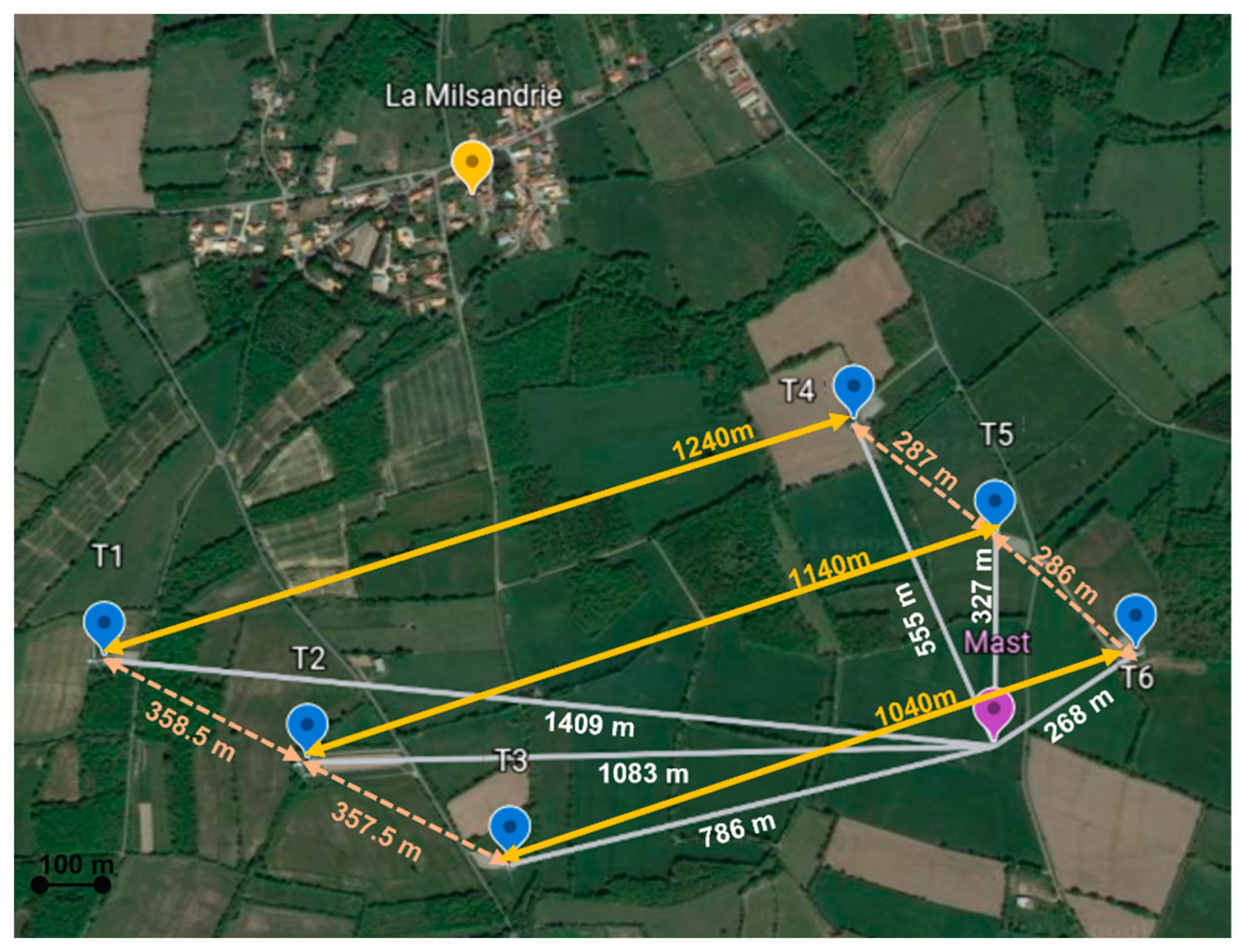
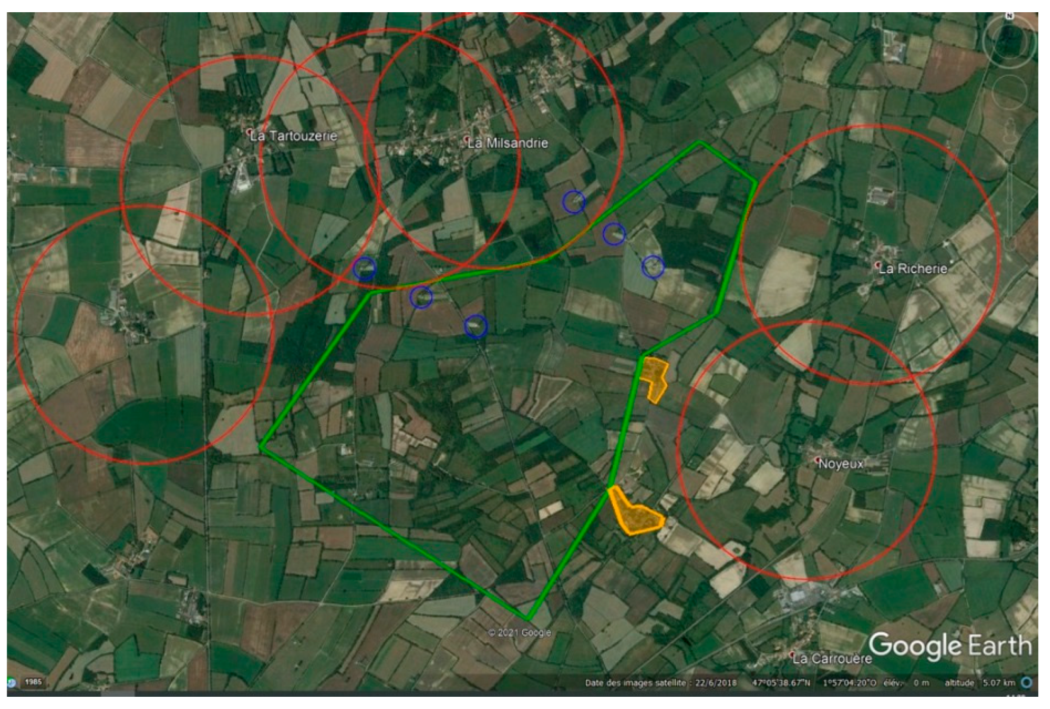
2.2.3. Wind Farm Site Description and Wind Turbine Characteristics

The wind farm used is situated in Saint-Hilaire-de-Chaléons, 30 km from Nantes city in France. Six Senvion MM92 wind turbines with rotor diameters of 92 m and hub heights of 78 m (Figure 2) are installed along two rows of three turbines each with a separation distance of 1.1 km, as shown in Figure 3. The distance between two neighboring turbines in the first row (T1, T2, and T3) is around 360 m, and it is around 287 m for the second row (T4, T5, and T6). The terrain is flat with an average altitude of 23 m above sea level and is mainly composed of pastures, meadows, and woods.

The wind farm site has also been equipped with a meteorological mast of 79 m, which is instrumented at four levels (10, 41, 53, and 79 m) with 3-D sonic anemometers, since October 2020. The data are collected at 20 Hz, which allowed us to compute at the various heights the mean wind speed and direction, the Reynolds stress tensor components, and the “sonic temperature” flux, which is a good proxy for the buoyancy flux.

2.2.4. Flight Operations with BOREAL

The BOREAL UAV was operated from 26 to 30 April 2021. The BOREAL company was in charge of the flight authorization requests and the operation of the UAV. The authorized flight zone was restricted to unpopulated areas near to the site, as delimited by the green line in Figure 4. Because of the presence of obstacles such as the wind turbines and the 79 m meteorological tower, the entire area north of T3 was not appropriate for flying. As a consequence, wind turbine wakes could not be sampled for undisturbed wind directions from ~90 to ~270 degrees (pink sector in Figure 3). In contrast, for wind coming from the [300–50°] sector (green sector in Figure 3), flights in the southern area of the authorized zone allowed us to document the wake of T3 (and possibly T2), and even the far-wake area of T6 for NE winds. The remaining wind directions (peach sector in Figure 3) were considered on the edge between favorable and unfavorable conditions. Moreover, air control authorities limited the flight height to 120 m above ground level (143 m above sea level), which approximately matched the top of the blade disk. Finally, the flights were authorized only when the wind speed was 5.5 m/s (20 km/h) at maximum, which was below the optimal operating conditions for the wind turbines. These severe flight restrictions imposed by air traffic control made the experiments difficult to achieve.

We chose to fly on racetracks that were staggered in relation to each other. The main orientation of the patterns was defined in order to be either aligned with or perpendicular to the mean wind direction or parallel to the T1-T2-T3 line. The latter allowed us to fly as close as possible to the wind turbines (Figure 5). Each of these patterns, called flight phases hereafter, lasted around 20 min and was performed two or three times during a flight. The flight altitudes were, in general, 90 m and 110 m above the ground level, which corresponded to one- and three-quarters of the turbine blade above the rotor, respectively. The axes closest to the wind turbine were performed at a distance of around 160 m, which corresponded to about twice the rotor diameter D.

We conducted five flights during the campaign, among which those performed on 28 and 30 April 2021 are presented in this paper. The corresponding flight patterns are presented in Figure 5. For the flight on 28 April, which lasted almost three hours, each flight phase was repeated three times against two times for the flight on 30 April that lasted two hours. All this information is summarized in

Table 1. Information about the date and trajectories of the two flights.

Flight Date and Time	Flight Altitudes	Orientation of Racetracks and Number of Repetitions of Flight Phases		Comments
28 April 2021 8:22 to 11:07 UTC	90 m and 110 m (agl)	Parallel to T1-to-T3 axis	3 times	During the first part of the flight, either both T2 and T3 turbines or only the T2 turbine were stopped.
		Almost south–north, east of T3	3 times
		Perpendicular to T1-to-T3 axis	3 times
30 April 2021 7:45 to 9:45 UTC	90 m and 110 m (agl)	Parallel to T1-to-T3 axis	2 times	All turbines were functioning.
		West–east	2 times
		Along the mean wind direction	2 times

.

3. Results and Discussion

3.1. Flight on 30 April 2021

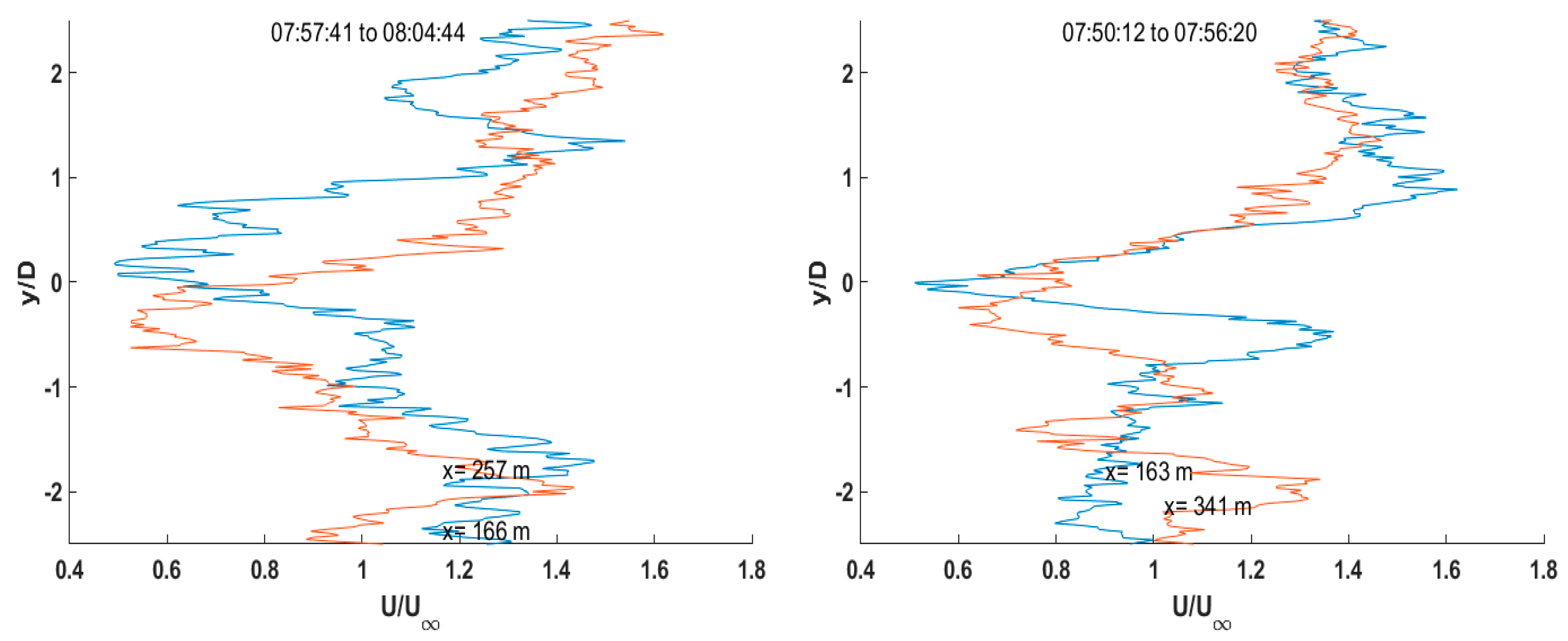
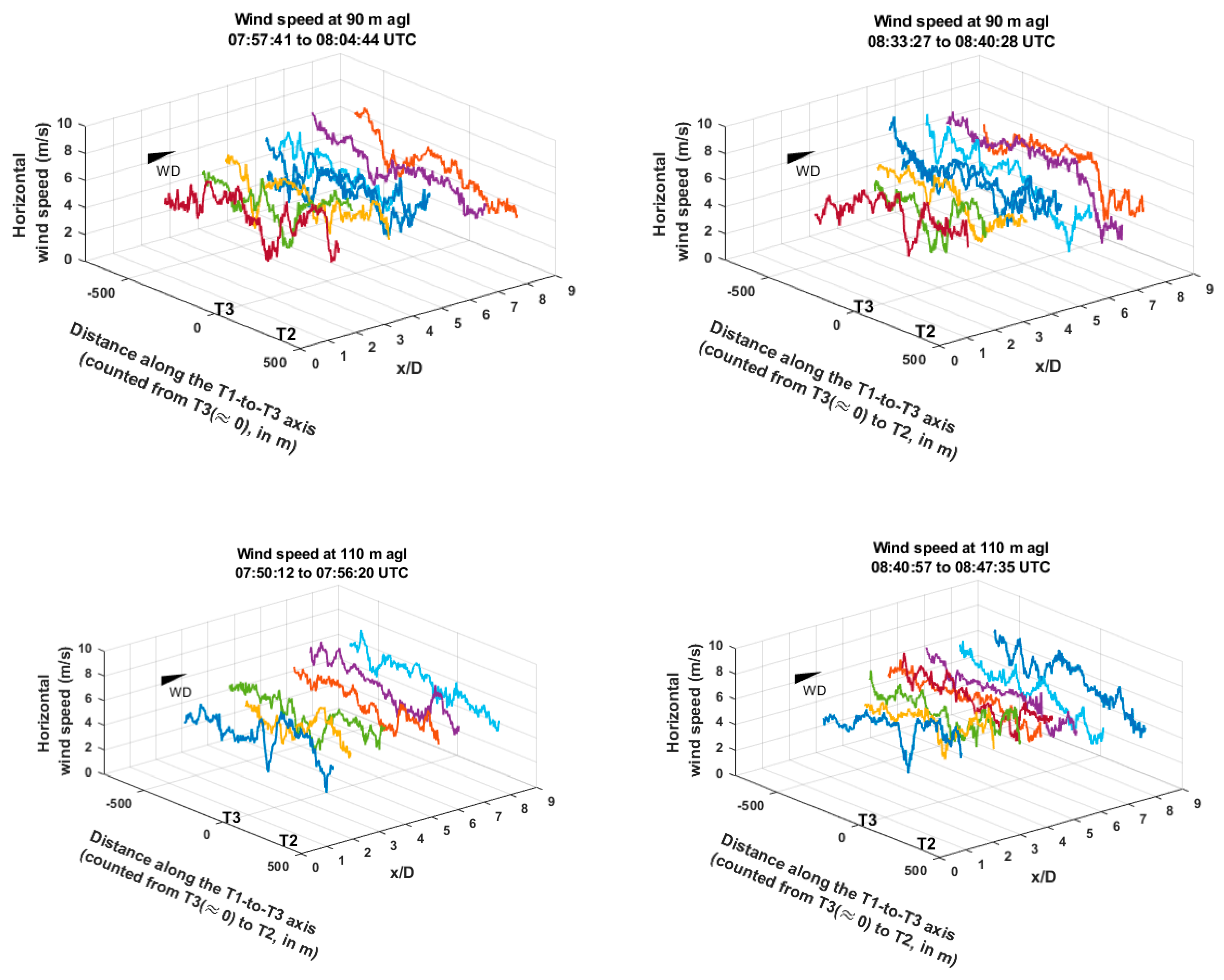
3.1.1. Instantaneous Wind Series

On 30 April, BOREAL performed four flight sequences with a racetrack orientation parallel to the axis linking T1 to T3. It flew at two average altitudes of around 90 and 110 m above ground level, which corresponded approximately to ¼ and ¾ of the turbine blade length above the hub height. As recalled in Table 1, all the turbines were in operation during the whole flight. Figure 6, represents the series of instantaneous horizontal wind speeds measured by the UAV in a frame constituted by the axes parallel (y-axis) and perpendicular (x-axis) to the T1-to-T3 line. The distance along the latter was normalized by the rotor diameter D. In such a representation, the mean wind (NNE in this case) approximately blew along the x axis, and the origin of the two horizontal axes was taken at the T3 wind turbine location. Only the straight part of the racetracks is represented here since the wind estimates were much less accurate during the turns. These straight runs of around 800 m on average were performed at distances from the T1-to-T3 line from 165 m to 800 m, corresponding from 1.8D to 8.7D. The observed wind series are a superposition of the wind variability related to turbulence and of the wake signature, itself containing an instantaneous variability. Extracting the continuous component of the wake would require numerous runs performed over the same track and averaging the wind series on these tracks, which was not the strategy chosen here. Nevertheless, in spite of the high variability of the wind series, we observe a large reduction in the wind speed behind T3 (i.e., at y ≈ 0) on all the runs performed at the closest distance from the turbines. The signal is clear on each of the four diagrams of Figure 5 and is a signature of the T3 wake. It is still observable on the second passage in distance from the turbines, except in the sequence performed at a 110 m agl between 07:50 and 07:56 UTC. As we moved on to runs away from the T1-to-T3 line, the wind deficit became less discernable from the other fluctuations in the series. At the easternmost part of the runs closest to the T1-to-T3 line, we were sometimes able to partially capture the wind reduction in the wake of the T2 turbine. It is discernible in the wind series shown in the left-hand side plots of Figure 5. Between the two weaker wind areas behind T2 and T3, there is a higher wind zone visible in the run performed at a 110 m agl close to the turbines. This could be the signature of the wind strengthening between the wind turbines observed in cumulative wakes behind several wind turbine rows since the wind direction placed the T2 and T3 turbines in the wake of T4 and T5, situated around 1 km upwind.

In Figure 7, we extracted from the series presented in Figure 6, at each of the two flight altitudes (90 m and 110 m agl) a pair of runs, the first being the closest to the T1-to-T3 axis (in blue) and the other at a farther distance behind (in orange). In these plots, the wind speed was normalized by the mean wind speed upstream of the turbines ${\mathrm{U}}_{\infty }$, and the position referred to the distance along the T1-to-T3 axis (0 being at T3) normalized by the rotor diameter D. The wind speeds were represented in the area comprised between y = −2.5 and y = +2.5D only. Such a representation allowed better detail of the wake structure close to the turbines. The plots clearly show that the wind deficit behind the turbine was similar both on the two axes and at the two heights, amounting to about 40% of the upstream value. This wind reduction area was not always centered behind the rotor, but could shift laterally for a fraction of the rotor diameter D. This displacement may be caused by horizontal meandering of the wake or by faster variations related to wake turbulence. Another common feature for the various series was that, at large negative y/D values, i.e., beyond T3 along the T1-to-T3 direction, the measured wind returned to values close to those observed upstream from the turbines, whereas for y/D values of 1 to 2, i.e., in the area downwind of the inter-T2–T3 zone, the wind speed exceeded by 40–50% the upstream values.

This is observed on each of the runs, whatever its height or distance from the turbines. The consistency between the various runs presented here would tend to confirm our previously invoked hypothesis of a cumulative wake behind the two wind turbine lines. Such bands of faster winds were nicely observed by Hirth et al., (2014) with a pair of scanning Doppler radars [5].

We wondered whether the signature of the tip vortices detached from the blade extremities in the wake area could be identified in the observed wind series. In Figure 7, the wind series at a 110 m agl performed at a distance of ~160 m from the T1-to-T3 line showed two higher wind zones at y/D = +1 and y/D = −0.5, i.e., on each side of the reduced wind in the core of the wake. However, it is difficult to be affirmative on the relation of these variations to tip vortices since the wind variations did not exceed the level of fluctuation in the turbulent wind series. Mauz et al., (2019) successfully made such observations of tip vortices with the MASC-3 UAV. However, they were able to fly at distances as close as 0.25D to the turbines for average wind conditions of 8 m/s. They obtained clear signatures with measured instantaneous wind bursts as high as 5–10 m/s when crossing the tip vortices, which were much higher than the values we measured [34]. Unfortunately, we certainly were at a distance that was too far from the rotor (around 2D) to be able to document tip vortices.

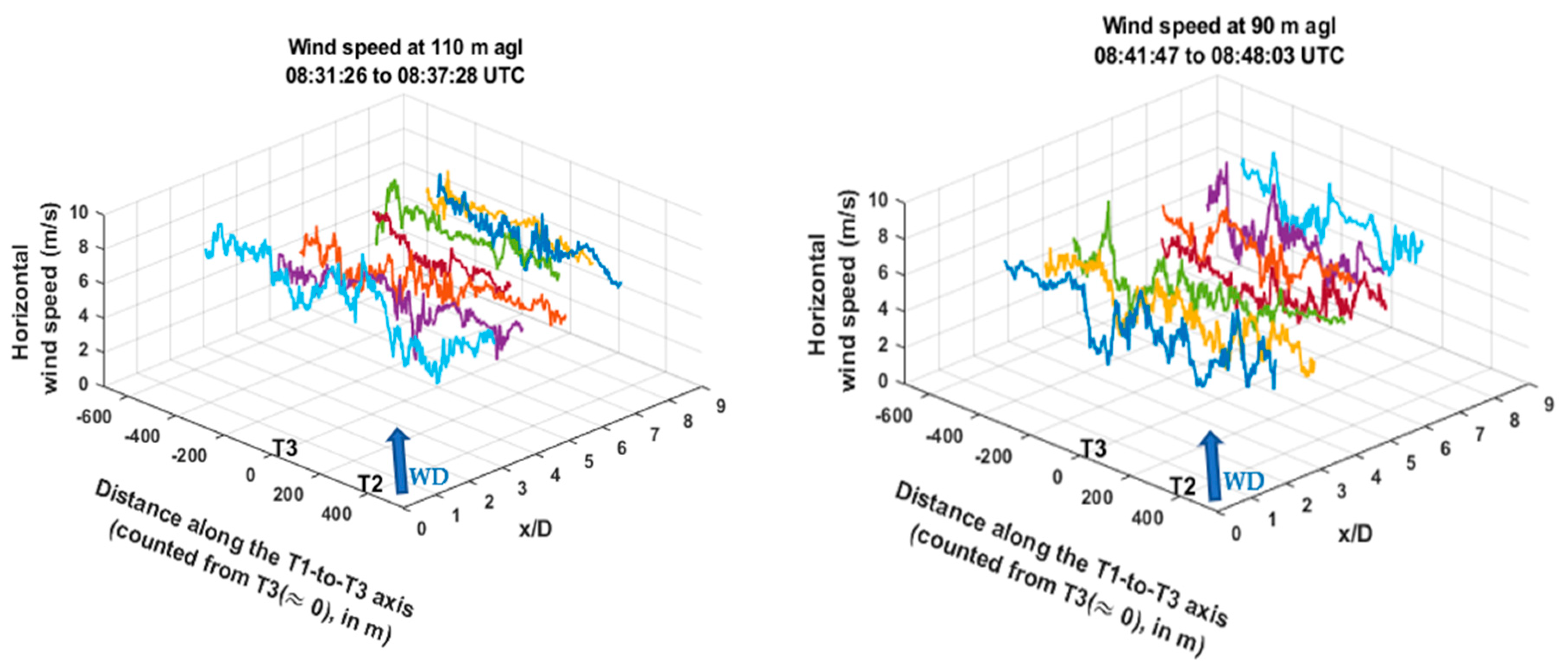
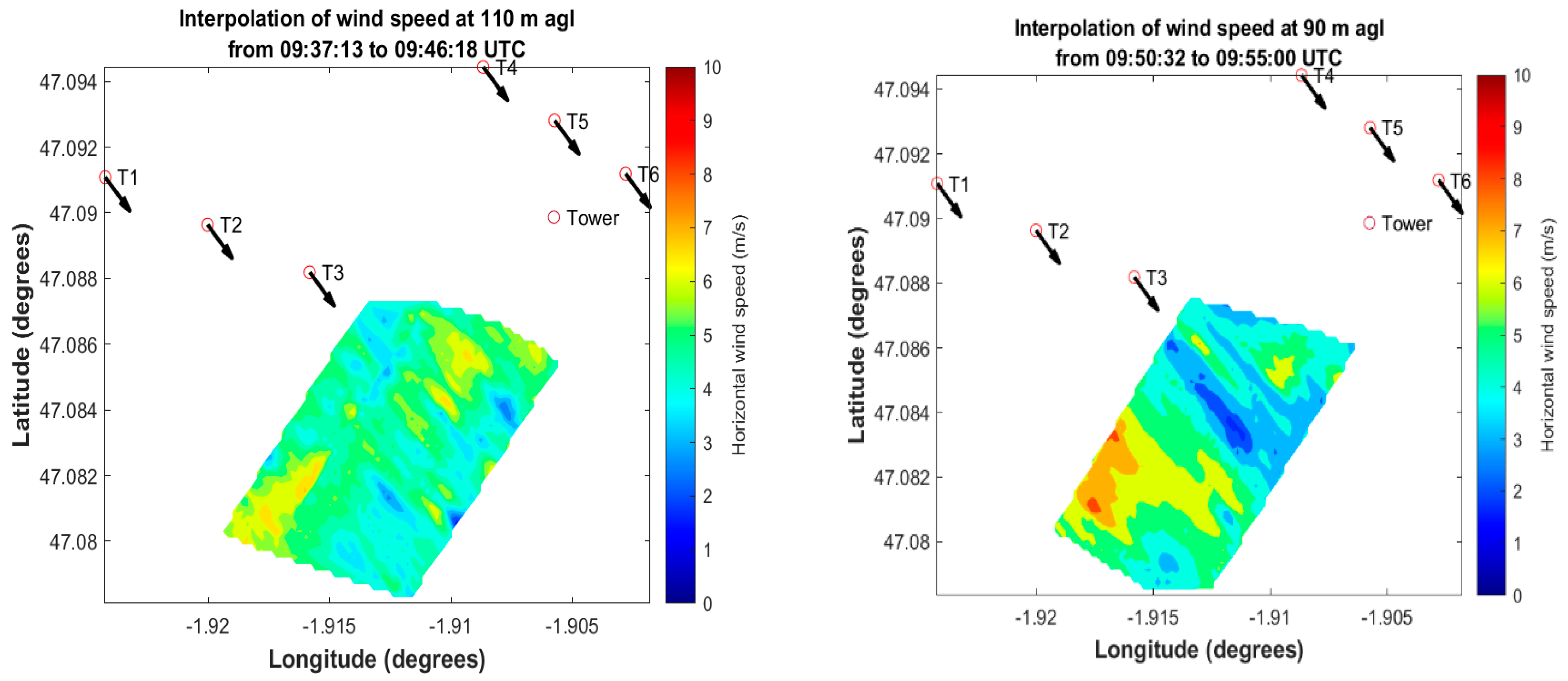
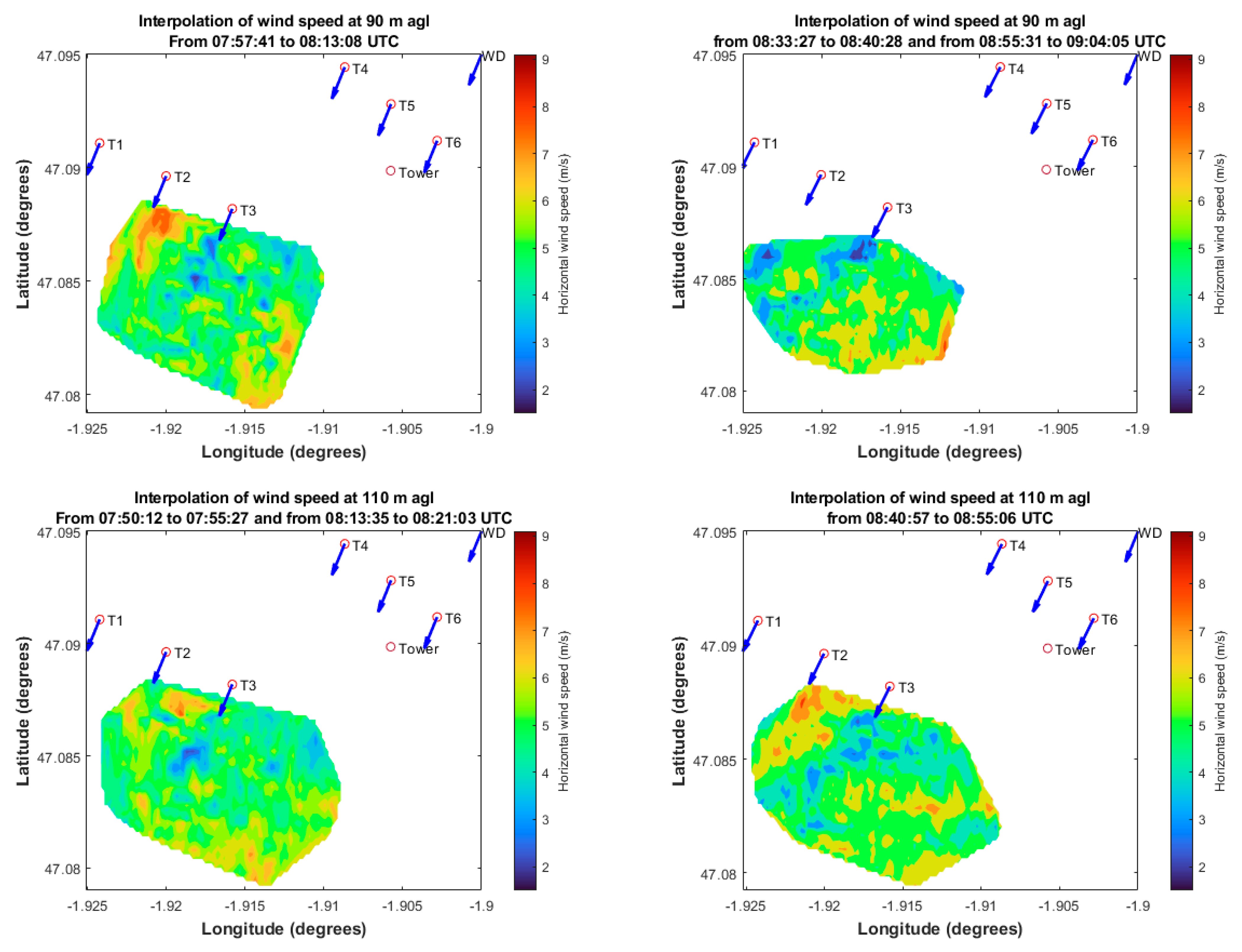
3.1.2. Horizontal Fields

The straight and level flight sequences performed at the same height during a quite short period of time (typically 15–20 min) were gathered together and spatially interpolated to build 2-D fields. In such a period of time, we could assume that the large-scale wind conditions do not vary much. This operation allowed us to combine flight runs with different headings in a single plot. Such interpolated wind fields are presented in Figure 8.

In spite of variability in wind speed related to instantaneous sampling of a turbulent field, some general features can be highlighted:

• The wind reduction in the wake area of T3 is observable for each of the two periods and at each of the two altitudes.
• This wind reduction is discernable behind the turbine down to about 400–500 m (~5D).
• The wake of T2 is on the edge on the interpolated fields and, thus, only appeared on the upper right field in the figure, thanks to the westernmost extension of three flight sequences during this flight phase.
• The wind strengthening behind the turbines line in the area between the T2 and T3 wakes is clear on all the plots except the upper right one. In this case, the area just behind T2 was not as well-covered as on the other plots, which explains the less discernable wind increase.
• Both the wind reduction behind the turbine and the wind increase between the turbine individual wakes seems to be more intense at 90 m (i.e., at a level just above the hub height) than at 110 m (just below the top of the blade disk). Porté-Agel et al., (2019) reported in their review paper that the maximum wind reduction was observed at the rotor level [2].

3.2. Flight on 28 April 2021

3.2.1. Instantaneous Wind Series

On 28 April, each flight phase was performed three times. The flight heights were identical to those of 30 April (90 and 110 m agl). We performed a series of racetracks parallel to the T1-to-T3 line, but since the wind was blowing from the NW, we performed a series that was crosswind-oriented for the area downwind of T3 (Figure 5). According to the wind configuration of this day and due to the delimited flight zone, only the wakes of the T2 and T3 turbines could be sampled.

As mentioned in Table 1, not all the turbines were operational during the whole flight, since during the first flight phase for a period of time (from 8:31 to 8:37 UTC), both the T2 and T3 turbines were out of service. The T3 turbine restarted at 8:41 UTC, and so did the T2 turbine at 8:50 UTC. During this period of time, BOREAL flew in parallel to the T1-to-T3 line. Figure 9 represents the instantaneous horizontal wind speed measured by BOREAL in a frame constituted by the axes parallel (y-axis) and perpendicular (x-axis) to the T1-to-T3 line, with the distance along the latter normalized by the rotor diameter D. Only the straight and level runs were represented, as for the previous flight. These runs had an 800 m length in average and were performed at distances from the T1-to-T3 line from 170 m to 800 m, corresponding from 1.85D to 8.7D. Notably, the wind was not aligned with the x-axis as it was for the preceding flight, and the flight axes were not perpendicular to the wake mean direction. The right plot represents the series measured at 110 m (agl) when both the T2 and T3 turbines were momentarily stopped, and the left plot represents the series measured at 90 m (agl) when only the T2 turbine was still out of service. The wind series on the left side of Figure 9 does not show a sudden reduction in the wind speed behind the T2 and T3 turbines since they were not operational, except for the nearest run (in sky-blue at 1.85D), where we observed this reduction, which could be explained by a short restart of the T2 turbine. However, when T3 restarted (right plot on Figure 9) we clearly observed a reduction in the wind speed behind both T2 and T3 on the closest runs from the T1-to-T3 line. Note that “behind” here means along the wind direction (see the arrow on the plot). This is the signature of the turbine wakes, which weakens when the runs are furthest from the T1-to-T3 line.

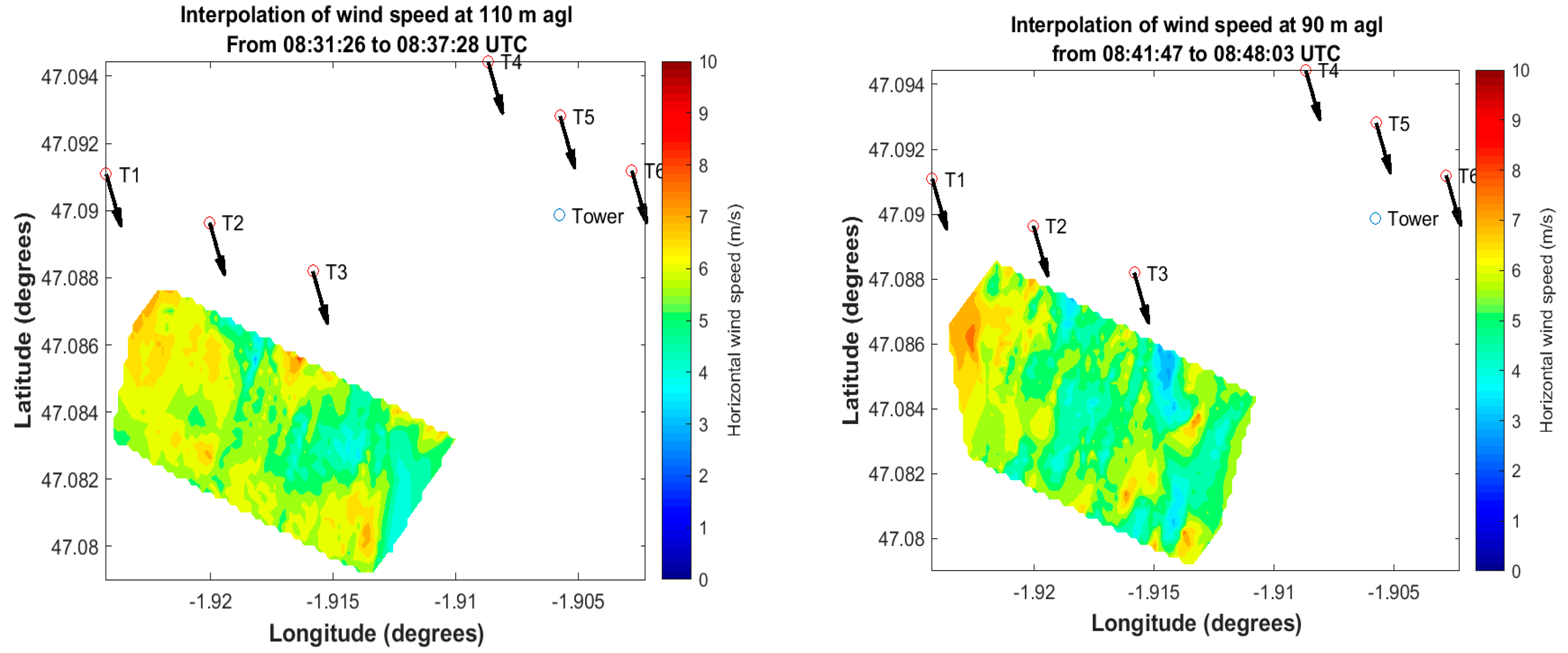
3.2.2. Horizontal Fields

The 2-D fields were built by spatial interpolation from the data collected on straight and level flight sequences for each specific flight phase. These phases lasted less than 10 min each; thus, we could assume that the large-scale wind conditions did not vary. BOREAL either flew in parallel to the T1-to-T3 line (Figure 10) or in a crosswind orientation (Figure 11). Figure 10 shows the 2-D fields corresponding to the data presented in Figure 9. When there were interruptions in the operation of the turbines. In contrast, Figure 11 represents two 2D fields at 110 m and 90 m (agl) when all the turbines were operating and the wind direction was slightly backing with respect to the previous flight phase. In Figure 10, only the wake of T3 was visible at 90 m (once the turbine has been restarted), with a weak intensity and downwind elongation. In Figure 11, with all the turbines in function there was a clear signature of the wind deficit in the wake of T3 at 90 m (i.e., the hub height), which extended downwind throughout the domain sampled by the UAV. At 110 m, however, the wind deficit was not as well-marked, and the wake was less intense. On the other hand, we observed at this level a series of bands aligned with the mean wind, with an alternance of higher and lower wind speeds. These bands were no longer observed in the southernmost part of the sampled domain, i.e., they were restricted to the wake area.

4. Conclusions

We presented the observations collected during two flights in the wake area of wind turbines. Thanks to the instrumentation installed onboard the BOREAL UAV, we were able to characterize the wind deficit in the area behind the turbines. A flight strategy based on horizontal racetracks performed at two heights (90 and 110 m agl) allowed us to examine the wake signature on individual runs, as well as to integrate a series of runs to build interpolated horizontal fields of the wind speed in the wake area. Such flight patterns, corresponding to the exploration of a horizontal plane at a given height, were short enough (~10 min) to consider the meteorological conditions at a large scale as not varying. Nevertheless, the individual runs were only able to capture an instantaneous signature on the wake, i.e., the superposition of its main characteristics and turbulent fluctuations. Though the wind deficit was clearly highlighted on the horizontal fields, it was difficult to accurately determine its horizontal extension (in both the lateral and longitudinal directions).

For the case of 30 April, the wind orientation allowed us to adequately sample the wake area with crosswind runs parallel to the wind turbine line (T1-to-T3 line). This allowed us to detect an overspeed zone between the wakes of two turbines. Such phenomena are observed in wind farms when the wind orientation ensures an overlapping of several wakes from upwind turbines. It is interesting to note that it was clearly detected in spite of the moderate wind speed (5–6 m/s on average) and the quite long distance between the two rows of turbines (~1 km). Hirth et al., (2015) observed well-organized overspeed bands, but for average windspeeds around two times higher than ours.

We demonstrated in this study the potential of BOREAL UAV to collect in situ observation of the wakes in wind farms. In particular, we validated the relevance of our flight strategy adopted for wake exploration since we were able to characterize the wind deficit downstream from the wind turbines as well as the wind strengthening between them. Nevertheless, the results presented here should be considered a first step toward a more comprehensive description of wakes. We were indeed faced with several limitations, from one side in relation with air traffic control restrictions (limited authorized flight zone, maximum wind speed for flight operations, maximum flight altitude, etc.) and on the other side linked to our flight strategy and limitations (flight runs too far from the turbines to document the near-wake area, single runs at a given place preventing statistical building of wind series, etc.).

We will be able to work in better conditions during forthcoming campaigns. Negotiations with air traffic control authorities resulted in a flight authorization for wind speeds up to 8.3 m/s and a higher maximum altitude, which will allow us to document the wakes in their complete vertical extension, as well as to make observations in wind speed conditions corresponding to the optimal operating mode of the turbines. We will take advantage of having a heavy, robust platform able to fly even in adverse, highly turbulent conditions. In our future campaigns, we will also adapt our flight strategy to sample the wake as close as possible to the wind turbine line, to repeat the same run several times to be able to extract structural characteristics, such as the accurate extension of the wakes and the detection of eddies at the extremity of the blades (tip vortices), and to obtain more quantitative data on the wind deficit and overspeed bands. Thanks to the UAV capability to observe wind fluctuations with a spatial resolution of around 3 m, we should also be able to observe the turbulence characteristics of the wakes.

A major objective of the MOMENTA project is to bring more insights and better understanding of WIT in order to improve the design and layout of wind farms. Simulations of the interactions between wind turbines, the surface, and the ABL should be performed in atmospheric LESs in a way similar to what was conducted for the Horns Rev 1 wind farm. In the future, such tools will help to optimize the layout of the wind farms in terms of reducing loads and enhancing the energy produced [36].

References

1. GWEC-Global-Wind-Report-2021. Available online: https://gwec.net/wp-content/uploads/2021/03/GWEC-Global-Wind-Report-2021.pdf (accessed on 17 March 2022).
2. Porté-Agel, F.; Bastankhah, M.; Shamsoddin, S. Wind-Turbine and Wind-Farm Flows: A Review. Bound. Layer Meteorol. 2020, 174, 1–59. [Google Scholar] [CrossRef] [PubMed] [Green Version]
3. Lissaman, P.B.S.; Zambrano, T.G.; Gyatt, G.W. Wake Structure Measurements at the Mod-2 Cluster Test Facility at Goodnoe Hills; PNL-4572; Pacific Northwest Laboratory: Washington, DC, USA, 1983; p. 6463031. [Google Scholar]
4. Kumer, V.-M.; Reuder, J.; Svardal, B.; Sætre, C.; Eecen, P. Characterisation of Single Wind Turbine Wakes with Static and Scanning WINTWEX-W LiDAR Data. Energy Procedia 2015, 80, 245–254. [Google Scholar] [CrossRef] [Green Version]
5. Hirth, B.D.; Schroeder, J.L.; Gunter, W.S.; Guynes, J.G. Coupling Doppler Radar-Derived Wind Maps with Operational Turbine Data to Document Wind Farm Complex Flows. Wind Energy 2015, 18, 529–540. [Google Scholar] [CrossRef]
6. Stevens, R.; Gayme, D.; Meneveau, C. Coupled Wake Boundary Layer Model of Wind-Farms. J. Renew. Sustain. Energy 2014, 7, 023115. [Google Scholar] [CrossRef] [Green Version]
7. Stevens, R.J.A.M.; Gayme, D.; Meneveau, C. Using the Coupled Wake Boundary Layer Model to Evaluate the Effect of Turbulence Intensity on Wind Farm Performance. J. Phys. Conf. Ser. 2015, 625, 012004. [Google Scholar] [CrossRef] [Green Version]
8. Jensen, N.O. A Note on Wind Generator Interaction; Y RISØ-M-2411; Risø National Laboratory: Roskilde, Denmark, 1983. [Google Scholar]
9. Neunaber, I.; Obligado, M.; Peinke, J.; Aubrun, S. Application of the Townsend-George Wake Theory to Field Measurements of Wind Turbine Wakes. J. Phys. Conf. Ser. 2021, 1934, 012004. [Google Scholar] [CrossRef]
10. Maalouf, C.; Dobrev, I.; Massouh, F. Exploration Des Structures Tourbillonnaires Dans Le Sillage d’un Rotor Éolien. In Proceedings of the CFSER 2010 1ère Conférence Franco-Syrienne sur les énergies Renouvelables, Damascus, Syria, 24–28 October 2010. [Google Scholar]
11. Yang, Z.; Sarkar, P.; Hu, H. Visualization of the Tip Vortices in a Wind Turbine Wake. J. Vis. 2012, 15, 39–44. [Google Scholar] [CrossRef]
12. Odemark, Y. Wakes behind Wind Turbines—Studies on Tip Vortex Evolution and Stability. 2012. Available online: https://www.diva-portal.org/smash/get/diva2:524104/FULLTEXT01.pdf (accessed on 17 March 2022).
13. Käsler, Y.; Rahm, S.; Simmet, R.; Kühn, M. Wake Measurements of a Multi-MW Wind Turbine with Coherent Long-Range Pulsed Doppler Wind Lidar. J. Atmos. Ocean. Technol. 2010, 27, 1529–1532. [Google Scholar] [CrossRef] [Green Version]
14. Aitken, M.L.; Banta, R.M.; Pichugina, Y.L.; Lundquist, J.K. Quantifying Wind Turbine Wake Characteristics from Scanning Remote Sensor Data. J. Atmos. Ocean. Technol. 2014, 31, 765–787. [Google Scholar] [CrossRef]
15. Wildmann, N.; Hofsäß, M.; Weimer, F.; Joos, A.; Bange, J. MASC—A Small Remotely Piloted Aircraft (RPA) for Wind Energy Research. Adv. Sci. Res. 2014, 11, 55–61. [Google Scholar] [CrossRef] [Green Version]
16. Reuder, J.; Båserud, L.; Kral, S.; Kumer, V.; Wagenaar, J.W.; Knauer, A. Proof of Concept for Wind Turbine Wake Investigations with the RPAS SUMO. Energy Procedia 2016, 94, 452–461. [Google Scholar] [CrossRef] [Green Version]
17. Medici, D.; Ivanell, S.; Dahlberg, J.-Å.; Alfredsson, P.H. The Upstream Flow of a Wind Turbine: Blockage Effect. Wind Energy 2011, 14, 691–697. [Google Scholar] [CrossRef]
18. Ivanell, S.; Mikkelsen, R.; Sørensen, J.N.; Henningson, D. Stability Analysis of the Tip Vortices of a Wind Turbine. Wind Energy 2010, 13, 705–715. [Google Scholar] [CrossRef]
19. Premaratne, P.; Hu, H. A Novel Vortex Method to Investigate Wind Turbine Near-Wake Characteristics. In 35th AIAA Applied Aerodynamics Conference; American Institute of Aeronautics and Astronautics: Denver, CO, USA, 2017. [Google Scholar]
20. Sherry, M.; Nemes, A.; Lo Jacono, D.; Blackburn, H.M.; Sheridan, J. The Interaction of Helical Tip and Root Vortices in a Wind Turbine Wake. Phys. Fluids 2013, 25, 117102. [Google Scholar] [CrossRef] [Green Version]
21. Yang, X.; Hong, J.; Barone, M.; Sotiropoulos, F. Coherent Dynamics in the Rotor Tip Shear Layer of Utility-Scale Wind Turbines. J. Fluid Mech. 2016, 804, 90–115. [Google Scholar] [CrossRef] [Green Version]
22. Felli, M.; Camussi, R.; Felice, F.D. Mechanisms of Evolution of the Propeller Wake in the Transition and Far Fields. J. Fluid Mech. 2011, 682, 5–53. [Google Scholar] [CrossRef] [Green Version]
23. Ashton, R.; Viola, F.; Camarri, S.; Gallaire, F.; Iungo, G.V. Hub Vortex Instability within Wind Turbine Wakes: Effects of Wind Turbulence, Loading Conditions, and Blade Aerodynamics. Phys. Rev. Fluids 2016, 1, 073603. [Google Scholar] [CrossRef]
24. Coudou, N.; Buckingham, S.; Bricteux, L.; van Beeck, J. Experimental Study on the Wake Meandering Within a Scale Model Wind Farm Subject to a Wind-Tunnel Flow Simulating an Atmospheric Boundary Layer. Bound. Layer Meteorol. 2018, 167, 77–98. [Google Scholar] [CrossRef]
25. Howard, K.B.; Singh, A.; Sotiropoulos, F.; Guala, M. On the Statistics of Wind Turbine Wake Meandering: An Experimental Investigation. Phys. Fluids 2015, 27, 075103. [Google Scholar] [CrossRef]
26. Carbajo Fuertes, F.; Markfort, C.D.; Porté-Agel, F. Wind Turbine Wake Characterization with Nacelle-Mounted Wind Lidars for Analytical Wake Model Validation. Remote Sens. 2018, 10, 668. [Google Scholar] [CrossRef] [Green Version]
27. McKay, P.; Carriveau, R.; Ting, D.S.-K. Wake Impacts on Downstream Wind Turbine Performance and Yaw Alignment. Wind Energy 2013, 16, 221–234. [Google Scholar] [CrossRef]
28. Marathe, N.; Swift, A.; Hirth, B.; Walker, R.; Schroeder, J. Characterizing Power Performance and Wake of a Wind Turbine under Yaw and Blade Pitch. Wind Energy 2016, 19, 963–978. [Google Scholar] [CrossRef]
29. Kocer, G.; Mansour, M.; Chokani, N.; Abhari, R.S.; Müller, M. Full-Scale Wind Turbine Near-Wake Measurements Using an Instrumented Uninhabited Aerial Vehicle. J. Sol. Energy Eng. 2011, 133, 041011. [Google Scholar] [CrossRef]
30. Kocer, G.; Chokani, N.; Abhari, R.S. Detailed Measurements in the Wake of a 2MW Wind Turbine. In European Wind Energy Conference and Exhibition 2012, EWEC 2012, Copenhagen, Denmark, 16–19 April 2012; European Wind Energy Association: Brussels, Belgium, 2012; Volume 1, pp. 448–454. [Google Scholar]
31. Mansour, M.; Kocer, G.; Lenherr, C.; Chokani, N.; Abhari, R.S. Seven-Sensor Fast-Response Probe for Full-Scale Wind Turbine Flowfield Measurements. J. Eng. Gas Turbines Power 2011, 133, 081601. [Google Scholar] [CrossRef]
32. Rautenberg, A.; Allgeier, J.; Jung, S.; Bange, J. Calibration Procedure and Accuracy of Wind and Turbulence Measurements with Five-Hole Probes on Fixed-Wing Unmanned Aircraft in the Atmospheric Boundary Layer and Wind Turbine Wakes. Atmosphere 2019, 10, 124. [Google Scholar] [CrossRef] [Green Version]
33. Båserud, L.; Flügge, M.; Bhandari, A.; Reuder, J. Characterization of the SUMO Turbulence Measurement System for Wind Turbine Wake Assessment. Energy Procedia 2014, 53, 173–183. [Google Scholar] [CrossRef] [Green Version]
34. Mauz, M.; Rautenberg, A.; Platis, A.; Cormier, M.; Bange, J. First Identification and Quantification of Detached-Tip Vortices behind a Wind Energy Converter Using Fixed-Wing Unmanned Aircraft System. Wind Energy Sci. 2019, 4, 451–463. [Google Scholar] [CrossRef] [Green Version]
35. Alaoui-Sosse, S.; Durand, P.; Medina, P.; Pastor, P.; Gavart, M.; Pizziol, S. BOREAL- A Fixed-Wing Unmanned Aerial System for the Measurement of Wind and Turbulence in the Atmospheric Boundary Layer. J. Atmos. Ocean. Technol. 2022, 39, 387–402. [Google Scholar] [CrossRef]
36. Joulin, P.-A.; Mayol, M.L.; Masson, V.; Blondel, F.; Rodier, Q.; Cathelain, M.; Lac, C. The Actuator Line Method in the Meteorological LES Model Meso-NH to Analyze the Horns Rev 1 Wind Farm Photo Case. Front. Earth Sci. 2020, 7, 350. [Google Scholar] [CrossRef] [Green Version]
Figure 1. Schematic representation of the three wake regions and of the wake meandering phenomenon, which is indicated by the curved lines. The wind profiles upstream (in black) and downstream (in blue) from the turbine are shown.
Atmosphere 13 00775 g001
Figure 2. Schematic showing the wind turbine dimensions and the flight altitudes.
Atmosphere 13 00775 g002
Figure 3. Localization of the six wind turbines (T1, T2, T3, T4, T5, and T6) indicated by the blue marks. The instrumented mast is pointed out by the purple mark. The distances between the turbines are indicated by the yellow (dashed and full) arrows. The distances between each turbine and the mast are indicated by the grey lines. The geographical coordinates of the mast are 47.090° N, 1.906° W.
Atmosphere 13 00775 g003
Figure 4. The authorized flight area is delimited with the green line. The small blue circles are the wind turbines. The red circles border the populated zones. The three wind sectors (WSs) are shown in green, peach, and pink (see text for more details).
Atmosphere 13 00775 g004
Figure 5. The flight patterns on 28 April (left side) and on 30 April (right side). The positions of the six wind turbines and their designation names are pointed out by T1, T2, T3, T4, T5, and T6 in the figure. The localization of the 79 m instrumented mast is indicated by “Tower” in the figure. The blue arrows indicate the average wind direction (WD) for each flight. The “x” and “y” arrows mark the frame for the plots in the forthcoming figures.
Atmosphere 13 00775 g005
Figure 6. D representation of the instantaneous horizontal wind speed measured during the 30 April flight when BOREAL was flying parallel to the T1-to-T3 axis at distinct moments and different flight altitudes. The x-axis represents the distance between the UAV and the T1-to-T3 axis normalized by the rotor diameter D (=92 m). The black arrows indicate the wind direction (WD). The remaining axis represents the distance (in m) along the T1-to-T3 axis.
Atmosphere 13 00775 g006
Figure 7. Instantaneous wind speed normalized by the mean wind speed upstream of the turbines U vs. the distance along the T1-to-T3 axis normalized by rotor diameter D. Two series are represented on each graph. The blue corresponds to the run at the closest distance to the T1-to-T3 axis (x = 166 and 163 m) and the orange is farther out in the wake (x = 257 and 341 m). Left: runs at a 90 m agl. Right: runs at a 110 m agl.
Atmosphere 13 00775 g007
Figure 8. 2-D fields of horizontal wind speed measured on 30 April at distinct moments at 90 m (top) or 110 m agl (bottom). The blue arrows represent the direction of the wind averaged over the interpolated field during the corresponding sequence. T1 to T6 are the localizations of the six wind turbines.
Atmosphere 13 00775 g008
Figure 9. 3-D representation of the instantaneous horizontal wind speed measured during the flight on 28 April when BOREAL flew parallel to the T1-to-T3 axis at distinct moments and different flight altitudes. X represents the distance between the UAV and the T1-to-T3 axis normalized by the rotor diameter D (=92 m). The blue arrows indicate the average wind direction (WD). The remaining axis represents the distance (in m) to the horizontal axis perpendicular to x passing through T3.
Atmosphere 13 00775 g009
Figure 10. 2-D fields of the horizontal wind speed measured on 28 April at different moments. Left plot: at 110 m (agl) when T2 and T3 were not functioning. Right plot: at 90 m (agl) after the T3 turbine restarted. The black arrows represent the wind direction average during the flight phase.
Atmosphere 13 00775 g010
Figure 11. 2-D fields of the horizontal wind speed measured on 28 April when all the wind turbines were operating. Left plot: at 110 m (agl). Right plot: at 90 m (agl). The black arrows represent the wind direction average during this specific flight phase. T1 to T6 are the localizations of the six wind turbines.
Atmosphere 13 00775 g011