Urban Climate Risk Mitigation via Optimal Spatial Resource Allocation

Abstract

Decision makers (DMs) who are involved in urban planning are often required to allocate finite resources (say, money) to improve outdoor thermal comfort (OTC) levels in a region (e.g., city, canton, country). In this paper, for the first time, we address the following two questions, which are directly related to this requirement: (1) How can the statistical properties of the spatial risk profile of an urban area from an OTC perspective be quantified, no matter which OTC index the DM chooses to use? (2) Given the risk profile, how much and where should the DM allocate the finite resources to improve the OTC levels? We answer these fundamental questions by developing a new and rigorous mathematical framework as well as a new class of models for spatial risk models. Our approach is based on methods from machine learning: first, a surrogate model of the OTC index that provides both accuracy and mathematical tractability is developed via regression analysis. Next, we incorporate the imperfect climate model and derive the statistical properties of the OTC index. We present the concept of spatio-temporal aggregate risk (STAR) measures and derive their statistical properties. Finally, building on our derivations, we develop a new algorithm for spatial resource allocation, which is useful for DMs and is based on modern portfolio theory. We implemented the tool and used it to illustrate its operation on a practical case of the large-scale area of Singapore using a WRF climate model.

1. Introduction

An accurate assessment of the environmental risk of urban climate events is of great importance for populations, authorities, and decision makers (DMs) [1,2]. Spatial risk assessment provides DMs with the necessary information to make informed decisions and allocate resources in a meaningful way that aims at improving the overall welfare of the population. The allocation of resources is central to the DMs’ operation and may have long-term implications, and should, therefore, be accurately modeled [3,4,5].

While there are a myriad of aspects that DMs should take into account, one aspect which is widely accepted as important is the perception of thermal comfort experienced by the population [6,7]. The thermal comfort of the population affects multiple aspects of life and directly and indirectly contributes to the well-being of the population [8]. In particular, outdoor thermal comfort (OTC) is a key indicator of people’s well-being, productivity, and happiness in general [9,10,11]. Therefore, in this work, we concentrate on OTC as a key indicator of people’s well-being and acknowledge its contribution to key performance indicators of a city. To reflect this, a myriad of different indices have been developed; see [12] for an overview. The OTC indices can be divided into two main categories: rational or empirical indices. The rational indices are based on heat transfer and energy balance principles of a typical human body in relation to its physical environment [13]. The second type of indices is based on empirical studies of the subjective experience of OTC in relation to meteorological phenomena [9,10]. While rational indices are based on fundamentals of physics and bio-meteorology, thereby making them more favorable than their empirical counterparts, they may be more complicated and less intuitive to understand. They also lack mathematical tractability and can only be evaluated through numerical calculations; see, for example, the evaluation of physiological equivalent temperature (PET) in [14].

1.1. Literature Review on OTC-Informed Urban Planning

We begin by stating that, currently, there are no works that address the problem of resource allocation and aims at improving OTC levels at different spatial locations jointly. In our previous works, we have developed a framework to score and rank different urban designs, but the important aspect of (spatial) resource allocation was not addressed and the analysis concentrated on small-scale developments [15,16,17]. While our work is the first to address this problem, there have been some works on related topics that investigated the concept of improving OTC levels via different intervention strategies, and here we review some of them. The evaluation of the quality of urban spaces from an OTC perspective has been the focus of many previous works; see, for example [18,19,20,21,22]. In [23], the authors investigated the OTC perception of subjects and their physical wellbeing. In [24], the authors reviewed the effects of green spaces and plants on the micro-climate, urban heat islands, and human outdoor thermal comfort. In [20], the authors conducted detailed CFD simulations under a large range of wind conditions and evaluated the OTC under each scenario. In [21], the authors examined the effect of plant types, arrangements, and their orientation on OTC. More recently, in [25], the authors developed a method to optimize the OTC levels by setting the optimal parameters of building heights, street widths, and orientations. While those studies provide many important insights regarding the impact of different techniques and technologies on OTC improvements, an important gap still remains when considering the problem of improving OTC on a large geographical scale (i.e., a city or country). Those are still open questions which have been not been fully addressed. For example, in [26], the authors provide an overview on how machine learning-based methods could be used in order to help DMs make “geographically differentiated” allocations of resources in a systematic way. In [27], the authors developed a method to create climate zoning based on the relationship between spatial temperature distribution and the various associated factors using observed data and numerical simulations.

Those papers make progress in mapping geographical areas and their OTC quality. Still, an open question remains: How should DMs allocate their financial resources in order to improve OTC on a large geographical scale? It could be that some regions experience worse OTC levels than others. Should such regions receive more resources in order to improve their OTC levels? Or, perhaps, would the finite resources be better used if allocated to regions where the OTC levels are mediocre, aiming, thus, at improving those areas while neglecting the regions with low- and high-quality OTC levels?

Similar to [26,27], we are also interested in the concept of “geographically differentiated” allocations of resources. We, however, develop a novel systematic approach for addressing this problem using the notions of risk modeling and resource allocation methods.

1.2. The Proposed Framework—Spatial Resource Allocation for OTC Enhancement

Ultimately, the DM (say, a government agency) is required to allocate finite financial resources in order to improve OTC levels in a geographical area. A common approach for allocating the resources would be to partition the physical domain into a finite number of regions, and allocate the money to each region according to some decision mechanism. The problem of spatial resource allocation is common in many areas of engineering, including wireless communication [28,29], logistics and planning [30], transportation networks [31,32], and many others. Much less attention has been given to spatial resource allocation in the context of urban-climate management. To address this open question, we develop a spatial risk model and link it to a spatial resource allocation method, which is based on similar concepts to the ones used in modern portfolio allocation (MPA), known as the Markowitz mean-variance model [33,34]. In order to be able to develop such a tractable mathematical framework for resource allocation, we need to be able to express the OTC equations in closed form. This can be obtained by using a machine learning technique known as surrogate models. Surrogate models refers to a model of a model; that is, instead of using the original model, we replace it with a simpler and mathematically tractable one. This way, we can gain the desired mathematical tractability at the expense of possible loss of accuracy. The loss of accuracy can be easily calculated (via model validation techniques) and then can be incorporated into the model, thus retaining all statistical information available. One more important aspect which is usually overlooked or ignored is the simple fact that no model is perfect [35]. Even the most advanced state-of-the-art climate models are still simplifications of reality and incur estimation errors [36]. Validating the model is paramount in order to quantify the magnitude and statistical properties of the estimation error of the various climate variables [37]. Then, incorporating the errors from both sources (that is, the surrogate and climate models) is required, if one wishes to accurately quantify the OTC spatial risk. Other works which have taken climate and climate model uncertainty into consideration in urban design decision making include [15,16,37]. However, these works did not consider the use of a surrogate model and only considered climate model uncertainty.

A graphical illustration of the framework that contains the aforementioned components is depicted in Figure 1.

1.3. Goals of This Paper

The goals of this paper are threefold:

• Develop a generic and accurate regression-based surrogate model that is suitable for a wide range of OTC index models;
• Introduce and develop the notions of spatial risk measures in the context of urban climate and provide a unified framework for spatial risk profile estimation;
• Develop a spatial (geographically differentiated) resource allocation scheme to improve the overall OTC levels in a region of interest.

We summarize the main contributions that we make in this paper:

C1.

We develop a surrogate model for any OTC index that is based on multiple non-linear regressions with interactions (Section 2);

C2.

We derive the statistical properties of the OTC index under both climate and surrogate model uncertainty (Section 3);

C3.

We present two risk measures and derive their properties for the OTC index (Section 4);

C4.

We show how to spatially aggregate the risk in order to obtain the risk of a spatial domain (Section 4);

C5.

We develop a new algorithm for spatial resource allocation that is based on the aggregate risk model (Section 5).

1.4. Mathematical Notations

We now introduce much of the notations we will use in the rest of the paper and recall certain important notions. The symbols $\mathbb{R}$ and $\mathcal{C}$ denote the real and integer numbers, respectively. Random variables are denoted by upper case letters and their realizations by lower case letters. In addition, bold will be used to denote a vector or matrix quantity, and lower subscripts refer to the element of a vector or matrix. We denote the distribution of random variable X by $X\sim p_X\left(x\right)$. The operator $\mathbb{E}\left[x\right]:=\int xp\left(x\right)\mathrm{d}x$ is the statistical mean of the random variable X, and the operator $\mathbb{V}\mathrm{ar}\left[X\right]:=\mathbb{E}\left[{\left(X-\mathbb{E}\left[X\right]\right)}^2\right]$ is the statistical variance of the random variable X. The notation $\mathbf{x}\sim \mathcal{N}\left(\mu ,{\sigma }^2\right)$ denotes a normally distributed R.V. with the mean and variance given by $\mu$ and ${\sigma }^2$, respectively. The notation $\mathbf{x}\sim \mathcal{MVN}\left(\mu ,\mathsf{\Sigma }\right)$ denotes a multivariate normally distributed R.V., with the mean vector and covariance matrix given by $\mu$ and $\mathsf{\Sigma }$, respectively. The notation $z\sim {\chi }^2\left(k,\lambda \right)$ denotes the non-central chi-squared distribution with degrees of freedom k and non-centrality parameter $\lambda$. The symbols used throughout the paper are presented in

Table 1. Table of Notations.

Variable	Meaning
$\mathcal{Z}$	Physical region of interest.
$\mathcal{T}$	Time duration, with $t\in \mathcal{T}$ as the time stamp.
$x_i\left(\mathbf{z},t\right)$	The i-th climatic variable at location $\mathbf{z}$ and time t.
${\mathbf{x}}_s\left(\mathbf{z},t\right)$	Vector of the climatic variables at location $\mathbf{z}$ and time t.
$y\left(\mathbf{z},t\right)$	Spatio-temporal OTC index process.
${\widehat{x}}_i\left(\mathbf{z},t\right)$	Estimated value of the i-th climatic variable.
${\widehat{\mathbf{x}}}_s\left(\mathbf{z},t\right)$	Estimated vector of climatic variables.
$\zeta \left(\mathbf{x},t\right)$	Climate model estimation error.
$\rho \left(y\right)$	Risk measure.
$\mathbb{T}\left(\mathit{y}\right)$	Aggregation function.
$\Lambda \left(\overline{y},\alpha \right)$	Utility function
$\Delta \left(\overline{y},\alpha \right)$	Marginal OTC intervention impact.
$\overline{\rho }\left(\mathit{y}\left(\mathbf{z}\in {\mathcal{Z}}_a,t\in {\mathcal{T}}_a\right)\right)$	Spatio-temporal aggregate risk (STAR) measure.

.

2. Generic Representation of OTC Indices via a Surrogate Model

As mentioned before, there are hundreds of OTC indices and it would be impossible to analyze each one separately. Instead, we are interested in a single modeling approach which can encompass as many indices as possible, making our approach general. In order to achieve that we develop a generic representation of any OTC model via a statistical regression model, known as surrogate model. Having a single family of regression models will simplify the analysis, allow for interpretability, and provide mathematical tractability. Any OTC index can be expressed as a mapping from an input space (usually high-dimensional) to an output space (one-dimensional). More specifically, as it is commonly used in machine learning, we treat the OTC model as a black box which contains a set of n input climatic variables, $\mathbf{x}\in {\mathbb{R}}^n$, and other non-climatic variables (e.g., personal parameters), $\xi \in \Xi$, and a single output variable, $y\in \mathbb{R}$. The OTC index model can be understood as a mapping from the input space to the output space $g\left(\mathbf{x},\xi \right):{\mathbb{R}}^n\times \Xi ⟼\mathbb{R}$. We now provide a formal definition of the OTC index model.

Definition 1

(Generic OTC index model). Let $\mathbf{x}:=\left[x_1,\dots ,x_n\right]\in {\mathbb{R}}^n$ denote the climatic variables, and let $\xi :=\left[{\xi }_1,\dots ,{\xi }_m\right]\in \Xi$ denote non-climatic variables. Let $y\in \mathbb{R}$ be the OTC index value; then, a generic OTC index model can be expressed as:

$$\begin{array}{c}\hfill y=g\left(\underset{\mathbf{x}}{\underbrace{x_1,\dots ,x_n}},\underset{\xi }{\underbrace{{\xi }_1,\dots ,{\xi }_m}}\right),\end{array}$$

where $g\left(\mathbf{x},\xi \right):{\mathbb{R}}^n\times \Xi ⟼\mathbb{R}$ is the mathematical representation of the OTC index model.

We now provide two examples which illustrate how this definition applies for two widely used OTC indices, the PET and heat index.

Example 1

(PET index model [14]). The ubiquitous PET model requires a 10-dimensional input vector, where $\mathbf{x}\in {\mathbb{R}}^4$ is the 4 climatic variables (mean radiant temperature (MRT), air temperature (AT), relative humidity (RH), and wind speed (WS)), and $\xi \in \Xi$ is the 6 personal variables (age, sex, weight, height, metabolic activity level, and clothing level) [14]. The PET model $g\left(\mathbf{x},\xi \right):{\mathbb{R}}^4\times \Xi ⟼\mathbb{R}$ is complex and cannot be expressed in a simple analytic way, and can only be evaluated numerically; see [14] for details.

Example 2

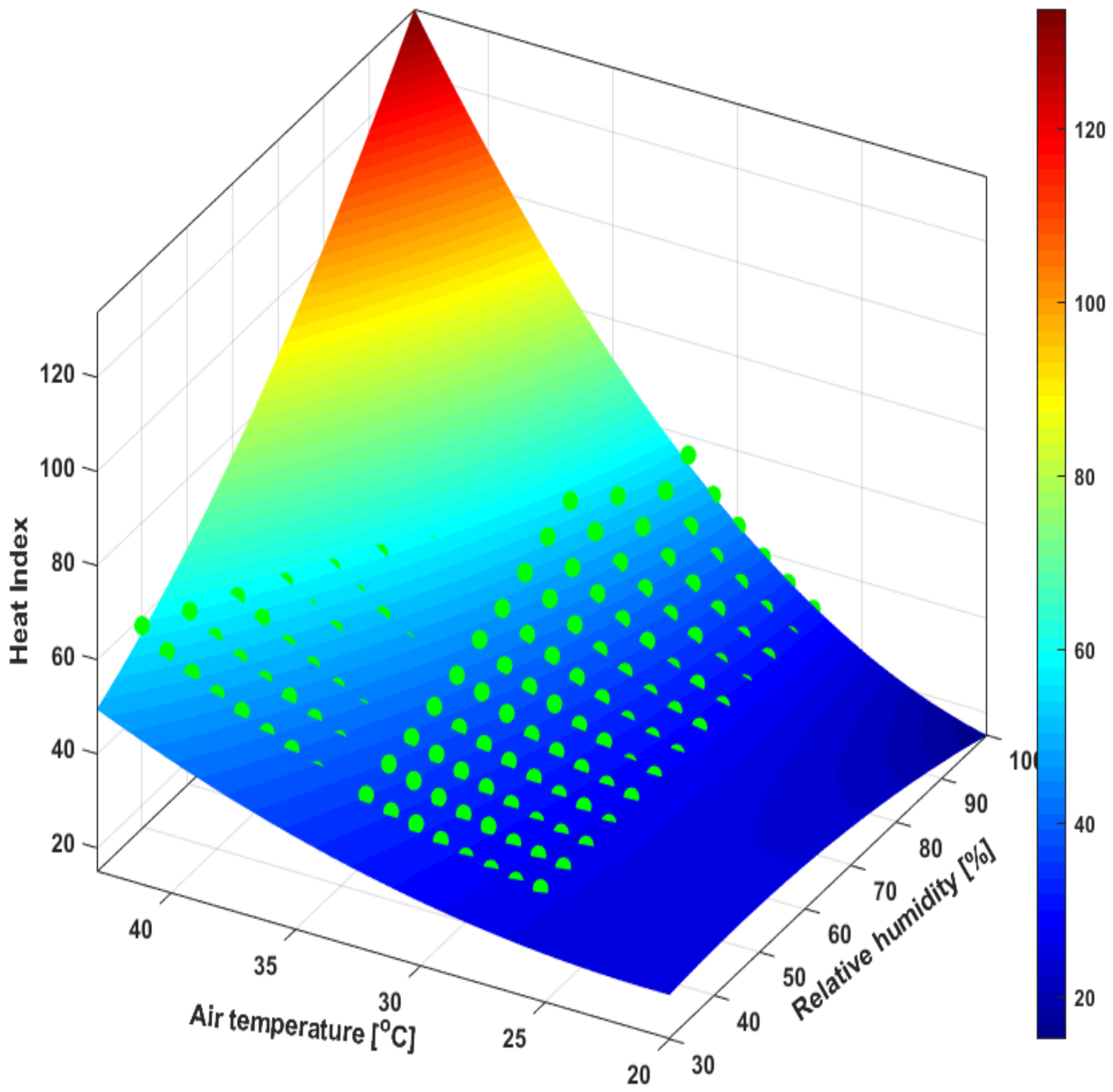
(Heat index model [38]). The heat index (HI) model requires a 2-dimensional input vector, where $\mathbf{x}\in {\mathbb{R}}^2$ is the 2 climatic variables (air temperature and relative humidity) [38,39]. The heat index model $g\left(\mathbf{x},\xi \right):{\mathbb{R}}^2⟼\mathbb{R}$ is tabulated (look-up table), which means that for different combinations of air temperature and relative humidity values, the value of the HI can be expressed.

2.1. Surrogate Model for OTC Indices

Since there are a myriad of OTC indices, it would be a good idea to develop a single model which is able to represent all the models in the same way. While this model might be an approximation of the original OTC model, it will posses the following desirable properties:

• A single model which is able to accurately represent many OTC models;
• A single model with the ability to develop a mathematically tractable model for the spatial risk model.

To achieve this goal, we now present the concept of a surrogate model.

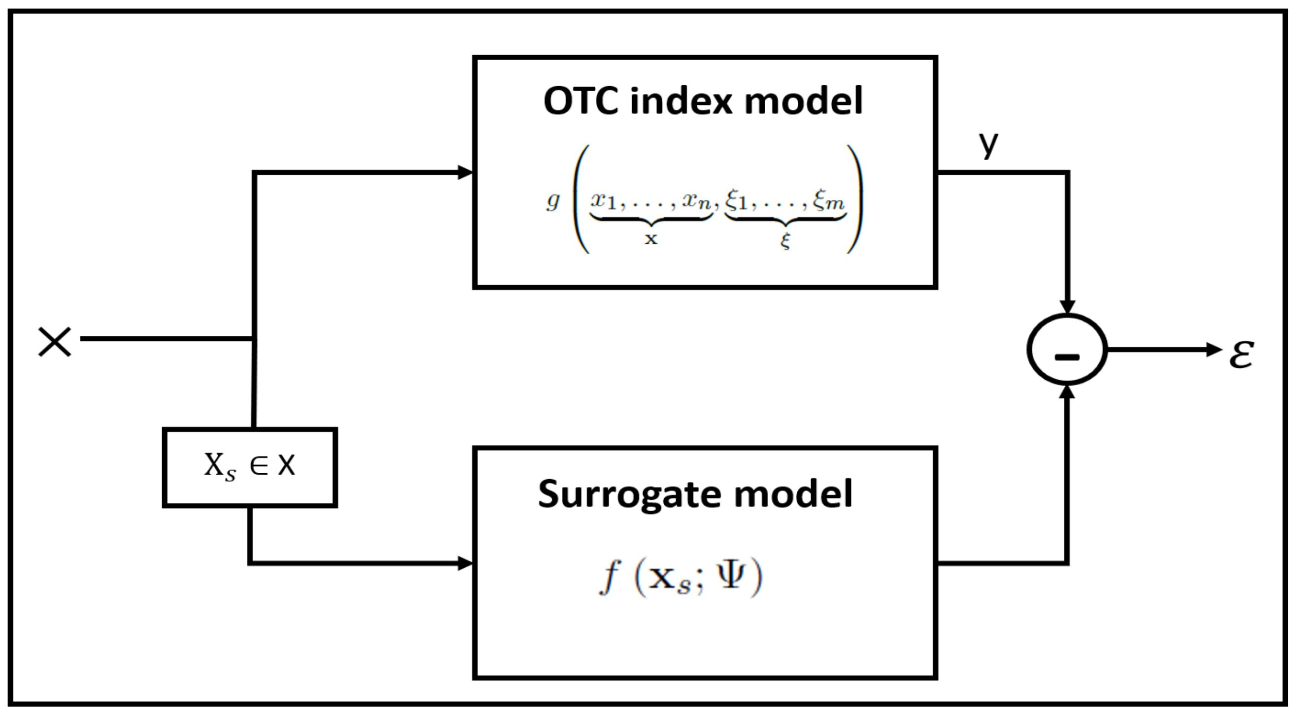
Definition 2

(Generic surrogate OTC index model). The generic surrogate OTC index model, $f\left({\mathbf{x}}_s;\Psi \right)$, of the generic OTC index model (See Definition 1), $g\left(\mathbf{x},\xi \right)$, is given by:

$$\begin{array}{c}\hfill \begin{array}{cc}\hfill y& =g\left(\mathbf{x},\xi \right)\hfill \\ \hfill & =f\left({\mathbf{x}}_s;\Psi \right)+ϵ,\hfill \end{array}\end{array}$$

(1)

where ${\mathbf{x}}_s\in {\mathbb{R}}^m\subset \mathbf{x}$, $m\le n$, Ψ is a vector of model parameters, and $ϵ\sim \mathcal{N}\left(\mu ,{\sigma }_{ϵ}^2\right)$ is a normal random variable accounting for the mismatch between the OTC index model $g\left(\mathbf{x},\xi \right)$ and the surrogate model $f\left({\mathbf{x}}_s;\Psi \right)$. The model is depicted in Figure 2.

Next, we define the specific family of regression models, $f\left({\mathbf{x}}_s;\Psi \right)$, which will be used for the generic surrogate OTC index model and is based on a second-order polynomial regression with coefficient interactions.

Definition 3

(Surrogate OTC index model via 2-order (quadratic) polynomial). The generic surrogate OTC index model is modeled as a 2-order (quadratic) polynomial regression, given by:

$$\begin{array}{c}\hfill \begin{array}{cc}\hfill f\left({\mathbf{x}}_s;\Psi \right)& :=\sum _{i=1}^m\sum _{j=1}^m{\alpha }_{i,j}{x}_i{x}_j+\sum _{i=1}^m{\beta }_i{x}_i+c\hfill \\ \hfill & ={\mathbf{x}}_s^T\mathbf{Q}{\mathbf{x}}_s+{\mathbf{x}}_s^T\mathbf{q}+c,\hfill \end{array}\end{array}$$

(2)

where the second line is a compact vector notation defined as:

$$\begin{array}{c}\hfill \begin{array}{cc}\hfill \mathbf{Q}& :=\left[\begin{array}{ccc}{\alpha }_{1,1}& \cdots & \frac{{\alpha }_{1,m}}{2}\\ ⋮& \cdots & ⋮\\ \frac{{\alpha }_{1,m}}{2}& \cdots & {\alpha }_{m,m}\end{array}\right]\in {\mathbb{R}}^{m\times m},\hfill \\ \hfill \mathbf{q}& :=\left[\begin{array}{c}{\beta }_1\\ ⋮\\ {\beta }_m\end{array}\right]\in {\mathbb{R}}^m.\hfill \end{array}\end{array}$$

(3)

The model coefficients are grouped into $\Psi :=\left[{\alpha }_{1,1},\dots ,{\alpha }_{m,m},{\beta }_1,\dots ,{\beta }_m,c,{\sigma }_{ϵ}^2\right]\in {\mathbb{R}}^{\left(m^2+m+2\right)}$.

2.2. Estimation of Surrogate Model Coefficients

We now present the estimation procedure for the model coefficients $\Psi$. We use the maximum likelihood estimator (MLE), which calculates the values $\widehat{\Psi }$ that maximize the likelihood function$L\left(\mathit{y};\Psi \right)$ for a given dataset $\mathcal{D}:={\left\{{\mathbf{x}}_s^{\left(n\right)},y^{\left(n\right)}\right\}}_{n=1}^N$.

Lemma 1

(Estimation of surrogate model coefficients, $\tilde{\mathbf{q}},{\sigma }_{ϵ}^2$ ). The model parameters estimators are given by:

$$\begin{array}{c}\hfill \begin{array}{cc}\hfill \widehat{\tilde{\mathbf{q}}}& ={\left({\mathbf{X}}_s^T{\mathbf{X}}_s\right)}^{-1}{\mathbf{X}}_s^T\mathit{y},\hfill \\ \hfill {\widehat{\sigma }}_{ϵ}^2& =\frac{1}{n}\sum _{n=i}^n{\left(y^{\left(n\right)}-{\mathbf{X}}_s^{\left(n\right)}\widehat{\tilde{\mathbf{q}}}\right)}^2.\hfill \end{array}\end{array}$$

Proof. 

See Appendix A. □

Proposition 1

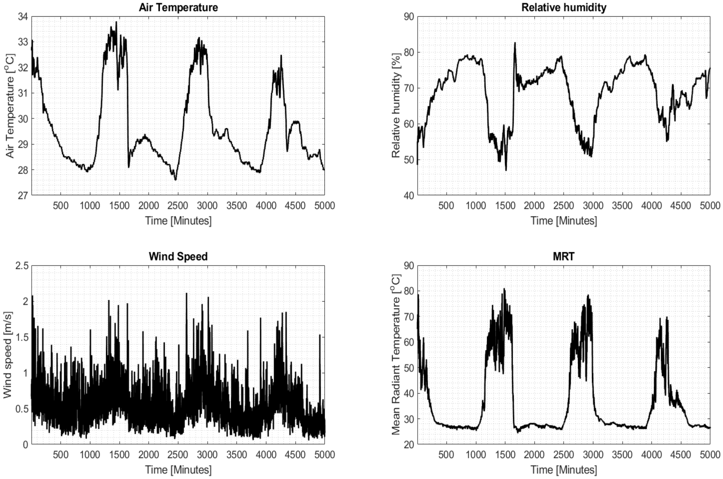
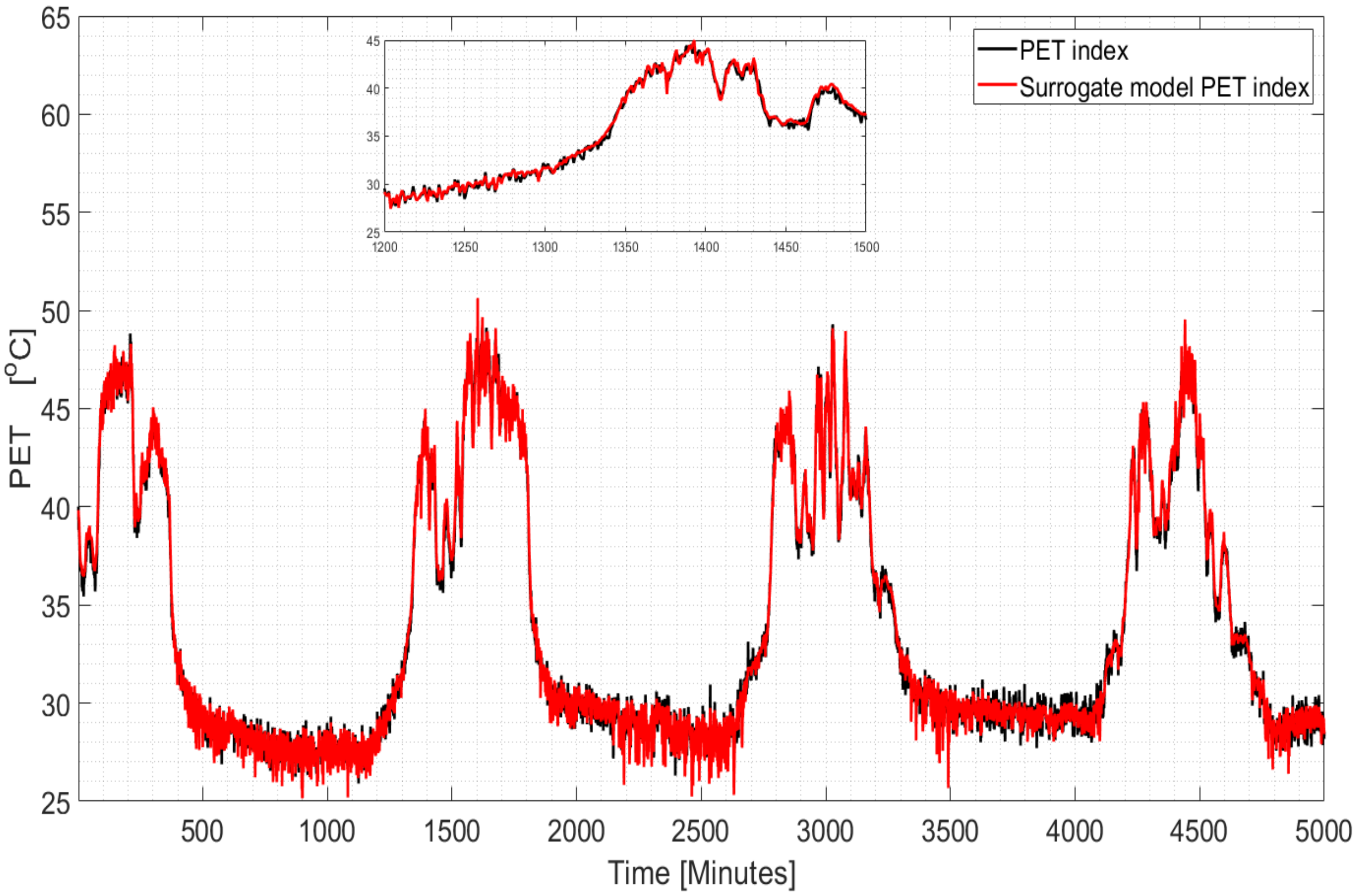
(OTC index estimation). Given the climatic variables ${\mathbf{x}}_s$, the estimated OTC index values are given by:

$$\begin{array}{c}\hfill \widehat{y}={\mathbf{x}}_s\widehat{\tilde{\mathbf{q}}},\end{array}$$

where the estimated model parameters $\widehat{\tilde{\mathbf{q}}}$ are presented in Lemma 1.

Example 3

(Surrogate model of the PET index). We present the performance of the OTC index surrogate model based on Proposition 1. We use a dataset which was collected in Singapore and contains the four climatic variables (the order of the vector is: MRT, AT, RH, and WS). The climatic variables are presented as time series in Figure 3. We then generated the six personal variables (age, sex, weight, height, metabolic activity level, and clothing level) using Monte Carlo draws. The PET index was calculated and used as a training set to estimate the parameters of the surrogate model as per Proposition 1. The time series of the true PET index values and the surrogate model-based one are presented in Figure 4. Clearly, the surrogate model provides very accurate estimates of the true PET values.

3. Statistical Properties of OTC Indices under Climate Model Uncertainty

In the previous section, we estimated the parameters of the surrogate model for the OTC index, where the data was provided by high-accuracy weather stations. In practice, we use a climate model to estimate the climatic variables in both space and time. Urban climate models, such as EnviMet, ANSYS Fluent for micro-scales or weather research forecast (WRF) for meso-scales, and other models, are physics-based models. Such models exhibit different levels of inaccuracy, which we generically define as uncertainty. We do not aim at distinguishing the different types of uncertainties; instead, we are only interested in the output accuracy of the climate model. We do not restrict the use to any specific climate model, but allow the usage of any model as long as the uncertainty has been quantified by the user, as in, for example, [40,41]. To this end, we model the overall behavior of the climate model as a “truth plus error” model, which is widely used [37]. As such, we assume that the true value of the physical phenomenon is ${\mathbf{x}}_s$, while the output of the climate model is given by ${\widehat{\mathbf{x}}}_s$. The discrepancy between the two is given by a RV $\zeta$, as is presented in the following definition.

Definition 4

(Imperfect climate model). The output variables of the climate model are modeled as an additive error model:

$$\begin{array}{c}\hfill \begin{array}{c}\hfill \underset{\begin{array}{c}“\mathit{true}”\mathit{climate}\\ \mathit{variable}\mathit{value}\end{array}}{\underbrace{x_i}}=\underset{\begin{array}{c}\mathit{estimated}\mathit{climate}\\ \mathit{variable}\mathit{value}\end{array}}{\underbrace{\widehat{x_i}}}+\underset{\begin{array}{c}\mathit{estimation}\\ \mathit{error}\end{array}}{\underbrace{{\zeta }_i}},i\in \left\{1,\dots ,m\right\},\end{array}\end{array}$$

(4)

where $x_i$ is the true climate variable value and $\widehat{x}$ is the climate variable estimate from the climate model. The term ${\zeta }_i$ represents the inaccuracy (estimation error) of the climate model. We further assume that the error term is temporally, spatially, as well as modally independent:

$$\begin{array}{c}\hfill \begin{array}{c}\hfill {\zeta }_i\stackrel{i.i.d}{\sim }\mathcal{N}\left(0,{\sigma }_{{\zeta }_i}^2\right).\end{array}\end{array}$$

(5)

The value ${\sigma }_{\zeta }^2$ depends on the accuracy of the climate model and can be calculated using multiple calibration procedures [42].

We express the collection of climate variables in a compact vector form, ${\mathbf{x}}_s:={\left[x_1,\dots ,x_m\right]}^T$, and express the climate model uncertainty as:

$$\begin{array}{c}\hfill \begin{array}{c}\hfill {\mathbf{x}}_s={\widehat{\mathbf{x}}}_s+\zeta ,\end{array}\end{array}$$

(6)

where $\zeta \sim \mathcal{MVN}\left(0,\mathsf{\Sigma }\right),$ and $\mathsf{\Sigma }$ is a diagonal matrix with elements ${\left\{{\sigma }_{{\zeta }_i}^2\right\}}_{i=1}^m$ on its main diagonal.

3.1. Joint Surrogate OTC Index and Climate Model

We now utilize the results from the previous section, integrate them with the climate model uncertainty, and derive the statistical properties of the OTC index while taking the climate model uncertainty into consideration.

Definition 5

(Surrogate model for OTC indices under climate model uncertainty). The surrogate model for OTC indices under climate model uncertainty is given by:

$$\begin{array}{c}\hfill \begin{array}{c}\hfill \left\{\begin{array}{cc}y\hfill & =f\left({\mathbf{x}}_s;\Psi \right)+ϵ,(OTCsurrogatemodel,Definition2)\hfill \\ f\left({\mathbf{x}}_s;\Psi \right)\hfill & :={\mathbf{x}}_s^T\mathbf{Q}{\mathbf{x}}_s+{\mathbf{x}}_s^T\mathbf{q}+c,(OTCsurrogateregressionmodel,Definition3)\hfill \\ {\mathbf{x}}_s\hfill & ={\widehat{\mathbf{x}}}_s+\zeta ,(Imperfectclimatemodel,Definition4)\hfill \end{array}\right.\end{array}\end{array}$$

where:

$$\begin{array}{c}\hfill \begin{array}{c}\hfill \left\{\begin{array}{cc}\hfill & \Psi :=\left[{\alpha }_{1,1},\dots ,{\alpha }_{m,m},{\beta }_1,\dots ,{\beta }_m,c\right],(Surrogatemodelparameters)\hfill \\ \hfill & ϵ\sim \mathcal{N}\left(0,{\sigma }_{ϵ}^2\right),(OTCsurrogatemodelerror)\hfill \\ \hfill & \zeta \sim \mathcal{MVN}\left(0,\mathsf{\Sigma }\right)(Climatemodeluncertainty)\hfill \end{array}\right.\end{array}\end{array}$$

3.2. Distribution of OTC Index under Climate Model Uncertainty

We now present the distribution of the OTC index under climate model uncertainty, where we condition (that is, assume to be known) the following two components:

• The estimated surrogate model parameters, $\widehat{\Psi },{\widehat{\sigma }}_{ϵ}^2$;
• The climate model estimated values ${\widehat{\mathbf{x}}}_s$ and the climate model estimation error $\mathsf{\Sigma }$.

The distribution is presented in the following.

Theorem 1

(Distribution of OTC index under climate model uncertainty). The OTC index value, y, follows a generalized chi-squared distribution as follows:

$$\begin{array}{c}\hfill y|{\widehat{\mathbf{x}}}_s;\widehat{\Psi },\mathsf{\Sigma }\sim {\tilde{\chi }}^2\left(\omega ,k,\lambda ,\mu ,s\right),\end{array}$$

where $\left\{\omega ,k,\lambda ,\mu ,s\right\}$ are defined in Appendix B.

Proof. 

See Appendix B. □

Now that we have derived the distribution of the OTC index, we present its statistical properties, which will be useful in the following section, where we develop the risk model. For notation tractability, we drop the conditioning on model parameters $\left({\widehat{\mathbf{x}}}_s,\widehat{\Psi },{\widehat{\sigma }}_{ϵ}^2,\sum \right)$, and it is understood that those parameters are known.

3.3. Statistical Properties of OTC Index under Climate Model Uncertainty

Here, we present some of the statistical properties of the OTC index which will be used in the following section, which include the mean and variance of the OTC index.

Proposition 2

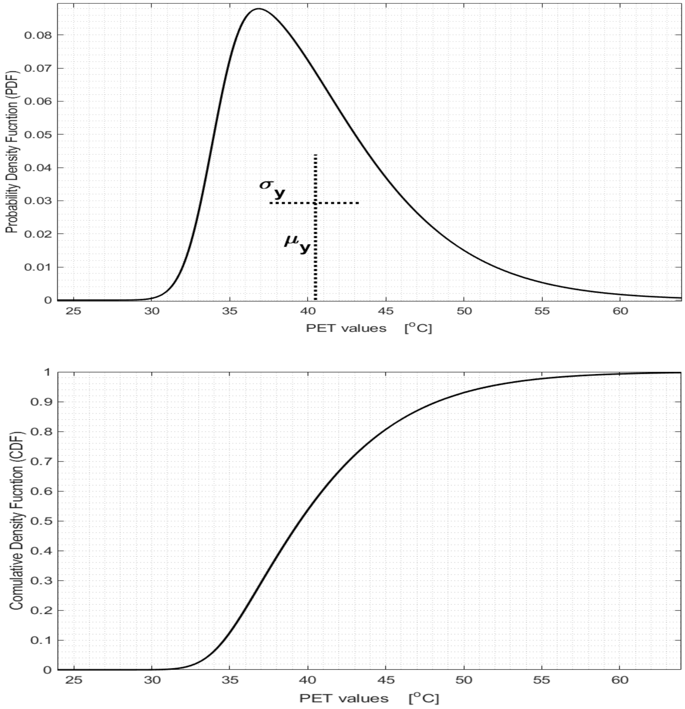
(Statistical properties of OTC index under climate model uncertainty). The mean and variance of the OTC index value, y, as presented in Theorem 1, are given by:

$$\begin{array}{cc}\hfill {\mu }_y& =\mathbb{E}\left[y\right]=\sum _{i\in {\lambda }_{\ne 0}}{\omega }_i\left(k_i+{\lambda }_i\right)+\mu ,\hfill \\ \hfill {\sigma }_y^2& =\mathbb{V}\mathrm{ar}\left[y\right]=2\sum _{i\in {\lambda }_{\ne 0}}{\omega }_i^2\left(k_i+2{\lambda }_i\right)+s^2.\hfill \end{array}$$

Example 4.

We now illustrate, in Figure 5, the result in Theorem 1 for the PET index. We set the estimated climatic variables to ${\widehat{\mathbf{x}}}_s={\left[50,25,80,1\right]}^T$ (the order of the vector is: MRT, AT, RH, and WS). We also present the mean and variance values as presented in Proposition 2.

3.4. Spatial-Temporal Representation of the OTC Index

Until now, we have considered the surrogate modeling of the OTC index based on the available climatic variables (perfect and imperfect). We now use those results and present the previous results, which are relevant to the domain of the climate model output, which is both spatial and temporal. The physical domain (site) is defined on some predefined spatial domain which is of interest to the designer, and a duration of time (usually a 24-h profile). To this end, we define the spatio-temporal space that the climate model is simulating:

• The spatial area is denoted by $\mathcal{Z}\subset {\mathbb{R}}^2$. Examples include a whole city or a residential neighborhood;
• The time duration of interest is denoted by $\mathcal{T}\subset \left[0,\infty \right)$. Examples include a whole year or a single day;
• The estimated climate values at location $\mathbf{z}\in \mathcal{Z},$ time $t\in \mathcal{T},$ are denoted in a similar manner to Equation (6), with the inclusion of spatial and temporal indicators ${\widehat{\mathbf{x}}}_s\left(\mathbf{z},t\right)$.

Based on these definitions, we can re-write the generic surrogate OTC index model of Definition 5, in both space and time, as:

$$\begin{array}{c}\hfill \begin{array}{c}\hfill \left\{\begin{array}{cc}y\left(\mathbf{z},t\right)\hfill & =f\left({\mathbf{x}}_s\left(\mathbf{z},t\right);\Psi \right)+ϵ\left(\mathbf{z},t\right),(\mathrm{Spatio}-\mathrm{temporal}\mathrm{OTC}\mathrm{index})\hfill \\ f\left({\mathbf{x}}_s\left(\mathbf{z},t\right);\Psi \right)\hfill & ={\mathbf{x}}_s^T\left(\mathbf{z},t\right)\mathbf{Q}{\mathbf{x}}_s\left(\mathbf{z},t\right)+{\mathbf{x}}_s^T\left(\mathbf{z},t\right)\mathbf{q}+c,(\mathrm{Spatio}-\mathrm{temporal}\mathrm{surrogate}\mathrm{model})\hfill \\ {\mathbf{x}}_s\left(\mathbf{z},t\right)\hfill & ={\widehat{\mathbf{x}}}_s\left(\mathbf{z},t\right)+\zeta \left(\mathbf{z},t\right),(\mathrm{Spatio}-\mathrm{temporal}\mathrm{climate}\mathrm{model})\hfill \end{array}\right.\end{array}\end{array}$$

As this set of equations depicts, there is one set of model parameters for the whole spatio-temporal domain, making our regression-based surrogate model parsimonious. It is important to note that while this set of equations reflects the spatio-temporal model, the parameters of the model that belong to the surrogate model are common and need be estimated once, based on the training dataset, which is described in Lemma 1. In addition, we can express the mean and variance, as per Proposition 2, as a function of the spatio-temporal domain: ${\mu }_y\left(\mathbf{z},t\right)$ and ${\sigma }_y^2\left(\mathbf{z},t\right)$.

In the following section, we utilize the surrogate model in order to derive spatial risk models.

4. Spatial Risk Models for OTC

In the previous sections, we derived the distribution of the OTC index under the climate model uncertainty. We now use those results in order to calculate the spatio-temporal risk that stems from the climatic conditions. Before we do that, we first need to understand that is meant by “risk measures”.

4.1. Risk Measures

Mathematically, a risk measure is a mapping from a class of random variables to the real line (i.e., $\mathbb{R}$). The properties of risk measures and the means for their application depend on the context of the problem and the requirements of the decision makers. Risk measures are valuable, as they translate the high-dimensional spatio-temporal climate model data into easy-to-understand real-valued numbers. Many developments have been derived over the last few decades. One important concept is known as coherent risk measures. The concept of the “coherence” of risk measures was introduced in the seminal paper of Artzner, and initiated a rigorous and axiomatic analysis of risk assessments. Under coherent risk measures theory, the mathematical properties of risk measures were derived from a set of four intuitive axioms: monotonicity, subadditivity, positive homogeneity, and translation invariance [43]. We now present the most basic definition of risk measures.

Definition 6

(Risk measure [44]). A risk measure is a function (mapping) of a random variable Y to the extended real line, $\overline{\mathbb{R}}:=\mathbb{R}\cup \left\{+\infty \right\}\cup \left\{-\infty \right\}$. That is, given a random variable $y\in \mathcal{Y}$, a risk measure is the mapping $\rho \left(y\right):\mathcal{Y}\to \overline{\mathbb{R}}.$

This definition is quite broad, and it is clear that there are infinite number of risk measures to choose from, since any combination of risk measures is, in itself, a risk measure, making the choice of a “good” risk measure complicated. One simple and intuitive choice of a risk measure is the mean-variance risk measure, which combines the expected value as well as its dispersion. This combinations is easy to follow and has been studied for many years since the seminal work of Markowitz on portfolio allocation [34].

Definition 7

(Mean-variance risk measure [44]). The mean-variance risk measure of a random variable Y is defined as:

$$\begin{array}{c}\hfill {\rho }_{MV}\left(y\right):=\mathbb{E}\left[y\right]+c\mathbb{V}\mathrm{ar}\left[y\right],\end{array}$$

where $c\ge 0$ is the risk aversion parameter and is a known constant.

The main idea of mean–variance models is to characterize the uncertain outcome by two scalar characteristics:

• The mean $\mathbb{E}\left[y\right]$, describing the expected outcome;
• The dispersion measure $\mathbb{V}\mathrm{ar}\left[y\right]$, which measures the uncertainty of the outcome.

A different risk measure that is widely used is the value-at-risk (VaR), which calculates the probability that the risk is above a pre-defined allowed level.

Definition 8

(Value-at-risk (VaR) [44]). The value-at-risk (VaR) of a random variable Y and a probability level $\alpha \in \left(0,1\right)$ is defined as the α-percentile of the distribution of y:

$$\begin{array}{c}\hfill \begin{array}{cc}\hfill {\rho }_{VaR}\left(y;\alpha \right)& =F_Y^{-1}\left(\alpha \right)\hfill \\ \hfill & :=\underset{t\in \mathbb{R}}{inf}\left\{t:F_Y\left(t\right)\ge \alpha \right\},\hfill \end{array}\end{array}$$

where $F_Y$ is the CDF of y.

The VaR is simply the $\alpha$-quantile of the R.V. y, and is the most widely used risk measure in insurance applications, where one is interested in modeling the losses due to extreme events [45]. Before we analyze the risk measures of the OTC index, we present a simple illustration of the aforementioned risk measures.

Example 5

(Scalar risk measures). Consider a R.V. Y, which follows a Gamma distribution, i.e., $Y\sim \Gamma \left(k,\theta \right)$, where we set $k=2$ and $\theta =3$. Then, $\mathbb{E}\left[y\right]=k\theta =6$ and $\mathbb{V}\mathrm{ar}\left[y\right]=k{\theta }^2=18$. This is depicted in Figure 6, in addition to the VaR measure for $\alpha =0.9$: ${\rho }_{VaR}\left(y;\alpha =0.9\right)=F_Y^{-1}\left(0.9\right)=11.67$.

Now that we have defined the notion of risk measures, we are ready to extend this definition to the case where many OTC values are aggregated either spatially, temporally, or both.

4.2. Aggregate Spatial Risk Models for OTC

Spatial-temporal aggregation refers to the aggregation of all the OTC values of the elementary units (e.g., squares of 300 × 300 m${}^2$) in a specified region and over a specified period of time. This operator enables us to analyze a whole region of interest and compare it to another one. There are different aggregation functions which we could consider. Generically, an aggregation function is a mapping from a high-dimensional space ${\mathcal{Z}}_a\times {\mathcal{T}}_a\subseteq \mathcal{Z}\times \mathcal{T}$ to the real-line: $\mathbb{T}\left(\mathit{y}\right):{\mathbb{R}}^{\left|{\mathcal{Z}}_a\right|}\times {\mathbb{R}}^{\left|{\mathcal{T}}_a\right|}\to \mathbb{R}$. We now define the generic representation of aggregated risk; see more details on the topic in [46].

Definition 9

(Generic aggregate OTC risk). The generic aggregate risk measure is defined as:

$$\begin{array}{c}\hfill \begin{array}{cc}\hfill \overline{\rho }\left(\mathit{y}\left(\mathbf{z}\in {\mathcal{Z}}_a,t\in {\mathcal{T}}_a\right)\right)& :=\rho \left(\mathbb{T}\left(\mathit{y}\left(\mathbf{z}\in {\mathcal{Z}}_a,t\in {\mathcal{T}}_a\right)\right)\right),\hfill \end{array}\end{array}$$

where $\rho \left(y\right):\mathcal{Y}\to \overline{\mathbb{R}}$ (see Definition 6), $\mathbb{T}\left(y\right):{\mathbb{R}}^{\left|{\mathcal{Z}}_a\right|}\times {\mathbb{R}}^{\left|{\mathcal{T}}_a\right|}\to \mathbb{R}$ is an aggregation function, and ${\mathcal{Z}}_a\subseteq \mathcal{Z}$ and ${\mathcal{T}}_a\subseteq \mathcal{T}$ are the spatial and temporal subsets, respectively.

There are many different choices of the aggregation function, including the summation, average, minimum, maximum, and more. The aggregation function acts as a statistical summary of the spatio-temporal data. In this work, we concentrate on the intuitive choice of a summation function, defined next.

Definition 10

(Spatio-temporal aggregate risk (STAR) measure for OTC). The Spatio-temporal aggregate risk (STAR) measure is defined as:

$$\begin{array}{c}\hfill \begin{array}{cc}\hfill \overline{\rho }\left(\mathit{y}\left(\mathbf{z}\in {\mathcal{Z}}_a,t\in {\mathcal{T}}_a\right)\right)& :=\rho \left(\overline{y}\right),\hfill \end{array}\end{array}$$

where $\overline{y}:={\displaystyle \sum _{\mathbf{z}\in {\mathcal{Z}}_a}}{\displaystyle \sum _{t\in {\mathcal{T}}_a}}y\left(\mathbf{z},t\right)$ and ${\mathcal{Z}}_a\subseteq \mathcal{Z}$ and ${\mathcal{T}}_a\subseteq \mathcal{T}$.

We now derive the distribution of $\overline{y}$, which is obtained by summing independent generalized chi-squared RVs and is presented in the following Theorem.

Theorem 2

(Statistical properties of STAR). The STAR is a random variable $\overline{y}$, as defined in Proposition 4, and follows a generalized chi-squared distribution as follows:

$$\begin{array}{c}\hfill \overline{y}\sim {\tilde{\chi }}^2\left(\omega ,k,m,s\right),\end{array}$$

where $\left\{\omega ,k,m,s\right\}$ are defined in Appendix C. The mean and variance can be calculated similarly to Proposition 2.

Proof. 

See Appendix C. □

This result is important since it tells us than when we aggregate the spatial-temporal values, the sum of the values follows a generalized chi-squared distribution, which we have already analyzed, and therefore, makes a very convenient mathematical structure.

We express two risk measures of STAR, as per Definitions 7 and 8.

Theorem 3

(Statistical properties of STAR). The STAR is a random variable $\overline{y}$, which follows a generalized chi-squared distribution as follows:

$$\begin{array}{c}\hfill \overline{y}\sim {\tilde{\chi }}^2\left(\omega ,k,m,s\right),\end{array}$$

where $\left\{\omega ,k,m,s\right\}$ are defined in Appendix C.

Proposition 3

(STAR under mean-variance risk measure). Under the mean-variance risk measure, we have that the STAR is given by:

$$\begin{array}{c}\hfill \begin{array}{cc}\hfill {\overline{\rho }}_{MV}\left(\mathit{y}\left(\mathbf{z}\in {\mathcal{Z}}_a,t\in {\mathcal{T}}_a\right)\right)& =\mathbb{E}\left[\overline{y}\right]+c\mathbb{V}\mathrm{ar}\left[\overline{y}\right]\hfill \\ \hfill & =\mathbb{E}\left[\sum _{\mathbf{z}\in {\mathcal{Z}}_a}\sum _{t\in {\mathcal{T}}_a}y\left(\mathbf{z},t\right)\right]+c\mathbb{V}\mathrm{ar}\left[\sum _{\mathbf{z}\in {\mathcal{Z}}_a}\sum _{t\in {\mathcal{T}}_a}y\left(\mathbf{z},t\right)\right]\hfill \\ \hfill & =\sum _{\mathbf{z}\in {\mathcal{Z}}_a}\sum _{t\in {\mathcal{T}}_a}\mathbb{E}\left[y\left(\mathbf{z},t\right)\right]+c\sum _{\mathbf{z}\in {\mathcal{Z}}_a}\sum _{t\in {\mathcal{T}}_a}\mathbb{V}\mathrm{ar}\left[y\left(\mathbf{z},t\right)\right]\hfill \\ \hfill & =\sum _{\mathbf{z}\in {\mathcal{Z}}_a}\sum _{t\in {\mathcal{T}}_a}{\mu }_y\left(\mathbf{z},t\right)+c\sum _{\mathbf{z}\in {\mathcal{Z}}_a}\sum _{t\in {\mathcal{T}}_a}{\sigma }_y^2\left(\mathbf{z},t\right),\hfill \end{array}\end{array}$$

where ${\mu }_y\left(\mathbf{z},t\right)$ and ${\sigma }_y^2\left(\mathbf{z},t\right)$ can be calculated according to Proposition 2.

Proposition 4

(STAR under VaR risk measure). Under the VaR risk measure, we have that the STAR is given by:

$$\begin{array}{c}\hfill \begin{array}{cc}\hfill {\overline{\rho }}_{Var}\left(\mathit{y}\left(\mathbf{z}\in {\mathcal{Z}}_a,t\in {\mathcal{T}}_a\right)\right)& :={\rho }_{Var}\left(\sum _{\mathbf{z}\in {\mathcal{Z}}_a}\sum _{t\in {\mathcal{T}}_a}y\left(\mathbf{z},t\right)\right)\hfill \\ \hfill & ={\rho }_{Var}\left(\overline{y}\right)\hfill \\ \hfill & =F_{\overline{Y}}^{-1}\left(\alpha \right),\hfill \end{array}\end{array}$$

where $F_{\overline{Y}}$ is the CDF of $\overline{y}$.

5. Spatial Resource Allocation for OTC Improvement

Now that we have shown how to derive the spatial risk measures, we turn our attention to developing a spatial resource allocation framework which uses the previous results. In many practical problems, the DM (say, a government agency) is given a sum of money to invest in improving the OTC throughout a pre-specified region. This could be a city, a canton, or even a country; see [15] for an example where the cost of implementation was integrated into the overall objective function. Here, we extend this concept to allocating the resources to multiple spatial sites. A practical and common approach for allocating the money is to partition the physical domain into a finite number of regions, and allocate the money to each region according to some decision mechanism. For example, in [47], the authors presented a list of more than 80 heat-mitigation strategies which could be implemented. The strategies aiming at improving OTC levels are grouped into seven categories: vegetation, urban geometry, water bodies, materials, shading, transport, and energy. In [48], the authors evaluated the costs and benefits of different mitigation strategies. They concentrated on the impact of two aspects: the electrification of vehicle fleets and district cooling. They used the PET as the OTC index and showed how to combine economic costs with thermal comfort jointly as the objective function. To decide which strategy to implement in each spatial sector, a decision mechanism needs to be formulated and solved. This decision mechanism, which we call the spatial resource allocation, is presented next.

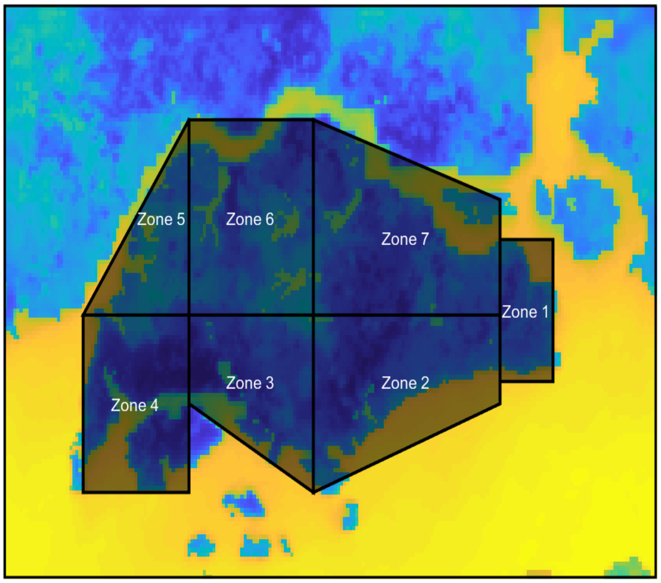
Let K, be the number of spatial regions; we then partition the spatial domain $\mathcal{Z}$ into K disjoint regions, such that:

$$\begin{array}{c}\hfill \begin{array}{cc}\hfill \mathcal{Z}& =\bigcup _{k=1}^K{\mathcal{Z}}_a^k,\left(\mathrm{exhaustive}\right)\hfill \\ \hfill \varphi & ={\mathcal{Z}}_a^l\bigcap {\mathcal{Z}}_a^j,\forall l\ne j,\left(\mathrm{exclusive}\right),\hfill \end{array}\end{array}$$

(7)

where $\varphi$ denotes the empty set.

Each region will be allocated a portion of the money, denoted by ${\left\{{\alpha }_k\in {\mathbb{R}}_{+}\right\}}_{k=1}^K$, such that ${\displaystyle \sum _{k=1}^K}{\alpha }_k=1$, meaning that all the money will be used. Next, we define how much a region would benefit if an $\alpha$ amount was invested in it. To do so, we need to introduce a function which quantifies this improvement (through some physical and technological intervention). In many practical cases, we are interested in reducing the OTC index levels. This is relevant to many hot countries and regions, and we, therefore, interpret the improvement as a reduction of OTC levels; in the following, we define the impact of the intervention in such a way. In cases where the DM is interested in increasing the OTC index levels (e.g., cold regions), the next definition can be trivially adapted to accommodate for such cases.

Definition 11

(Marginal OTC intervention impact). The marginal OTC intervention impact is defined as the change (i.e., reduction) in OTC level which results from an intervention of level α when the non-intervention level (i.e., baseline) is $\overline{y}$. That is, if the current OTC level is $\overline{y}$, then the α-impact is defined as follows:

$$\begin{array}{c}\hfill \begin{array}{c}\hfill \Delta \left(\overline{y},\alpha \right):=\underset{\mathit{baseline}}{\underbrace{\overline{y}}}-\underset{\mathit{Improvement}}{\underbrace{\mathsf{\Lambda }\left(\overline{y},\alpha \right)}},\end{array}\end{array}$$

where $\mathsf{\Lambda }\left(\overline{y},\alpha \right)$ is the utility function, which provides a measure of improvement. Then, its risk measure is given by $\rho \left(\Delta \left(\overline{y},\alpha \right)\right)$.

A practical example of a utility function will be presented in more detail in Example 6, but we keep the notion of a utility function generic, and it is up to the DM to use the appropriate utility function. Now that we have defined the $\alpha$-impact on the STAR value $\overline{y}$, we move to defining the resource allocation problem, where we are interested in finding the set of weights such that the aggregate risk is minimized.

Definition 12

(Optimal resource allocation for spatial risk minimization). The optimal spatial resource allocation is given by minimizing the aggregate STAR measure, after the intervention has been implemented, as follows:

$$\begin{array}{c}\hfill \begin{array}{cc}\hfill \left\{{\alpha }_1,\cdots ,{\alpha }_K\right\}& =\underset{\alpha }{arg\; min}\sum _{k=1}^K\rho \left(\Delta \left({\overline{y}}_k,{\alpha }_k\right)\right),\hfill \\ \hfill s.t.& \sum _{k=1}^K{\alpha }_k=1.\hfill \end{array}\end{array}$$

In the following, we concentrate on the mean-variance risk measure, which complies with the celebrated Markowitz optimal portfolio allocation theory [33,34]. To this end, we need to calculate the first two moments of $\Delta \left(\overline{y},{\alpha }_k\right).$ This is difficult to obtain in cases where the utility function is non-linear. Therefore, we present here a general method to approximate the first two moments in such cases by using the Taylor series expansion, presented next.

Proposition 5

(Calculation of moments via Taylor series expansion). The first and second moments of the marginal OTC intervention impact in Definition 11 can be approximated using Taylor series expansion, presented next.

Expectation of$\Delta \left(\overline{y},\alpha \right):$

$$\begin{array}{c}\hfill \begin{array}{cc}\hfill \mathbb{E}\left[\Delta \left(\overline{y},\alpha \right)\right]& \approx \mathbb{E}\left[\Delta \left({\mu }_{\overline{y}},\alpha \right)+{\Delta }^{\prime }\left({\mu }_{\overline{y}},\alpha \right)\left(\overline{y}-{\mu }_{\overline{y}}\right)+\frac{1}{2}{\Delta }^{\prime \prime }\left({\mu }_{\overline{y}},\alpha \right){\left(\overline{y}-{\mu }_{\overline{y}}\right)}^2\right]\hfill \\ \hfill & =\Delta \left({\mu }_{\overline{y}},\alpha \right)+\frac{1}{2}{\Delta }^{\prime \prime }\left({\mu }_{\overline{y}},\alpha \right){\sigma }_{\overline{y}}^2,\hfill \end{array}\end{array}$$

(8)

where $\mathbb{E}\left[\overline{y}-{\mu }_{\overline{y}}\right]=0$, so that the second term disappears and $\mathbb{E}\left[{\left(\overline{y}-{\mu }_{\overline{y}}\right)}^2\right]={\sigma }_{\overline{y}}^2.$

Variance of$\Delta \left(\overline{y},\alpha \right):$

$$\begin{array}{c}\hfill \begin{array}{cc}\hfill \mathbb{V}\mathrm{ar}\left[\Delta \left(\overline{y},\alpha \right)\right]& \approx {\left({\Delta }^{\prime }\left({\mu }_{\overline{y}},\alpha \right)\right)}^2{\sigma }_{\overline{y}}^2,\hfill \end{array}\end{array}$$

(9)

where ${\Delta }^{\prime }\left({\mu }_{\overline{y}},\alpha \right),{\Delta }^{\prime \prime }\left({\mu }_{\overline{y}},\alpha \right)$ are the first and second derivatives of $\Delta \left({\mu }_{\overline{y}},\alpha \right)$, with respect to ${\mu }_{\overline{y}}$.

We are now ready to present the optimal spatial resource allocation optimization problem.

Lemma 2

(Optimal spatial resource allocation under the mean-variance risk measure). The optimal spatial resource allocation under the mean-variance risk measure is given by:

$$\begin{array}{c}\hfill \begin{array}{cc}\hfill \left\{{\alpha }_1,\cdots ,{\alpha }_K\right\}& =\underset{\alpha }{arg\; min}\sum _{k=1}^K\left(\underset{\approx \mathbb{E}\left[\Delta \left(\overline{y},\alpha \right)\right]}{\underbrace{\Delta \left({\mu }_{\overline{y}},\alpha \right)+\frac{1}{2}{\Delta }^{\prime \prime }\left({\mu }_{\overline{y}},\alpha \right){\sigma }_{\overline{y}}^2}}+c\underset{\approx \mathbb{V}\mathrm{ar}\left[\Delta \left(\overline{y},\alpha \right)\right]}{\underbrace{{\left({\Delta }^{\prime }\left({\mu }_{\overline{y}},\alpha \right)\right)}^2{\sigma }_{\overline{y}}^2}}\right).\hfill \\ \hfill s.t.& \sum _{k=1}^K{\alpha }_k=1.\hfill \end{array}\end{array}$$

Solving the optimization problem in Lemma 2 is not difficult, since we assume that the utility function is concave. This means that the objective function is concave, and so is the constraint set, and the optimization problem can be easily solved via Lagrange multiplier [49].

To illustrate this result, we now provide an example which shows how to implement the spatial resource allocation for the simplest case, that is, when the spatial domain contains two regions ($K=2$). Since the optimization problem, in this case, is only two-dimensional, we are able to visualize this scenario.

Example 6

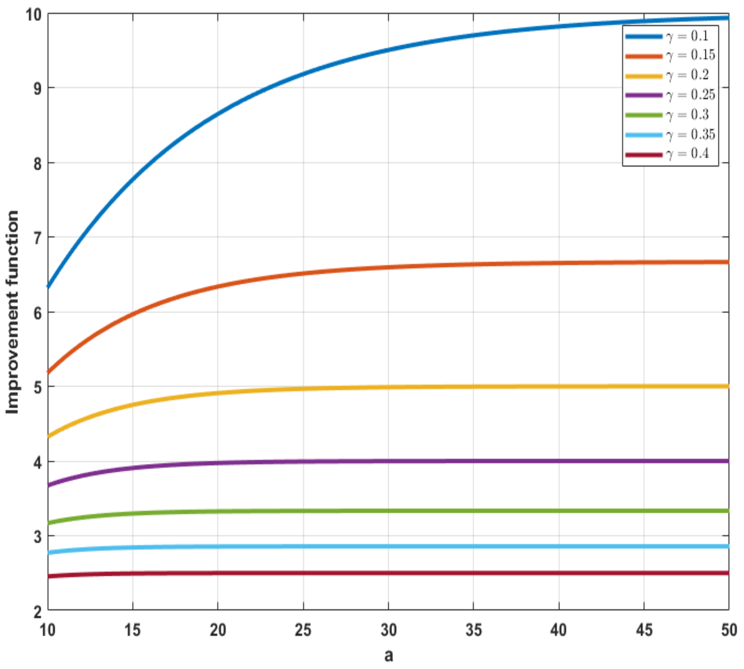
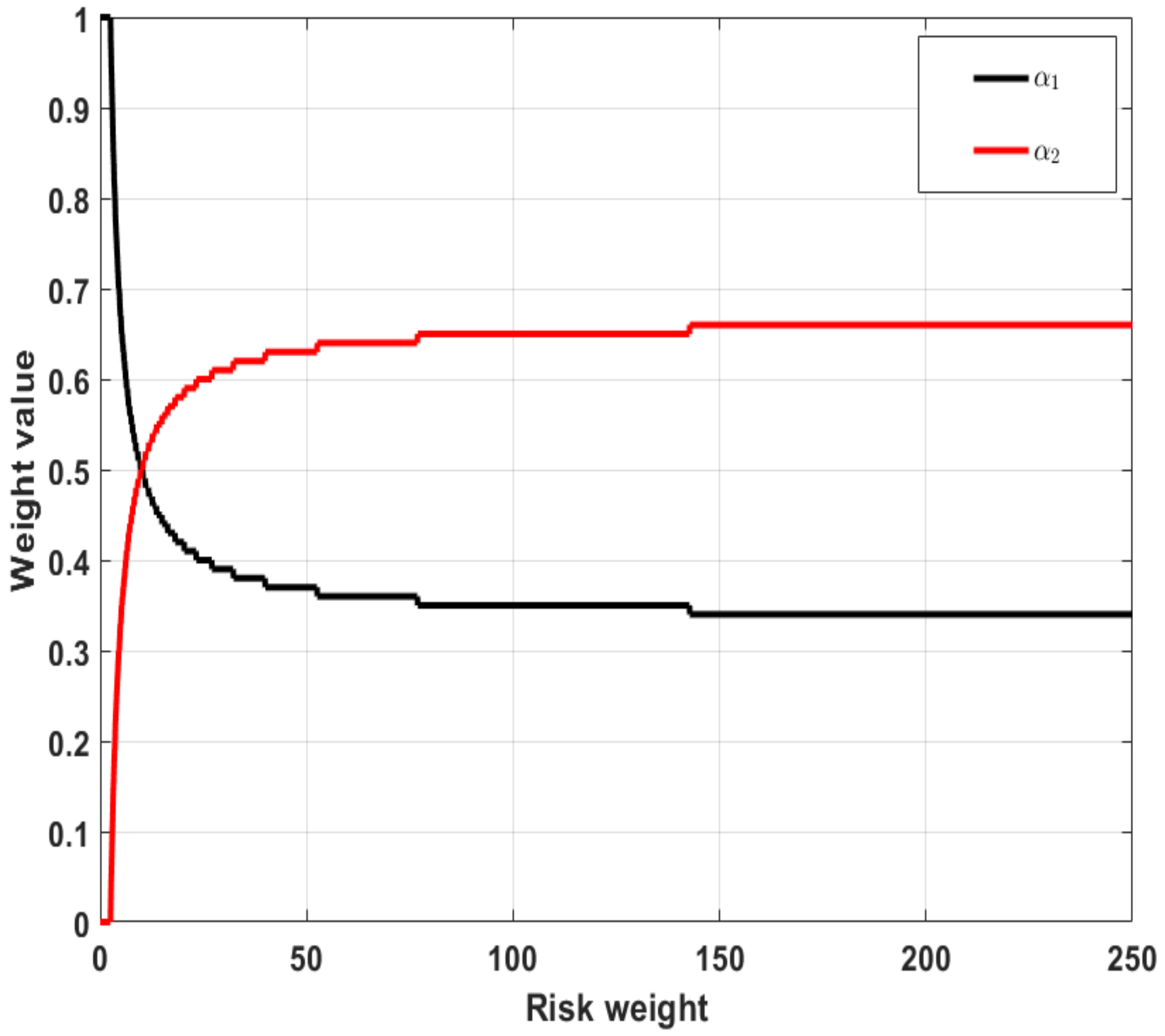
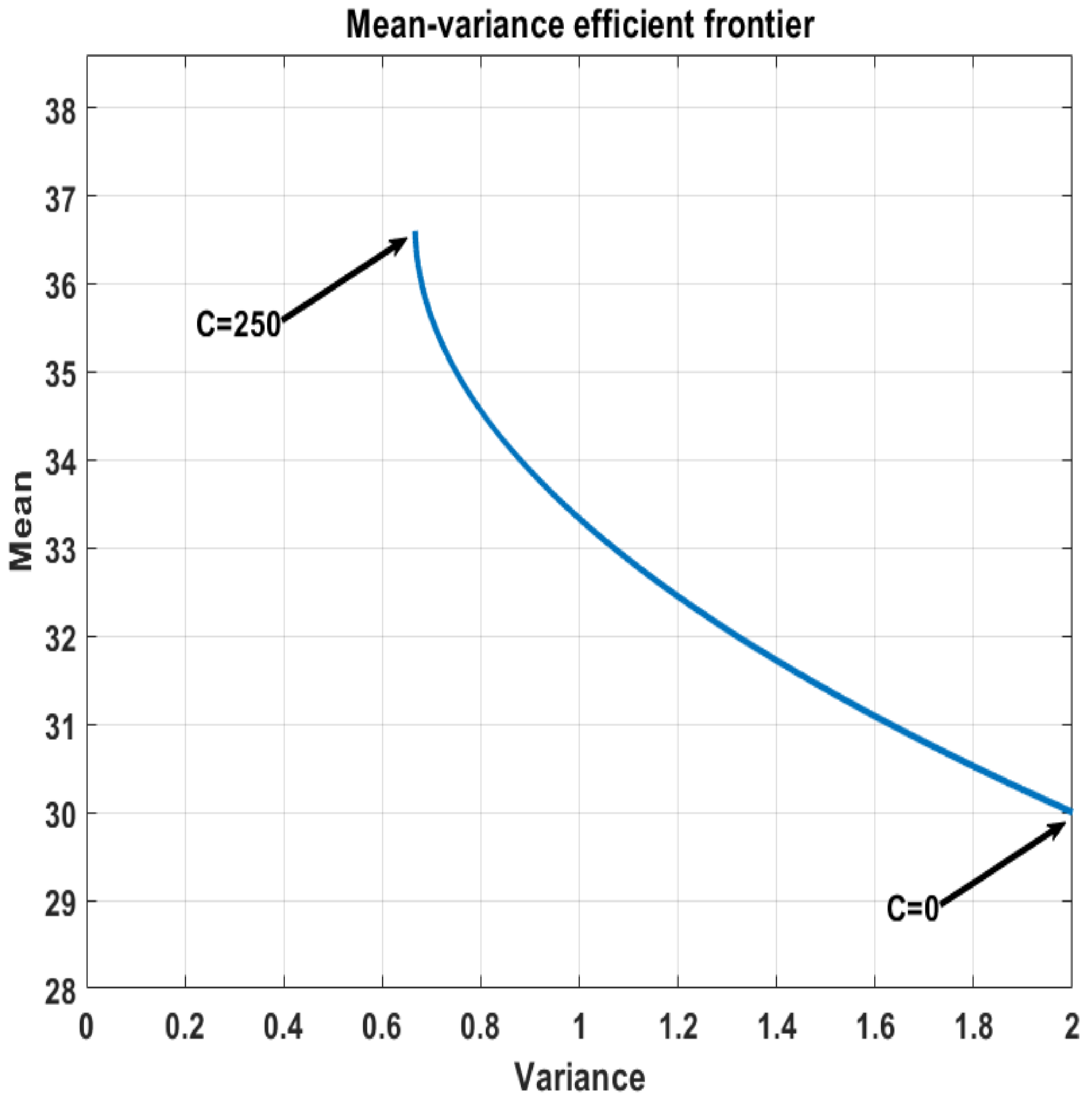
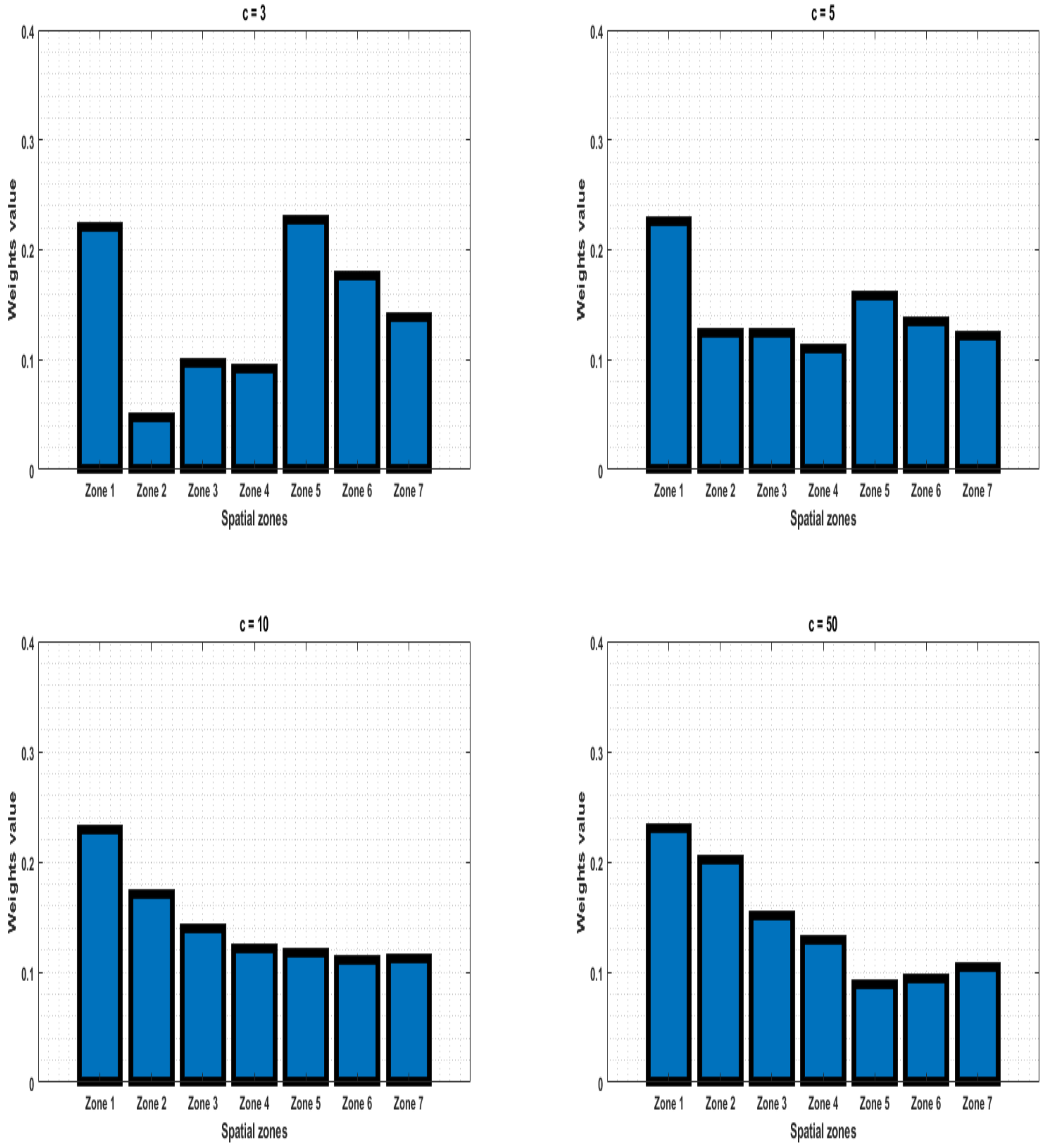
(Optimal spatial resource allocation for two regions). We assume that the utility function is given by the following exponential function:

$$\begin{array}{c}\hfill \mathsf{\Lambda }\left(a;\alpha ,\gamma \right)=\alpha \left(1-exp\left(-\gamma a\right)\right)/\gamma ,\end{array}$$

where $\gamma \ne 0$ is a known constant. This is depicted in Figure 7 and is widely used due to its flexibility by varying the values of γ.

Its first and second derivatives, with respect to the input variable ${}^{‘}{a}^{’}$, are given by:

$$\begin{array}{c}\hfill \begin{array}{cc}\hfill {\mathsf{\Lambda }}^{\prime }\left(a,b;\gamma \right)& =\alpha exp\left(-\gamma a\right),\hfill \\ \hfill {\mathsf{\Lambda }}^{\prime \prime }\left(a,b;\gamma \right)& =-\alpha \gamma exp\left(-\gamma a\right).\hfill \end{array}\end{array}$$

(10)

Then, we have that the objective function in Lemma 2 is given by:

$$\begin{array}{c}\hfill \begin{array}{cc}\hfill \Delta \left({\mu }_{\overline{y}},\alpha \right)+\frac{1}{2}{\Delta }^{\prime \prime }\left({\mu }_{\overline{y}},\alpha \right){\sigma }_{\overline{y}}^2+c{\left({\Delta }^{\prime }\left({\mu }_{\overline{y}},\alpha \right)\right)}^2{\sigma }_{\overline{y}}^2& =\overline{y}-\alpha \left(1-exp\left(-\gamma {\mu }_{\overline{y}}\right)\right)/\gamma \hfill \\ \hfill & -\frac{1}{2}\alpha \gamma exp\left(-\gamma {\mu }_{\overline{y}}\right){\sigma }_{\overline{y}}^2\hfill \\ \hfill & +c{\left(\alpha exp\left(-\gamma {\mu }_{\overline{y}}\right)\right)}^2{\sigma }_{\overline{y}}^2.\hfill \end{array}\end{array}$$

Let us assume that $K=2$; then, their mean and variance values are $\left({\mu }_{{\overline{y}}_1},{\sigma }_{{\overline{y}}_1}^2\right)$ and $\left({\mu }_{{\overline{y}}_2},{\sigma }_{{\overline{y}}_2}^2\right)$, respectively. The optimal allocation optimization problem reads:

$$\begin{array}{c}\hfill \begin{array}{cc}\hfill \left\{{\alpha }_1,{\alpha }_2\right\}=\underset{\alpha }{arg\; min}& ({\mu }_{{\overline{y}}_1}-{\alpha }_1\left(1-exp\left(-\gamma {\mu }_{{\overline{y}}_1}\right)\right)/\gamma \hfill \\ \hfill & -\frac{1}{2}{\alpha }_1\gamma exp\left(-\gamma {\mu }_{{\overline{y}}_1}\right){\sigma }_{{\overline{y}}_1}^2\hfill \\ \hfill & +c{\left({\alpha }_{1}exp\left(-\gamma {\mu }_{{\overline{y}}_1}\right)\right)}^2{\sigma }_{{\overline{y}}_1}^2\hfill \\ \hfill & +{\mu }_{{\overline{y}}_2}-{\alpha }_2\left(1-exp\left(-\gamma {\mu }_{{\overline{y}}_2}\right)\right)/\gamma \hfill \\ \hfill & -\frac{1}{2}{\alpha }_2\gamma exp\left(-\gamma {\mu }_{{\overline{y}}_2}\right){\sigma }_{{\overline{y}}_2}^2\hfill \\ \hfill & +c{\left({\alpha }_{2}exp\left(-\gamma {\mu }_{{\overline{y}}_2}\right)\right)}^2{\sigma }_{{\overline{y}}_2}^2),\hfill \\ \hfill s.t.& {\alpha }_1+{\alpha }_2=1.\hfill \end{array}\end{array}$$

(11)

This optimization can be easily solved by setting ${\alpha }_2=1-{\alpha }_1$, taking the derivative, setting it to 0, and solving for ${\alpha }_1$. In this example, we set $\left\{{\mu }_{{\overline{y}}_1}=40,{\sigma }_{{\overline{y}}_1}^2=2,{\mu }_{{\overline{y}}_2}=30,{\sigma }_{{\overline{y}}_2}^2=1\right\}.$ The values of ${\alpha }_1$ for different values of risk weight (c in Lemma 2) are presented in Figure 8. In Figure 9, we present the mean-variance plot under the optimal solution for different values of c; see Definition 12.

Figure 7. The exponential utility function with $\gamma =\left\{0.1,0.15,0.2,0.25,0.3,0.35,0.4\right\}$.

Figure 7. The exponential utility function with $\gamma =\left\{0.1,0.15,0.2,0.25,0.3,0.35,0.4\right\}$.

Figure 8. Illustration of the optimal choice of the weights for different risk attitudes ($c\in \left(0,250\right)$).

Figure 8. Illustration of the optimal choice of the weights for different risk attitudes ($c\in \left(0,250\right)$).

Figure 9. Illustration of the mean and variance under the optimal choice of the weights for different risk attitudes ($c\in \left(0,250\right)$).

Figure 9. Illustration of the mean and variance under the optimal choice of the weights for different risk attitudes ($c\in \left(0,250\right)$).

6. Results: Spatial OTC Risk and Resource Allocation in Singapore

In this section, we demonstrate how to apply the framework for a practical problem of resource allocation for OTC improvement in Singapore. We first provide details of the climate model we use and quantify its uncertainty. We then move to developing the surrogate model for the heat index, which is a widely used OTC index. Finally we will show how the resource allocation scheme we developed is applied for this practical setting.

6.1. Climate Model Simulation Set-Up

The climate model we use is the multilayer urban canopy model (MLUCM) embedded in WRF version $3.8.1$, and it incorporates building effect parametrization (BEP) and the building energy model (BEM) [50,51]. The details of the model set-up can be found in [40,52].

6.2. Validation and Uncertainty Estimation of Climate Model

In order to calculate the uncertainty of the WRF simulations according to Definition 4, we conducted a validation procedure where the output of the WRF variables were compared against the network of 15 meteorological stations provided by the Meteorological Service Singapore (MSS). The WRF simulations and meteorological stations’ observations were averaged over 24 h for the entire month of April 2016. We now present the calculation of the uncertainty for the air temperature and relative humidity, since they are required for the OTC index we shall use.

6.2.1. Air Temperature Estimation

We compared the air temperature WRF simulations against observations from weather stations at 2-m height. The results show that the simulated and observed means agree during early hours of the day and during nighttime, except for the rural stations, while during the afternoon, the means deviate and the temperature is either under or over the predicted, except for rural stations. Negative bias exists for the urban stations and positive bias values are observed for the rural stations. The mean average error (MAE) is 0.6 °C and the root mean squared error (RMSE) is 0.74 °C.

6.2.2. Relative Humidity Estimation

The RH is underestimated by the model during early morning and nighttime for most of the stations. A negative bias exits for both urban and rural stations, indicating the under-prediction of relative humidity. The mean average error (MAE) for all stations was $6\%$, and the root mean squared error (RMSE) was $6.61\%$. We can, therefore, express the bi-variate climatic model for AT and RH as per Definition 4 as follows:

$$\begin{array}{c}\hfill \begin{array}{cc}\hfill x_1\left(\mathbf{z},t\right)& ={\widehat{x}}_1\left(\mathbf{z},t\right)+{\zeta }_1\left(\mathbf{z},t\right),(\mathrm{Air}\mathrm{temperature}),\hfill \\ \hfill x_2\left(\mathbf{z},t\right)& ={\widehat{x}}_2\left(\mathbf{z},t\right)+{\zeta }_2\left(\mathbf{z},t\right),(\mathrm{Relative}\mathrm{humidity}),\hfill \end{array}\end{array}$$

where ${\widehat{x}}_1\left(\mathbf{z},t\right),{\widehat{x}}_2\left(\mathbf{z},t\right)$ are the WRF estimated AT and RH values, respectively. The model errors are given by:

$$\begin{array}{c}\hfill \begin{array}{cc}\hfill {\zeta }_1\left(\mathbf{z},t\right)& \stackrel{\mathrm{i}.\mathrm{i}.\mathrm{d}}{\sim }\mathcal{N}\left(0.6,0.5476\right),\hfill \\ \hfill {\zeta }_2\left(\mathbf{z},t\right)& \stackrel{\mathrm{i}.\mathrm{i}.\mathrm{d}}{\sim }\mathcal{N}\left(6,43.6\right).\hfill \end{array}\end{array}$$

6.3. Surrogate Model for the Heat Index

In this study, we use the heat index as the OTC index; see Example 2 for details. For the training data, we used the tabulated values of [38,39]. We then used the surrogate model developed in Section 2 to interpolate the HI for the missing values. This is presented in Figure 10, where the green dots represent the known tabulated values, and the surface represents all possible combinations of input–output HI values.

Once the surrogate model has been estimated, we can use it for estimating the HI values, based on the WRF simulations for Singapore on a spatio-temporal domain. In Figure 11, we present the spatial heat maps of the time averaged AT, RH, and HI.

6.4. Spatial Resource Allocation

We now turn our attention to the resource allocation problem, which was presented in Section 5. First, we spatially partitioned Singapore into seven zones; see Figure 12. This partition is only used for illustration purposes, and in practice, should be determined by the DM according to their criteria.

We then used the results of Theorem 3 to derive the statistical properties of each zone. In particular, we used the same concept of Proposition 2 to calculate the mean and variance of each zone separately; these are presented in Figure 13.

We used the utility function in Example 6, solved the optimization problem of Lemma 2, and obtained the seven allocation weights. It is important to note that the choice of the free parameter c is at the discretion of the DM. In Figure 14, we present the solution of the optimization problem and the values of the seven weights for different choices of $c=\left[3,5,10,50\right]$. To understand those results, we need to remember that c controls the balance between the mean and the variance values; see Definition 7. The larger c is, the more high values of variance are penalized by the objective function, which shifts the allocation of the resources towards Zones 2, 3, and 4, since their variance values are smaller relative to the other zones. Clearly, for $c=0$, the variance would not be taken into account, and only the mean would be considered. In this case, Zone 5 would receive a weight of one, since its mean value is the smallest.

7. Conclusions

In this paper, we developed a rigorous mathematical framework and a new class of statistical models for spatial risk models. We addressed the modeling and quantification of the spatial risk profile of an urban area from an OTC perspective using the concept of a surrogate model. We then estimated the spatial risk profile and used that to develop a new framework for resource allocations for OTC level reduction. We presented the concept of spatio-temporal aggregate risk (STAR) measures and derived their statistical properties. Finally, using the STAR measures, we developed a new algorithm for spatial resource allocation that is useful for practical decision making. We provided a practical example and illustrated how the framework we developed could be used in practice in the case of the large-scale area of Singapore using the WRF climate model. The results show the importance of the framework and its ability to mitigate and reduce the urban climate risk. The framework can be implemented and used by DMs in order to optimally utilize their resources. Future work includes the development of the framework into a tool which can be used by DMs via a simple and intuitive interface.