Evaluating Probability Distribution Functions for the Standardized Precipitation Evapotranspiration Index over Ethiopia

Abstract

Drought indices are used to identify and monitor drought events. The standardized precipitation evapotranspiration index (SPEI) is a widely used index based on accumulated water balance. There is, however, no broad consensus on which probability distribution is the most appropriate for water balances. This issue is investigated for Ethiopia using 125 meteorological stations spread across the country. Based on long-term series, a selection was made among the generalized extreme value, Pearson type 3, and generalized logistics (Genlog) distributions. Additionally, the effect of using actual, instead of potential, evapotranspiration and a limited amount of data (10, 15, 20, and 25 years) is explored. Genlog is found to be the best distribution for all accumulation periods. Furthermore, there is a considerable difference amongst the SPEI values estimated from the three distributions on the identification of extreme wet or extreme dry periods. Next, there are significant differences between standardized precipitation actual evapotranspiration index (SPAEI) and SPEI, signifying the importance of drought index selection for proper drought monitoring. Finally, time series of 20 or 25 years of data lead to almost similar SPEI values to those estimated using more than 30 years of data, so could potentially be used to assess drought in Ethiopia.

1. Introduction

Drought can be defined as a temporary decrease in water availability over an extended period. Since there is a wide range of drought definitions, depending on the impact, drought studies are a multifaceted or multidisciplinary area of research. Furthermore, drought prediction is difficult since rainfall is difficult to predict [1]. Moreover, it possesses a major threat to the livelihoods and multiple economic sectors worldwide, especially those largely dependent on subsistence agriculture. Drought incidents are mostly followed by socioeconomic impact (reduced income of farmers, increased heat strokes, etc.). The African continent is well known to be affected by drought, and specifically, Ethiopia is usually given as an example of impactful drought in Africa [2,3,4,5,6], despite being called the “water tower of Africa”. For instance, in 2015, a severe drought struck Northern Ethiopia. According to the Emergency Events Database (EM-DAT—https://www.emdat.be/, last accessed on 6 June 2021), in the past 100 years, Ethiopia suffered from 402,367 drought-related casualties, and around 70 million people are directly or indirectly affected by drought.

Droughts can be categorized as meteorological, agricultural, and/or hydrological droughts. Meteorological droughts are defined as a below-average precipitation/water balance (precipitation–evapotranspiration) value. Agricultural droughts occur when there is below-normal crop yield due to the decrease of water in the root zone. Finally, hydrological droughts are characterized by reduced water availability in hydrological bodies (e.g., groundwater, surface water bodies, etc.). Generally, the timescale over which precipitation deficits/water balances accumulate is vital to differentiate these drought types. For example, agricultural droughts have a much shorter timescale than hydrological droughts (droughts in groundwater or surface water bodies). In this paper, timescales ranging from 1 to 24 months are assessed, thereby covering most drought types.

The severity of droughts is usually expressed using drought indices. Among the many, the Standardized Precipitation Index (SPI) [7] and the Standardized Precipitation Evaporation Index (SPEI) [8] are widely used. Individual drought indices for different durations could also be combined to obtain an overall drought assessment [9]. Furthermore, drought indices are useful for identifying the intensity and duration of drought [10]. Each index has its benefits and limitations. Thus, a comparison is needed to identify indices that suit a given case or basin.

Both SPI and SPEI are probability-based indices that consider the distribution of precipitation and water balance, respectively. Based on 11 gauging stations located at different places in the world, in Ref. [8], the log-logistic distribution was found to be appropriate for the water balance (and to estimate the SPEI). However, recent studies have shown that other distributions are also adequate to fit the water balance [11,12]. While literature agrees that SPI fitting is best performed with the gamma distribution, a universally optimal distribution for SPEI is currently not encountered. In Ref. [11], for instance, it was found that the generalized extreme value (GEV) distribution fits the water balance better than the log-logistic distribution or the Pearson type 3 (PE3) distribution for Europe. On the other hand, Ref. [12] showed that PE3 outperforms the other distribution types, especially for shorter timescales, while GEV performs well for longer timescales for most parts of India. The findings of Ref. [13] that are based on 541 stations in China are in accordance with Ref. [8] but also claim that the PE3 and the GEV distributions describe the water balance well. It is to be noted that the log-logistic distribution is a two-parameter family, but to allow for negative values for SPEI, Ref. [8] added a third location-parameter. As noted in Ref. [11], this extended distribution is mathematically equivalent to the (three-parameter) generalized logistic distribution (Genlog).

Recently, the use of actual evapotranspiration instead of potential evapotranspiration for estimating the drought index has received more attention [14,15,16,17,18]. It has the advantage of representing the actual drought characteristics while considering land and vegetation variability. Hence, it is intended to assess the use of AET instead of PET which also has the potential to indicate the uncertainty in the drought index estimation by different inputs.

The time series length-dependence for drought analysis over Ethiopia was investigated in Ref. [19], but their focus was on assessing drought categories, and the assessment did not consider less than 30 years of data. In addition, research on the SPI values estimated using shorter and longer time series of global datasets were assessed for China [20]. Their analysis revealed that 17 years of data is sufficient to evaluate drought using either in situ or global datasets. Such research is vital mainly for developing countries that generally lack long observed precipitation time series.

The main focus of this paper is to assess which of the three candidate distributions (Genlog, GEV, PE3) are the most appropriate for the water balance in Ethiopia and to calculate SPEI accurately, which otherwise may lead to inappropriate drought monitoring. In addition, the relative difference between the SPEI estimations is compared by visual inspection and the Nash–Sutcliffe efficiency (NSE) coefficient. Finally, since gauging stations in Ethiopia are scarce and the available data length is short, comparison is made between the SPEI values estimated using short time series of precipitation data against those calculated using the complete series (benchmark data).

2. Materials and Methods

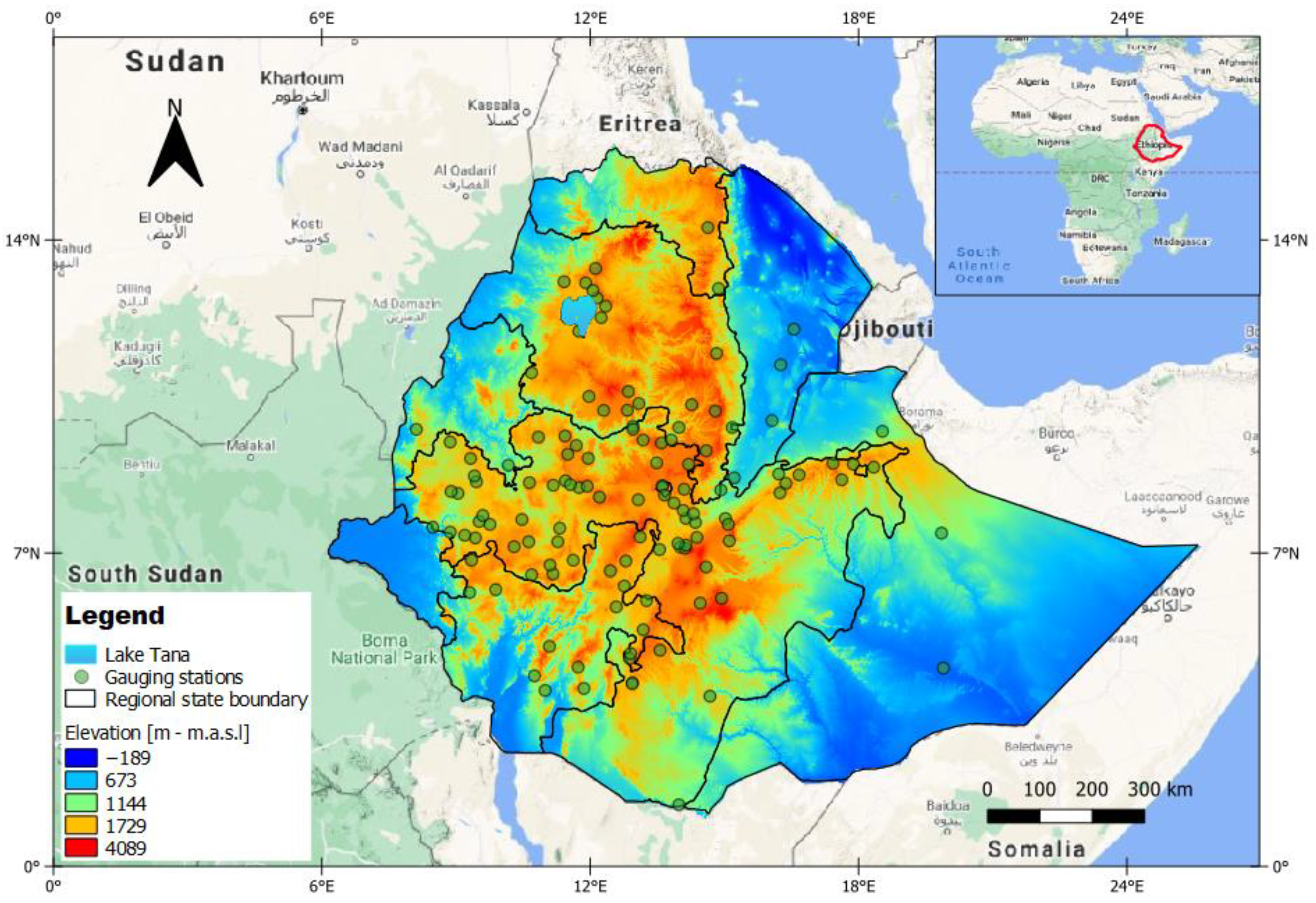
2.1. Study Area

The study area is located in Ethiopia, an eastern African country with a population of around 112 million (The World Bank; https://www.worldbank.org/en/home—last accessed on 4 June 2021). The Ethiopian climate is dry in the southeastern and northeastern parts of the country and wet in the country’s central, western, and southern regions. Mountainous areas range from the west and central to the northern part of the country. The precipitation has two main seasonal variations, where August to September are the wettest months, while December to April are the driest months. The spatiotemporal rainfall patterns are highly inhomogeneous due to the complex orography and convective nature of rainfall [21]. Moreover, the decadal variability of Ethiopian rainfall is known to be significant [22,23]. On the other hand, long-term series indicate either no trend [24] or a drying signal [25], while future model projections indicate a drying trend over the Ethiopian Highlands [26]. The country is well known for catastrophic drought events, as several incidents have resulted in the loss of human lives. Between 1973 and 1975 especially, more than 200,000 people have died due to starvation, malnutrition, and related diseases [27].

2.2. Climatic Data

Daily precipitation data from 273 gauging stations were obtained from the National Meteorology Agency of Ethiopia (NMA), and monthly aggregated precipitation values are used for the analysis. Out of the 273 gauging stations, the number of missing daily precipitation data was substantial. Hence, missing values are replaced using the CHIRPS (Climate Hazards Group InfraRed Precipitation with Station data) observational dataset [28]. Since this dataset started in 1981, it was decided to limit our analysis from 1981 onwards. The ending dates vary from station to station, but the total length of time series is longer than 30 years. Additionally only time series with less than ten years of missing data are considered, and we eventually found 125 stations that met these criteria (Figure 1).

According to Ref. [29], the CHIRPS observational dataset represents the precipitation in the Upper Blue Nile (UBN) better than other existing datasets, such as the Precipitation Estimation from Remotely Sensed Information using Artificial Neural Networks (PERSIANN), African Rainfall Climatology and Time-series (TARCAT) v2.0, Tropical Rainfall Measuring Mission (TRMM), and Africa Rainfall Estimate Climatology version 2 (ARC 2.0). A similar assessment of CHIRPS, ARC2, and TAMSAT by [30] for the Eastern Africa region showed the superior performance of CHIRPS.

Before using these values, multiplicative bias correction is applied on the CHIRPS dataset using the available gauging station data. Temperature data is obtained from ERA5 [31] at the nearest grid point of each gauging stations that are analyzed. ERA5 was recently compared with gridded observations and ERA-Interim over Africa [32]. It was shown that, despite persistent biases over the Ethiopian Highlands, ERA5 clearly reduced climatological biases with respect to ERA-Interim. Persistent biases may also arise due to the mismatch in spatial scales between ERA5 and stations observations that gives rise to large observational representativity errors in the orographically complex region. For further analysis, Table S1 in Supplementary Material lists the historical droughts since 1981 that are taken as a reference for selecting historical drought periods (EM-DAT https://www.emdat.be/, last accessed on 6 June 2021).

2.3. Standardized Precipitation Evapotranspiration Index (SPEI)

There are several methods to estimate potential evapotranspiration (PET), and they give different estimations. Since the Penman–Monteith method [33] requires several meteorological input variables that are difficult to obtain (e.g., solar radiation, wind speed, relative humidity, etc.), it is usually customary to use approximations such as the Thornthwaite equation [34], which only requires monthly mean temperature. However, this method has its own limitations, such as the overestimation of PET in tropical areas [35], and different SPEI values compared to those estimated using other PET estimation methods [36]. The difference between precipitation and PET (estimated using the method of Thornthwaite) is assumed to be the water balance at those stations.

After estimating the water balance, these values are aggregated into different timescales (1-, 3-, 6-, 9-, 12-, and 24-month accumulation periods are considered). The candidate distribution function is fitted to these aggregated values and transforms them to standard normally distributed values. The different drought index categories (see Table S2 in Supplementary Material) correspond to the degree of deviation from mean conditions (i.e., SPEI = 0). For our analysis, SPEI values are limited to vary between −3 and 3, as extreme values may be inaccurately determined [11,37]. Values less than −3 and above 3 are assigned −3 and 3, respectively. The SCI package is used to estimate the SPEI values using the three distribution functions [38].

2.4. Standardized Precipitation Actual Evapotranspiration Index (SPAEI)

The use of actual evapotranspiration can be better representative than PET to characterize some drought aspects (such as assessing the impact of evapotranspiration and land use and/or vegetation impact on drought). The Global Land Evaporation Amsterdam Model—GLEAM v3.5a [39,40]—database is used to estimate PET using the Priestley and Taylor equation. AET is calculated by multiplying PET with a stress factor, obtained from microwave observations of the vegetation optical depth (VOD), which is used as an approximation of the vegetation water content. The VOD is based on observations from different microwave satellite sensors [40]. The GLEAM dataset has been successfully validated worldwide [40] and over Africa specifically in Ref. [41] where it is recommended to be used for drought studies.

2.5. Probability Distribution Functions

The three considered candidate probability distribution functions, each featuring three parameters, are as follows:

• Pearson type III (PE3)

PE3 is commonly used in the field of hydrology and specifically for flood frequency analysis. It is a three-parameter distribution similar to a two-parameter gamma distribution (Γ), except that it has a location parameter (c) in addition to scale (β) and shape (α) parameters. The location parameter is useful for SPEI estimation as the water balance is not bounded by 0, as the deficit can lead to a water balance below zero. The PE3 distribution is represented by the following probability density function [42].

$$\mathrm{f}\left(\mathrm{x}\right)=\frac{1}{\mathsf{\beta }\mathsf{\Gamma }\left(\mathsf{\alpha }\right)}{\left(\frac{\mathrm{x}-\mathrm{c}}{\mathsf{\beta }}\right)}^{\mathsf{\alpha }-1}{\exp }^{-\left(\frac{\mathrm{x}-\mathrm{c}}{\mathsf{\beta }}\right)},\mathrm{where}\mathsf{\alpha }>0,\mathsf{\beta }>0\mathrm{and}0<\mathrm{c}<\mathrm{x}$$

(1)

• Generalized extreme value (GEV) distribution

The GEV distribution constitutes a family of continuous probability distributions proposed in extreme value theory [43,44]. It has been commonly applied for extreme events such as drought and flooding. This is given by

$$\mathrm{f}\left(\mathrm{x}\right)=\{\begin{array}{l}\left(\frac{1}{\mathsf{\sigma }}\right){\left(1+\mathsf{\xi }\mathrm{z}\right)}^{-\frac{1}{\mathsf{\xi }}-1}{\mathrm{e}}^{-{\left(1+\mathsf{\xi }\mathrm{z}\right)}^{-\frac{1}{\mathsf{\xi }}}}, \mathsf{\xi }\ne 0\\ 1+\mathsf{\xi }\mathrm{z}>0 \\ \left(\frac{1}{\mathsf{\sigma }}\right){\mathrm{e}}^{-\mathrm{z}-{\mathrm{e}}^{-\mathrm{z}}}, \mathsf{\xi }=0\end{array}$$

(2)

$$\mathrm{z}=\frac{\mathrm{x}-\mathsf{\mu }}{\mathsf{\sigma }}$$

where $\mathsf{\mu }$, $\mathsf{\sigma },$ and $\mathsf{\xi }$ are the location, scale, and shape parameters, respectively.

• Generalized logistic (Genlog) distribution

Genlog is usually used to model precipitation and streamflow and is of the form [45]

$$\mathrm{f}\left(\mathrm{x}\right)=\{\begin{array}{ll}& \mathsf{\kappa }\ne 0,\mathrm{z}=\frac{\log \left(1-\frac{\mathsf{\kappa }\left(\mathrm{x}-{\mathsf{\xi }}_{\mathrm{g}}\right)}{\mathsf{\alpha }}\right)}{-\mathsf{\kappa }}\\ \frac{\exp \left(-\left(1-\mathsf{\kappa }\right)\mathrm{z}\right)}{\mathsf{\alpha }{\left(1+\exp \left(-\mathrm{z}\right)\right)}^2}& \\ & \mathsf{\kappa }=0,\mathrm{z}=\frac{\mathrm{x}-{\mathsf{\xi }}_{\mathrm{g}}}{{\mathsf{\alpha }}_{\mathrm{g}}}\end{array}$$

(3)

$$-\infty <\mathrm{x}<\infty$$

where ξ_g, α_g, and κ are the location, scale, and shape parameters, respectively.

2.6. Distribution Fitting Using Shorter Time Series Data

The total time series data are reduced into a series of consecutive 10, 15, 20, and 25 years of data in order to assess the suitability of the three distributions to fit shorter length time series. Those years are selected by a one-month moving window where one full time series data will contain multiple m years-long data, where m is the short time series length (10, 15, 20, and 25). For example, 10/15/20 or 25 continuous years are selected starting from January and until the next m years. The next dataset will be generated starting from February until the next m years, and this continues until the full time series is used. This is performed for each station and each moving window separately. After selecting those time series, a comparison is made between SPEI estimated from shorter time series to those estimated using the benchmark data. Note that the benchmark data is subject to uncertainty, but, generally, it is the recommended data length for drought analysis. Furthermore, as an example, the most drought-hit period is selected (i.e., with the highest number of historical droughts) for inspecting the difference among the SPEI values estimated using 10, 15, 20, and 25 years of data.

2.7. Evaluating Distribution Functions and the SPEI Values

2.7.1. The Goodness-of-Fit Test (GOF)

The Kolmogorov–Smirnov (KS) and the Anderson–Darling test (AD) assess the goodness-of-fit (GOF) [46]. AD attributes more weight to the tails of the distribution while KS assesses the general fit [47]. If the test statistics value (A² or $\Delta$) is higher than a critical value, then the null hypothesis that the data comes from a specific distribution is rejected. Critical values are not always available in a closed analytical form, but they can be approximated using Monte Carlo simulation for a given distribution and sample size [48,49,50]. The AD statistic is given by

$${\mathrm{A}}^2=-\mathrm{n}-\frac{1}{\mathrm{n}}{\displaystyle \sum }_{\mathrm{i}=1}^{\mathrm{n}}\left(2\mathrm{i}-1\right)\left[{\mathrm{logF}}_{\mathrm{i}}+\log \left\{1-{\mathrm{F}}_{\mathrm{n}+1-\mathrm{i}}\right\}\right]$$

(4)

where F is the cumulative distribution function (while f in Section 2.5 is the corresponding density function) with data samples (x₁,x₂, …, x_n) with sample size n.

The KS statistic is given by

$$\Delta =\max \left|{\mathrm{F}}_{\left(\mathrm{t},\mathrm{i}\right)}-{\mathrm{F}}_{\left(\mathrm{e},\mathrm{i}\right)}\right|$$

(5)

where ${\mathrm{F}}_{\left(\mathrm{t},\mathrm{i}\right)}$ and ${\mathrm{F}}_{\left(\mathrm{e},\mathrm{i}\right)}$ are theoretical and empirical cumulative distribution function values at time step i of a specific distribution, respectively.

The rejection frequency for each statistical test is calculated at a 5% significance level for 12 months per gauging station divided by the total number of distribution fittings. The total number of distribution fittings corresponds to 125 gauging stations multiplied by 12 distribution fittings per gauging station. The R-package fitdistrplus is used to perform the GOF tests [51].

Whenever the distribution fitting with maximum likelihood (MLE) method fails (which may happen with short datasets or data points that fall outside the distribution domain), SPEI is calculated using initial parameter estimations from L-moments using the lmomco package in R [52]. Thus, it is crucial to assess the estimated SPEI values, hence, the Shapiro–Wilk test (SW) is used, which is equivalent to the classical GOF tests [11]. That is, in the estimation of SPEI, the transformation of the cumulative distribution functions to the standardized normal distribution is to ensure normality. Hence, testing the SPEI values using the SW test [53] can indirectly assess the goodness-of-fit.

2.7.2. Nash–Sutcliffe Efficiency

The SPEI values calculated from the distribution functions are compared using the Nash–Sutcliffe efficiency (NSE) [54], where the SPEI estimated using one of the distributions is compared against the chosen distribution (selected after the GOF tests).

$$\mathrm{NSE}=1-\frac{{{\displaystyle \sum }}_{\mathrm{i}=1}^{\mathrm{n}}{\left({\mathrm{SPEI}}_{\mathrm{cand}}^{\mathrm{i}}-{\mathrm{SPEI}}_{\mathrm{ref}}^{\mathrm{i}}\right)}^2}{{{\displaystyle \sum }}_{\mathrm{i}=1}^{\mathrm{n}}{\left({\mathrm{SPEI}}_{\mathrm{ref}}^{\mathrm{i}}-{\overline{\mathrm{SPEI}}}_{\mathrm{ref}}\right)}^2}$$

(6)

where ${\mathrm{SPEI}}_{\mathrm{ref}}^{\mathrm{i}}$ is the SPEI based on the true or reference distribution at the time i, and ${\mathrm{SPEI}}_{\mathrm{cand}}^{\mathrm{i}}$ and ${\overline{\mathrm{SPEI}}}_{\mathrm{cand}}$ are the SPEI and the average SPEI values (for a given gauging station) estimated using the candidate distribution.

NSE equal to one means that the candidate and the reference distribution are equal, while NSE values lower than 0.5 are commonly considered to indicate poor similarity. Note that NSE has been used before in the context of comparing drought indices [20,55].

3. Results and Discussion

3.1. Difficulty in Fitting Water Balance

If maximum likelihood estimation of a specific distribution is unsuccessful, then initially estimated parameters will be used. This, however, has shortcomings as these are not optimized model parameter values using MLE; hence, it is necessary to assess whether the initially estimated parameters can be valid while estimating the SPEI values. The result suggested that while using PE3, in 43% of the gauging stations at a 1-month time scale, MLE could not find the optimum model parameters (refer to Figure S2 in supplementary material). This is also apparent in the result of [11]; hence, the Shapiro–Wilk (SW) test is performed on the SPEI values estimated from all the three distributions for all accumulation periods separately.

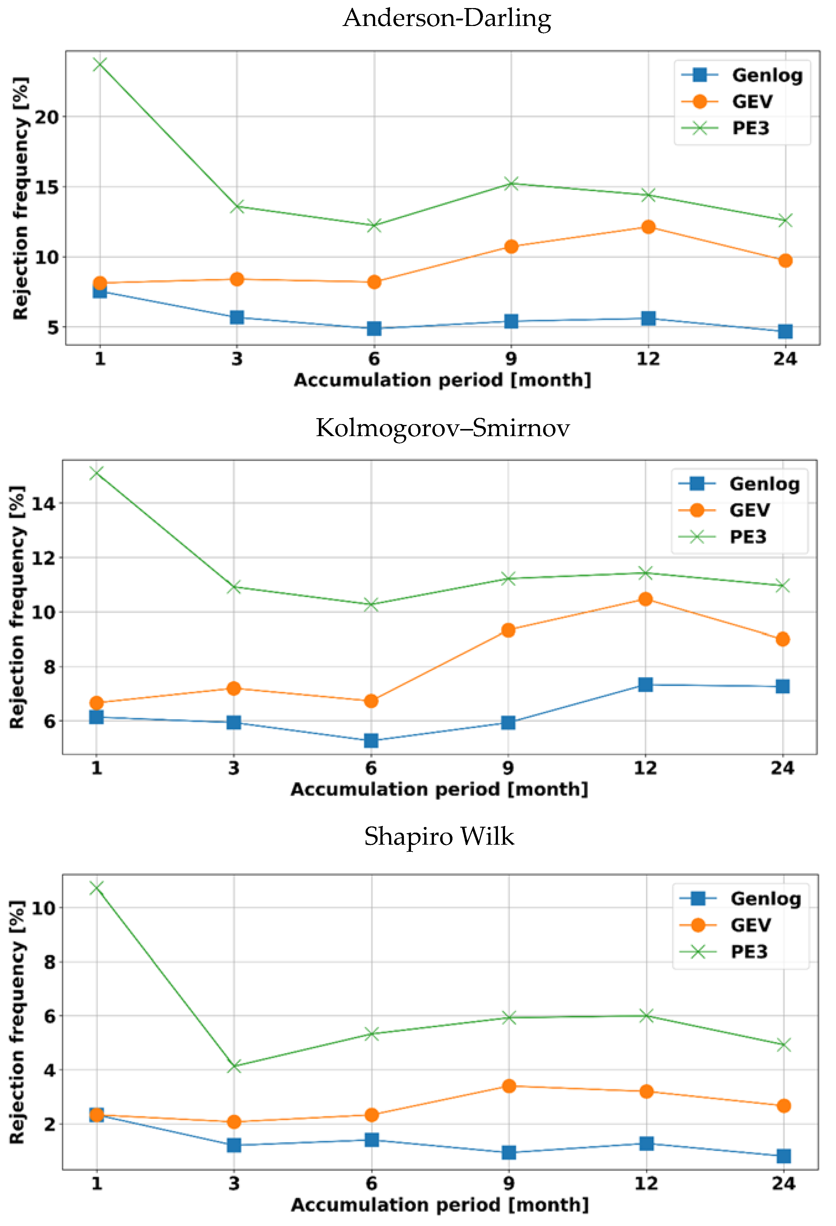
3.2. The Goodness-of-Fit Test

The Genlog distribution captures the water balance better than the other two for all accumulation periods, although comparable results are obtained with the GEV for 1-month accumulation periods. In general, the rejection frequency for Genlog (based on the AD test) is around 5% for most accumulation periods (Figure 2). A similar pattern is seen based on the Kolmogorov–Smirnov (KS) test, but the rejection frequency is lower than for the AD test, which indicates a better fitting in bulk than in the tails of the distribution.

The results for the SW test show a similar pattern to the AD and KS test, except that the rejection frequency is smaller. The ability of the SW test to assess the goodness of fit is essential as it is not required to perform Monte Carlo simulations to find critical values (they are already well known), which is the case for the AD and KS tests [56,57,58].

Similar to our results, higher rejection frequencies at shorter timescales are also seen in Ref. [11] and for the most part of Europe and India [11,12]. The noticeable higher rejection frequency at the 1-month accumulation for the Genlog distribution is further investigated using the quantile–quantile (Q–Q) plot (refer to Figure S3 in Supplementary Material). According to the Q–Q plot, the quantiles deviate from the bisector line for the shorter aggregation level while they approximately lie on the bisector line for a higher timescale.

Furthermore, the acceptance frequency for the GOF test for each month and each accumulation period is provided in Figure S4 in the Supplementary Material. The result indicates that lower acceptance is seen during the 1-month accumulation period. The smallest acceptance percentage is observed in December, January, and February, where the weather is dry in most parts of Ethiopia. However, accumulation periods longer than 3 months show more than 85% acceptance frequency for Genlog. Furthermore, the results are similar to Ref. [13], where the appropriateness of Genlog and the acceptance of the three distributions for SPEI estimation is seen for most parts of China.

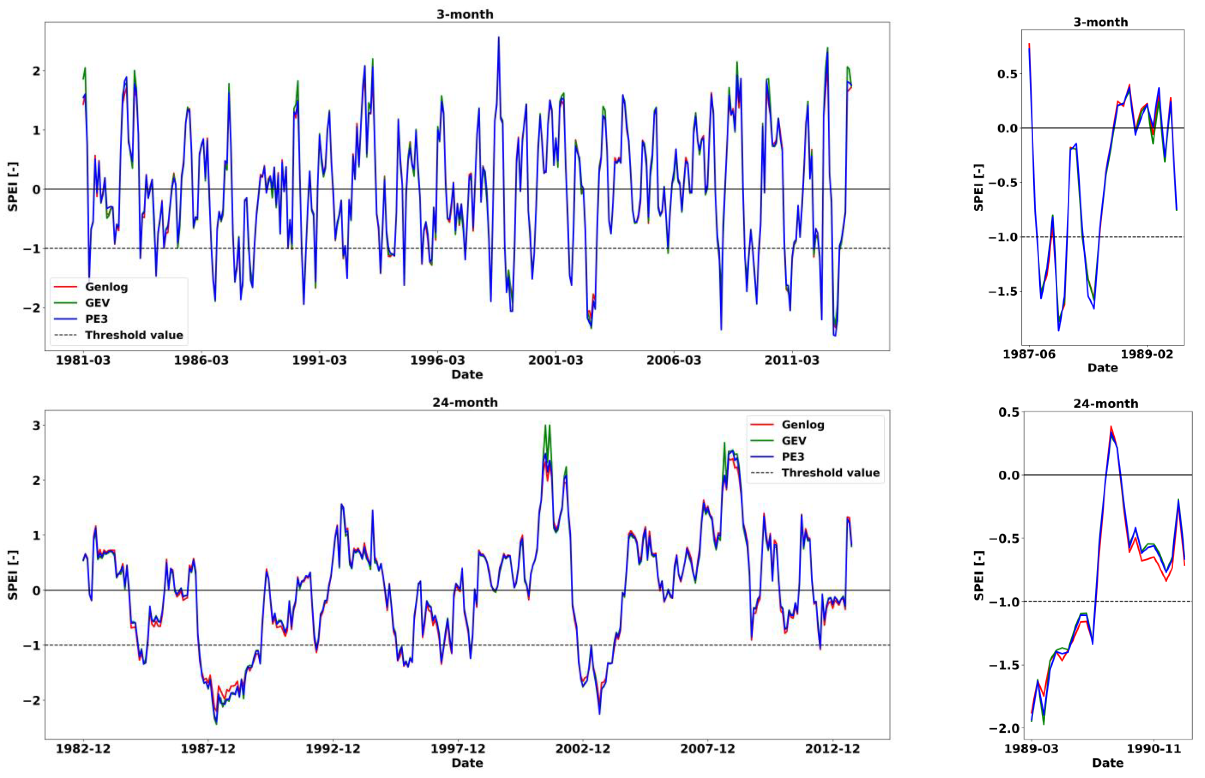
3.3. Comparison of SPEI Values Estimated from PE3, GEV, and Genlog

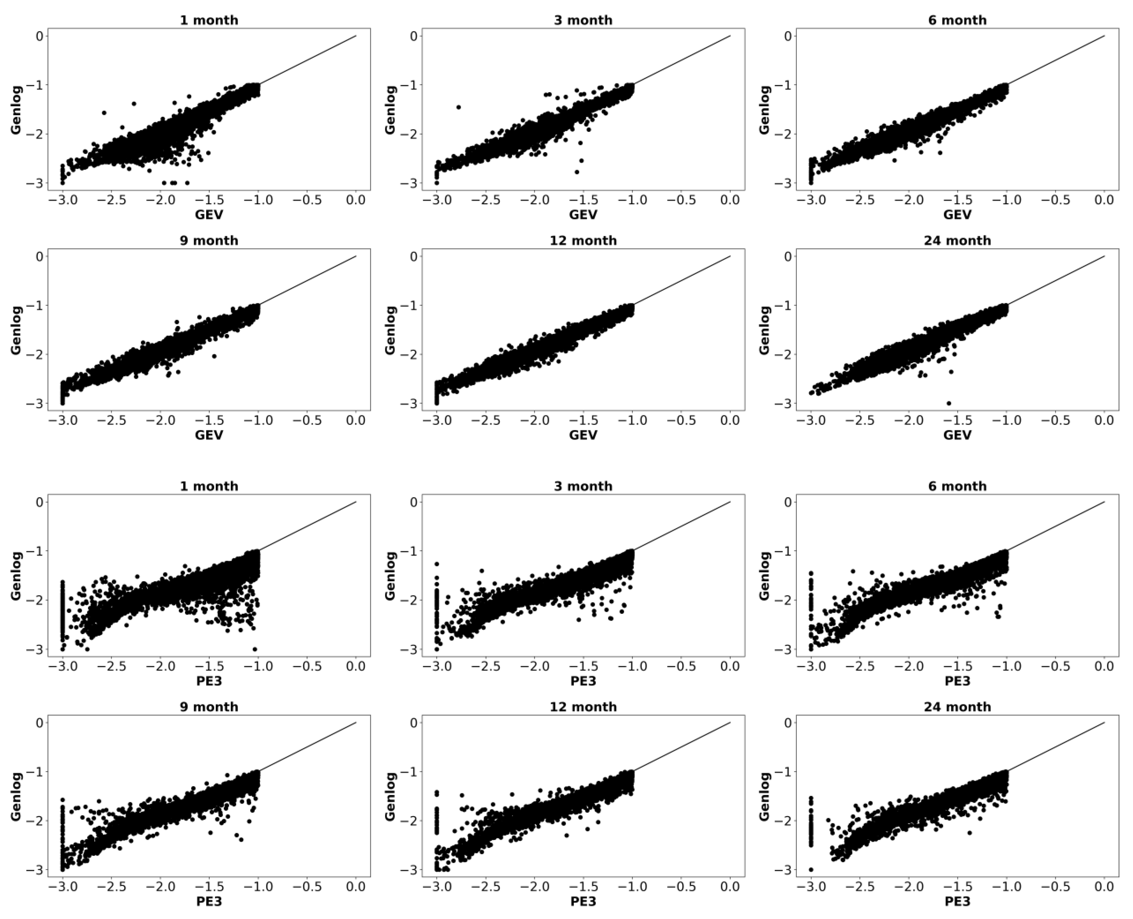
3.3.1. Visual Comparison of SPEI Values

The gauging station (Melkasa) has the lowest number of missing data and is, therefore, used to visually compare the SPEI estimations (Figure S1 of the Supplementary Material). There is a very good overall agreement between all distributions, with an NSE-value around 0.99 (Figure 3). Nevertheless, differences appear for extreme SPEI values, consistent with the aforementioned conclusion that the candidate distributions are a better fit in the bulk of distribution than in the tails. Genlog estimates high severity values of both extreme dry periods (low negative SPEI values) and extremely wet periods (high positive SPEI values) with respect to both the GEV and the PE3 distributions.

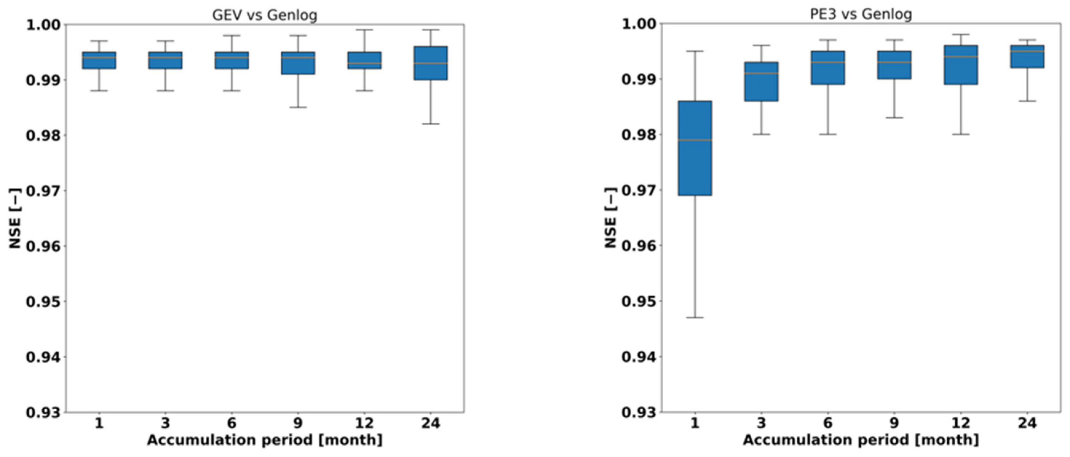
3.3.2. Similarity Analysis Using NSE

Figure 4 shows the NSE values (see Equation (6)) where the Genlog distribution is taken as a reference because it was found in Section 3.2 that it is the most appropriate distribution. The median NSE values consistently exceed 0.97. This implies that the PE3, GEV, and Genlog distributions show a very strong similarity in the bulk of the distribution. The NSE is not very different over the timescales, except the similarity is considerable between the Genlog and the GEV distributions than between the Genlog and the PE3 distributions. The similarity and differences over the distribution functions are also seen spatially in Figure S5 of the Supplementary Material. Moreover, the three probability distribution functions show significant differences mainly at shorter rather than longer time scales. This is also in line with our finding in Figure 2, where differences appear to be higher at the 1-month aggregation level and mostly decrease for the longer accumulation periods. This can be attributed to the difficulty of fitting smaller water balance values, especially for the PE3 distribution, as explored in Section 3.1.

The lowest NSE values are obtained for shorter accumulation periods when comparing the PE3 distribution with the Genlog distribution. Upon comparison of the GEV with the Genlog, median NSE values (from the 125 gauging stations) are relatively independent of the accumulation period. They exceed 0.98, indicating their high degree of similarity, contrary to findings in Ref. [59].

3.3.3. Comparison Based on Drought Events

Assessment is made on how well the different distributions managed to capture drought events since the above analysis with NSE only indicates the performance of the overall distribution. A drought event occurs when SPEI drops below minus one. Hence, SPEI values estimated from PE3, Genlog, or GEV are compared against the selected distribution in a scatter plot (Figure 5). The Genlog is considered to yield the most correct SPEI values; thus, a relative comparison is made by taking SPEI estimated using the Genlog as a reference. The Genlog-based and the GEV-based estimations seem to agree on average for all drought values (Figure 5).

On the contrary, SPEI values from the PE3 are less than and greater than the corresponding SPEI values by the Genlog near −1 (moderate droughts) and near −2 (extreme droughts), respectively. This prevails in most accumulation periods, especially at shorter timescales. The overestimations can be misleading as too frequent drought events can be identified, and their severity can be overestimated.

From all the analyses presented in the previous paragraphs, the differences are considerable, highlighting the importance of proper distribution selection for SPEI-based drought monitoring.

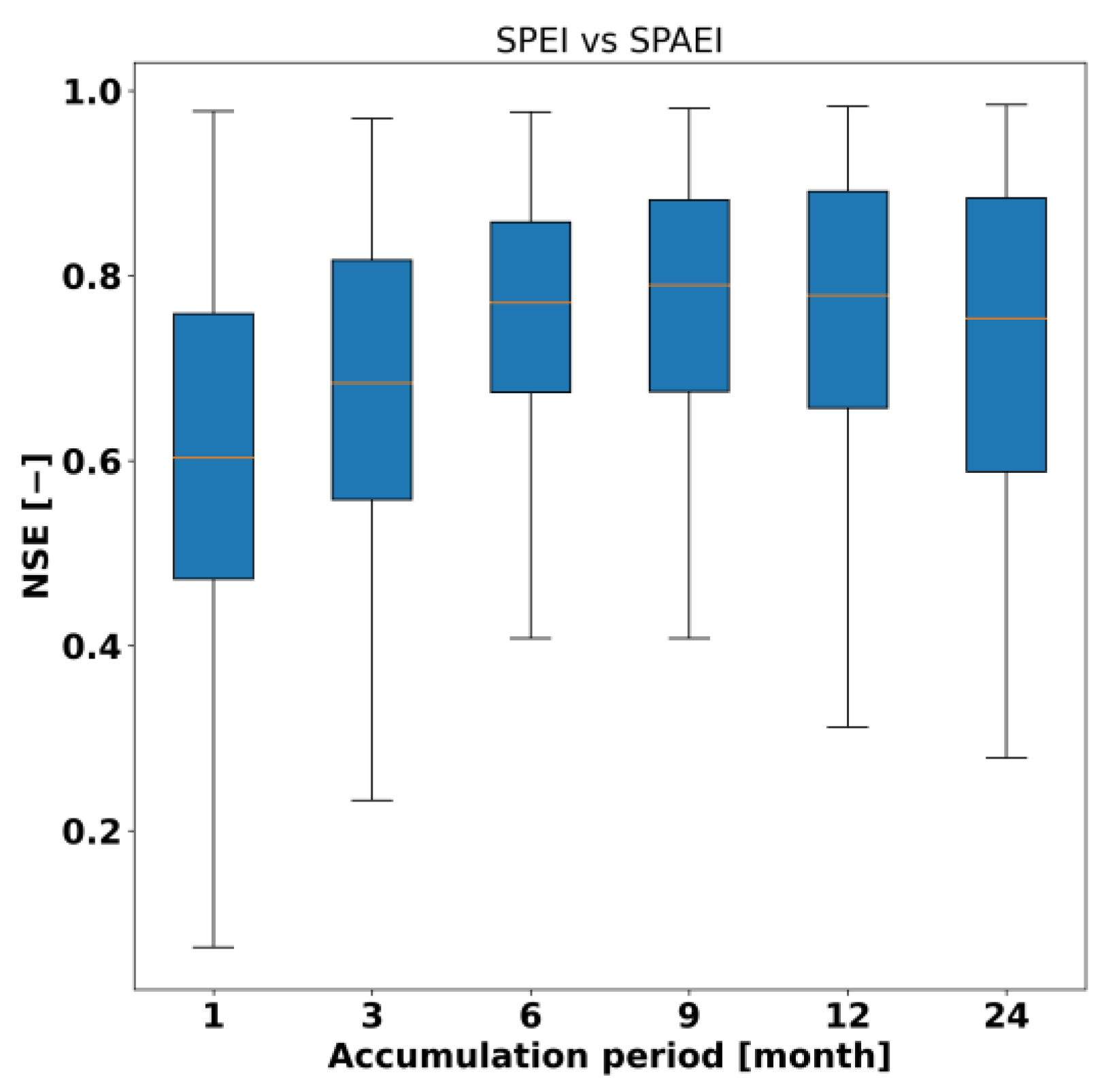
3.4. Standardized Precipitation Actual Evapotranspiration Index (SPAEI)

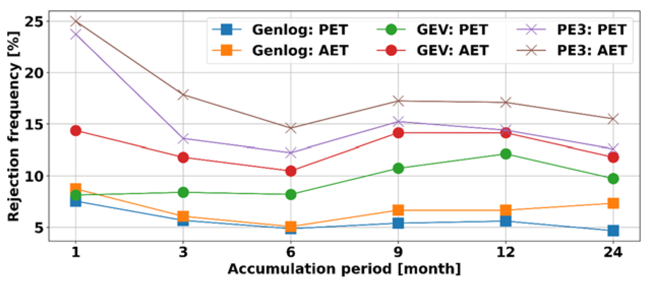
A GOF test is performed using the AD test, and the rejection frequency is calculated (Figure 6). In addition, a comparison of the SPEI and SPAEI values is made using NSE (Equation (6)) to investigate their difference. SPAEI is calculated following the same procedure as SPEI, except that PET is replaced with AET.

3.4.1. GOF Test

The goodness-of-fit for SPAEI shows that the rejection frequency has increased for all cases with respect to SPEI (Figure 6), particularly for the GEV distribution. As was the case for SPEI, Genlog features the lowest rejection frequency and can therefore be considered the appropriate method to fit SPAEI.

3.4.2. Comparison of the SPEI and SPAEI Values

SPEI and SPAEI values are compared in Figure 7 using the NSE score (see Equation (6)), calculated by taking the Genlog-based SPEI values as a reference. The result indicates that there are instances with significant differences (negative NSE values). On the contrary, a maximum NSE value of 1 is also seen, implying that the SPEI values using either AET or PET will not significantly differ in some gauging stations. Only a quarter of the 125 stations shows NSE below 0.5 in all accumulation periods.

The increase of NSE values as a function of the accumulation period indicates a reduced sensitivity to changes in evapotranspiration (ET) for longer accumulation periods. However, additional AET datasets ought to be used to reach a more complete conclusion. Nevertheless, more extended AET datasets were not readily available by the time this research was conducted. In addition, such differences imply that utmost care needs to be given for uncertainty analysis on drought index estimation [30,59,60,61,62].

It is important to note that the PET estimation using the method of Thornthwaite has its limitations, such as overestimation of PET around tropical areas; hence, there is uncertainty in the PET values. The finding of Ref. [63] on the comparison made between the SPEI and SPAEI showed that there is a significant difference between them, which is also seen in our results, which ultimately implies that for Ethiopia, they cannot be assumed equivalent and the drought index should be chosen with care depending on the impact.

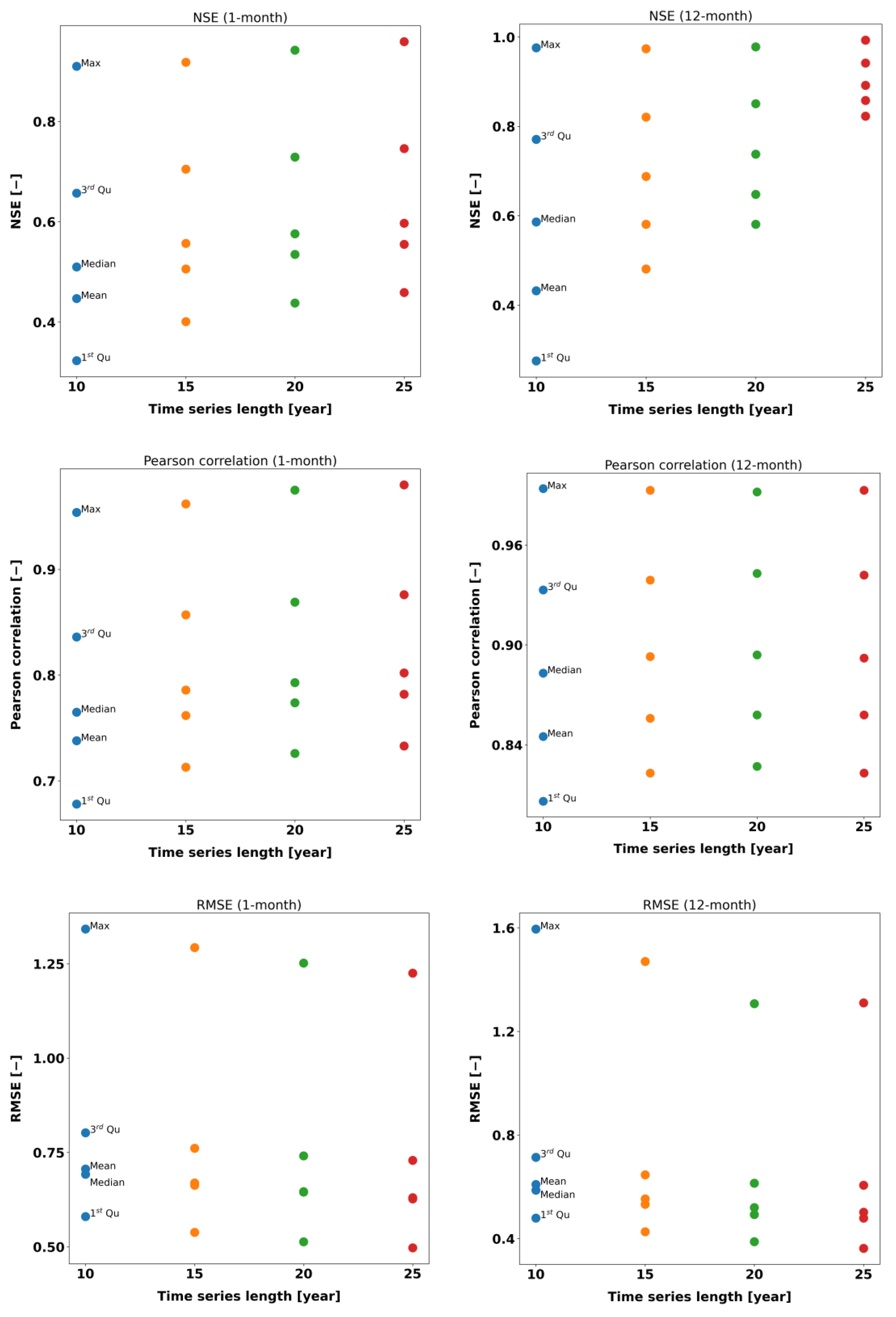
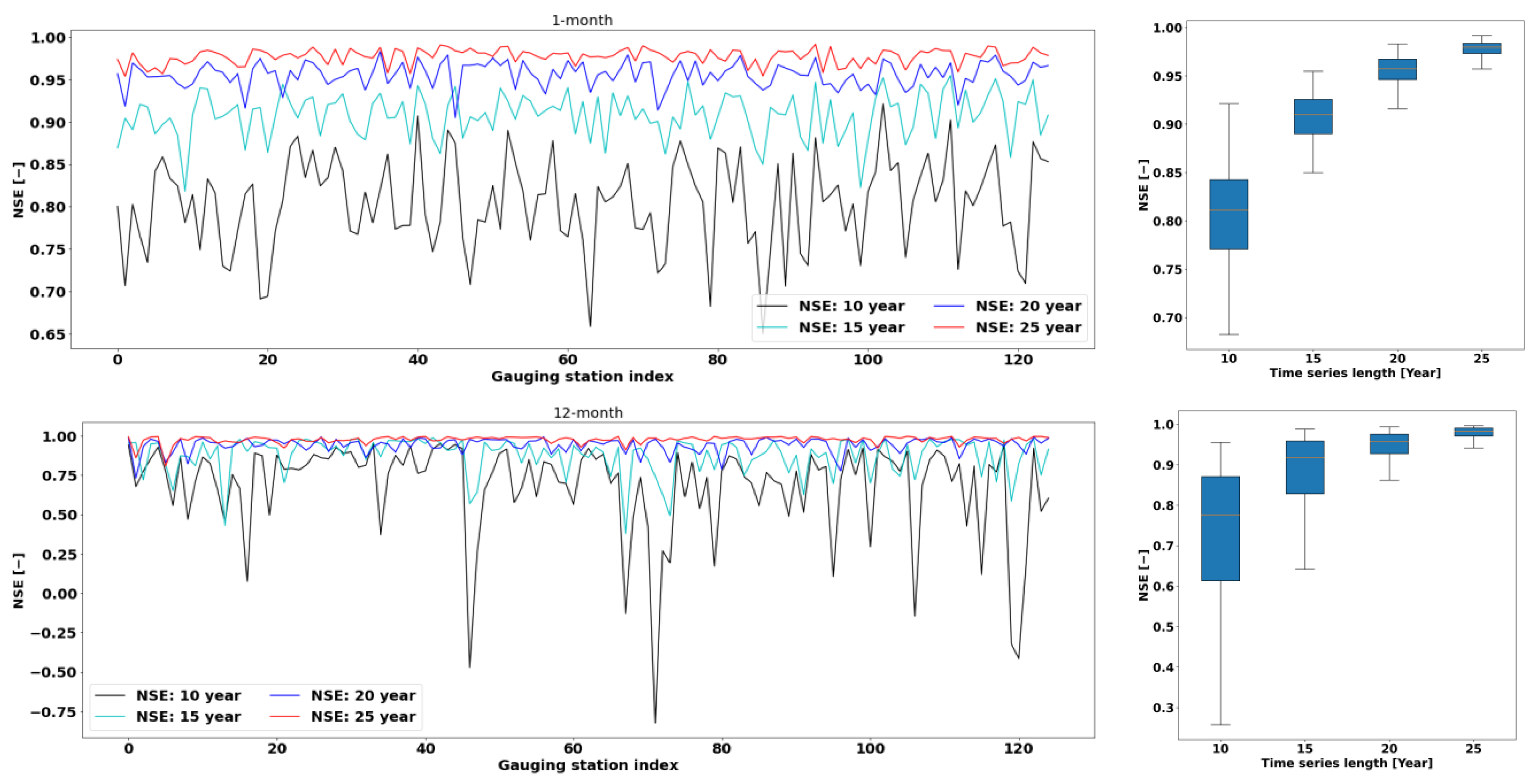
3.5. Shorter Time Series Data Analysis

3.5.1. GOF Test

The AD test results so far suggested that Genlog is the best distribution to fit both the water balance indices SPEI and SPAEI.

Table 1. The AD test rejection frequency (%) for the Genlog distribution for water balance (P-PET) time series data with lengths of 10, 15, 20, and 25 years for all accumulation periods.

		Accumulation Period (Months)
Time Series Length	1	3	6	9	12	24
10	4.04	4.79	5.74	7.27	8.13	12.83
15	3.67	2.48	2.09	2.17	2.16	3.00
20	5.87	4.03	4.05	3.78	4.31	3.61
25	7.13	5.19	4.57	4.43	5.38	5.48

shows the rejection frequency for Genlog-based SPEI for time series lengths of 15, 20, and 25 years. In general, the rejection frequency decreases as the time series length decreases. However, the 10-year data deviate from this trend which can be due to the few data points (only 10) which are used by the distribution function to fit the data.

3.5.2. SPEI Value Comparison between Shorter Length and Benchmark Data

Here evaluation is made to understand the extent to which the lower rejection frequency for shorter time series affects the SPEI values during droughts. In addition, Pearson correlation coefficient and root mean square error (RMSE) are used to compare the SPEI values estimated using 10-, 15-, 20-, and 25-year data against the full time series (above 30 years). Therefore, NSE, RMSE, and Pearson correlation coefficients are calculated, assuming the whole time series data as a reference. The results are shown in Figure 8 and indicate significant differences between 10-year estimations and the benchmark data.

The NSE and Pearson correlation coefficient increase as the time series length increases while the RMSE decreases. For some gauging stations, at shorter/longer accumulation periods, the 10-, 15-, 20-, and 25-year data produce SPEI values significantly different from those estimated using the benchmark data. Following the definition set in Ref. [55], where NSE above 0.4 is satisfactory, our result suggests that only a quarter of the NSE has values less than 0.4 for 15 and above years of time series. Moreover, the statistics indicate that using 20 and 25 years of data will result in almost similar (quartiles of the NSE is almost identical) SPEI values (Figure 8). This indicates the applicability of using shorter-length in situ data to estimate SPEI, compared to the 30 years recommended by the World Meteorological Agency (WMO). Similar results were obtained for SPI estimations using 17 years of data in China [20].

In order to visualize the difference in the SPEI values estimated from the different lengths of time series, Figure 9 shows the NSE calculated based on the SPEI in drought-hit periods (i.e., more historical droughts are recorded) against those estimated using benchmark data (but the comparison is made in the same time window). As expected, the SPEI estimated using 10-year data features the lowest NSE during droughts. NSE values based on 20 and 25 years of data are all higher than 0.9 (1-month accumulation) and 0.7 (12-month accumulation).

4. Conclusions

Different probability distribution functions are tested for estimating SPEI. The Pearson type 3 (PE3), the generalized extreme value (GEV), and the generalized logistic (Genlog) distributions are assessed to statistically model the water balance (precipitation–potential evapotranspiration). The case study is based in Ethiopia, where meteorological data from 125 gauging stations are used. Missing data in the precipitation time series were filled with values from the CHIRPS global dataset. Furthermore, the use of actual evapotranspiration (AET) from the GLEAM dataset instead of potential evapotranspiration (PET) estimated using the method of Thornthwaite was investigated to further assess distribution selection. Finally, the impact of limited data lengths (10, 15, 20, and 25 years) on SPEI estimation was assessed.

First, the Anderson–Darling (AD), Kolmogorov–Smirnov (KS), and Shapiro–Wilk (SW) tests were made to assess the goodness-of-fit of the distribution for the whole dataset (longer than 30 years). It is observed that the rejection frequency for the Genlog is lower than the GEV and the PE3 at a 5% significance level for accumulation periods 1–24 months. Furthermore, for the Genlog, it is seen that the 1-month aggregation level has the highest rejection frequency, and the rejection prevails in the dry months (December, January, and February). Further research is necessary to find an appropriate probability distribution function for 1-month timescales.

The distribution selection has indicated that the Genlog distribution is the most appropriate one, but the difference among the SPEI values estimated from the three distributions can be low (median NSE is above 0.98). Although there is an overall similarity among the SPEI time series, there is a considerable difference in the extreme dry/wet periods for the three distributions.

The use of AET instead of PET to characterize drought can be beneficial to address specific drought impacts, and finding an appropriate distribution function is vital. The use of AET has not changed the distribution selection. However, a significant difference is seen between SPEI and SPAEI, which signifies the necessity to choose appropriate water balance values (based on AET or PET) for drought analysis in Ethiopia.

Finally, the use of shorter time series for SPEI estimation was analyzed, and it was found that the estimation of SPEI is still possible with 15, 20, and 25 years of data. However, there are instances where the SPEI values calculated using shorter length data can be quite different (NSE < 0) from those estimated using the benchmark data (above 30 years data). However, data in most gauging stations with 20 and 25 years of length resulted in similar SPEI values to those estimated from the benchmark data (with NSE up to 1). Hence, 20 and 25 years of data can be used with nearly as equal accuracy as the benchmark data, especially for longer accumulation periods.

References

1. Bayissa, Y.; Maskey, S.; Tadesse, T.; Van Andel, S.J.; Moges, S.; Van Griensven, A.; Solomatine, D. Comparison of the performance of six drought indices in characterizing historical drought for the upper Blue Nile basin, Ethiopia. Geosciences 2018, 8, 81. [Google Scholar] [CrossRef] [Green Version]
2. Wolde-Georgis, T. El Nino and drought early warning in Ethiopia. Internet J. Afr. Stud. 1997. Available online: https://ssrn.com/abstract=1589710 (accessed on 17 May 2021).
3. Viste, E.; Korecha, D.; Sorteberg, A. Recent drought and precipitation tendencies in Ethiopia. Theor. Appl. Climatol. 2013, 112, 535–551. [Google Scholar] [CrossRef] [Green Version]
4. Zeleke, T.T.; Giorgi, F.; Diro, G.T.; Zaitchik, B.F. Trend and periodicity of drought over Ethiopia. Int. J. Climatol. 2017, 37, 4733–4748. [Google Scholar] [CrossRef]
5. Mera, G.A. Drought and its impacts in Ethiopia. Weather Clim. Extrem. 2018, 22, 24–35. [Google Scholar] [CrossRef]
6. Liou, Y.-A.; Mulualem, G.M. Spatio–temporal assessment of drought in ethiopia and the impact of recent intense droughts. Remote Sens. 2019, 11, 1828. [Google Scholar] [CrossRef] [Green Version]
7. McKee, T.B.; Doesken, N.J.; Kleist, J. The relationship of drought frequency and duration to time scales. In Proceedings of the 8th Conference on Applied Climatology, Anaheim, CA, USA, 17–22 January 1993; Volume 17, pp. 179–183. [Google Scholar]
8. Vicente-Serrano, S.M.; Beguería, S.; López-Moreno, J.I. A multiscalar drought index sensitive to global warming: The standardized precipitation evapotranspiration index. J. Clim. 2010, 23, 1696–1718. [Google Scholar] [CrossRef] [Green Version]
9. Van de Vyver, H.; Van den Bergh, J. The Gaussian copula model for the joint deficit index for droughts. J. Hydrol. 2018, 561, 987–999. [Google Scholar] [CrossRef]
10. da Rocha Júnior, R.L.; dos Santos Silva, F.D.; Costa, R.L.; Gomes, H.B.; Pinto, D.D.C.; Herdies, D.L. Bivariate assessment of drought return periods and frequency in brazilian northeast using joint distribution by copula method. Geosciences 2020, 10, 135. [Google Scholar] [CrossRef] [Green Version]
11. Stagge, J.H.; Tallaksen, L.M.; Gudmundsson, L.; Van Loon, A.F.; Stahl, K. Candidate distributions for climatological drought indices (SPI and SPEI). Int. J. Climatol. 2015, 35, 4027–4040. [Google Scholar] [CrossRef]
12. Monish, N.T.; Rehana, S. Suitability of distributions for standard precipitation and evapotranspiration index over meteorologically homogeneous zones of India. J. Earth Syst. Sci. 2020, 129, 25. [Google Scholar] [CrossRef]
13. Wang, H.; Chen, Y.; Pan, Y.; Chen, Z.; Ren, Z. Assessment of candidate distributions for SPI/SPEI and sensitivity of drought to climatic variables in China. Int. J. Climatol. 2019, 39, 4392–4412. [Google Scholar] [CrossRef]
14. García-Valdecasas Ojeda, M.; Yeste Donaire, P.; Góngora García, T.M.; Raquel Gámiz-Fortis, S.; Castro-Díez, Y.; Jesús Esteban-Parra, M. Evaluating the Feasibility of Using a Drought Index Based on the Actual Evapotranspiration. In Proceedings of the EGU General Assembly Conference Abstracts, Vienna, Austria, 8–13 April 2018; p. 15169. [Google Scholar]
15. Rehana, S.; Naidu, G.S. Development of hydro-meteorological drought index under climate change–Semi-arid river basin of Peninsular India. J. Hydrol. 2021, 594, 125973. [Google Scholar] [CrossRef]
16. Zhang, G.; Gan, T.Y.; Su, X. Twenty-first century drought analysis across China under climate change. Clim. Dyn. 2021, 1–21. [Google Scholar] [CrossRef]
17. Rehana, S.; Monish, N.T. Characterization of regional drought over water and energy limited zones of India using potential and actual evapotranspiration. Earth Space Sci. 2020, 7, e2020EA001264. [Google Scholar] [CrossRef]
18. Faiz, M.A.; Liu, D.; Fu, Q.; Naz, F.; Hristova, N.; Li, T.; Niaz, M.A.; Khan, Y.N. Assessment of dryness conditions according to transitional ecosystem patterns in an extremely cold region of China. J. Clean. Prod. 2020, 255, 120348. [Google Scholar] [CrossRef]
19. Bayissa, Y.A.; Moges, S.A.; Xuan, Y.; Van Andel, S.J.; Maskey, S.; Solomatine, D.P.; Griensven, A.V.; Tadesse, T. Spatio-temporal assessment of meteorological drought under the influence of varying record length: The case of Upper Blue Nile Basin, Ethiopia. Hydrol. Sci. J. 2015, 60, 1927–1942. [Google Scholar] [CrossRef]
20. Lu, J.; Jia, L.; Menenti, M.; Yan, Y.; Zheng, C.; Zhou, J. Performance of the standardized precipitation index based on the TMPA and CMORPH precipitation products for drought monitoring in China. IEEE J. Sel. Top. Appl. Earth Obs. Remote Sens. 2018, 11, 1387–1396. [Google Scholar] [CrossRef]
21. Van den Hende, C.; Van Schaeybroeck, B.; Nyssen, J.; Van Vooren, S.; Van Ginderachter, M.; Termonia, P. Analysis of rain-shadows in the Ethiopian Mountains using climatological model data. Clim. Dyn. 2021, 56, 1663–1679. [Google Scholar] [CrossRef]
22. Seleshi, Y.; Demarée, G. Identifying the major cause of the prevailing summer rainfall deficit over the North-Central Ethiopian highlands since the mid-60s. In Proceedings of the International Conference on Tropical Climatology, Meteorology and Hydrology in Memoriam Franz Bultot, Bruxelles, Belgium, 22–24 May 1996; Royal Meteorological Institute of Belgium (Brussels); Royal Academy of Overseas Sciences (Brussels): Brussels, Belgium, 1998. [Google Scholar]
23. Seleshi, Y.; Demaree, G. The temporal distribution of Ethiopian meteorological droughts in the 20 century. In Proceedings of the Biological Indicators of Global Change, Brussels, Belgium, 7–9 May 1992. [Google Scholar]
24. Seleshi, Y.; Camberlin, P. Recent changes in dry spell and extreme rainfall events in Ethiopia. Theor. Appl. Climatol. 2006, 83, 181–191. [Google Scholar] [CrossRef] [Green Version]
25. Jury, M.R.; Funk, C. Climatic trends over Ethiopia: Regional signals and drivers. Int. J. Climatol. 2013, 33, 1924–1935. [Google Scholar] [CrossRef]
26. Dosio, A.; Jones, R.G.; Jack, C.; Lennard, C.; Nikulin, G.; Hewitson, B. What can we know about future precipitation in Africa? Robustness, significance and added value of projections from a large ensemble of regional climate models. Clim. Dyn. 2019, 53, 5833–5858. [Google Scholar] [CrossRef] [Green Version]
27. Keller, E.J. Drought, war, and the politics of famine in Ethiopia and Eritrea. J. Mod. Afr. Stud. 1992, 30, 609–624. [Google Scholar] [CrossRef]
28. Funk, C.; Peterson, P.; Landsfeld, M.; Pedreros, D.; Verdin, J.; Shukla, S.; Husak, G.; Rowland, J.; Harrison, L.; Hoell, A. The climate hazards infrared precipitation with stations—A new environmental record for monitoring extremes. Sci. Data 2015, 2, 150066. [Google Scholar] [CrossRef] [PubMed] [Green Version]
29. Bayissa, Y.; Tadesse, T.; Demisse, G.; Shiferaw, A. Evaluation of satellite-based rainfall estimates and application to monitor meteorological drought for the Upper Blue Nile Basin, Ethiopia. Remote Sens. 2017, 9, 669. [Google Scholar] [CrossRef] [Green Version]
30. Dinku, T.; Funk, C.; Peterson, P.; Maidment, R.; Tadesse, T.; Gadain, H.; Ceccato, P. Validation of the CHIRPS satellite rainfall estimates over eastern Africa. Q. J. R. Meteorol. Soc. 2018, 144, 292–312. [Google Scholar] [CrossRef] [Green Version]
31. Hersbach, H.; Bell, B.; Berrisford, P.; Hirahara, S.; Horányi, A.; Muñoz-Sabater, J.; Nicolas, J.; Peubey, C.; Radu, R.; Schepers, D. The ERA5 global reanalysis. Q. J. R. Meteorol. Soc. 2020, 146, 1999–2049. [Google Scholar] [CrossRef]
32. Gleixner, S.; Demissie, T.; Diro, G.T. Did ERA5 improve temperature and precipitation reanalysis over East Africa? Atmosphere 2020, 11, 996. [Google Scholar] [CrossRef]
33. Penman, H.L. Natural evaporation from open water, bare soil and grass. Proc. R. Soc. Lond. Ser. A Math. Phys. Sci. 1948, 193, 120–145. [Google Scholar] [CrossRef] [Green Version]
34. Thornthwaite, C.W. An approach toward a rational classification of climate. Geogr. Rev. 1948, 38, 55–94. [Google Scholar] [CrossRef]
35. Van der Schrier, G.; Jones, P.D.; Briffa, K.R. The sensitivity of the PDSI to the Thornthwaite and Penman-Monteith parameterizations for potential evapotranspiration. J. Geophys. Res. Atmos. 2011, 116, D03106. [Google Scholar] [CrossRef]
36. Stagge, J.H.; Tallaksen, L.M.; Xu, C.Y.; Van Lanen, H.A. Standardized precipitation-evapotranspiration index (SPEI): Sensitivity to potential evapotranspiration model and parameters. In Proceedings of the Hydrology in a Changing World, Montpellier, France, 7–10 October 2014; Volume 363, pp. 367–373. [Google Scholar]
37. Guttman, N.B. Accepting the standardized precipitation index: A calculation algorithm 1. JAWRA J. Am. Water Resour. Assoc. 1999, 35, 311–322. [Google Scholar] [CrossRef]
38. Gudmundsson, L.; Stagge, J.H. SCI: Standardized Climate Indices such as SPI, SRI or SPEI, R Package Version 1.0.1. 2014. Available online: https://rdrr.io/cran/SCI/ (accessed on 17 May 2021).
39. Miralles, D.G.; Holmes, T.R.H.; De Jeu, R.A.M.; Gash, J.H.; Meesters, A.; Dolman, A.J. Global land-surface evaporation estimated from satellite-based observations. Hydrol. Earth Syst. Sci. Discuss. 2010, 7, 8479–8519. [Google Scholar] [CrossRef] [Green Version]
40. Martens, B.; Miralles, D.G.; Lievens, H.; Van Der Schalie, R.; De Jeu, R.A.; Fernández-Prieto, D.; Beck, H.E.; Dorigo, W.A.; Verhoest, N.E. GLEAM v3: Satellite-based land evaporation and root-zone soil moisture. Geosci. Model Dev. 2017, 10, 1903–1925. [Google Scholar] [CrossRef] [Green Version]
41. Peng, J.; Dadson, S.; Hirpa, F.; Dyer, E.; Lees, T.; Miralles, D.G.; Vicente-Serrano, S.M.; Funk, C. A pan-African high-resolution drought index dataset. Earth Syst. Sci. Data 2020, 12, 753–769. [Google Scholar] [CrossRef] [Green Version]
42. Singh, V.P. Pearson type III distribution. In Entropy-Based Parameter Estimation in Hydrology; Springer: Dordrecht, The Netherlands, 1998; pp. 231–251. [Google Scholar]
43. Hosking, J.R. Algorithm as 215: Maximum-likelihood estimation of the parameters of the generalized extreme-value distribution. J. R. Stat. Soc. Ser. C Appl. Stat. 1985, 34, 301–310. [Google Scholar] [CrossRef]
44. Hosking, J.R.M.; Wallis, J.R.; Wood, E.F. Estimation of the generalized extreme-value distribution by the method of probability-weighted moments. Technometrics 1985, 27, 251–261. [Google Scholar] [CrossRef]
45. Gupta, R.D.; Kundu, D. Generalized logistic distributions. J. Appl. Stat. Sci. 2010, 18, 51. [Google Scholar]
46. Massey Jr, F.J. The Kolmogorov-Smirnov test for goodness of fit. J. Am. Stat. Assoc. 1951, 46, 68–78. [Google Scholar] [CrossRef]
47. Anderson, T.W.; Darling, D.A. A test of goodness of fit. J. Am. Stat. Assoc. 1954, 49, 765–769. [Google Scholar] [CrossRef]
48. Chowdhury, J.U.; Stedinger, J.R.; Lu, L.-H. Goodness-of-fit tests for regional generalized extreme value flood distributions. Water Resour. Res. 1991, 27, 1765–1776. [Google Scholar] [CrossRef]
49. Shin, H.; Jung, Y.; Jeong, C.; Heo, J.-H. Assessment of modified Anderson–Darling test statistics for the generalized extreme value and generalized logistic distributions. Stoch. Environ. Res. Risk Assess. 2012, 26, 105–114. [Google Scholar] [CrossRef]
50. Song, S.; Singh, V.P. Meta-elliptical copulas for drought frequency analysis of periodic hydrologic data. Stoch. Environ. Res. Risk Assess. 2010, 24, 425–444. [Google Scholar] [CrossRef]
51. Delignette-Muller, M.L.; Pouillot, R.; Denis, J.-B.; Dutang, C. Fitdistrplus: Help to Fit of a Parametric Distribution to Non-Censored or Censored Data, 2010; R Package Version 01-3. 2013. Available online: https://cran.r-project.org/web/packages/fitdistrplus/fitdistrplus.pdf (accessed on 17 May 2021).
52. Asquith, W. Package ‘Lmomco.’ L-Moments, Trimmed L-Moments, L-Comoments, and Many. 2021. Available online: https://cran.r-project.org/web/packages/lmomco/lmomco.pdf (accessed on 17 May 2021).
53. Shapiro, S.S.; Wilk, M.B. An analysis of variance test for normality (complete samples). Biometrika 1965, 52, 591–611. [Google Scholar] [CrossRef]
54. Nash, J.E.; Sutcliffe, J.V. River flow forecasting through conceptual models part I—A discussion of principles. J. Hydrol. 1970, 10, 282–290. [Google Scholar] [CrossRef]
55. Xia, Y.; Ek, M.B.; Peters-Lidard, C.D.; Mocko, D.; Svoboda, M.; Sheffield, J.; Wood, E.F. Application of USDM statistics in NLDAS-2: Optimal blended NLDAS drought index over the continental United States. J. Geophys. Res. Atmos. 2014, 119, 2947–2965. [Google Scholar] [CrossRef]
56. Lilliefors, H.W. On the Kolmogorov-Smirnov test for normality with mean and variance unknown. J. Am. Stat. Assoc. 1967, 62, 399–402. [Google Scholar] [CrossRef]
57. Crutcher, H.L. A note on the possible misuse of the Kolmogorov-Smirnov test. J. Appl. Meteorol. 1975, 14, 1600–1603. [Google Scholar] [CrossRef] [Green Version]
58. Steinskog, D.J.; Tjøstheim, D.B.; Kvamstø, N.G. A cautionary note on the use of the Kolmogorov–Smirnov test for normality. Mon. Weather Rev. 2007, 135, 1151–1157. [Google Scholar] [CrossRef]
59. Zhang, Y.; Li, Z. Uncertainty analysis of Standardized Precipitation Index due to the effects of probability distributions and parameter errors. Front. Earth Sci. 2020, 8, 76. [Google Scholar] [CrossRef]
60. Burke, E.J.; Brown, S.J. Evaluating uncertainties in the projection of future drought. J. Hydrometeorol. 2008, 9, 292–299. [Google Scholar] [CrossRef]
61. Hoffmann, D.; Gallant, A.J.; Arblaster, J.M. Uncertainties in drought from index and data selection. J. Geophys. Res. Atmos. 2020, 125, e2019JD031946. [Google Scholar] [CrossRef]
62. Xu, K.; Wu, C.; Zhang, C.; Hu, B.X. Uncertainty assessment of drought characteristics projections in humid subtropical basins in China based on multiple CMIP5 models and different index definitions. J. Hydrol. 2021, 600, 126502. [Google Scholar] [CrossRef]
63. Homdee, T.; Pongput, K.; Kanae, S. A comparative performance analysis of three standardized climatic drought indices in the Chi River basin, Thailand. Agric. Nat. Resour. 2016, 50, 211–219. [Google Scholar] [CrossRef] [Green Version]
Figure 1. Elevation map for the study area together with the location of the 125 gauging stations used in this study.
Atmosphere 13 00364 g001
Figure 2. Rejection frequency (relative to 125 stations and 12 months per station) for the Anderson–Darling (top), Kolmogorov–Smirnov (middle), and Shapiro–Wilk (bottom) goodness-of-fit test at 5% significance level. The result is for the three SPEI candidate distribution functions for different accumulation timescales.
Atmosphere 13 00364 g002
Figure 3. Comparison between the SPEI time series estimated based on the PE3, GEV, and Genlog distributions for 3 and 24 accumulation periods at Melkasa (IAR) gauging station. Zoomed-in plot is given on the side for both 3- and 24-month aggregation levels.
Atmosphere 13 00364 g003
Figure 4. Boxplots of the NSE values (see Equation (6)) of 125 gauging station SPEI values at different accumulation periods when the GEV and the PE3 distribution are compared relative to the Genlog distribution (left and right, respectively).
Atmosphere 13 00364 g004
Figure 5. Scatter plot of the SPEI values estimated using all 125 gauging stations for all the accumulation periods whose values are less than −1 where both the PE3 and the GEV distribution are compared relative to the Genlog distribution.
Atmosphere 13 00364 g005
Figure 6. The AD goodness-of-fit test results for SPAEI (labeled orange, red, and brown lines) compared to SPEI (labeled blue, green, and purple).
Atmosphere 13 00364 g006
Figure 7. Comparison between SPEI and SPAEI with the NSE score (see Equation (6)). The rows indicate the mean, minimum, quartiles, and maximum NSE values of the different stations for each accumulation period (columns).
Atmosphere 13 00364 g007
Figure 8. Comparison made between SPEI estimated using shorter and above 30 years of water balance data. Shown are the first quartile (1st Qu.), median, mean, third quartile (3rd Qu.), and maximum (Max.) of the NSE, Pearson correlation (Pearson cor.), and root mean square error (RMSE) for 1- and 12-month timescales for 10-, 15-, 20- and 25-year-long time series data.
Atmosphere 13 00364 g008
Figure 9. The variation of the NSE among 10-, 15-, 20-, and 25-year water balance data for 1-month and 12-month accumulation periods. In addition, boxplots on the side are presented to summarize the NSE from the 125 gauging stations. This is based on 10, 15, 20, and 25 years of data selected by looking at the most drought-hit period.
Atmosphere 13 00364 g009