1. Introduction
Ozone (O
3) is an important component of the atmosphere, most of which lies in the stratosphere, and a small part exists in the troposphere. Stratospheric O
3 can protect terrestrial organisms from radiation hazards by absorbing external ultraviolet radiation. As a greenhouse gas, O
3 can absorb solar radiation reflected from the ground and re-emit the radiation, hence contributing to global warming and climatic change [
1]. The precursors of tropospheric O
3 are generally nitrogen oxides (NO
x) and volatile organic compounds (VOC
s) [
2]. The reaction process is as follows:
The formation process of O
3 is extremely nonlinear [
3]. The increase of O
3 concentrations in the troposphere can potentially affect the health of human beings, animals and plants. In a high-concentration O
3 environment, human beings are prone to respiratory diseases and the growth and output of crops are inhibited [
4]. In Beijing, China, control experiments in an open-top chamber (OTC) with different O
3 concentrations showed that with increasing O
3 concentrations, the biomass of trees decreased significantly, the net photosynthetic rate and transpiration rate decreased, the intercellular carbon dioxide concentration increased and the chlorophyll content, stomatal area and stomatal opening were also affected [
5]. Leaves became sapless, yellow, even died. In addition, the root biomass, fine root yield, turnover and underground carbon availability of trees decreased [
6]. Hence high O
3 concentrations can cause agricultural and forestry industries to reduce their production and reduce their economic outputs.
Monitoring O
3 concentration is an important task for controlling air pollution [
7]. The composition of the atmosphere is influenced by the development of industrialization and urbanization and the enhancement of human activities. The atmospheric content of sulfur dioxide (SO
2), nitrogen oxides (NO
x), ozone (O
3), respirable particulate matter (PM
10) and respirable particulate matter (PM
2.5) are constantly increasing. Air pollution has become a serious problem endangering human health and the survival of animals and plants.
In recent years, human activities have greatly increased the O
3 precursors discharged into the atmosphere, creating conditions for increasing O
3 concentrations. Pollution caused by O
3 is serious in urban areas, especially in the Beijing-Tianjin-Hebei, Yangtze River Delta and Pearl River Delta urban agglomerations in China [
8,
9,
10]. In 2019, PM
2.5, PM
10, SO
2, NO
2 and CO in 338 prefecture-level cities all declined in part, while only O
3 concentration increased by 6.5% year-on-year [
11]. Restrictions on nitrogen oxides emissions have achieved remarkable results, but VOCs have been increasing. Many countries in the world actively respond to O
3 pollution. They have shown that single control of volatile organic compounds (VOCs), coordinated control of VOCs and NOx, local controls and regional coordinated prevention initiatives can all achieve remarkable results [
12]. However, at present, China mainly adopts comprehensive control measures, such as monitoring, early warning and limiting the discharge of precursors [
13].
Previous studies have shown that there are daily and weekly cycles of ozone and local ozone concentrations can be influenced by upwind transport [
14], weekly cycles of VOCs/NOx and aerosol concentrations [
15], as well as the surrounding environment [
16,
17]. Furthermore, the seasonal cycle of O
3 is significant [
18,
19]. Changes in ozone precursor emissions [
20], synoptic weather [
21], summer monsoon and farmland biomass burning [
22] have all been shown to influence the seasonal cycle of ozone. Research conducted in southern California [
23], Los Angeles [
24], New York [
25] and their surrounding areas [
26] have demonstrated the weekly cycle of urban O
3. On a daily timescale, O
3 usually presents a unimodal characteristic [
27], and some studies have used the daily cycle as the standard against which to test the simulation effect of O
3 models.
The main factors affecting the spatial distribution characteristics of O
3 include the presence of precursors in different regions, differences in photochemical reaction conditions and transport from adjacent sources. For example, Haiying found that there are two O
3 pollution zones in Beijing, one mainly concentrated in Beijing-Baoding-northwestern Shanxi, and the other in Beijing-Tianjin-Bohai [
28]. In recent years, research has focused on the distribution of PM
2.5, PM
10 and NO
2, although the natural and anthropogenic environmental conditions within cities will also determine the spatial characteristics of air pollution [
29].
The variation in O3 concentrations and distribution is of great significance to urban ecological planning and environmental governance. In 2020, the concentration of ozone in Beijing exceeded the national secondary standard by 9.0%, while other pollutants (SO2, NO2, PM10 and PM2.5) were all found to be decreasing. Beijing, as the capital of China, is the pioneer area demonstrating ecological urban planning and governance. Hence, it is urgent to control air pollution in the city and improve the quality of the environment. In order to achieve this, a systematic study of the temporal variation and spatial distribution of ozone pollution in Beijing is needed, as well as an investigation of the relationship between O3 spatial-temporal patterns, climatic conditions and other pollutants in Beijing.
This study uses hourly O3 concentration data from 35 atmospheric monitoring stations within Beijing in 2020 to investigate the temporal and spatial distribution of O3. Meteorological data is used to explore the relationship between ozone concentrations and meteorological conditions and to investigate the critical factors that affect local air quality. The purpose is to better understand the factors influencing O3 pollution in Beijing in order to provide evidence for the formulation of improved pollution-control policies.
2. Materials and Methods
2.1. The Research Area
Beijing (115.7–117.4° E, 39.4–41.6° N) is located in the northwest of the North China Plain and is surrounded by mountains on three sides, making it difficult for polluted gases to naturally diffuse. The altitude of the Beijing Plain is 20–60 m, and the altitude of the surrounding mountainous areas is generally 1000–1500 m. The regional climate belongs to the warm temperate zone, with four distinct seasons: long winters and summers, short springs and autumns. There is moderate precipitation, long frost-free periods and the annual average temperature is 8–12 °C. The annual average precipitation is about 600 mm, and the seasonal distribution of precipitation is very uneven. A total of 70% of the annual rainfall is concentrated in July, August and September. Forest coverage is about 43.5% in Beijing by area and about 28.5% on the North China Plain. The urban greening areal coverage is about 48.4%.
2.2. Data Sources and Analysis
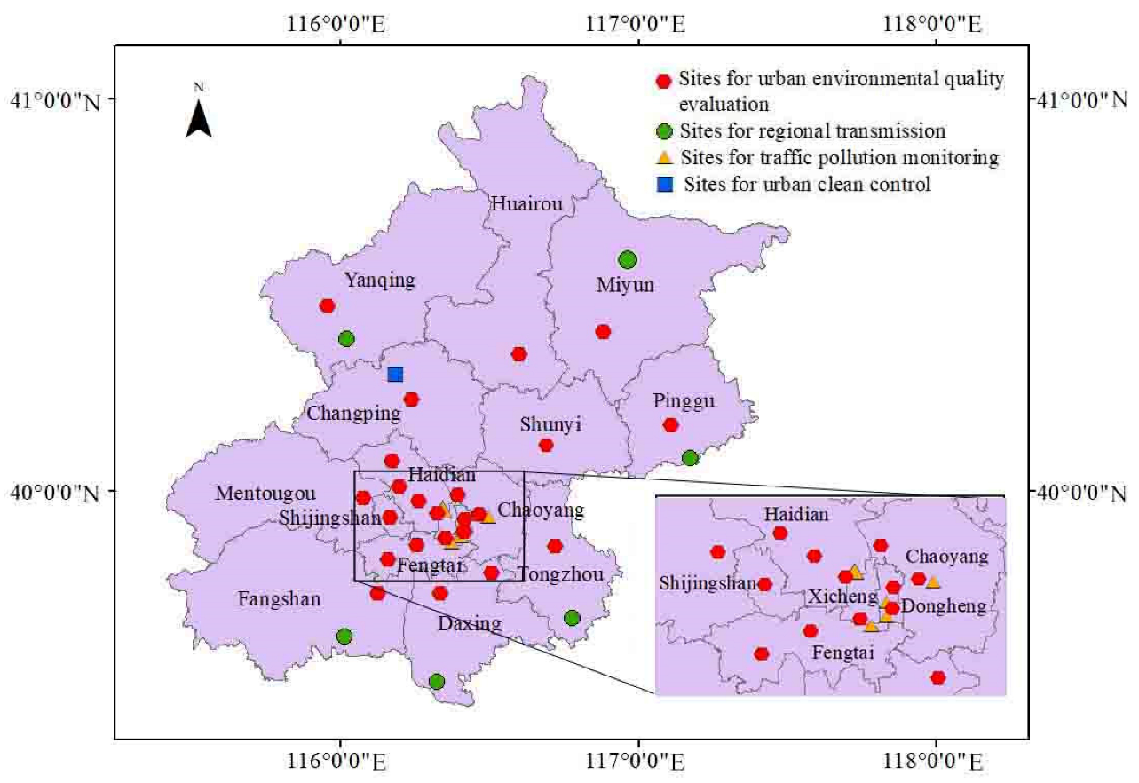
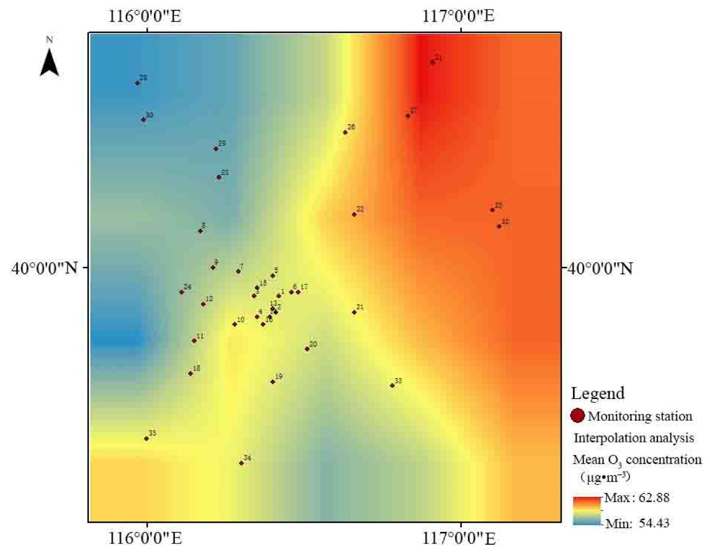
Ozone monitoring data came from 35 monitoring points operated by the Beijing Environmental Protection Monitoring Center (
Figure 1). The sites were categorized as follows: 23 urban environmental assessment sites; 6 regional transmission sites; 5 traffic pollution monitoring sites; and 1 urban clean control site. By geographical location, they were divided between six central districts (17 sites), the northwest of the city center (4 sites), the southwest (3 sites), the northeast (6 sites) and the southeast (5 sites). The data collection period was from January to December 2020.
O3 was monitored using 49C ultraviolet O3 analyzers produced by Thermo Fisher (an American thermoelectric environmental instrument company). The lowest detection limit of the O3 analyzer was 1 ppb, the accuracy was ±1 ppb, the zero drift was 0.4%/24 h and the span drift was 1%/24 h and 2%/7 d.
NO2 concentration was monitored using Thermo Fisher 42C chemiluminescence NO-NO2-NOx analyzers. The lowest detection limit of this analyzer was 0.05 ppb, the zero drift was less than 0.025 × 10⁻⁹/24 h and the span drift was 1%/24 h.
CO concentration was measured using Thermo Fisher 48C analyzers based on the gas filtering infrared absorption method. SO2 was monitored using T E-43C analyzers, employing the ultraviolet fluorescence method.
Meteorological data came from the Beijing meteorological station (No. 54511) and included precipitation, sunshine hours, wind speed, wind direction and maximum/minimum temperature data.
In this study, hourly data of O3 concentration were selected for analysis, and classified on seasonal (monthly), daily and weekly time scales. Spatial analysis was carried out using the geographical categories of urban areas, northeast, northwest, southeast and southwest areas and 16 administrative central areas.
Kriging is an advanced geostatistical procedure that generates an estimated surface from a scattered set of points with values. Kriging methods were used to generate O3 distribution maps based on the monitoring data. Data processing, Kriging interpolation analysis of O3 concentrations and Pearson correlation analysis were carried out using Excel 2010, Arc GIS and SPSS software, respectively.
3. Results
3.1. Temporal Variation
The annual average value of O
3 concentration in Beijing was 59.58 μg·m
−3, and the annual average daily maximum 8 h average concentration was 93.59 μg·m
−3 although this demonstrated significant seasonal variation. With reference to the China Ambient Air Quality Standard (GB 3095—2012) [
30], in 2020, the daily maximum 8 h average O
3 concentration exceeded the primary standard (100 μg·m
−3) for 129 days and the secondary standard (160 μg·m
−3) for 48 days. The highest daily maximum 8 h average in 2020 was 271.91 μg·m
−3. The hourly average O
3 concentration exceeded the primary standard (160 μg·m
−3) for 408 h and the secondary standard (200 μg·m
−3) for 103 h. The highest 2020 value of the hourly average O
3 concentration was 297.03 μg·m
−3.
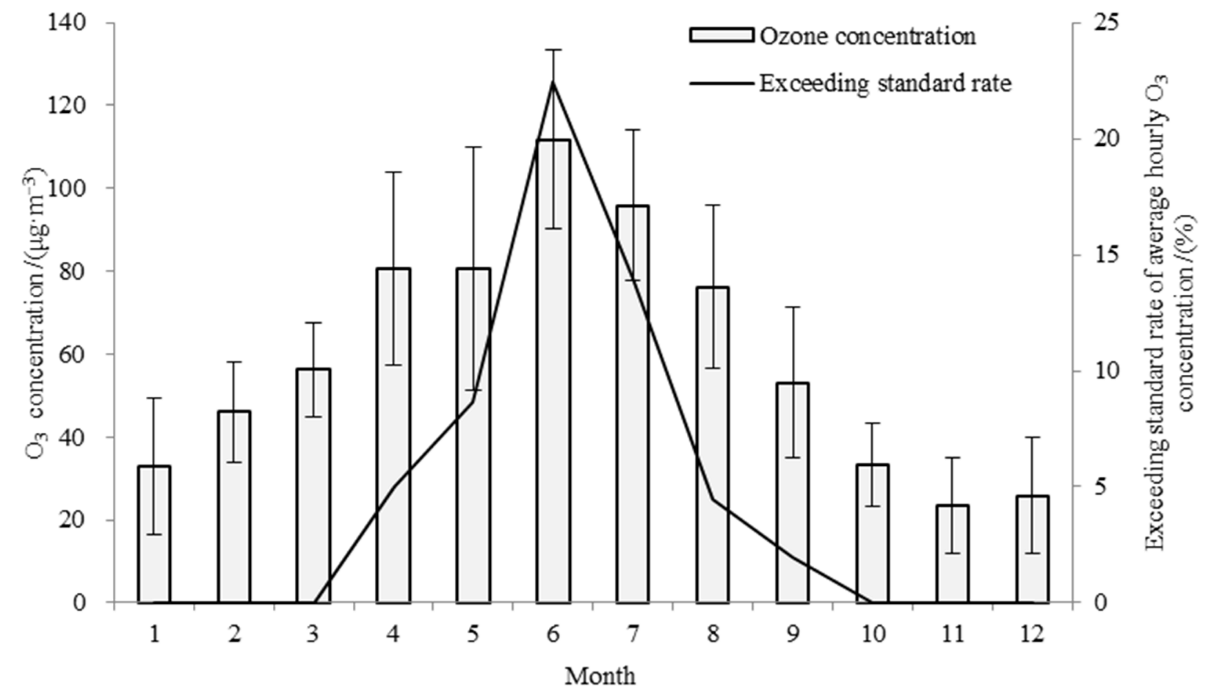
The monthly average O
3 concentration (
Figure 2) increased from January to June (cumulative increase of 238.6%), reached a peak value in June (111.73 μg·m
−3) and then declined to the end of the year. The rate of increase from March to April (+43.2%) was larger than the rate of increase from May to June (+38.7%). The lowest concentrations in January and December were 23.45 and 25.79 μg·m
−3, respectively.
In terms of the daily maximum 8 h average O
3 concentration, the highest values occurred in May to October (
Figure 3). The seasonal order of the average O
3 concentration in Beijing in 2020 was as follows: summer (95.04 μg·m
−3) > spring (72.99 μg·m
−3) > autumn (36.94 μg·m
−3) > winter (35.10 μg·m
−3). Hence the general pattern of daily maximum 8 h average O
3 concentration was high in spring and summer and low in autumn and winter.
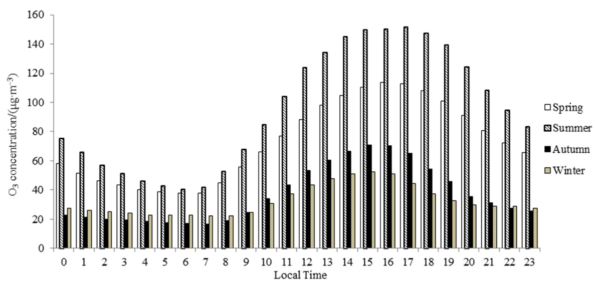
There was a significant diurnal variation of O
3 concentration (
Figure 4), with a similar diurnal pattern of O
3 concentration in all four seasons, i.e., low in the early morning, high in the afternoon. The average across all monitoring stations in the city exhibited a peak value of O
3 concentration between 13:00 and 18:00, and minimum values between 01:00 and 08:00 and 19:00 and 24:00.
The diurnal variation in each of the four annual seasons was slightly different. Compared with autumn and winter, the daily peaks in spring and summer were later in the day, i.e., 15:00 in autumn and winter and 17:00 in spring and summer. In addition, the fluctuation of O3 concentration was more significant in spring and summer and less in autumn and winter, especially at night. Hourly average O3 concentrations in summer were higher than those in other seasons, followed by those in spring. Average O3 concentrations in autumn were slightly lower than those in winter between 00:00 and 08:00, but higher in other time periods.
There was a clear weekly trend of daily mean O
3 concentrations (
Table 1). Daily average O
3 concentrations in Beijing were at high levels on Fridays (61.37 ± 26.89 μg·m
−3), Saturdays (61.46 ± 27.18 μg·m
−3) and Sundays (61.05 ± 23.83 μg·m
−3). In the spring, the concentrations of O
3 were highest on Thursdays and Fridays, and the lowest on Mondays, with the highest difference being 93.52%. The highest average values of daily mean O
3 concentration in summer appeared on weekends, although the higher values in autumn and winter appeared on Sundays and Mondays.
On the whole, average daily mean values on weekends were generally higher than those from working days. By selecting consecutive days (non-holidays) with similar weather conditions in representative months for analysis, it was found that the daily mean O3 concentration of weekends in Beijing was generally higher than those of working days, with the lowest daily average O3 concentrations on Wednesdays and Thursdays and highest on Saturdays and Sundays. Weekend restrictions in Beijing have led to the greater use of motor vehicles than during working days. This may increase the emission of O3 precursors and may also closely result in changes to the surrounding climate and environment. Within Beijing’s 5th Ring Road, motor vehicles are restricted according to the last number of their license plate. For example, vehicles with tail numbers 1 and 6, 2 and 7, 3 and 8, 4 and 9, 5 and 0 are banned on Monday, Tuesday, Wednesday, Thursday and Friday, respectively. However, there are no restrictions at weekends. Therefore, on working days, public transport is more heavily used than at weekends. This most likely reduces the emission of ozone precursors during the week to some extent.
3.2. Spatial Variation
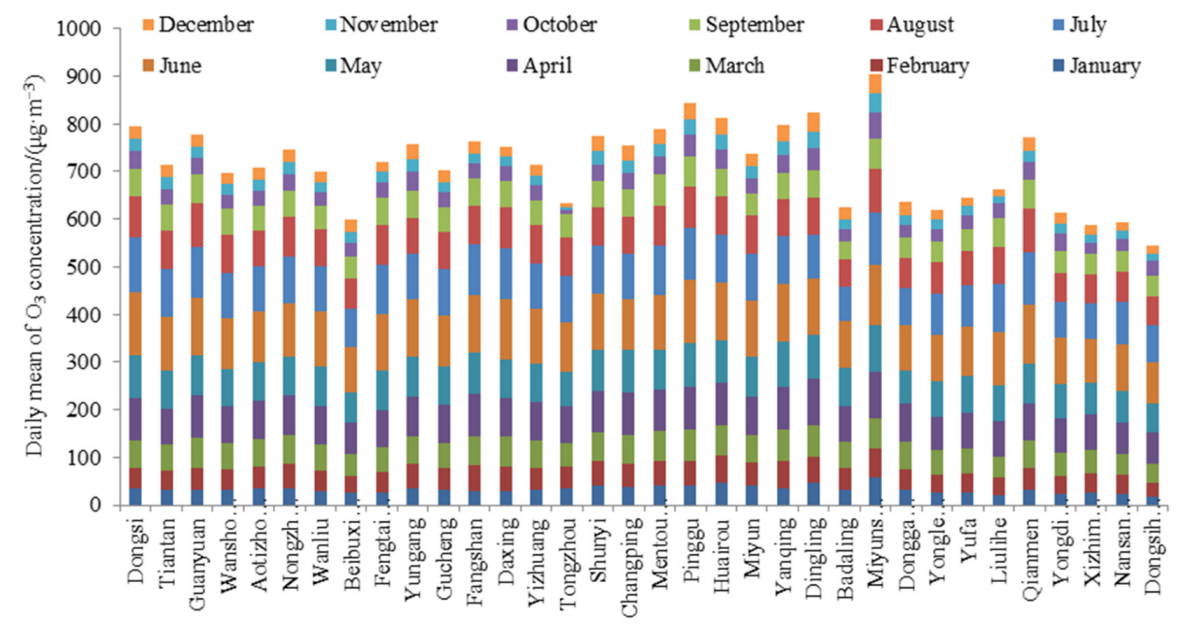
The highest annual average O
3 concentration at the 34 monitoring stations was at the Miyunshuiku Station (75.21 ± 44.36 μg·m
−3), followed by that at the Pinggu Station (70.04 ± 49.58 μg·m
−3) (
Figure 5). The lowest mean value was at the Dongsihuan Station (45.42 ± 45.45 μg·m
−3), followed by the Xizhimenbei Station (49.29 ± 41.65 μg·m
−3) and the Nansanhuan Station (49.47 ± 44.44 μg·m
−3).
Figure 6 shows the distribution of annual mean O
3 concentration at 35 stations fitted using Kriging interpolation. From the perspective of the whole city, the average annual O
3 concentration had slightly higher values in the northeast, southwest and northwest, and slightly lower values in the southeast. The 34 monitoring stations were grouped into six city regions according to their geographical location, i.e., six central districts (1–17); a northwest region (24, 29–31); a northeast region (23, 26–28, 32 and 33); a southwest region (19, 25 and 36); and a southeast region (20–22, 34 and 35). The values of the annual average O
3 concentrations in the six regions were ranked as follows: northeast region (65.37 ± 24.68 μg·m
−3) > northwest region (62.54 ± 23.21 μg·m
−3) > southwest region (61.53 ± 27.05 μg·m
−3) > central six districts (57.33 ± 25.06 μg·m
−3). By administrative area, the Miyun District had the highest annual average O
3 concentration, which was 29.52% higher than that of the Haidian District. On the whole, annual average O
3 concentrations in Beijing were higher in the suburbs than in central areas.
The spatial distribution of O
3 changes with different seasons. The highest seasonal average O
3 concentration in spring (
Table 2) was in the northwest region (79.62 ± 6.03 μg·m
−3). However, the highest seasonal average value in summer was in the southwest region (100.2 ± 6.24 μg·m
−3). The highest seasonal average O
3 concentrations in autumn and winter were in the northeast region (41.29 ± 7.75 and 42.45 ± 5.81 μg·m
−3, respectively). The seasonal average O
3 concentration in the southwest region showed the greatest difference between seasons.
3.3. Correlation between O3 Concentration and Meteorological Factors
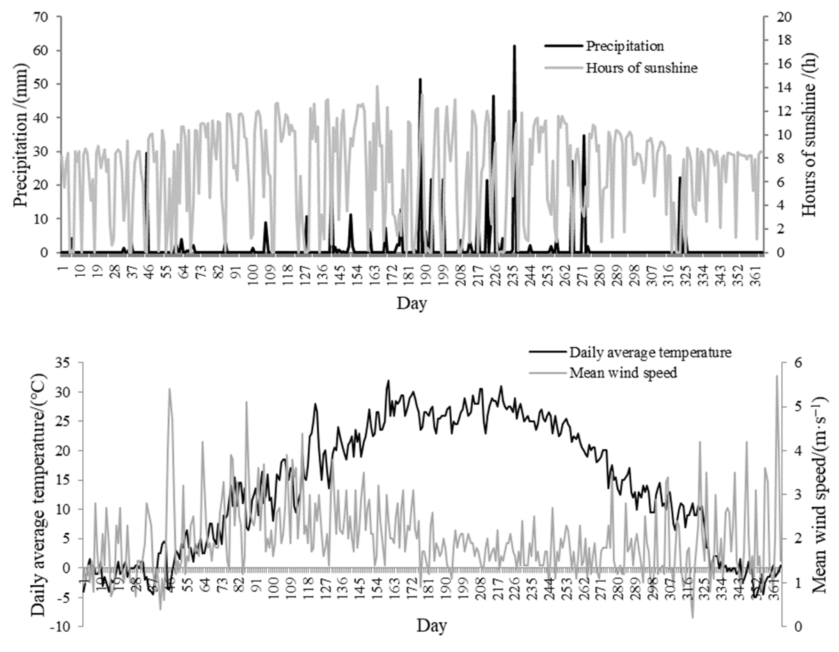
The daily meteorological data are summarized in
Figure 7. No significant correlation was found between O
3 concentration and precipitation (
p > 0.05.
Table 3), but there were significant correlations between O
3 concentration and average wind speed, sunshine hours and temperature (
p < 0.05). The correlation between O
3 concentration and average wind speed was relatively weak, while the highest correlation was between O
3 concentration and daily maximum temperature.
With increasing precipitation and sunshine hours (
Figure 8), the O
3 concentration decreased at first and then increased. When daily precipitation was in the range 50–60 mm, the daily average value of O
3 concentration was the highest (99.41 μg·m
−3). Contrarily, the daily average O
3 concentration was the lowest (37.17 μg·m
−3) when the daily precipitation was in the range 30–35 mm. When daily sunshine hours were more than 13 h, the daily average value O
3 concentration was highest (95.72 μg·m
−3). With increasing wind speed, the O
3 concentration first increased and then slowly decreased, with the rising rate being greater than the falling rate. When the wind speed was 2.5–3.0 m·s
−1, the daily average O
3 concentration reached the maximum value (75.32 μg·m
−3). With increasing temperature, the average O
3 concentration also increased. When the temperature was higher than 35 °C, the average value of O
3 concentration was the highest (119.12 μg·m
−3). When the highest temperature was between 0 and 5 °C and the lowest temperature was between 10 and 5 °C, the average value of O
3 concentration reached the lowest values (30.68 and 32.99 μg·m
−3, respectively). From the trend of temperature change throughout the year (
Figure 8), higher temperature values in Beijing appeared from May to October, which is consistent with the trend of O
3 concentration. From these results, it is clear that temperature is one of the more important factors affecting O
3 concentration in Beijing.
3.4. Correlation between O3 Concentration and Other Pollutants
As the product of the photochemical reaction, the concentration of O
3 is closely related to other polluting gases in the atmosphere. In 2020, there was a significant negative correlation between O
3 concentrations and NO
2 concentrations and CO concentrations in Beijing (
Table 4,
p < 0.001), with correlation coefficients of −0.553 and −0.159, respectively. There was a significant positive correlation with SO
2 concentration (0.001 <
p < 0.05).
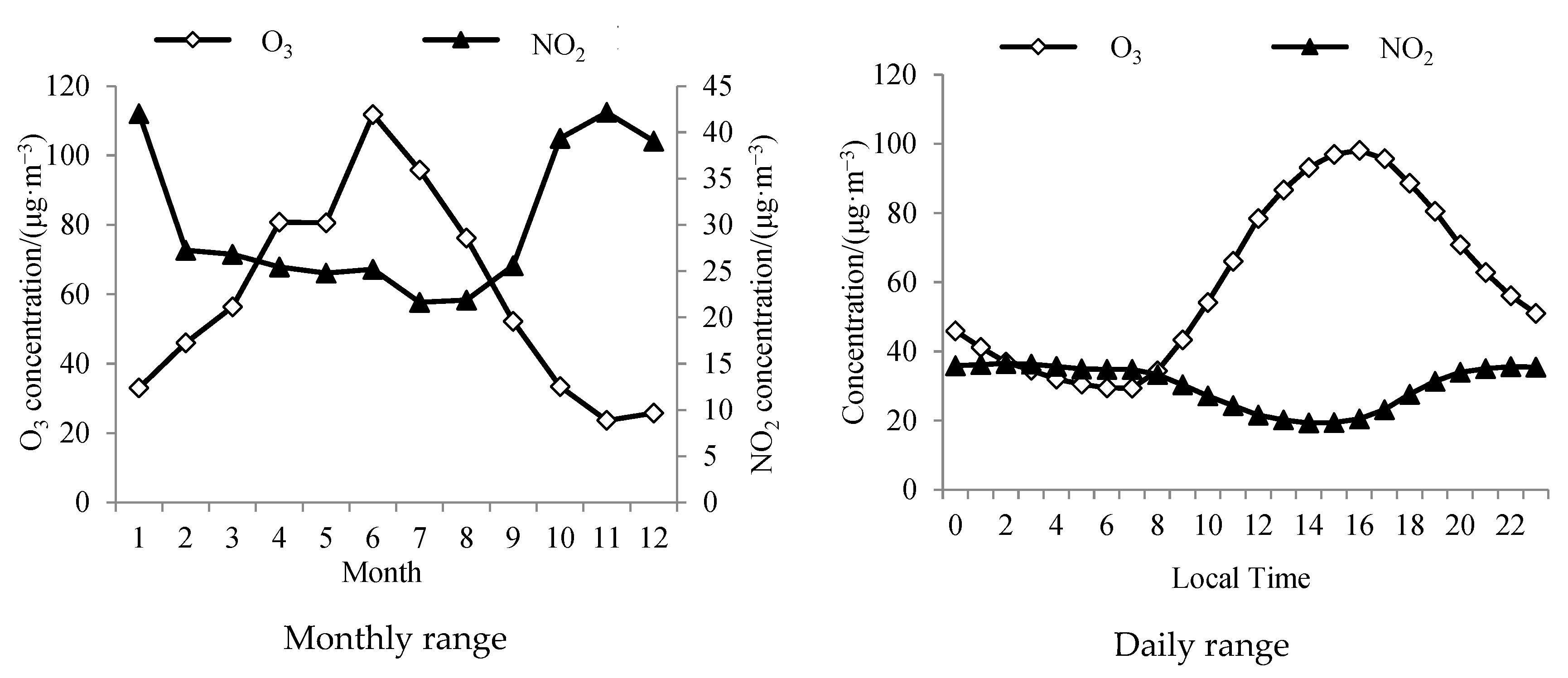
The correlation between O
3 and its precursor NO
2 is shown in
Figure 9. Monthly average values of O
3 concentration show a trend of first increasing and then decreasing through the year, reaching a maximum value in June, followed by July, and lowest value in November. However, the concentration of monthly average NO
2 concentration decreases first and then increases, reaching a minimum in July and a maximum in November. This appears to be related to the requirement for winter heating in Beijing.
In terms of diurnal variation, hourly O3 concentrations decreased through the night, gradually increased after sunrise, then reached a peak at 16:00 local time, falling back to a minimum at 06:00. However, the hourly NO2 concentration increased slowly at night and remained at a relatively stable high value until about 08:00, when it gradually decreased to the lowest value at 14:00. These trends are most likely due to the photochemical properties of the two gases. As the solar radiation disappears at night, the ground radiation is weak, and the temperature decreases. NO2 gradually accumulates until the solar radiation increases after sunrise, when NO2 gradually decomposes and is consumed, and the O3 content increases.
4. Discussion
4.1. Spatial-Temporal Dynamic Pattern of O3 Pollution
According to the statistics of the Bureau of Ecology and Environment, the average values of the maximum 8 h sliding average O3 concentration from 2016 to 2019 were 190, 193, 192 and 191 μg·m−3, respectively. Compared with the past 4 years, the O3 concentrations were lower in 2020, but the annual average was still high. On a seasonal scale, the seasonal variation of O3 concentration was remarkable, with the highest values in summer and the lowest in winter. On a daily time scale, the O3 concentration showed a single peak between 13:00 and 18:00.
The most important influencing factor of seasonal and daily variations was temperature. Previous research has shown that the higher the temperature, the higher the O
3 concentration generally [
31], which is most clear in the daily variation [
32]. The highest values of O
3 concentration observed in Beijing in this study in a day were in the afternoon, corresponding to the period of highest temperature, and gradually decreased with cooling nighttime temperatures.
In terms of annual variation, the highest values of O3 concentration appeared in June, followed by July. On the one hand, the average temperature in Beijing in June 2020 reached 27.12 °C, which was higher than that in July and August (26.56 and 26.51 °C, respectively), indicating that there was a certain correlation between temperature and O3 concentration. On the other hand, O3 concentrations were also related to the shortening of sunshine hours caused by rainy weather in July, August and September. With the shortening of sunshine hours and the decrease in solar radiation, the photochemical reactions of nitrogen oxides (NOx) and volatile organic compounds (VOCs) slow down. Southeast winds prevail in summer, compared to the clean air mass from Mongolia in winter, and these winds are more likely to be polluted by the production in eastern cities with high population density.
In terms of weekly variation, Cleveland first put forward the concept of a “weekend effect” in the variation of daily O
3 concentrations, suggesting that the concentration level of some O
3 precursors (such as VOC
s, CO and NO
x) decreased at the weekend but the concentration of O
3 increased significantly [
33]. On a weekly time scale, the daily O
3 average concentrations in Beijing showed a certain weekend effect, with slightly higher values than during weekdays. This is consistent with many existing research results on the weekly variation of O
3 [
34,
35]. Shi Yuzhen suggested that the reason for the O
3 “weekend effect” in Beijing is that the concentration of NO
x in weekend mornings is lower than that during working days [
36].
In terms of spatial distribution, O
3 in Beijing showed different characteristics from other pollutants, such as NO
2, PM
2.5 and PM
10. Geographically, O
3 concentrations were higher in the north and southwest and lowest in the southeast. From the perspective of urban development, concentration values were characterized by being lower in urban areas and higher in the suburbs. This dual pattern distribution was mainly due to the fact that volatile organic compounds can be roughly divided into natural sources and human-made sources, and more than 65% of non-methane volatile organic compounds in the world come from plant-based emissions every year [
37]. Some studies have pointed out that the quantities of plant-derived volatile organic compounds (BVOCs) emitted from the Miyun, Yanqing and Changping districts are the highest, together accounting for 35.23% of the city’s emissions [
38]. BVOCs are one of the important precursors of O
3, and so the O
3 concentration remained high in the former region, while the concentration in the southeast region was low.
The emission of volatile organic compounds from human-made sources is higher in urban areas, but the O
3 concentration is lower than that in suburban areas, which may be related to the consumption of O
3 by NO
2 emissions [
39]. In addition, the spatial pattern of O
3 distribution may also be related to the topography and prevailing wind direction of Beijing. Based on the analysis of the topographic elevation data of Beijing and the spatial location of monitoring points, it is found that the O
3 concentration is low in the flat and open areas in the southeast, while the northern areas, especially the Miyun and Huairou areas, are in relatively closed terrain, which makes it difficult for O
3 to spread. According to the statistics of wind direction, the frequency of southwestern wind is very high in spring, summer and autumn. When Beijing is under the influence of southerly winds and westerly winds, the O
3 concentration is relatively high in the north and east of the city. This is because the precursors from the south of Beijing are transported to the northeast.
4.2. Relationship between O3 Concentration and Meteorological Factors and Other Pollutants
There was a significant positive correlation (
p < 0.001) between the O
3 concentration and temperature and wind speed. It is concluded that the annual average correlation coefficients of O
3, NO, NO
2 and CO volume fraction and wind speed in Beijing were 0.49, −0.41, −0.49 and −0.38, respectively, although only O
3 was significantly correlated with wind speed [
40]. The correlation with temperature was the highest. When temperature increases, the ultraviolet intensity increases, and so the temperature is an important condition for O
3 generation.
Wind speed affects the O
3 concentration in Beijing. Higher wind speeds imply greater air pressure differences between adjacent areas, and strong vertical turbulence often occurs. Higher wind speed changes the surface air pressure. Fast wind will raise the height of the atmospheric boundary layer, causing upper O
3 to flow to the ground. At the same time, higher wind speed also diffuses surface O
3. The turbulent exchange between upper and lower atmospheric layers results in the wind speed being positively correlated with near-surface O
3, while horizontal diffusion makes them negatively correlated [
41].
There was a significant correlation between O3 concentration and sunshine hours in Beijing (p < 0.05), but no significant correlation between O3 concentration and precipitation (p > 0.05). The long sunshine hours give sufficient radiation for chemical reactions involving NOx and VOCs. Seasonal variation in O3 concentration is closely related to that of temperature, sunshine hours and wind speed, while daily temperature variation and human production activities affect the O3 concentration during a day, and the influence of human activities is the most prominent in the weekly variation.
Wind direction and human activities have a great influence on the spatial variation. When the southeast, south and west wind prevails in Beijing, it is easy to cause high O
3 pollution [
40,
42]. North airflow comes from Inner Mongolia and generally represents clean air. Southeast airflow comes from Bohai Bay, it originally belonged to a relatively clean ocean air mass, but before reaching Beijing, it was affected by severe air pollution in Tangshan and other cities.
In 2020, there was a significant correlation between O
3 concentration, NO
2 concentration and CO concentration in Beijing (
p < 0.001) and SO
2 concentration (0.001 <
p > 0.05). The correlation between O
3 concentration and NO
2 was the highest (−0.553), and there was a significant negative correlation between daily variation and monthly variation. This is consistent with previous analyses of long-term monitoring [
43,
44], which suggests that O
3 is closely related to NO
2, and the accumulation and decomposition of NO
2 has a very important influence on the formation of O
3 [
15].
4.3. Source and Prevention of O3 Pollution
O
3 pollution is a kind of secondary pollution, and its precursors are mainly NO
x and VOC
s. NO
x is mainly a human-made emission, mostly from automobile exhaust and the combustion of coal and oil, as well as a little from natural lightning. VOC
s have two sources, natural and human-made. Natural sources include volatile organic compounds released by plants, which sometimes leads to high O
3 concentrations in places with lush forest vegetation. Human-made sources include VOCs emitted from various human production activities, such as the coal-based chemical industry, the petrochemical industry, fuel coating manufacturing and solvent manufacturing. Volatile organic compounds emitted from human-made sources are the main causes of urban photochemical pollution [
45].
O
3 pollution, although closely related to temperature, sunshine hours and wind speed under specific conditions, is also affected by human activities, which can influence the daily and weekly variations of O
3. In addition to local photochemical smog, pollutants in the surrounding areas also affect the O
3 concentration in Beijing along with the long-distance input of air flow. Under the influence of air flow from the southeast, south and west, polluted air flow from Tianjin, Hebei and other places will also gather here. A simulation study of O
3 pollution in Beijing by Streets [
46] found that the contribution of pollution sources from surrounding areas to O
3 concentrations in Beijing is between 35% and 60%.
At present, the prevention and control of O3 pollution in Beijing mainly focuses on monitoring, early warning and controlling the emission of precursors. As O3 is an imperceptible pollution, monitoring and early warning of ozone play a very important societal role. It is also necessary to effectively control the emission of volatile organic compounds and nitrogen oxides, such as using clean energy, controlling the number of motor vehicles, improving industrial processes and promoting clean production. As the relationship between O3 and NOx and VOCs is further demonstrated, the emission reduction of NOx and VOCs should be verified through studies and more efficient prevention and control measures implemented. As O3 is transported between regions, the prevention and control of O3 pollution need to develop from local control to regional joint prevention and control.


