
Generating Fine-Scale Aerosol Data through Downscaling with an Artificial Neural Network Enhanced with Transfer Learning


Abstract
:1. Introduction
2. Materials and Methods
2.1. Data
2.1.1. MERRA-2
2.1.2. G5NR
2.1.3. GMTED2010 Elevation
2.2. Downscaling Model
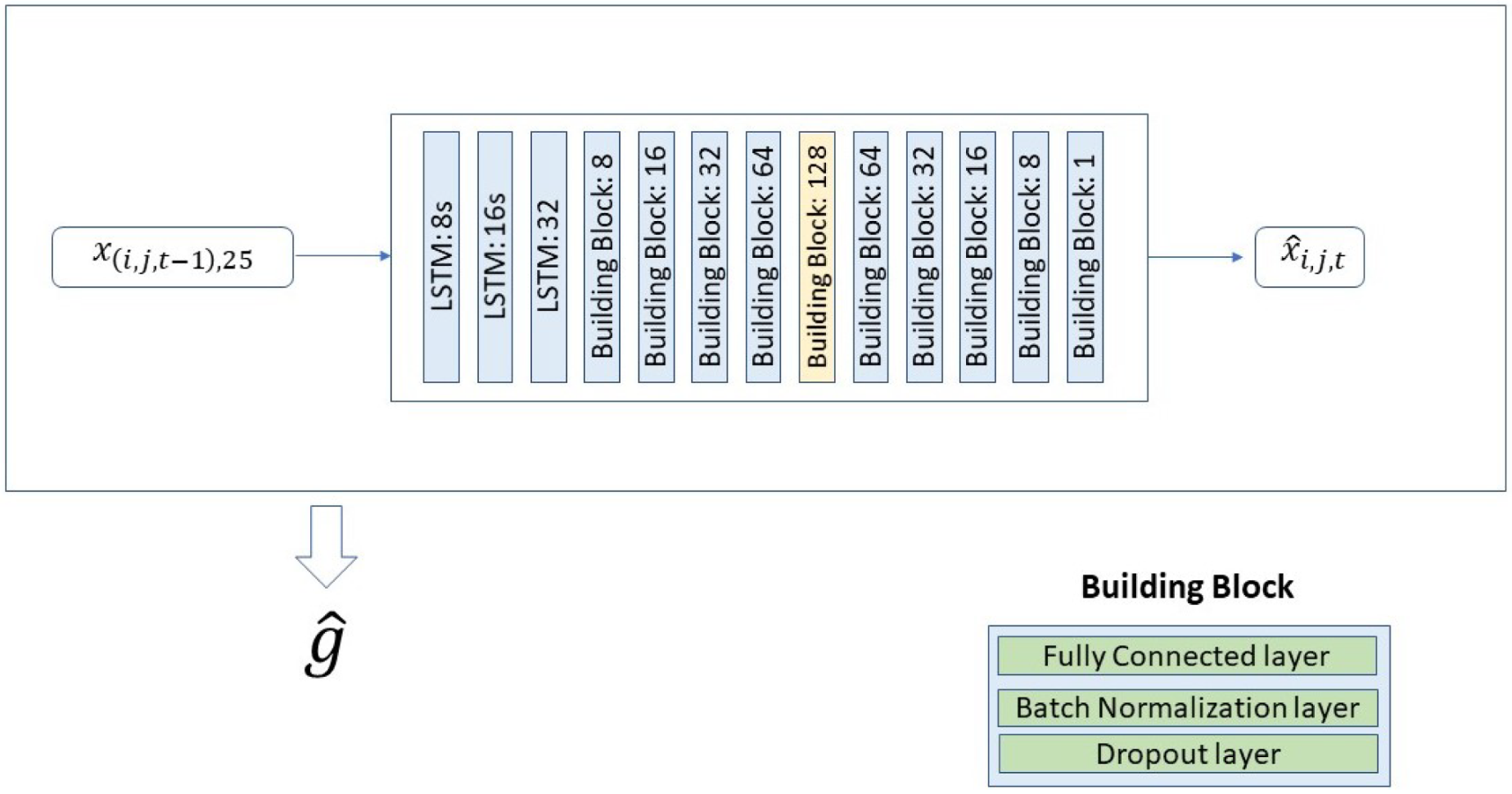
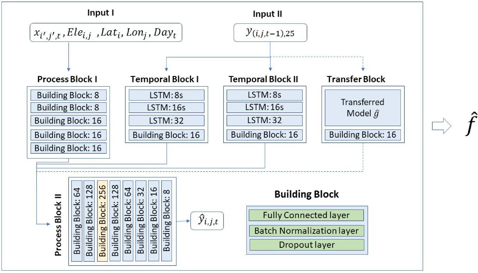
2.2.1. ASDM/ASDMTE Network Structure
2.2.2. Transferred Model
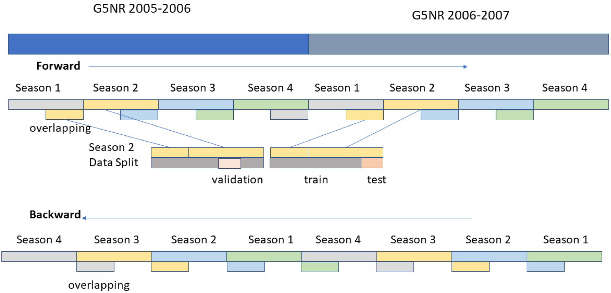
2.2.3. Training Strategy
2.2.4. Evaluation
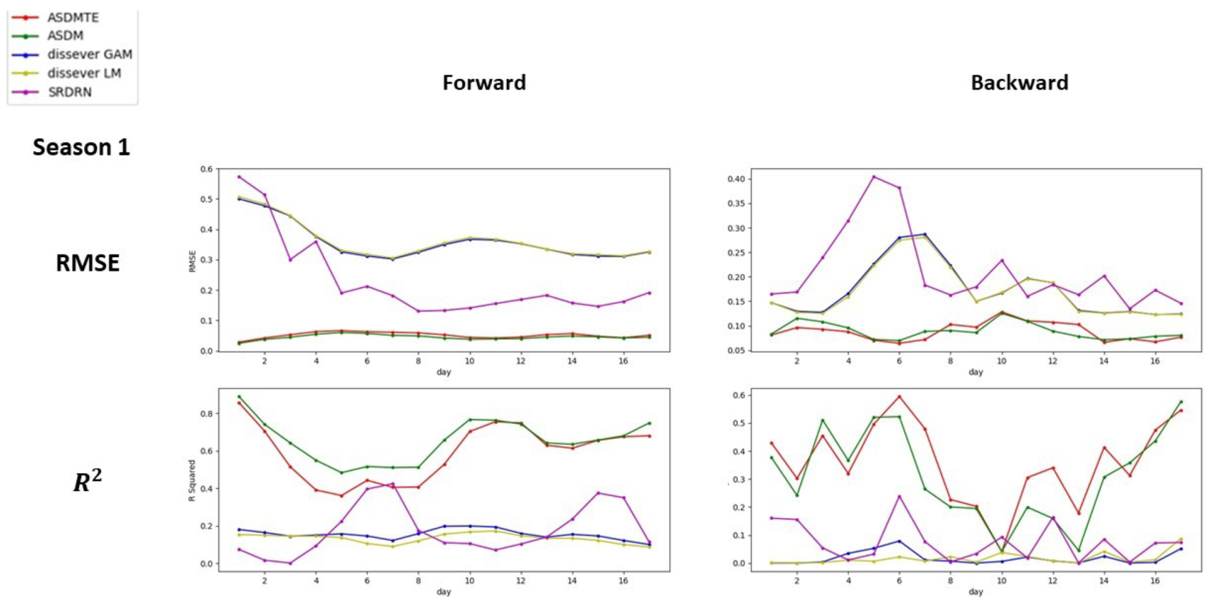
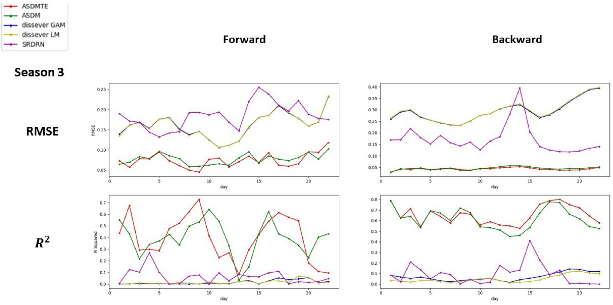
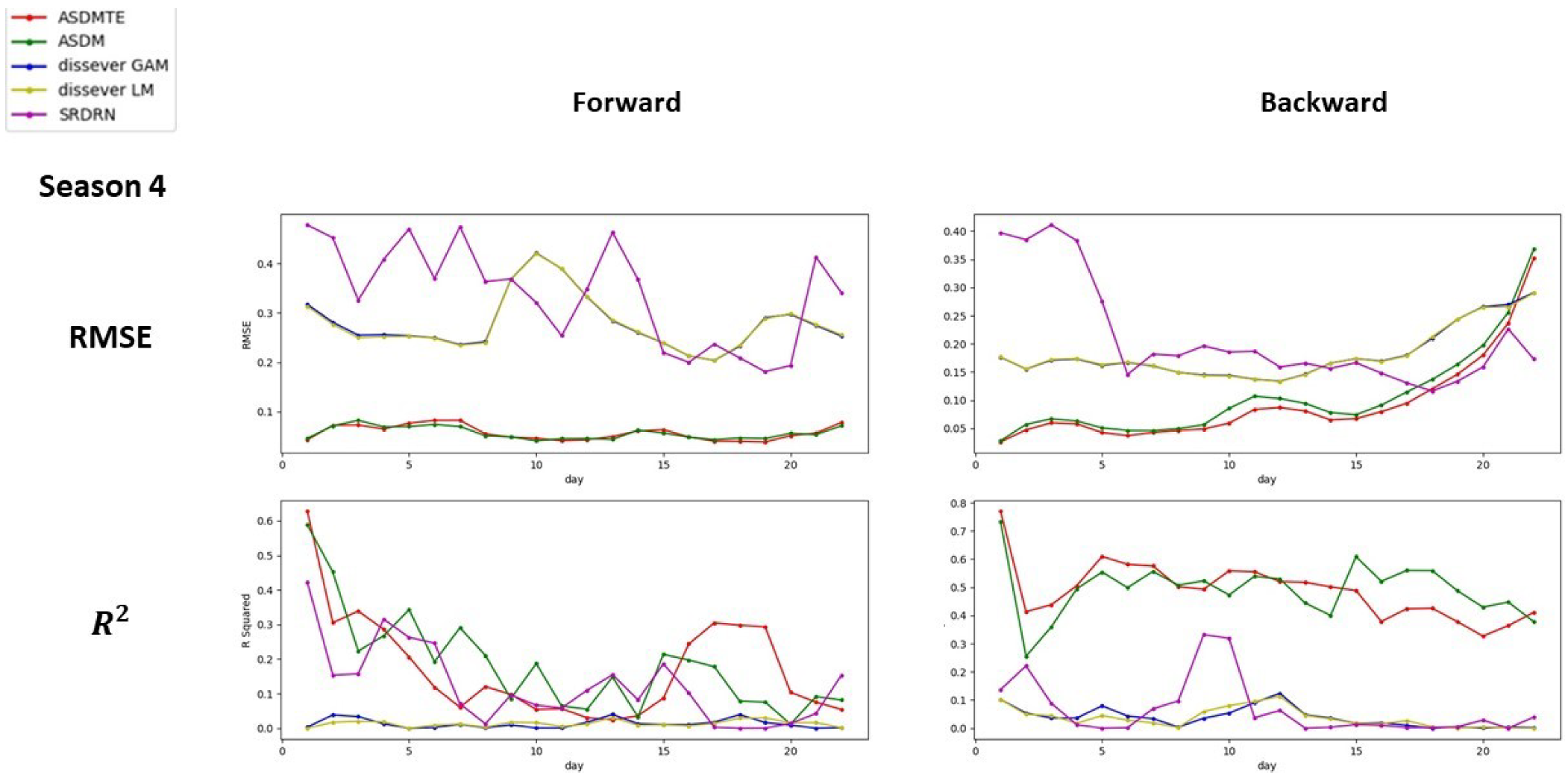
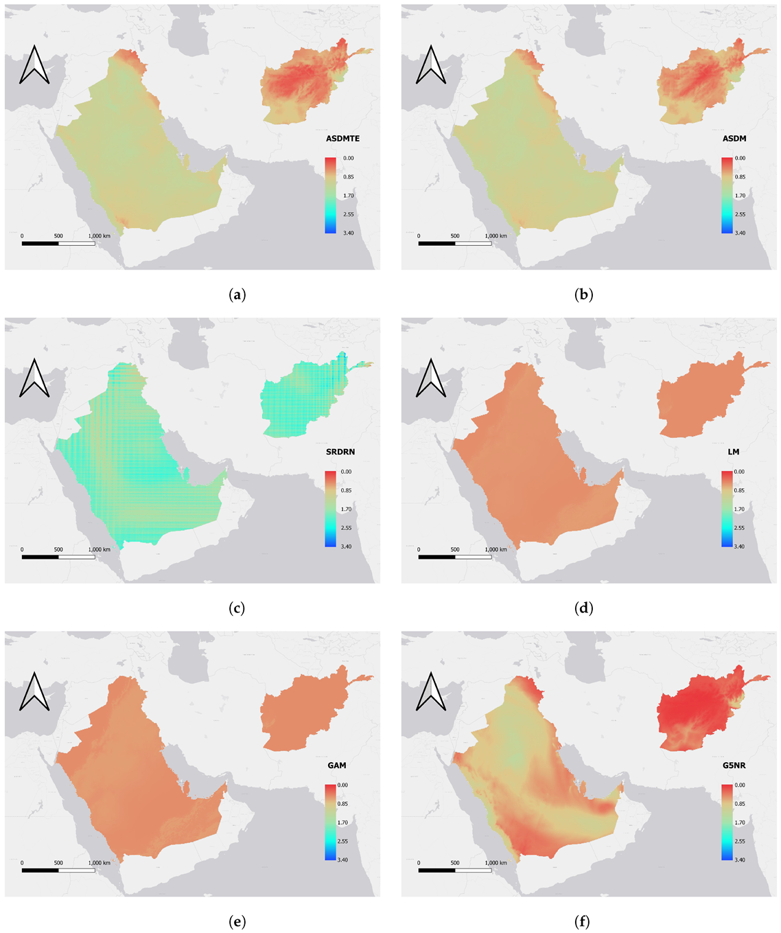
3. Results
4. Discussion
Author Contributions
Funding
Institutional Review Board Statement
Informed Consent Statement
Data Availability Statement
Conflicts of Interest
Abbreviations
| ANN | Artificial Neural Network |
| AOD | Aerosol Optical Depth |
| ASDM | Artificial Neural Network Sequentially Downscaling Method |
| ASDMTE | ASDM with Transfer Learning Enhancement |
| CNN | Convolutional Neural Netwrok |
| CS | Coarse-Scale |
| ECMWF | European Centre for Medium-Range Weather Forecasts |
| FC | Fully Connected |
| FS | Fine-Scale |
| G5NR | GEOS-5 Nature Run |
| GAM | Generalized Additive Model |
| GCM | General Circulation Model |
| GEOS-5 | Goddard Earth Observing System Model, Version 5 |
| GEOS-5 AGCM | GEOS-5 Atmospheric General Circulation Model |
| GMAO | Global Modeling and Assimilation Of-44fice |
| GMTED2010 | The Global Multi-resolution Terrain Elevation Data 2010 |
| LM | Linear Regression Model |
| MERRA-2 | Modern-Era Retrospective analysis for8Research and Applications, Version 2 |
| MSE | Mean Square Error |
| NGA | Geospatial-Intelligence Agency |
| OSSEs | Observing System Simulation Experiments |
| ReLU | Rectified Linear Unit |
| RMSE | Root Mean Square Error |
| SD | Standard Deviation |
| SRDRN | Super Resolution Deep Residual Network |
| USGS | U.S. Geological Survey |
| UAE | United Arab Emirates |
Appendix A. Supplemental Results: Downscaling Performance

References
- Chudnovsky, A.; Lyapustin, A.; Wang, Y.; Tang, C.; Schwartz, J.; Koutrakis, P. High resolution aerosol data from MODIS satellite for urban air quality studies. Open Geosci. 2014, 6, 17–26. [Google Scholar] [CrossRef] [Green Version]
- Kloog, I.; Chudnovsky, A.A.; Just, A.C.; Nordio, F.; Koutrakis, P.; Coull, B.A.; Lyapustin, A.; Wang, Y.; Schwartz, J. A new hybrid spatio-temporal model for estimating daily multi-year PM2. 5 concentrations across northeastern USA using high resolution aerosol optical depth data. Atmos. Environ. 2014, 95, 581–590. [Google Scholar] [CrossRef] [PubMed] [Green Version]
- Li, L.; Girguis, M.; Lurmann, F.; Pavlovic, N.; McClure, C.; Franklin, M.; Wu, J.; Oman, L.D.; Breton, C.; Gilliland, F.; et al. Ensemble-based deep learning for estimating PM2.5 over California with multisource big data including wildfire smoke. Environ. Int. 2020, 145, 106143. [Google Scholar] [CrossRef]
- Zheng, C.; Zhao, C.; Zhu, Y.; Wang, Y.; Shi, X.; Wu, X.; Chen, T.; Wu, F.; Qiu, Y. Analysis of influential factors for the relationship between PM2.5 and AOD in Beijing. Atmos. Chem. Phys. 2017, 17, 13473–13489. [Google Scholar] [CrossRef] [Green Version]
- Xing, Y.F.; Xu, Y.H.; Shi, M.H.; Lian, Y.X. The impact of PM2.5 on the human respiratory system. J. Thorac. Dis. 2016, 8, E69. [Google Scholar] [PubMed]
- Choi, J.; Oh, J.Y.; Lee, Y.S.; Min, K.H.; Hur, G.Y.; Lee, S.Y.; Kang, K.H.; Shim, J.J. Harmful impact of air pollution on severe acute exacerbation of chronic obstructive pulmonary disease: Particulate matter is hazardous. Int. J. Chronic Obstr. Pulm. Dis. 2018, 13, 1053. [Google Scholar] [CrossRef] [PubMed] [Green Version]
- Chau, K.; Franklin, M.; Gauderman, W.J. Satellite-Derived PM2.5 Composition and Its Differential Effect on Children’s Lung Function. Remote Sens. 2020, 12, 1028. [Google Scholar] [CrossRef] [Green Version]
- Maji, S.; Ghosh, S.; Ahmed, S. Association of air quality with respiratory and cardiovascular morbidity rate in Delhi, India. Int. J. Environ. Health Res. 2018, 28, 471–490. [Google Scholar] [CrossRef]
- Franklin, M.; Chau, K.; Kalashnikova, O.V.; Garay, M.J.; Enebish, T.; Sorek-Hamer, M. Using multi-angle imaging spectroradiometer aerosol mixture properties for air quality assessment in Mongolia. Remote Sens. 2018, 10, 1317. [Google Scholar] [CrossRef] [Green Version]
- Franklin, M.; Kalashnikova, O.V.; Garay, M.J. Size-resolved particulate matter concentrations derived from 4.4km-resolution size-fractionated Multi-angle Imaging SpectroRadiometer (MISR) aerosol optical depth over Southern California. Remote Sens. Environ. 2017, 196, 312–323. [Google Scholar] [CrossRef]
- Farzanegan, M.R.; Markwardt, G. Development and pollution in the Middle East and North Africa: Democracy matters. J. Policy Model. 2018, 40, 350–374. [Google Scholar] [CrossRef]
- Chau, K.; Franklin, M.; Lee, H.; Garay, M. Temporal and Spatial Autocorrelation as Determinants of Regional AOD-PM 2 . 5 Model Performance in the Middle East. Remote Sens. 2021, 13, 3790. [Google Scholar] [CrossRef]
- Li, J.; Garshick, E.; Hart, J.E.; Li, L.; Shi, L.; Al-Hemoud, A.; Huang, S.; Koutrakis, P. Estimation of ambient PM2.5 in Iraq and Kuwait from 2001 to 2018 using machine learning and remote sensing. Environ. Int. 2021, 151, 106445. [Google Scholar] [CrossRef] [PubMed]
- Sun, E.; Xu, X.; Che, H.; Tang, Z.; Gui, K.; An, L.; Lu, C.; Shi, G. Variation in MERRA-2 aerosol optical depth and absorption aerosol optical depth over China from 1980 to 2017. J. Atmos. Sol.-Terr. Phys. 2019, 186, 8–19. [Google Scholar] [CrossRef]
- Ukhov, A.; Mostamandi, S.; da Silva, A.; Flemming, J.; Alshehri, Y.; Shevchenko, I.; Stenchikov, G. Assessment of natural and anthropogenic aerosol air pollution in the Middle East using MERRA-2, CAMS data assimilation products, and high-resolution WRF-Chem model simulations. Atmos. Chem. Phys. 2020, 20, 9281–9310. [Google Scholar] [CrossRef]
- da Silva, A.M.; Putman, W.; Nattala, J. File Specification for the 7-km GEOS-5 Nature Run, Ganymed Release Non-Hydrostatic 7-km Global Mesoscale Simulation; Technical Report number GSFC-E-DAA-TN19; Global Modeling and Assimilation Office, Earth Sciences Division, NASA Goddard Space Flight Center: Greenbelt, MD, USA, 2014. Available online: https://ntrs.nasa.gov/api/citations/20150001439/downloads/20150001439.pdf (accessed on 29 December 2021).
- Wilby, R.L.; Wigley, T.; Conway, D.; Jones, P.; Hewitson, B.; Main, J.; Wilks, D. Statistical downscaling of general circulation model output: A comparison of methods. Water Resour. Res. 1998, 34, 2995–3008. [Google Scholar] [CrossRef]
- Malone, B.P.; McBratney, A.B.; Minasny, B.; Wheeler, I. A general method for downscaling earth resource information. Comput. Geosci. 2012, 41, 119–125. [Google Scholar] [CrossRef]
- Xu, Y.; Wang, L.; Ma, Z.; Li, B.; Bartels, R.; Liu, C.; Zhang, X.; Dong, J. Spatially explicit model for statistical downscaling of satellite passive microwave soil moisture. IEEE Trans. Geosci. Remote Sens. 2019, 58, 1182–1191. [Google Scholar] [CrossRef]
- Chang, H.H.; Hu, X.; Liu, Y. Calibrating MODIS aerosol optical depth for predicting daily PM 2.5 concentrations via statistical downscaling. J. Expo. Sci. Environ. Epidemiol. 2014, 24, 398–404. [Google Scholar] [CrossRef] [Green Version]
- Atkinson, P.M. Downscaling in remote sensing. Int. J. Appl. Earth Obs. Geoinf. 2013, 22, 106–114. [Google Scholar] [CrossRef]
- Wilby, R.L.; Charles, S.P.; Zorita, E.; Timbal, B.; Whetton, P.; Mearns, L.O. Guidelines for use of climate scenarios developed from statistical downscaling methods. Support. Mater. Intergov. Panel Clim. Chang. Available DDC IPCC TGCIA 2004, 27, 1–27. [Google Scholar]
- Goodfellow, I.; Bengio, Y.; Courville, A. Deep Learning; MIT Press: Cambridge, MA, USA, 2016. [Google Scholar]
- Yuan, Q.; Shen, H.; Li, T.; Li, Z.; Li, S.; Jiang, Y.; Xu, H.; Tan, W.; Yang, Q.; Wang, J.; et al. Deep learning in environmental remote sensing: Achievements and challenges. Remote Sens. Environ. 2020, 241, 111716. [Google Scholar] [CrossRef]
- Baño-Medina, J.; Manzanas, R.; Gutiérrez, J.M. Configuration and intercomparison of deep learning neural models for statistical downscaling. Geosci. Model Dev. 2020, 13, 2109–2124. [Google Scholar] [CrossRef]
- Wang, F.; Tian, D.; Lowe, L.; Kalin, L.; Lehrter, J. Deep Learning for Daily Precipitation and Temperature Downscaling. Water Resour. Res. 2021, 57, e2020WR029308. [Google Scholar] [CrossRef]
- Li, L.; Franklin, M.; Girguis, M.; Lurmann, F.; Wu, J.; Pavlovic, N.; Breton, C.; Gilliland, F.; Habre, R. Spatiotemporal imputation of MAIAC AOD using deep learning with downscaling. Remote Sens. Environ. 2020, 237, 111584. [Google Scholar] [CrossRef] [PubMed]
- Hidalgo, H.G.; Dettinger, M.D.; Cayan, D.R. Downscaling with Constructed Analogues: Daily Precipitation and Temperature Fields over the United States; California Energy Commission PIER Final Project Report CEC-500-2007-123; 2008. [Google Scholar]
- Agatonovic-Kustrin, S.; Beresford, R. Basic concepts of artificial neural network (ANN) modeling and its application in pharmaceutical research. J. Pharm. Biomed. Anal. 2000, 22, 717–727. [Google Scholar] [CrossRef]
- Gelaro, R.; McCarty, W.; Suárez, M.J.; Todling, R.; Molod, A.; Takacs, L.; Randles, C.A.; Darmenov, A.; Bosilovich, M.G.; Reichle, R.; et al. The modern-era retrospective analysis for research and applications, version 2 (MERRA-2). J. Clim. 2017, 30, 5419–5454. [Google Scholar] [CrossRef]
- Rienecker, M.M.; Suarez, M.; Todling, R.; Bacmeister, J.; Takacs, L.; Liu, H.; Gu, W.; Sienkiewicz, M.; Koster, R.; Gelaro, R.; et al. The GEOS-5 Data Assimilation System: Documentation of Versions 5.0. 1, 5.1. 0, and 5.2. 0. 2008. Available online: https://gmao.gsfc.nasa.gov/pubs/docs/Rienecker369.pdf (accessed on 29 December 2021).
- Molod, A.; Takacs, L.; Suarez, M.; Bacmeister, J. Development of the GEOS-5 atmospheric general circulation model: Evolution from MERRA to MERRA2. Geosci. Model Dev. 2015, 8, 1339–1356. [Google Scholar] [CrossRef] [Green Version]
- Wu, W.S.; Purser, R.J.; Parrish, D.F. Three-dimensional variational analysis with spatially inhomogeneous covariances. Mon. Weather Rev. 2002, 130, 2905–2916. [Google Scholar] [CrossRef] [Green Version]
- Kleist, D.T.; Parrish, D.F.; Derber, J.C.; Treadon, R.; Wu, W.S.; Lord, S. Introduction of the GSI into the NCEP global data assimilation system. Weather Forecast. 2009, 24, 1691–1705. [Google Scholar] [CrossRef] [Green Version]
- Koster, R.D.; McCarty, W.; Coy, L.; Gelaro, R.; Huang, A.; Merkova, D.; Smith, E.B.; Sienkiewicz, M.; Wargan, K. MERRA-2 Input Observations: Summary and Assessment. 2016. Available online: https://gmao.gsfc.nasa.gov/pubs/docs/McCarty885.pdf (accessed on 29 December 2021).
- Randles, C.A.; da Silva, A.M.; Buchard, V.; Colarco, P.R.; Darmenov, A.; Govindaraju, R.; Smirnov, A.; Holben, B.; Ferrare, R.; Hair, J.; et al. The MERRA-2 aerosol reanalysis, 1980 onward. Part I: System description and data assimilation evaluation. J. Clim. 2017, 30, 6823–6850. [Google Scholar] [CrossRef] [PubMed]
- Bosilovich, M.; Lucchesi, R.; Suarez, M. MERRA-2: File Specification. 2015. Available online: https://gmao.gsfc.nasa.gov/pubs/docs/Bosilovich785.pdf (accessed on 29 December 2021).
- Gelaro, R.; Putman, W.M.; Pawson, S.; Draper, C.; Molod, A.; Norris, P.M.; Ott, L.; Prive, N.; Reale, O.; Achuthavarier, D.; et al. Evaluation of the 7-km GEOS-5 Nature Run. 2015. Available online: https://ntrs.nasa.gov/api/citations/20150011486/downloads/20150011486.pdf (accessed on 29 December 2021).
- Danielson, J.J.; Gesch, D.B. Global Multi-Resolution Terrain Elevation Data 2010 (GMTED2010). 2011. Available online: https://pubs.usgs.gov/of/2011/1073/pdf/of2011-1073.pdf (accessed on 29 December 2021).
- Carabajal, C.C.; Harding, D.J.; Boy, J.P.; Danielson, J.J.; Gesch, D.B.; Suchdeo, V.P. Evaluation of the global multi-resolution terrain elevation data 2010 (GMTED2010) using ICESat geodetic control. In International Symposium on Lidar and Radar Mapping 2011: Technologies and Applications; International Society for Optics and Photonics: Bellingham, WA, USA, 2011; Volume 8286, p. 82861Y. [Google Scholar]
- Pan, S.J.; Yang, Q. A survey on transfer learning. IEEE Trans. Knowl. Data Eng. 2009, 22, 1345–1359. [Google Scholar] [CrossRef]
- Torrey, L.; Shavlik, J. Transfer learning. In Handbook of Research on Machine Learning Applications and Trends: Algorithms, Methods, and Techniques; IGI Publishing: 701 E. Chocolate Avenue, Suite 200, Hershey, PA, USA, 2010; pp. 242–264. [Google Scholar]
- Hochreiter, S.; Schmidhuber, J. Long short-term memory. Neural Comput. 1997, 9, 1735–1780. [Google Scholar] [CrossRef] [PubMed]
- Maas, A.L.; Hannun, A.Y.; Ng, A.Y. Rectifier nonlinearities improve neural network acoustic models. In Proceedings of the 30th International Conference on Machine Learning, Atlanta, GA, USA, 16–21 June 2013; Volume 28, pp. 1–6. [Google Scholar]
- Santurkar, S.; Tsipras, D.; Ilyas, A.; Mądry, A. How does batch normalization help optimization? In Proceedings of the 32nd International Conference on Neural Information Processing Systems (NeurIPS 2018), Montréal, QC, Canada, 3–8 December 2018; pp. 2488–2498. [Google Scholar]
- Ioffe, S.; Szegedy, C. Batch normalization: Accelerating deep network training by reducing internal covariate shift. In Proceedings of the International Conference on Machine Learning, PMLR, Lille France, 6–11 July 2015; pp. 448–456. [Google Scholar]
- Wager, S.; Wang, S.; Liang, P.S. Dropout training as adaptive regularization. Adv. Neural Inf. Process. Syst. 2013, 26, 351–359. [Google Scholar]
- Srivastava, N.; Hinton, G.; Krizhevsky, A.; Sutskever, I.; Salakhutdinov, R. Dropout: A simple way to prevent neural networks from overfitting. J. Mach. Learn. Res. 2014, 15, 1929–1958. [Google Scholar]
- Benestad, R.E.; Chen, D.; Hanssen-Bauer, I. Empirical-Statistical Downscaling; World Scientific Publishing Company: Singapore, 2008. [Google Scholar]
- Loew, A.; Mauser, W. On the disaggregation of passive microwave soil moisture data using a priori knowledge of temporally persistent soil moisture fields. IEEE Trans. Geosci. Remote Sens. 2008, 46, 819–834. [Google Scholar] [CrossRef]
- Wang, Y.; Sivandran, G.; Bielicki, J.M. The stationarity of two statistical downscaling methods for precipitation under different choices of cross-validation periods. Int. J. Climatol. 2018, 38, e330–e348. [Google Scholar] [CrossRef]
- Lanzante, J.R.; Dixon, K.W.; Nath, M.J.; Whitlock, C.E.; Adams-Smith, D. Some pitfalls in statistical downscaling of future climate. Bull. Am. Meteorol. Soc. 2018, 99, 791–803. [Google Scholar] [CrossRef]


| Method | Mean | Forward | Backward | |||||||
|---|---|---|---|---|---|---|---|---|---|---|
| Season 1 | Season 2 | Season 3 | Season 4 | Season 1 | Season 2 | Season 3 | Season 4 | |||
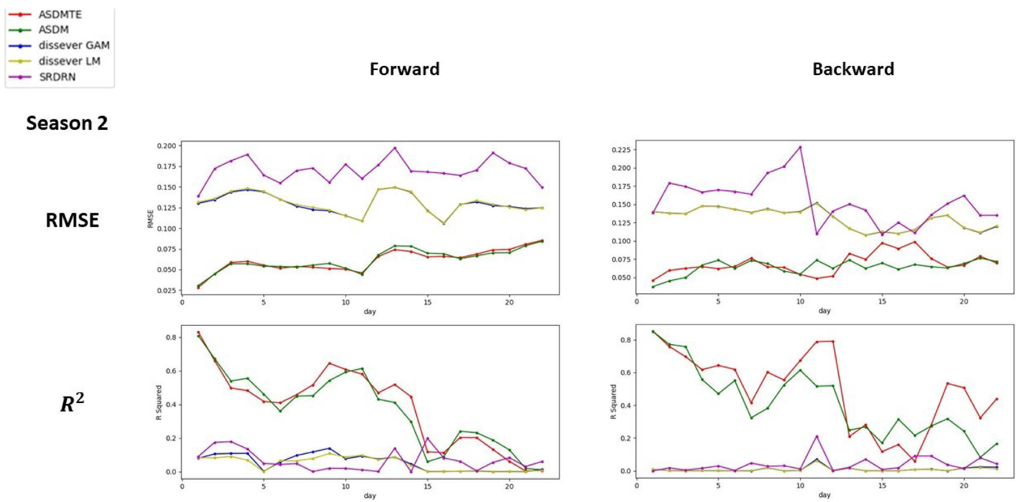
| ASDMTE | 0.758 (0.443) | 0.857 (0.593) | 0.831 (0.381) | 0.728 (0.396) | 0.628 (0.174) | 0.595 (0.360) | 0.851 (0.496) | 0.802 (0.653) | 0.770 (0.488) | |
| RMSE | 0.067 (0.021) | 0.051 (0.010) | 0.061 (0.013) | 0.074 (0.017) | 0.058 (0.014) | 0.088 (0.018) | 0.069 (0.014) | 0.043 (0.005) | 0.094 (0.075) | |
| ASDM | 0.735 (0.431) | 0.890 (0.656) | 0.810 (0.371) | 0.642 (0.394) | 0.588 (0.185) | 0.576 (0.313) | 0.851 (0.415) | 0.790 (0.616) | 0.732 (0.494) | |
| RMSE | 0.068 (0.020) | 0.045 (0.008) | 0.062 (0.013) | 0.077 (0.012) | 0.057 (0.012) | 0.089 (0.016) | 0.064 (0.010) | 0.045 (0.007) | 0.106 (0.078) | |
| SRDRN | 0.313 (0.088) | 0.425 (0.177) | 0.198 (0.067) | 0.268 (0.063) | 0.422 (0.123) | 0.239 (0.075) | 0.211 (0.040) | 0.412 (0.094) | 0.332 (0.067) | |
| RMSE | 0.088 (0.083) | 0.177 (0.131) | 0.067 (0.060) | 0.063 (0.060) | 0.123 (0.108) | 0.075 (0.067) | 0.040 (0.046) | 0.094 (0.098) | 0.067 (0.098) | |
| dissever GAM | 0.106 (0.046) | 0.199 (0.155) | 0.139 (0.055) | 0.056 (0.015) | 0.040 (0.013) | 0.079 (0.018) | 0.070 (0.009) | 0.143 (0.068) | 0.124 (0.038) | |
| RMSE | 0.213 (0.039) | 0.359 (0.058) | 0.130 (0.012) | 0.161 (0.030) | 0.280 (0.055) | 0.172 (0.052) | 0.131 (0.014) | 0.293 (0.045) | 0.181 (0.044) | |
| dissever LM | 0.095 (0.040) | 0.173 (0.133) | 0.108 (0.047) | 0.067 (0.015) | 0.031 (0.013) | 0.087 (0.017) | 0.062 (0.008) | 0.121 (0.048) | 0.113 (0.037) | |
| RMSE | 0.214 (0.039) | 0.362 (0.059) | 0.130 (0.012) | 0.161 (0.031) | 0.279 (0.055) | 0.170 (0.051) | 0.131 (0.013) | 0.295 (0.045) | 0.181 (0.044) | |
Publisher’s Note: MDPI stays neutral with regard to jurisdictional claims in published maps and institutional affiliations. |
© 2022 by the authors. Licensee MDPI, Basel, Switzerland. This article is an open access article distributed under the terms and conditions of the Creative Commons Attribution (CC BY) license (https://creativecommons.org/licenses/by/4.0/).
Share and Cite
Wang, M.; Franklin, M.; Li, L. Generating Fine-Scale Aerosol Data through Downscaling with an Artificial Neural Network Enhanced with Transfer Learning. Atmosphere 2022, 13, 255. https://doi.org/10.3390/atmos13020255
Wang M, Franklin M, Li L. Generating Fine-Scale Aerosol Data through Downscaling with an Artificial Neural Network Enhanced with Transfer Learning. Atmosphere. 2022; 13(2):255. https://doi.org/10.3390/atmos13020255
Chicago/Turabian StyleWang, Menglin, Meredith Franklin, and Lianfa Li. 2022. "Generating Fine-Scale Aerosol Data through Downscaling with an Artificial Neural Network Enhanced with Transfer Learning" Atmosphere 13, no. 2: 255. https://doi.org/10.3390/atmos13020255
APA StyleWang, M., Franklin, M., & Li, L. (2022). Generating Fine-Scale Aerosol Data through Downscaling with an Artificial Neural Network Enhanced with Transfer Learning. Atmosphere, 13(2), 255. https://doi.org/10.3390/atmos13020255