Environmental Pollution Analysis and Impact Study—A Case Study for the Salton Sea in California

Abstract

A natural experiment conducted on the shrinking Salton Sea, a saline lake in California, showed that each one foot drop in lake elevation resulted in a 2.6% average increase in $P{M}_{2.5}$ concentrations. The shrinking has caused the asthma rate continues to increase among children, with one in five children being sent to the emergency department, which is related to asthma. In this paper, several data-driven machine learning (ML) models are developed for forecasting air quality and dust emission to study, evaluate and predict the impacts on human health due to the shrinkage of the sea, such as the Salton Sea. The paper presents an improved long short-term memory (LSTM) model to predict the hourly air quality ($O_3$ and $\mathrm{CO}$) based on air pollutants and weather data in the previous 5 h. According to our experiment results, the model generates a very good R2 score of 0.924 and 0.835 for $O_3$ and $\mathrm{CO}$, respectively. In addition, the paper proposes an ensemble model based on random forest (RF) and gradient boosting (GBoost) algorithms for forecasting hourly $P{M}_{2.5}$ and $P{M}_{10}$ using the air quality and weather data in the previous 5 h. Furthermore, the paper shares our research results for $P{M}_{2.5}$ and $P{M}_{10}$ prediction based on the proposed ensemble ML models using satellite remote sensing data. Daily $P{M}_{2.5}$ and $P{M}_{10}$ concentration maps in 2018 are created to display the regional air pollution density and severity. Finally, the paper reports Artificial Intelligence (AI) based research findings of measuring air pollution impact on asthma prevalence rate of local residents in the Salton Sea region. A stacked ensemble model based on support vector regression (SVR), elastic net regression (ENR), RF and GBoost is developed for asthma prediction with a good R2 score of 0.978.

1. Introduction

Salton Sea is one of the largest lakes in California. Since the water in the Salton Sea cannot be flown to the ocean, the concentrated salt level keeps increasing and reaches 50 percent more than the ocean [1]. It can be shown from the natural experiment [2] that the shrinking of the Salton Sea leaded to increase in the $P{M}_{2.5}$ concentrations, which can cause the asthma rate to keep going up among the kids in the Salton Sea region [3]. Recently, soil evaluation [4] and water quality prediction [5] of the Salton Sea have been made by using machine learning (ML) and big data techniques. However, few publications focus on Salton Sea environmental pollution analysis and impact study. This paper aims to develop data-driven ML models to forecast the air quality, dust emission due to shrinkage of the Salton Sea and its impact on human health. The Salton Sea area has one of the worst air qualities in the U.S. With the industrial emission and the pollution, and the special geographic environment, their residents, are suffering from the pollution and have many health issues. The air pollution in the imperial county has a serious impact on their resident’s health, especially for the kids still in K–12. In the imperial county, one of the elementary schools has 17 percent of students suffering from Asthma. Those 64 students have inhalers kept in the office [6]. That is a relatively high percentage for a single disease in a certain area, which can show how much the factorial dust affects people’s health. The main factors causing bad air quality in the Salton Sea area are microparticles in the air. When the particle has a diameter of fewer than 10 μm, it can enter the human lungs and bloodstream [7]. People can develop lung diseases like asthma after being exposed to microparticles in the air for a long time. Because of the poor air quality, lots of residents already have existing diseases like asthma, and the coronavirus is attacking human beings’ lungs, which leads to a high mortality rate. The author DeLara claims that, even after more than a decade of controlling the pollution in the Salton Sea, the number of asthma and chronic obstructive pulmonary disease (COPD) patients still has not decreased [8].

Our efforts focus on forecasting air quality and dust emission to study the impacts on the asthma prevalence rate of local residents in the Salton Sea region. The models used in air quality prediction have connections to either the mechanism models or the ML models. Due to the significant growth in sensor technologies, a great deal of data has been made available in the public domain. The potential of ML models has earned a significant amount of attention. Similar to many previously reported models [9,10,11,12,13,14,15,16,17,18,19,20,21,22,23,24,25,26,27,28,29,30,31,32], our paper is related to the ML models.

In this paper, we have proposed an improved long short-term memory (LSTM) model to predict the hourly $O_3$ and $\mathrm{CO}$ based on air pollutant and weather data in the previous 5 h with higher accuracy. In addition, while most of the existing papers generally focus on one method to predict the particulate matter (PM) concentration [17,18,19,20,21,26], our study aims to develop two methods based on the different proposed ensemble models to predict the PM concentration by using the weather data and the satellite data, respectively. This paper shows real-time satellite-based $P{M}_{2.5}$ and $P{M}_{10}$ concentration maps in the Salton Sea area to visualize the regions with the highest and lowest amount of pollutants. While most of the research focuses on forecasting the asthma prediction by a single model [27,28,29,30,31], this paper proposes a stacked ensemble the model for asthma prevalence rate of the local residents in Salton Sea region with a higher accuracy, in which the value of R2 is 0.978.

Structure: The rest of this paper is organized as follows. The related work is summarized in Section 2. Section 3 shows a detailed description of training and testing data preparation. Section 4 describes the methodology for each selected model and the proposed ensemble models. In Section 5, the results and case study are provided. Section 6 discusses the results of this research in the light of other similar studies. Section 7 concludes this paper.

2. Related Work

2.1. Literature Survey

Due to the lake shrinkage and exposure, dry lake beds are becoming potential sources of particulate matter, and it further increases the air pollution. According to Gholami et al., the dry bed of the Jazmurian great lake is the main source of dust emissions in that region [9]. The models used in air quality prediction have connections to either the mechanism models or the ML models. Similar to many previously reported models [9,10,11,12,13,14,15,16,17,18,19,20,21,22,23,24,25,26,27,28,29,30,31,32], our paper is related to the ML models, which learn from the data and explore the relationship between air quality data and other parameters.

Many ML and neural network methods have been applied to predict air pollutant concentrations and dust emissions. Some research is related to the models such as LSTM, gradient boosting decision trees (GBDT) and deep feed-forward neural networks (DFNN), which are for shorter time predictions [11]. Other research has tended to focus on models such as least absolute shrinkage and selection operator (LASSO), support vector regression (SVR), random forest (RF), k-nearest neighbor (kNN), eXtreme gradient boosting (XGBoost) algorithm, and artificial neural networks (ANN) for a longer time predictions [10]. Fan et al. compared the ML model, recurrent neural network (RNN) deep learning (DL) model and non-RNN model, and then forecast ${\mathit{PM}}_{2.5}$ by using historical data from the past 48 h [11]. In this paper, we focus on making accurate predictions using the fewer features with the least amount of data, and we can obtain better accuracy with 5 h of historical data for $\mathrm{CO},O_3$, ${\mathit{PM}}_{2.5}$ and ${\mathit{PM}}_{10}$ concentration prediction. Azid et al. utilized multilayer perceptron (MLP) feed-forward ANN (MPFF-ANN) and principal component analysis-artificial neural networks (PCA-ANN) to predict air pollutant index [12]. In [13], a spatiotemporal DL (STDL)-based air quality prediction method that inherently considers spatial and temporal correlations is proposed, which performs better than the spatiotemporal artificial neural network (STANN), autoregression moving average (ARMA) and SVR models. Silas et al. provided linear regression (LR) and multivariate LR (MLR) models to monitor and forecast ${\mathit{PM}}_{10}$ [14]. Different from the above-noted existing research, our study aims to develop two methods based on the different proposed ensemble models to predict the PM concentration by using the weather data and the satellite data, respectively.

Table 1. Machine learning (ML) and deep learning (DL) models for air quality and dust (created by author).

Reference	Region	Purpose	Model	Accuracy	Input Parameters
[9]	Tehran, Iran	Predicting and mapping land susceptibility to dust emissions	Cforest	MAE: 3.2%	Soil, topography, climatic variables, vegetation, geology, land use
			Cubist	MAE: 10.6%
			Elastic Net	MAE: 10.7%
			ANFIS	MAE: 11%
			BMARS	MAE: 11.2%
			XGBoost	MAE: 11.3%
[10]	Ankara, Turkey	Predicting 24-h PM10	LASSO	RMSE: 25.6	$P{M}_{10}$
			SVR	RMSE: 25.2
			RF	RMSE: 23.5
			kNN	RMSE: 23.5
			XGBoot	RMSE: 25.0
			ANN	RMSE: 20.8
[11]	Jingjinji area, China	Predicting future 1~8-h ${PM}_{2.5}$	LSTM	RMSE: 35.73	$P{M}_{2.5}$$,P{M}_{10}$$,O_3$$,S{O}_2$$,N{O}_2$$,\mathrm{CO}$, temperature, wind direction, wind speed, humidity
			GBDT	RMSE: 59.03
			DFNN	RMSE: 44.96
[12]	Malaysia	Predicting air pollutant	MPFF-ANN	RMSE: 10.026 R2: 0.615	$\mathrm{CO}$$,O_3$$,P{M}_{10}$$,S{O}_2$$,N{O}_2$$,C{H}_4$$,\mathrm{NmHC}$$,\mathrm{THC}$
			PCA-ANN	RMSE: 10.17 R2: 0.618
[13]	Beijing, China	$\mathrm{Predicting}P{M}_{2.5}$	STDL	RMSE: 14.96	$P{M}_{2.5}$
			STANN	RMSE: 16.19
			ARMA	RMSE: 24.40
			SVR	RMSE: 22.04
[14]	Cyprus	Forecasting air pollution	LR	R2: 0.8	$P{M}_{10}$, aerosol optical depth, and Synoptic Map Data
			MLR	R2: 0.83
[15]	Italy	$\mathrm{Predicting}P{M}_{2.5}$	RF	R2: 0.86	$P{M}_{2.5}$$,P{M}_{10}$, aerosol optical depth, weather, vegetation index, spatial data
		$\mathrm{Predicting}P{M}_{10}$		R2 0.84
[16]	Kuantan, Malaysia	Predicting air quality	MLP	RMSE: 8.14	Air quality, meteorological variables
[17]	Quito, Ecuador	$\mathrm{Predicting}\mathrm{daily}P{M}_{10}$	MLP	R2: 0.68	Surface reflectance bands of Landsat-8, NDVI, NDSI, SAVI, NDWI, LST
[18]	Chile	$\mathrm{Predicting}\mathrm{daily}P{M}_{10}$	MLP	R2: 0.58	AOD, meteorological variables
[19]	Alberta, Canada	$\mathrm{Predicting}\mathrm{daily}P{M}_{10}$	MLP	R2: 0.61	AOD, meteorological variables
[20]	Malaysia	$\mathrm{Predicting}\mathrm{daily}P{M}_{2.5}$	MLP	R2: 0.60	AOD, meteorological and spatial variables
[21]	Tehran, Iran	$\mathrm{Predicting}\mathrm{daily}P{M}_{2.5}$	RF	R2: 0.81 MAE: 9.93 RMSE: 13.58	Satellite image, meteorological variables
[22]	Shanghai, China	$\mathrm{Predicting}P{M}_{2.5}$	Ensemble Model 1	MAE: 6.19 MAPE: 0.162	$P{M}_{2.5}$, meteorological data, season data, timestamp data
[23]	Kuwait	Forecasting ozone	LSTM	MAE < 2	Hourly air quality, meteorological data
[24]	Taiwan	Predicting hourly air quality	CNN	RMSE: 7.37	$\mathrm{Hourly}\mathrm{ozone},\mathrm{particulate}\mathrm{matter}P{M}_{2.5}$ and sulfur dioxide
[25]	Seoul, South Korea	Predicting ozone	CNN	MAE: 8.90	$\mathrm{Ground}-\mathrm{level}\mathrm{ozone}\mathrm{and}N{O}_2$, atmospheric pressure, wind speeds and relative humidity
[26]	Aksaray, Alibeyköy, Beşiktaş, Esenler, Istanbul	$\mathrm{Forecasting}P{M}_{10}$ in upcoming hours	DFN	RMSE: 13.67	$P{M}_{10}$ density, meteorological data pollution data, traffic data

Abbreviations: GRU (gated recurrent unit), Ensemble Model 1 (ensemble model of RNN, LSTM, and GRU), CNN (convolutional neural network), DFN (deep flexible network).

lists the ML and DL models for air quality and dust.

In addition to an air quality comparison, we also performed an existing survey for ML-based impact analysis. These included papers spread across various regions that use various ML models for studying the impact of environmental conditions on human health.

Table 2. Literature survey of the air pollution impact to human health (created by author).

Reference	Region	Purpose	Model	Accuracy	Input Parameters
[27]	United States	Identifying the impact of pollution on the behavior of people	RF	NRMSE: 0.0798	$\mathrm{Indoor}\mathrm{Air}\mathrm{quality},O_3$$,\mathrm{SOX}$$,\mathrm{PM}$, Volatile Organic Compounds
			LR	NRMSE: 0.2259
			SVR	NRMSE: 0.2591
[28]	Tehran, Iran	Studying asthma based on environmental factors along with map locations	RF	Training AUC: 0.987 Testing AUC: 0.921	$P{M}_{2.5}$$,P{M}_{10}$$,\mathrm{CO}$$,N{O}_2$$,\mathrm{SO}$$,O_3$, wind speed, rainfall, humidity and temperature
[29]	Seoul, South Korea	Predicting the number of asthma patients on a daily level	VAR	MAE: 668.50	$S{O}_2$$,\mathrm{CO}$$,O_3$$,N{O}_2$$,P{M}_{2.5}$$,P{M}_{10}$, temperature, humidity, air pressure
			HDLM	MAE: 479.31
			DFNN	MAE: 691.22
			LSTM	MAE: 821.72
[30]	California, United States	Showing the correlation between daily air quality and asthma patients	Ridge	RMSE: 0.042	Daily air quality
			EN	RMSE: 0.0413
			LASSO	RMSE: 0.0412
			Gamboost	RMSE: 0.039
			DT	RMSE: 0.026
			RF	RMSE: 0.71
[31]	Seoul, South Korea	Predicting chances of asthma in children because of inside air pollution	MNL	LSTM outperformed MNL by 57–84% increase in precision	Temperature and particulate matter indoors (for 10 min internal)
			LSTM

lists the summary of various research papers highlighting the impact of air/dust/other environmental conditions on human health, particularly in relation to asthma conditions. Many of these studies related to the impact of indoor or outdoor air quality on human health. These included asthma predictions, the impact of air pollution on COVID mortality and the impact on human behaviors due to air pollution [27], which is a unique study for identifying the impact of pollution on the behavior of people. Razavi-Termeh et al. used environmental factors along with map locations to locate regions in the city with high chances of asthma. They have used the spatial correlation between asthma and air pollution by utilizing patients’ distance from streets and parks [28]. In another study conducted in Seoul [29], a hybrid deep learning model (HDLM) based on vector autoregressive (VAR) and DFNN was used, which utilizes time series analysis to show the relationship between environmental pollutants and asthma statistics predictions. Chavda [30] combined daily air quality data with hospitalization statistics for asthma patients in California to show the correlation between the two. Experiments show that the decision tree (DT) outperforms other models. Kim et al. proved that the LSTM outperformed the Multinomial Logistic (MNL) by 57–84% increase in the ability to predict the chances of asthma in children because of inside air pollution [31]. Table 2 lists the literature survey on the air pollution impact.

2.2. Technology Survey

Table 3. Comparison of forecasting and regression models (created by author).

Model	Purpose	Advantages	Disadvantages
LSTM [11]	Predicting the future 1~8 h ${PM}_{2.5}$ concentration based on the historical records from the past 48 h	(1) Well designed to classify and predict time series data. (2) Handling large series with many features. (3) Works well when data is huge.	(1) Needing lots of resources and needs high computing for handling real-life applications. (2) Prone to overfitting. (3) Requiring large datasets for good forecasting.
ANN [12]	Predicting future air quality by learning from time-series historical data	(1) Working well for short term time series forecasting. (2) Improving the prediction accuracy while keeping the parameter counts minimum.	(1) Difficult to forecast when there are outliers in data. (2) Often not interpretable.
SVR [13]	Predicting discrete values, which tries to fit the best line (hyperplane) within a threshold value	(1) Effective in the higher dimension. (2) Robust to outliers. (3) Easily updated. (4) High generalization capability with high prediction accuracy. (5) Easy implementation.	(1) Not suitable for large datasets. (2) Not robust when the data set has more noise.
LR [14]	Predicting PM concentrations for current (d) day by using particulate matter data at (d-1) day	(1) Easier to implement with a much smaller number of parameters. (2) Simple and cheapest when data is less and linear.	(1) Assumes independence between input features, but this is not true for air and weather datasets, and hence this needs to be handled prior. (2) Sensitive to outliers and hence outliers must be dealt with properly before forecasting.
RF [15]	Providing a more accurate prediction by combining predictions from multiple ML algorithms	(1) Working well for short term time series forecasting. (2) Improving the prediction accuracy while keeping the parameter counts minimum.	(1) Difficult to forecast when there are outliers in data. (2) Often not interpretable.
ARIMA [32]	Predicting a future response value by using the current values, past values, past errors, and past values of other time series	(1) Working well for short term time series forecasting. (2) Improving the prediction accuracy while keeping the parameter counts minimum.	(1) Difficult to forecast when there are outliers in data. (2) Often not interpretable.

Abbreviation: ARIMA (autoregressive integrated moving average).

lists the comparison of six forecasting and regression models for predicting air pollution along with the advantages and disadvantages.

3. Data Engineering

3.1. Data Collection

To forecast the hourly air pollutant, we used the California Air Resource Board (ARB) to collect the hourly air data. The Air Quality Data Query tool (AQDQT) [33] from ARB is used to collect raw data for air pollutants. The Meteorology Data Query Tool (MDQT) [34] from ARB is used to collect hourly weather data. There is a separate .csv file for each year for each pollutant and weather.

Since the PM data from the meteorological station only reflects the PM concentration around the station. In order to explore the $P{M}_{2.5}$ and $P{M}_{10}$ situation around the Salton Sea area and show the temporal and spatial particulate matter change, we collect the data of normalized difference vegetation index (NDVI), the distance to the Salton Sea, weather, air pollutants, and historical weather and air pollutants. The data of NDVI can be taken from the Moderate Resolution Imaging Spectroradiometer (MODIS), which covers the Riverside and Imperial counties with a spatial resolution of 1 km or 500 m. MODIS data are available on NASA [35], which can be downloaded from Earth Engine using Cygwin. The distance to the Salton Sea can be taken from Landsat 8 satellite images in the Salton Sea area, which can be collected from U.S. Geological Survey and downloaded using Google’s gsutil tool from Google Cloud Storage [36]. For each Landsat 8 data folder, it contains 11 band images, one MTL.txt file (product metadata file), and one ANG.txt file, which contains the angle-coefficient of the sensor-viewing angle. Bands 2–4 are visible in blue, green, and red. Combining bands 2–4, we obtained a true-colour image. The in situ PM data, weather and pollutants data are taken from the Environmental Protection Agency (EPA) [37].

To study the health impacts related to asthma prediction, different data sources will be used. Asthma emergency department (ED) visit rates, hospitalizations and mortality rates are collected from California Health and Human Services (CHHS) open data portal for both Imperial and Riverside counties [38,39]. The statistical data of asthma prevalence was collected from the Ask CHHS website [40]. The health data was combined with air quality pollutants [41] such as $N{O}_2$, $S{O}_2$, $\mathrm{CO}$ and $O_3$, and particulate matter, such as $P{M}_{2.5}$ and $P{M}_{10}$, to study its impact on human health. The change in meteorological data [42] was also considered such as temperature, humidity, wind, and air pressure to study its effects on asthma. In addition, surface area data [43] is used to study the impact of Salton Sea shrinkage on air pollution and asthma.

3.2. Data Preprocessing

In this paper, five different kinds of data or images were preprocessed respectively by the following steps.

• Step 1: For the AQDQT and MDQT data, we used the following steps to preprocess the raw data of the air pollutants and meteorological data.
  • Merge year-wise files for each pollutant and weather into one;
  • Remove descriptive variables like name, units, quality, prelim, met source, and site name from the dataset;
  • Represent each pollutant and weather data by using a unique column for a given date and hour;
  • Use pandas backfill and forward fill to impute null values;
  • Create line plots, box plots and statistical correlation plots to make outlier and anomaly detection.
• Step 2: For MODIS data, we used the following steps to preprocess the raw data of NDVI.
  • Reproject MODIS data to Universal Transverse Mercator (UTM)-European Petroleum Survey Group (EPSG): 32611;
  • Extract NDVI values using latitude and longitude of the location of monitor stations;
  • Merge all the data into one file;
  • Drop outliers, obtain dummy variables and do a normalization.
• Step 3: For Landsat 8 satellite images, we used the following steps to preprocess the raw data of the distance to the Salton Sea.
  • Generates open water cover mask for Landsat 8 using water detect [44];
  • Obtain the shapefile of the Salton Sea area.
• Step 4: For the asthma data, we used the following steps to preprocess the raw data.
  • Collect the asthma data for Salton Sea counties, zip code and stratified at age group;
  • Map zip codes to monitoring sites to merge year-wise air-quality pollutants, weather and surface area data;
  • Perform data cleaning on each dataset separately using pandas and NumPy;
  • Impute the missing values with group mean (year, county, monitoring site);
  • Drop all the redundant columns from the merged dataset.
• Step 5: For the EPA data, the yearly air quality data of six pollutants can be preprocessed by the following steps.
  • List standard air pollution statistics for all six criteria pollutants per single county per year by each row;
  • Merge all the csv into a single data frame that can be used for further analysis.

3.3. Training Data Preparation

In this paper, different features are performed by different models and each model is trained separately. The corresponding train, validation and test datasets are prepared athe s following steps.

• Step 1: For hourly air pollutant forecasting, we created three new features, which are the season, weekend flag and peak hours for each time step based on the date of the observation. The label encoder from scikit learn library was used to encode categorical features. The standard scalar from the scikit learn library was used to standardize the pollutants and weather. The lag and lead features are added to forecast future values. The data is shifted to add 5 h of previous lag features and sorted as per date. We split the data into train, test and validation sets, which are 2015–2017 for training models, 2018–2019 for validation, 2020 for testing the models and 2021 for analyzing quality, showed in

  Table 4. Data statistics (created by author).

  Dataset		Hourly Air Pollutant Forecasting		Particulate Matter Prediction				Health Impact Study
  		Air Pollutants	Weather	NDVI	Distance to the Salton Sea	Weather	Air Pollutants	Health	Air Quality	Weather	Surface
  Raw Dataset		334,195	568,168	201	193	449,682	154,567	1431	41	705	985
  Total of Raw Dataset		902,363		604,643				3162
  Pre-Processed Dataset		52,608		17,920				1181
  Transformed Dataset		52,603		17,920				64,133
  Prepared Dataset	Training	26,265		10,752				51,233
  	Validation	17,520		3584				NA
  	Testing	8784		3584				12,933

  . The split data is reshaped to 3D format for DL models.
• Step 2: For particulate matter prediction, we divided the prepared data into three datasets, which are the training dataset (60%), validation dataset (20%), and testing data (20%), as shown in Table 4.
• Step 3: For the health impact study, one-hot encoding was performed to transform categorical features into numeric values. Outliers were handled in the target feature by applying logarithmic transformation. Min-max normalization was used for feature scaling of data. The feature importance method was used to select the feature. The data is split into 80% for training and 20% for testing, as shown in Table 4.

4. Model Development

To perform the impact analysis of saline seas pollution, we have performed three tasks and hence the models in our paper are divided into three parts. Each part had its own data needs; hence, separate models were developed, evaluated, and validated respectively. Firstly, we created time series forecasting models for hourly air pollutant concentration prediction, which include hourly $\mathrm{CO}$ and $O_3$ prediction and hourly $P{M}_{2.5}$ and $P{M}_{10}$ prediction. Then, we performed an analysis on the prediction of daily $P{M}_{2.5}$ and $P{M}_{10}$ based on satellite data in the area highlighting the impact of degrading saline seas on air. Finally, we created prediction models for showing the impact of saline seas air quality and decreasing surface area on health, particularly on asthma.

4.1. Hourly $CO$ and $O_3$ Prediction

To perform hourly forecasting of $\mathrm{CO}$ and $O_3$, we have improved three base models, including the LSTM, CNN and DFN [26], by using the previous 5 h of data, as shown in Figure 1. The previous 5 h of $N{O}_2$,$S{O}_2$,$O_3$, $\mathrm{CO}$,$P{M}_{10}$, wind speed, temperature, relative humidity and barometric pressure are given as inputs to each model to predict the upcoming concentration of $\mathrm{CO}$ in the air. The previous 5 h of $O_3$, $\mathrm{CO}$, $N{O}_2$ relative humidity, temperature and wind speed are given as input to each model to predict the upcoming concentration of $O_3$ in the air.

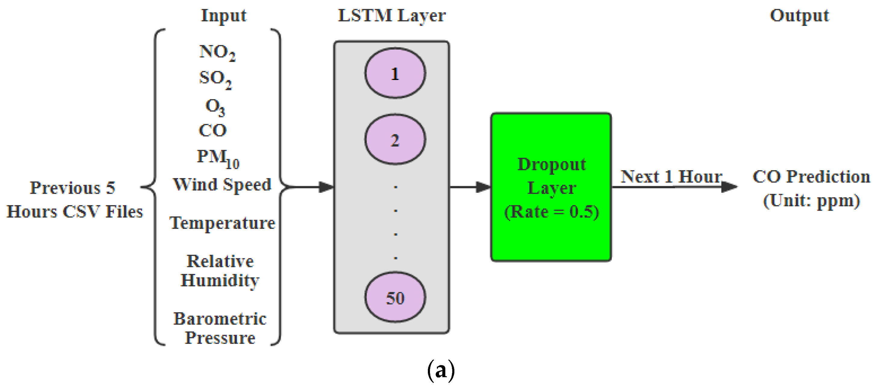
• LSTM: In this paper, the first step in model development would be to transform input data into an appropriate 3D format for LSTM. One of the advantages of using this model is that it retains the time aspect of data and helps identifying complex non-functional relationships between data compared to statistical models which only focus on linearity in data. In this paper, we went through various iterations of the fine-tuning model by changing LSTM units per layer, adding additional LSTM layers and selecting different features. We got best results for 5 past hours’ data with 50 LSTM layers for carbon monoxide and further tuned model to avoid overfitting by adding 11 regularizes and 0.5 dropout. We also did an early stop with a patience value of 20 to save the best model, shown in Figure 1a. Similar to $\mathrm{CO}$, a model for $O_3$ is developed with a dropout rate of 0.4. It had nine input features from the past 5 h.
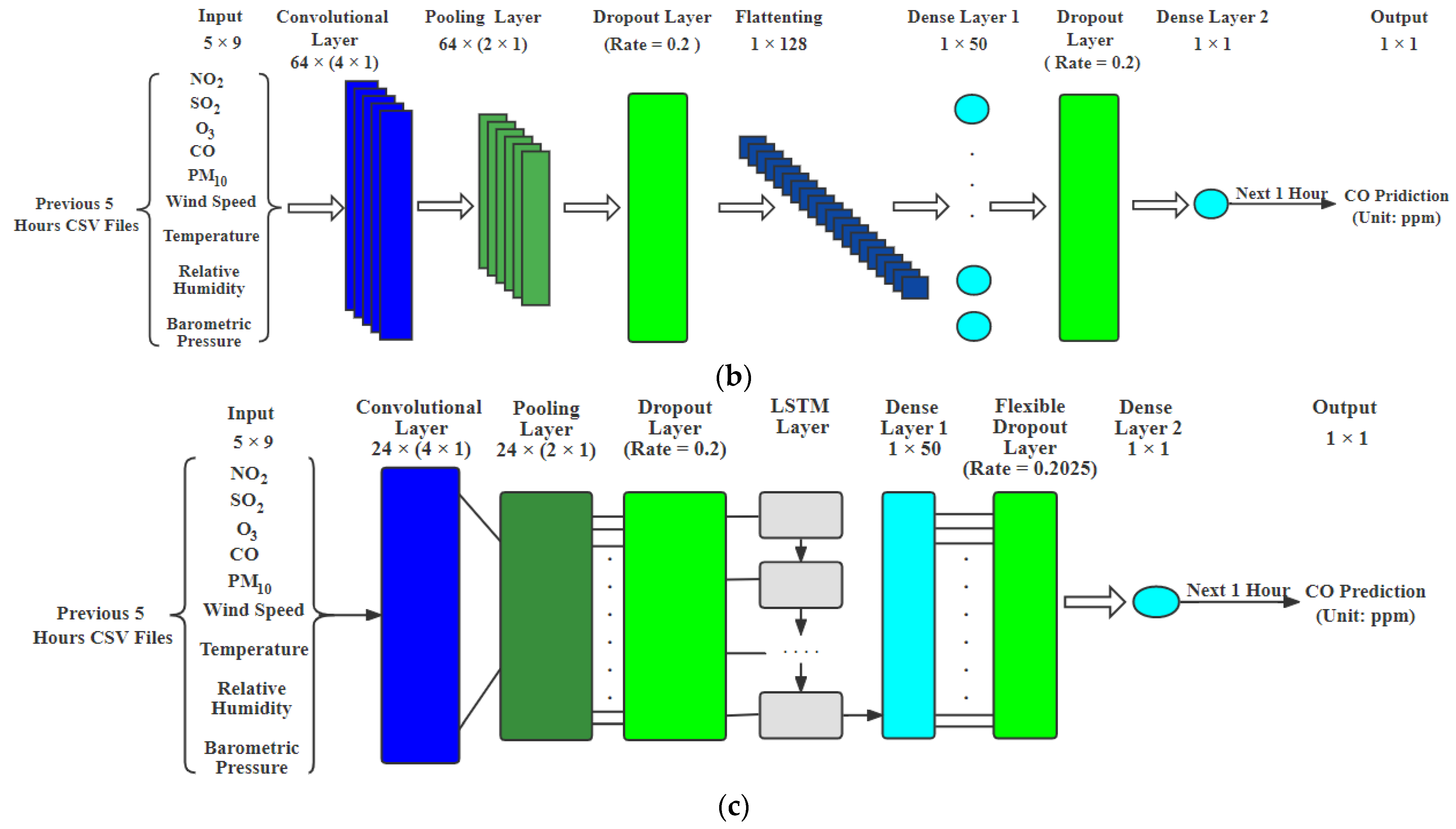
• CNN: In this paper, a one-dimensional CNN is used. We have one CNN layer followed by a pooling layer and then tune the number of hidden layers with “ReLU” activation and add a dropout layer if required. We only added a dropout layer after the pooling layer and the fully connected layer 1 for $\mathrm{CO}$ prediction. The final layer would have one output without any function. Figure 1b shows the CNN model architecture for hourly $\mathrm{CO}$ prediction.
• DFN: In this paper, the DFN model was employed to forecast air pollutants with our data, in which the LSTM layer includes 24 LSTM memory units. We removed the flexible dropout layer for ozone prediction. For $\mathrm{CO}$ prediction, we used the DFN model with a flexible dropout layer and the dropout rate can be obtained by $0.19+0.0025\times \mathrm{g}$ [26], which is 0.2025, in which the window size g was chosen as 5 h for our data, as shown in Figure 1c.

4.2. Hourly $P{M}_{2.5}$ and $P{M}_{10}$ Prediction

To perform the hourly forecasting of $P{M}_{2.5}$ and $P{M}_{10}$, we proposed an ensemble model, which is created by using a RF regressor and gradient boosting (GBoost) regressor. Models were individually optimized using the Bayes optimization method. This method uses the surrogate function and the concept of the Bayes theorem for tuning the hyperparameters of ML models. This method is efficient and fast for models with continuous and conditional parameters. In this paper, an ensemble model performs the weighted average of these two models for making final predictions. We assigned different weights to each model based on their individual scores. RF regressor with weight of 0.75 and GBoost regressor with weight 0.25 gave the best results. To predict the upcoming hour of $P{M}_{2.5}$ concentration in the air, the model is given 5 h of past concentrations of seven features, which are $P{M}_{2.5}$, $P{M}_{10}$, barometric pressure, dew point, wind speed, humidity and temperature, shown in Figure 2. Similar to $P{M}_{2.5}$, the model is given 5 h of past concentrations of seven features, which are $P{M}_{2.5}$, $P{M}_{10}$, $\mathrm{CO}$, $N{O}_2$, $O_3$, $S{O}_2$ and wind speed to predict the upcoming hour of $P{M}_{10}$ concentration in the air.

4.3. Daily Satellite-Based $P{M}_{2.5}$ and $P{M}_{10}$ Prediction

For the prediction of the $P{M}_{2.5}$ and $P{M}_{10}$ concentrations based on satellite data, we have developed three base models, which are the the RF, the SVR and XGBoost. To obtain a better performance, we created two ensemble models of the above three models, including a weighted average ensemble model and stacked ensemble, which were implemented for making the final prediction. To predict the daily $P{M}_{2.5}$ concentration in the air, each model is given the data of NDVI, distance to the Salton Sea, $P{M}_{2.5}$, $P{M}_{10}$, barometric pressure, dew point, wind speed, humidity and temperature as input. To predict daily $P{M}_{10}$ concentration in the air, each model is given data of NDVI, distance to the sea we studied, $P{M}_{2.5}$, $P{M}_{10}$, $\mathrm{CO}$, $N{O}_2$, $O_3$, $S{O}_2$ and wind speed as input. Except for inputs and model parameters, each model architecture for $P{M}_{10}$ prediction is similar to $P{M}_{2.5}$; therefore, we only show each model architecture for the $P{M}_{2.5}$.

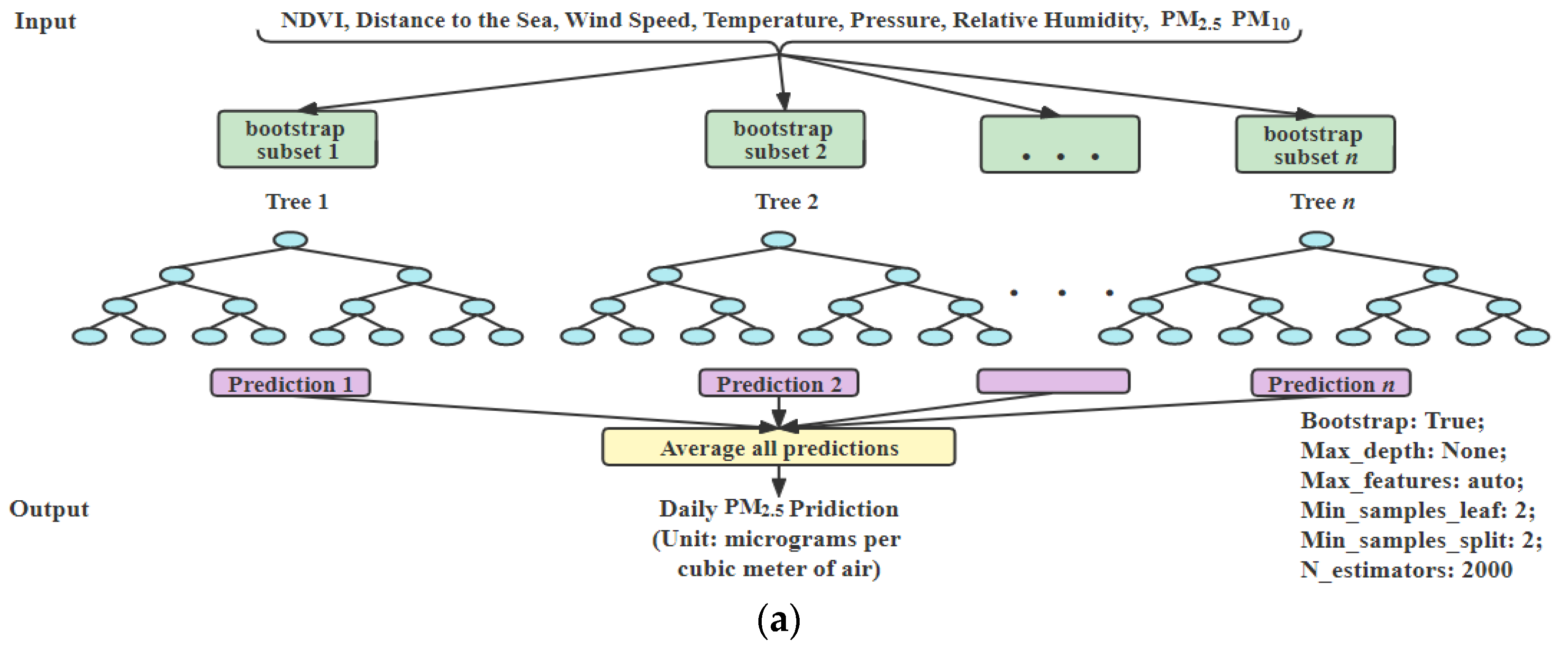
• RF: RF is a tree-based ensemble model. It is easy to use and has good performance on large data. We use Grid Search CV with threefold to optimize the parameters. RF model architecture for daily $P{M}_{2.5}$ prediction is shown in Figure 3a. The parameters of RF model are “bootstrap: true, max_depth: 50, max_features: auto, min_samples_leaf: 2, min_samples_split: 2, n_estimators: 500” for $P{M}_{10}$.
• SVR: SVR is very similar to support vector machines (SVM), which can be used in classification and clustering problems. While iterating SVR, we put a Grid Search CV of parameters, using threefold cross-validation, and search for different combinations in order to obtain the better result. We use SVM as our base model in the “PM concentration prediction using satellite images” part. The parameters of SVR model are “kernel = ‘rbf’, degree = 3, gamma = ‘auto’, C = 100” for $P{M}_{2.5}$, and “kernel = ‘rbf’, degree = 3, gamma = ‘scale’, C = 100” for $P{M}_{10}$.
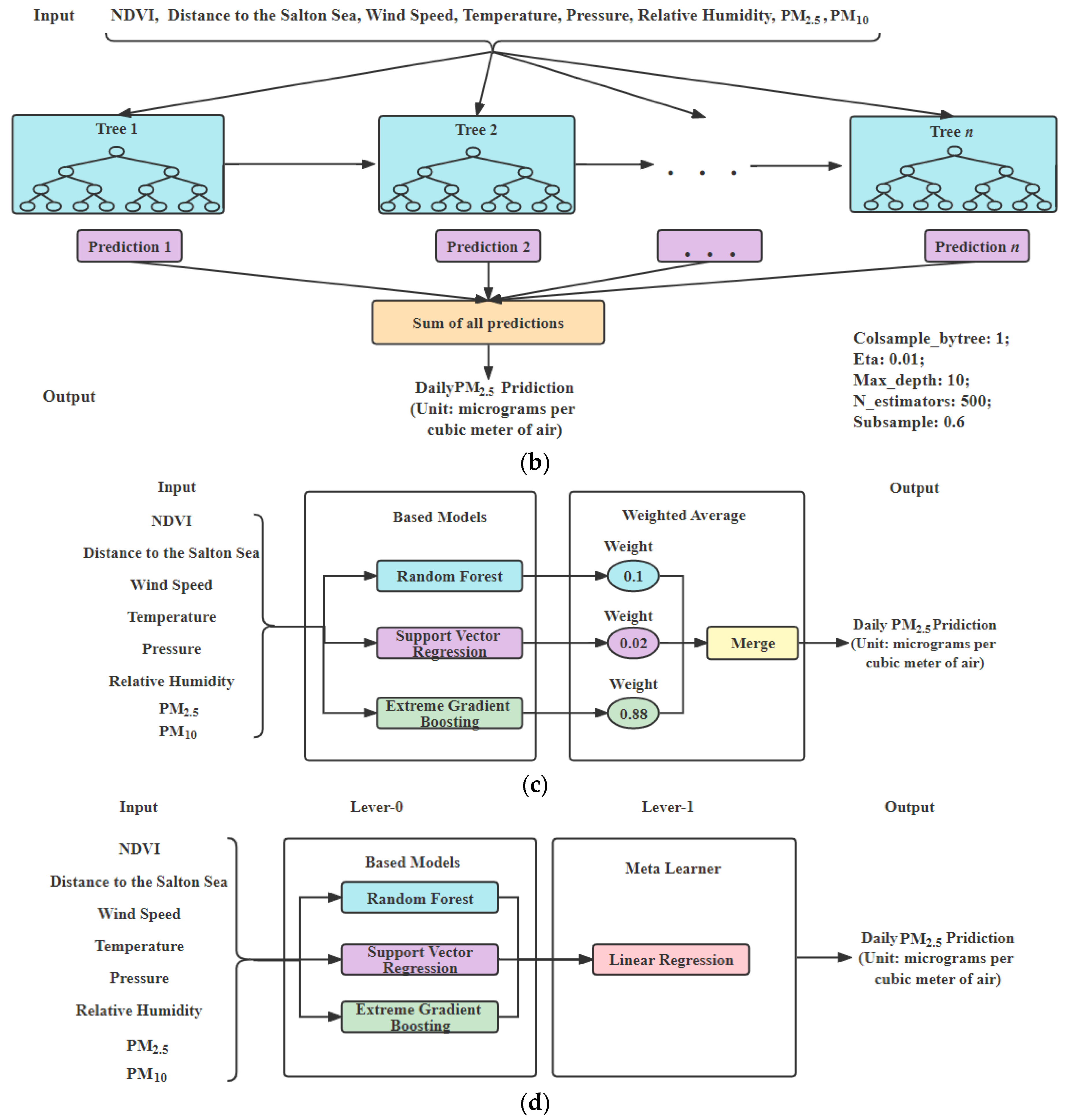
• XGBoost: XGBoost is simple, efficient and easy to implement, which is suitable for dealing with a large number of pulsar candidates with an excellent generalization performance. XGBoost model architecture for daily $P{M}_{2.5}$ prediction is shown in Figure 3b. The parameters of XGBoost model are “colsample_bytree: 1; eta: 0.01; max_depth: 10; n_estimators: 2500; subsample: 0.8” for $P{M}_{10}$.
• Weighted average ensemble model: The weighted average ensemble model is created by using SVR, RF and XGBoost for daily $P{M}_{2.5}$ prediction. Weights for RF, SVR and XGBoost are set to 0.1, 0.02, and 0.88, respectively, based on their individual performance, shown in Figure 3c.
• Stacked ensemble model: The stacked ensemble model is created by using SVR, RF and XGBoost, in which the base learners are SVR, RF and XGBoost and the meta learner is LR. The models of SVR, RF and XGBoost are used as Level-0 stage, and our meta learner LR is used as Level-1 in order to find target features for daily PM prediction. Figure 3d shows the stacked ensemble model with linear regression for daily $P{M}_{2.5}$ prediction.

4.4. Asthma Prevalence Rate Prediction

For health impact prediction, we used air pollutants data, weather data and asthma data to predict asthma prevalence rate among different ages. Starting with RF, GridSearch was used to finetune each model. The SVR was also included to obtain the lowest error rate, thus yielding a better fitting model. The third model, the elastic net regression (ENR) model, was employed to reduce overfitting problems in linear models and to eliminate coefficients about unimportant attributes. Since GBoost is one of the powerful algorithms in ML, which focuses on minimizing the bias error by combining several weak learners to form a strong learner. We tuned multiple parameters of GBoost and found the optimal n_estimators value, which is critical for asthma prediction. To obtain a better performance, we created two ensemble models of all four models as discussed above. Methods like weighted average and stacked ensemble are implemented for making the final prediction as follows. The input of each model is the data of $N{O}_2$, $S{O}_2$, $O_3$, $\mathrm{CO}$, $P{M}_{2.5}$, $P{M}_{10}$, wind speed, pressure, dew point, temperature, relative humidity and the healthy data. The output is the prediction of the ED asthma visits.

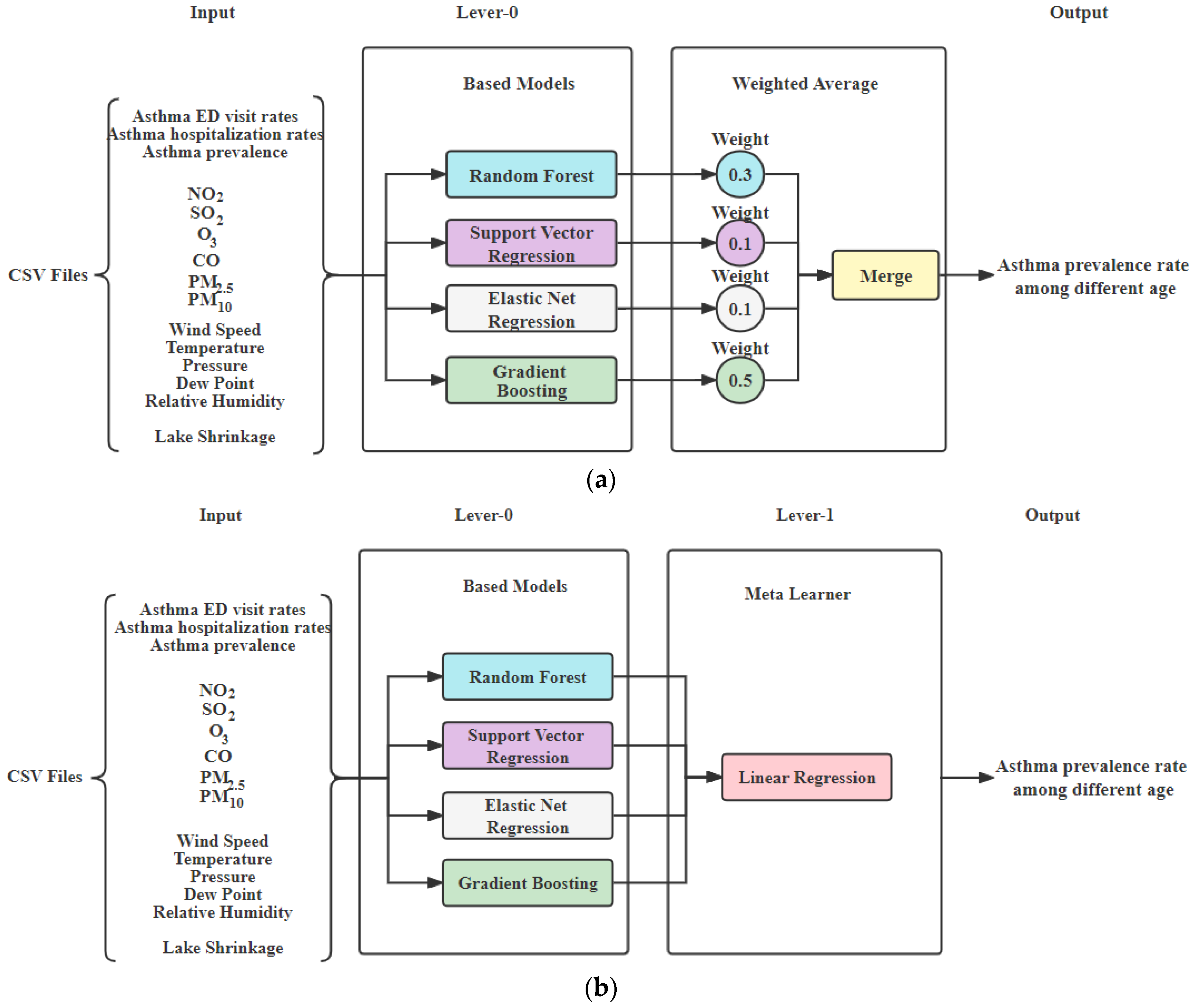
• Weighted average ensemble model: The weighted average ensemble model is created by using RF, SVR, ENR, and GBoost. Weights for RF, SVR, ENR, and GBoost are set to 0.3, 0.1, 0.1, 0.5, respectively, based on their individual performance, as shown in Figure 4a.
• Stacked ensemble model: The stacked ensemble model is created by using RF, SVR, ENR, and GBoost, in which the base learners are RF, SVR, ENR, and GBoost and the meta learner is LR. The models of RF, SVR, ENR, and GBoost are used as the Level-0 stage, and our Meta learner LR was used as Level-1 in order to find target features, as shown in Figure 4b.

5. Case Study Results

In this section, the Salton Sea, one of the largest lakes in California, is taken as an example to analysis the environmental pollution and study its impact on health. The water level is decreasing, and the special terrain makes the Salton Sea react poorly to pollution. Not only do factories dump industrial waste into it, but the low rainfall precipitation rate causes the Salton Sea to shrink. The proposed models are developed to forecast the air quality, dust emission due to shrinkage of the Salton Sea, and their impacts on human health as following.

5.1. Hourly Air Pollutant Prediction Results

We have developed models for each of the four pollutants, which are $O_3$, $\mathrm{CO}$, $P{M}_{2.5}$ and ${PM}_{10}$. These are the major pollutants impacting the Salton Sea area. These pollutants are directly correlated to dust and temperature in the region. Based on these pollutants, the final Air Quality Level (AQL) will be determined for the upcoming hour in the area. Air Quality Index (AQI) level will be based on the US EPA standards.

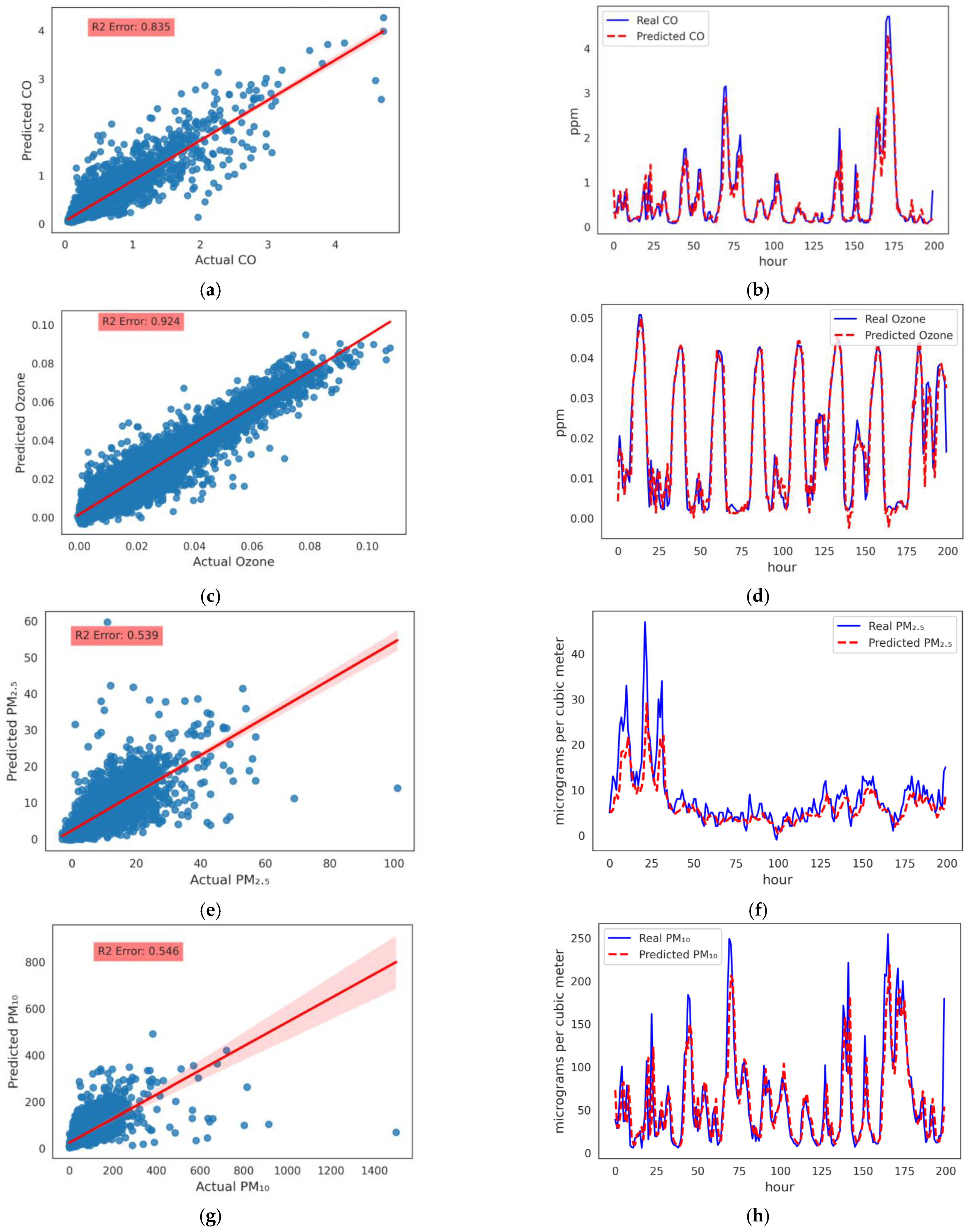
• Hourly $\mathrm{CO}$ and $O_3$ Prediction: Three proposed models, which are the LSTM, the CNN and the DFN, were developed and evaluated for predicting the upcoming hour $\mathrm{CO}$ and $O_3$ concentration. Models were trained for 100 epochs using the Adam optimizer and loss was evaluated using mean squared errors (MSE). Training of the LSTM model compared to the other two models seemed to be stable and learned better after 100 epochs, and the loss of both training and validation data is close to each other. The results comparison for the different models is shown in

  Table 5. Comparison of forecasting models evaluation results based on meteorological station data (created by author).

  Pollutant	Models	RMSE	MAE	R2
  CO	LSTM	0.151	0.075	0.835
  	CNN	0.175	0.106	0.779
  	DFN	0.187	0.115	0.747
  Ozone	LSTM	0.005	0.004	0.924
  	CNN	0.007	0.005	0.856
  	DFN	0.008	0.006	0.839
  PM2.5	RF	4.678	2.851	0.431
  	GBoost	4.231	2.502	0.535
  	Ensemble	4.212	2.504	0.539
  PM10	RF	37.754	16.612	0.548
  	GBoost	38.329	16.421	0.534
  	Ensemble	37.713	16.439	0.549

  . We obtained best results with LSTM for $\mathrm{CO}$ and $O_3$. Test data samples with predicted and actual values are shown in Figure 5a,c for $\mathrm{CO}$ and $O_3$, respectively. The line chart for predicted and actual $\mathrm{CO}$ and $O_3$ values is shown in Figure 5b,d for the LSTM model, respectively. Red dotted and blue lines for predicted and actual values of $\mathrm{CO}$ and $O_3$ in the test data are very close to each other for LSTM model. Comparison is drawn after re-scaling values to the original unit of data, i.e., ppm. Results in Figure 5 showed that there is a strong relationship between both the values and our model gave accurate results with very less errors.
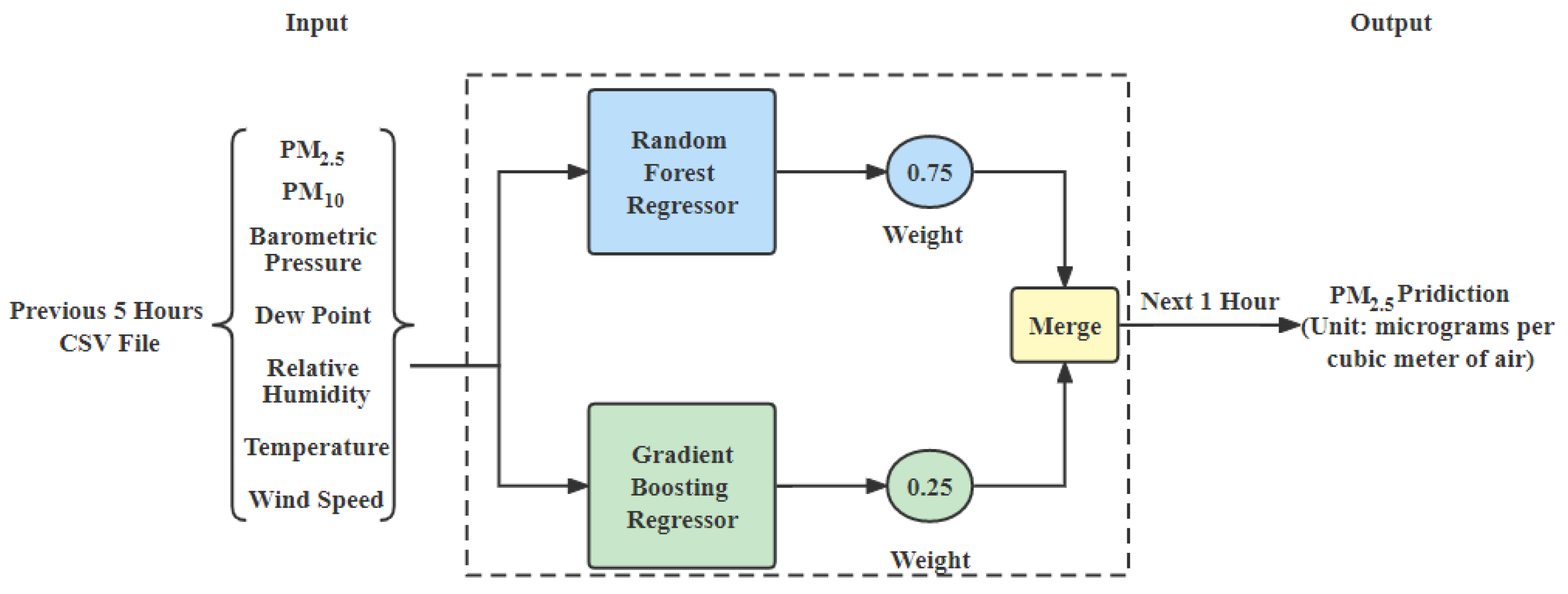
• Hourly PM Prediction Using Meteorological Station Data: ML models were developed and tuned. DL models are not able to provide the best results, and there is no training in using the DL models. We developed an ensemble model of RF and GBoost for ${\mathit{PM}}_{2.5}$ and ${\mathit{PM}}_{10}$ prediction. Test data samples with predicted and actual values are shown in Figure 5e,g for ${\mathit{PM}}_{2.5}$ and ${\mathit{PM}}_{10}$ respectively. Line chart for predicted and actual ${\mathit{PM}}_{2.5}$ and ${\mathit{PM}}_{10}$ values is shown in Figure 5f,h for the ensemble model of RF and GBoost, respectively. We can see in the results that the model has predicted results accurately. The proposed models in this paper have high capabilities and strengths over other models for our targeted problem.

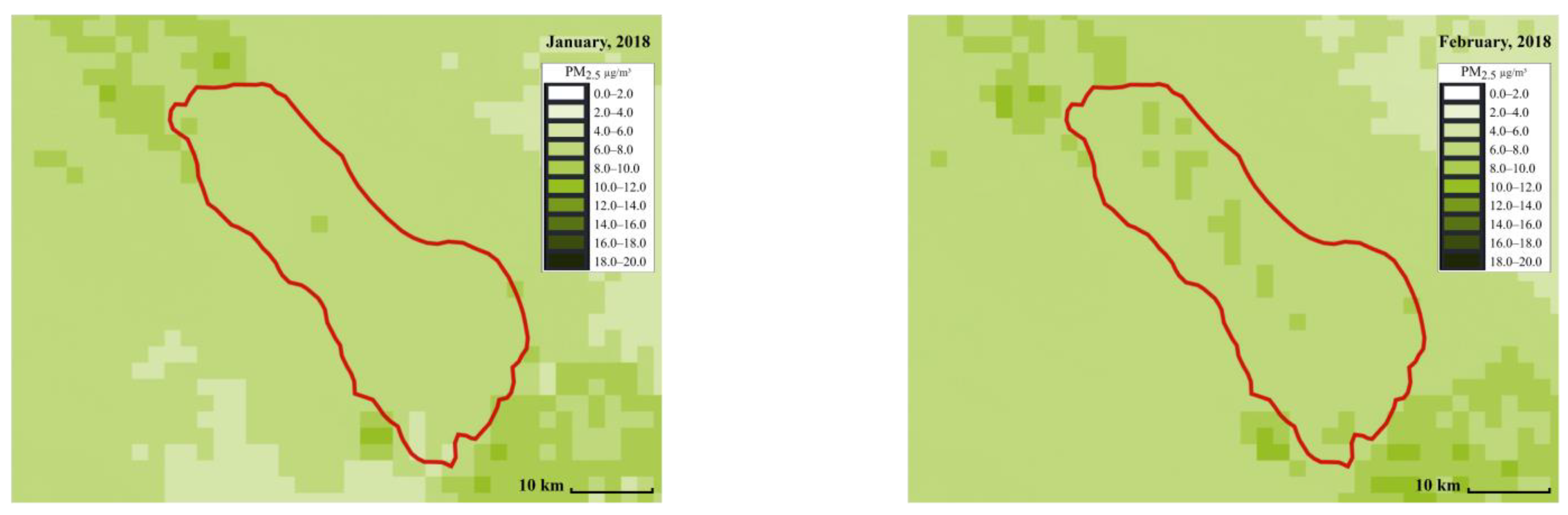
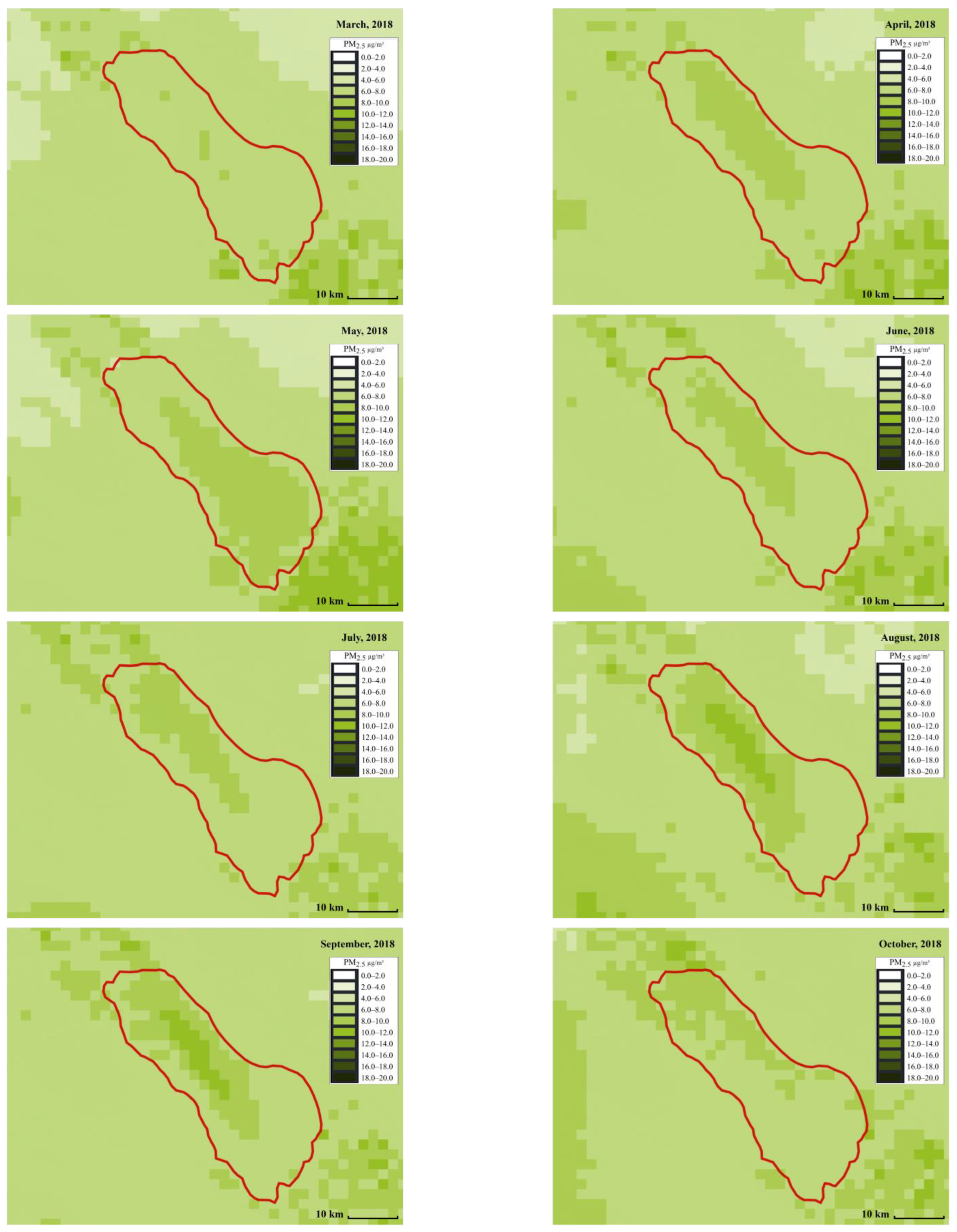
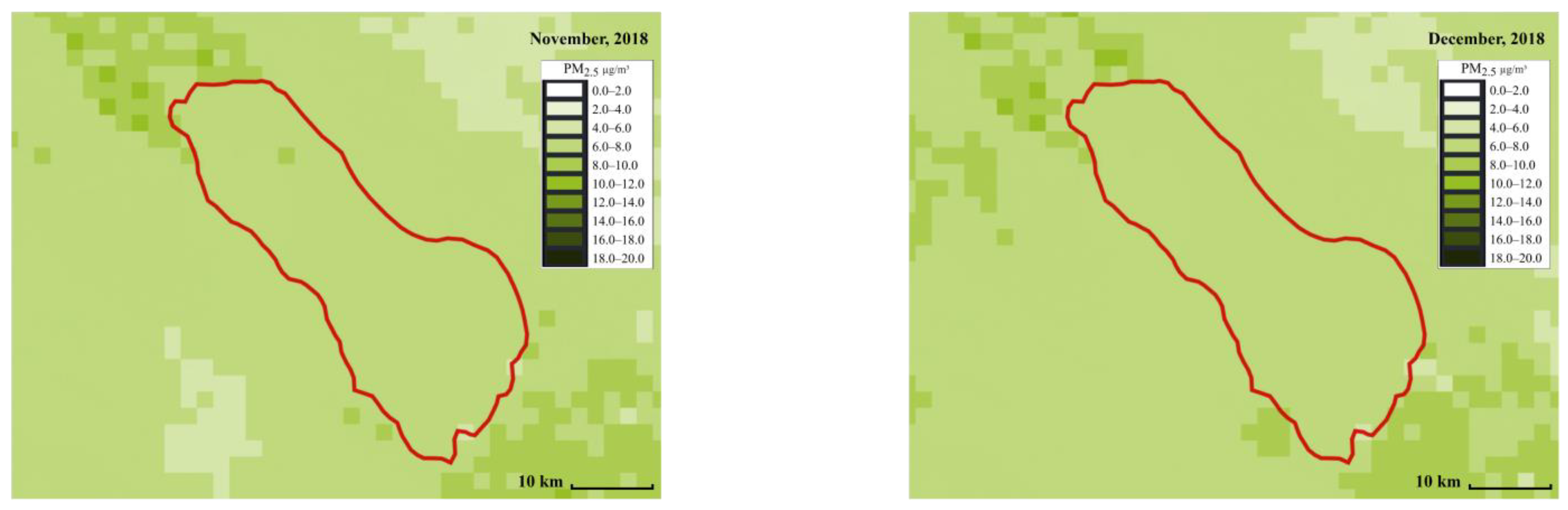
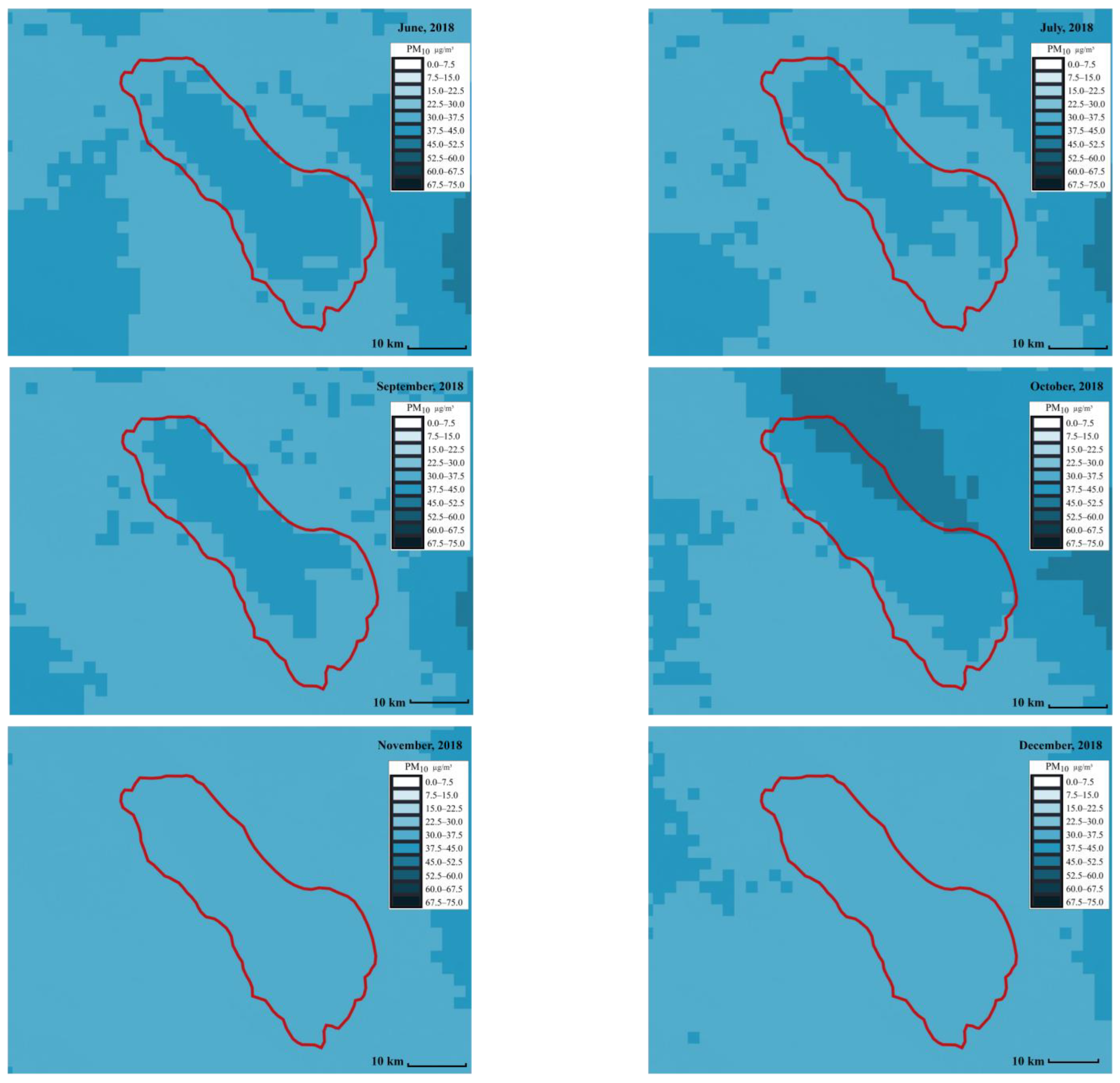
5.2. Satellite-Based Daily Particulate Matter Prediction Results

The PM data from the meteorological station only reflects the PM concentration around the station. As such, in order to explore the ${\mathit{PM}}_{2.5}$ and ${\mathit{PM}}_{10}$ situation around the Salton Sea area and show the temporal and spatial particulate matter change, RF, SVR, XGBoost were developed to explore the relationship between NDVI from the satellite data and ground-level PM concentration. Three proposed models were tuned using grid search.

Table 6. Comparison of forecasting models evaluation results based on satellite data (created by author).

Pollutant	Models	R2	RMSE	MAE
PM2.5	RF	0.71	3.38	2.35
	SVR	0.62	3.89	2.76
	XGBoost	0.75	3.14	2.58
	Weighted average	0.76	3.09	2.09
	Stacked ensemble	0.76	2.83	2.04
PM10	RF	0.68	12.97	8.08
	SVR	0.60	14.42	8.76
	XGBoost	0.74	11.69	7.11
	Weighted average	0.74	11.63	7.11
	Stacked ensemble	0.74	11.69	7.11

shows the performance of three base models of SVR, RF, XGBoost and the two ensemble models. For the ${\mathit{PM}}_{2.5}$ prediction, the stacked ensemble outperformed the other models with a good R2 score of 0.76. Hence, the stacked ensemble model is selected as a candidate model. For ${\mathit{PM}}_{10}$ prediction, the weighted average ensemble model has the highest accuracy. Additionally, we explored the stacked ensemble and weighted average ensemble methods to identify the best model for our research.

We focus on showing the daily PM concentration map in the Salton Sea area. As for the Salton Sea area, the expanding dry lakebed is a significant source of dust during the late spring to early summer [45]. Satellite-based ${\mathit{PM}}_{2.5}$ and ${\mathit{PM}}_{10}$ concentration maps were created to visualize the regions with the highest and lowest pollutants. Figure 6 and Figure 7 show the distribution of ${\mathit{PM}}_{2.5}$ and ${\mathit{PM}}_{10}$ across different months, respectively. The red line represents the Salton Sea area. Each small square in the figures represents an area of 2 km by 2 km. The darker the square, the higher the PM concentration. The PM concentration around the Salton Sea and its surroundings can be intuitively displayed in the form of snapshots using ML at different times and places, making it more convenient for people to compare and analyze the PM concentration. From the comparison, we can see that spring (from March to May), and summer (from June to August) have the highest concentrations. This can be due to the fact that wind speed is high around this time.

5.3. Health Impact Prediction Results

Four models, RF, SVR, ENR, and GBoost, were developed to predict the asthma prevalence in both counties of the Salton Sea. We conducted hyperparameter tuning for all the estimators using Gridsearch () with a cv = 5. The best parameters given by the GridSearchCV are used as the estimators for training. Additionally, we explored the weighted average ensemble model and stacked ensemble method to identify the best model for our research. Weights for RF, SVR, ENR, and GBoost were set to 0.3, 0.1, 0.1, 0.5, respectively, based on their individual performance. The weighted average model has a good R2 score of 0.95. We further attempted to improve the model performance by creating a stacked ensemble model. Here, the base learners are RF, SVR, ENR, GBoost, and the meta learner is LR. The stacked ensemble outperformed the other models with a good R2 score of 0.978. Hence, the stacked ensemble is selected as a candidate model for predicting the health impact.

Table 7. Comparison of Models for Asthma Prediction (created by author).

Models	Model Set Parameter	R2	MAE	MSE	RMSE
RF	Criterion = ‘mse’, max_depth = 50, n_estimators = 100, max_features = 20, random_state = 42.	0.945	0.026	0.002	0.045
SVR	Kernel = ‘rbf’, gamma = ‘auto’, C = 100, epsilon = 0.01.	0.897	0.038	0.003	0.062
ENR	Alpha = 0.0001,11_ratio = 0.5, max_iter = 1000, normalize = True.	0.753	0.068	0.009	0.097
GBoost	max_depth = 50, max_features = 20, min_samples_leaf = 10, min_samples_split = 50, n_estimators = 100, random_state = 42.	0.949	0.024	0.001	0.043
Weighted Average	Weights for RF, SVR, ENR and GBoost are set to 0.3, 0.1, 0.1, 0.5.	0.95	0.026	0.001	0.043
Stacked Ensemble	Base learners: RF, SVR, ENR, GBoost. Meta learner: LR.	0.978	0.021	0.001	0.037

shows the results of the comparison of all the models.

6. Discussion

6.1. Comparison of Hourly Air Pollutant Forecasting Models

Table 8. Comparison of forecasting models of air pollutants (created by author).

Papers	Region	Purpose	Model	Accuracy	Input Parameters
[22]	Shanghai, China	$\mathrm{Predicting}P{M}_{2.5}$	Ensemble Model 1	MAE: 6.19 MAPE: 0.162	$P{M}_{2.5}$, meteorological data, season data, timestamp data
[23]	Kuwait	Forecasting ozone	LSTM	MAE < 2	Hourly air quality, meteorological data
[24]	Taiwan	Predicting hourly air quality	CNN	RMSE: 7.37	$\mathrm{Hourly}\mathrm{ozone},\mathrm{particulate}\mathrm{matter}P{M}_{2.5}$ and sulfur dioxide
[25]	Seoul, South Korea	Predicting ozone	CNN	MAE: 8.90	Ground-level ozone and ${NO}_2$, atmospheric pressure, wind speeds and relative humidity
[26]	Aksaray, AlibeyköyBeşiktaş, Esenler, Istanbul	$\mathrm{Forecasting}P{M}_{10}$ in upcoming hours	DFN	RMSE: 13.67	$P{M}_{10}$ density, meteorological data pollution data, traffic data
This work	California, USA	$\mathrm{Predicting}{O}_3$ in upcoming hour	LSTM	MAE: 0.004 RMSE: 0.005 R2: 0.924	Air pollutants, meteorological parameters
This work	California, USA	$\mathrm{Predicting}\mathrm{CO}$ in upcoming hour	LSTM	MAE: 0.075 RMSE: 0.151 R2: 0.835	Air pollutants, meteorological parameters
This work	California, USA	$\mathrm{Predicting}P{M}_{2.5}$ in upcoming hour	Ensemble Model 2	MAE: 2.504 RMSE: 4.212 R2: 0.539	$P{M}_{2.5}$$,P{M}_{10}$, air pressure, dew point, wind speed, humidity, and temperature
This work	California, USA	$\mathrm{Predicting}P{M}_{10}$ in upcoming hour	Ensemble Model 2	MAE: 16.439 RMSE: 37.713 R2: 0.549	$P{M}_{2.5}$$,P{M}_{10}$$,\mathrm{CO}$$,N{O}_2$$,O_3$$,S{O}_2$ and wind speed

Abbreviations: Ensemble Model 1 (ensemble model of RNN, LSTM, and GRU); Ensemble Model 2 (weighted average ensemble model of RF and GBoost).

shows the performance of these selected models in various research with time series data for air quality forecasting. We can see that the DL models tend to perform better by identifying even nonlinear relationships in time steps. The proposed models in this paper have high capabilities and strengths over other models for our targeted problem. Additionally, with these models, it is easier to implement and evaluate multivariate time series for forecasting even multiple time steps if required.

Once we predicted the individual pollutants, we calculated the overall air quality index for that hour and compared original and predicted AQI values.

Table 9. Comparison of Original and Predicted AQI Results (created by author).

	Original AQI Level	Predicted AQI Level
Good	1719	1758
Moderate	426	393
Unhealthy for Sensitive Groups	9	4
Unhealthy	1	Not Available

shows the comparison of original and predicted AQI results. The final accuracy for the AQI level is 86.7%.

6.2. Comparison of Satellite-Based Daily Particulate Matter Forecasting Models

Table 10. Comparison between the models for forecasting particulate matter based on satellite data (created by author).

Papers	Region	Purpose	Model	Accuracy	Input Parameters
[17]	Quito, Ecuador	$\mathrm{Predicting}\mathrm{daily}P{M}_{10}$	MLP	R2: 0.68	Surface reflectance bands of Landsat-8, NDVI, NDSI, SAVI, NDWI, LST
[18]	Chile	$\mathrm{Predicting}\mathrm{daily}P{M}_{10}$	MLP	R2: 0.58	AOD, meteorological variables
[19]	Alberta, Canada	$\mathrm{Predicting}\mathrm{daily}P{M}_{10}$	MLP	R2: 0.61	AOD, meteorological variables
[20]	Malaysia	$\mathrm{Predicting}\mathrm{daily}P{M}_{2.5}$	MLP	R2: 0.60	AOD, meteorological and spatial variables
[21]	Tehran, Iran	$\mathrm{Predicting}\mathrm{daily}P{M}_{2.5}$	RF	R2: 0.81 MAE: 9.93 RMSE: 13.58	Satellite image, meteorological variables
This work	California, USA	$\mathrm{Predicting}\mathrm{daily}P{M}_{2.5}$	Ensemble Model 3	MAE: 2.04 RMSE: 2.83 R2: 0.76	MODIS based NDVI, Landsat 8 based distance to the Salton Sea, weather, air pollutants
This work	California, USA	$\mathrm{Predicting}\mathrm{daily}P{M}_{10}$	Ensemble Model 4	MAE: 7.11 RMSE: 11.63 R2: 0.74	MODIS based NDVI, Landsat 8 based distance to the Salton Sea, weather, air pollutants

Abbreviations: Ensemble Model 3 (weighted average ensemble model of RFR, SVR, and XGBoost), Ensemble Model 4 (stacked ensemble model of RF, SVR, XGBoost and LR).

shows the performance of the recently proposed models in various research with satellite data and other variables as the input for particulate matter forecasting. For the $P{M}_{2.5}$ prediction, the proposed weighted average ensemble model of RFR, SVR, and XGB outperformed most of the other models with a good R2 score of 0.76. For $P{M}_{10}$ prediction, the proposed stacked ensemble model of RF, SVR, XGBoost and LR has the highest accuracy among all of the other models.

6.3. Comparison of Health Impact Forecasting Models

Table 11. Comparison of Health Prediction Models (created by author).

Papers	Region	Purpose	Model	Accuracy	Input Parameters
[27]	United States	Identifying the impact of pollution on the behavior of people	RF	NRMSE: 0.0798	$\mathrm{Indoor}\mathrm{Air}\mathrm{quality},O_3$$,\mathrm{SOX}$$,\mathit{PM}$, Volatile Organic Compounds
			LR	NRMSE: 0.2259
			SVR	NRMSE: 0.2591
[28]	Tehran, Iran	Studying asthma based on environmental factors along with map locations	RF	Training AUC: 0.987 Testing AUC: 0.921	$P{M}_{2.5}$$,P{M}_{10}$$,\mathrm{CO}$$,N{O}_2$$,\mathrm{SO}$$,O_3$, wind speed, rainfall, humidity and temperature
[29]	Seoul, South Korea	Predicting the number of asthma patients at daily level	VAR	MAE: 668.50	$S{O}_2$$,\mathrm{CO}$$,O_3$$,N{O}_2$$,P{M}_{2.5}$$,P{M}_{10}$, humidity, temperature, air pressure
			HDLM	MAE: 479.31
			DFNN	MAE: 691.22
			LSTM	MAE: 821.72
[30]	California, United States	Showing the correlation between daily air quality and asthma patients	Ridge	RMSE: 0.042	Daily air quality
			EN	RMSE: 0.0413
			LASSO	RMSE: 0.0412
			Gamboost	RMSE: 0.039
			DT	RMSE: 0.026
			RF	RMSE: 0.71
[31]	Seoul, South Korea	Predicting chances of asthma on children because of inside air pollution	MNL	LSTM outperformed MNL by 57–84% increase in precision	Temperature and particulate matter for indoors (for 10 min internal)
			LSTM
This work	California, United States	Predicting the asthma prevalence rate	Ensemble Model 5	MAE: 0.021 MSE: 0.001 RMSE: 0.037 R2: 0.976	$N{O}_2$$,S{O}_2$$,O_3$$,\mathrm{CO}$$,P{M}_{2.5}$$,P{M}_{10}$, wind speed, pressure, dew point, temperature, relative humidity, healthy data

Abbreviation: Ensemble Model 5 (stacked ensemble of RF, SVR, ENR, GBoost and LR).

shows the performance of the recently proposed models in various research with air quality and other variables as the input for health prediction. We can see that the proposed stacked ensemble model of RF, SVR, ENR, GBoost and LR in this paper outperformed the other models with a good R2 score of 0.978.

7. Conclusions

In this paper, we have proposed forecasting models to predict the health impacts caused by the air quality in the Salton Sea, which have been divided into three main parts, the environmental air pollutants, particulate matter and the asthma ED visits, respectively. Each model performed relatively well. Firstly, for hourly air pollutant forecasting, the LSTM model was deployed on both $O_3$ and $\mathrm{CO}$ forecasting by using the previous 5 h of all pollutants and weather conditions. The MSE loss function and Adam optimizer were employed to evaluate the performance, and the results showed that the LSTM model obtained the best results due to low error. Secondly, as for hourly $P{M}_{2.5}$ and PM₁₀ prediction, the ensemble model of weighted average method based on RF and GBoost are proposed by using the previous 5 h of air pollutants and weather conditions. The models are tuned by implementing Bayes optimization to obtain the best result. We can achieve a 0.9 score for ozone prediction. Then, for particulate matter prediction, the proposed ensemble model of weighted average method obtained the best result for predicting daily $P{M}_{2.5}$, and daily $P{M}_{10}$ has the best result while using the stacked ensemble model by comparing R2, RMSE and MAE values. Finally, for the health impact study, we used the SVR, ENR, RF and GBoost models on asthma ED visits prediction, in which the stacked ensemble was selected as a candidate model by comparison with the weighted average method with a good R2 score of 0.978.

We have two goals for future work. Above all, we can enhance our satellite data by incorporating more satellites in future. Our specific goal is to collect data from other satellites and make a finer prediction of PM concentration around the Salton Sea. In addition, our broad goal is to develop real-time health impact prediction dashboards to highlight the relationship between various environmental factors and asthma prevalence rates for more cities around the Salton Sea in the future.

References

- Fendt, L. As the Salton Sea Shrinks, It Leaves behind a toxic reminder of the cost of making a desert bloom. Available online: https://thefern.org/2020/01/as-the-salton-sea-shrinks-it-leaves-behind-a-toxic-reminder-of-the-cost-of-making-a-desert-bloom/ (accessed on 10 December 2021).
- Baj, A.; Jf, B. Shrinking lakes, air pollution, and human health: Evidence from California’s Salton Sea. Sci. Total Environ. 2020, 712, 136490. [Google Scholar] [CrossRef]
- Zelenko, M. Dust Rising. 2018. Available online: https://www.theverge.com/2018/6/6/17433294/salton-sea-crisis-drying-up-asthma-toxic-dust-pictures (accessed on 20 February 2021).
- Gao, J.; Deo, A.; Chiao, S. Soil Evaluation Research for Salton Sea-A Survey of Available Salton Sea Soil and Sediment Evaluation Research Literature. J. Agric. For. Meteorol. Res. 2021, 4, 447–458. [Google Scholar]
- Chawla, P.; Cao, X.; Fu, Y.; Hu, C.-M.; Wang, M.; Wang, S.; Gao, J.Z. Water quality prediction of Salton Sea using machine learning and big data techniques. Int. J. Environ. Anal. Chem. 2021, 8, 1–24. [Google Scholar] [CrossRef]
- James, I. Salton Sea: Dusty Air and the Asthma Crisis at the Salton Sea. Available online: https://www.usatoday.com/pages/interactives/salton-sea/toxic-dust-and-asthma-plague-salton-sea-communities/ (accessed on 10 December 2021).
- Cooper, M. Imperial County Residents Help Tackle Air Monitoring. Available online: https://www.fondriest.com/news/imperial-county-residents-help-tackle-air-monitoring.htm (accessed on 10 December 2021).
- DeLara, J. Valley Voice: Fighting to Inhale-a Community Case at the Salton Sea. Available online: https://www.desertsun.com/story/opinion/contributors/valley-voice/2020/09/04/fighting-inhale-community-case-salton-sea-juan-delara-valley-voice/5710409002/ (accessed on 10 December 2021).
- Gholami, H.; Mohamadifar, A.; Sorooshian, A.; Jansen, J.D. Machine-learning algorithms for predicting land susceptibility to dust emissions: The case of the Jazmurian Basin, Iran. Atmos. Pollut. Res. 2020, 11, 1303–1315. [Google Scholar] [CrossRef]
- Bozdağ, A.; Dokuz, Y.; Gökçek, Ö.B. Spatial prediction of PM10 concentration using machine learning algorithms in Ankara, Turkey. Environ. Pollut. 2020, 263, 114635. [Google Scholar] [CrossRef] [PubMed]
- Fan, J.; Li, Q.; Hou, J.; Feng, X.; Karimian, H.; Lin, S. A spatiotemporal prediction framework for air pollution based on deep RNN. ISPRS Ann. Photogramm. Remote Sens. Spatial Inf. Sci. 2017, IV-4/W2, 15–22. [Google Scholar] [CrossRef] [Green Version]
- Azid, A.; Juahir, H.; Toriman, M.E.; Kamarudin, M.K.A.; Saudi, A.S.M.; Hasnam, C.N.C.; Aziz, N.A.A.; Azaman, F.; Latif, M.T.; Zainuddin, S.F.M.; et al. Prediction of the level of air pollution using principal component analysis and artificial neural network techniques: A case study in Malaysia. Water Air Soil Pollut. 2014, 225, 2063. [Google Scholar] [CrossRef]
- Li, X.; Peng, L.; Hu, Y.; Shao, J.; Chi, T. Deep learning architecture for air quality predictions. Environ. Sci. Pollut. Res. 2016, 23, 22408–22417. [Google Scholar] [CrossRef]
- Silas, M.; Dimitris, P.; Adrianos, R.; Filippos, T. Monitoring and forecasting air pollution levels by exploiting satellite, ground-based, and synoptic data, elaborated with regression models. Adv. Meteorol. 2017, 2017, 1–17. [Google Scholar]
- Stafoggia, M.; Bellander, T.; Bucci, S.; Davoli, M.; De Hoogh, K.; De Donato, F.; Gariazzo, C.; Lyapustin, A.; Michelozzi, P.; Renzi, M.; et al. Estimation of daily PM10 and PM2.5 concentrations in Italy, 2013–2015, using a spatiotemporal land-use random-forest model. Environ. Int. 2019, 124, 170–179. [Google Scholar] [CrossRef]
- Abdullah, S.; Ismail, M.; Najah, A.M. Multi-Layer Perceptron Model for Air Quality Prediction. Malays. J. Math. Sci. 2019, 13, 85–95. [Google Scholar]
- Vivanco, V. Assessment of remote sensing data to model PM10 estimation in cities with a low number of air quality stations: A case of study in quito, Ecuador. Environments 2019, 6, 85. [Google Scholar] [CrossRef] [Green Version]
- Yang, Z.; Hsu, K.; Sorooshian, S.; Xu, X.; Braithwaite, D.; Zhang, Y.; Verbist, K.M.J. Merging high-resolution satellite-based precipitation fields and point-scale rain gauge measurements-a case study in chile. J. Geophys. Res. Atmos. 2017, 122, 5267–5284. [Google Scholar] [CrossRef]
- Mirzaei, M.; Bertazzon, S.; Couloigner, I.; Farjad, B. Assessing the potential of artificial intelligence (artificial neural networks) in predicting the spatiotemporal pattern of wildfire-generated PM2.5 concentration. Geomatics 2021, 1, 3. [Google Scholar] [CrossRef]
- Zaman, N.; Kanniah, K.D.; Kaskaoutis, D.G. Satellite data for upscalling urban air pollution in malaysia. IOP Conf. Ser. Earth Environ. Sci. 2018, 169, 012036. [Google Scholar] [CrossRef]
- Joharestani, M.Z.; Cao, C.; Ni, X.; Bashir, B.; Talebiesfandarani, S. PM2.5 prediction based on random forest, xgboost, and deep learning using multisource remote sensing data. Atmosphere 2019, 10, 373. [Google Scholar] [CrossRef] [Green Version]
- Guo, C.; Liu, C.; Chen, C. Air Pollution Concentration Forecast Method Based on the Deep Ensemble Neural Network. Wirel. Commun. Mob. Comput. 2020, 8854649, 1–13. [Google Scholar] [CrossRef]
- Freeman, B.S.; Taylor, G.; Gharabaghi, B.; Thé, J. Forecasting air quality time series using deep learning. J. Air Waste Manag. Assoc. 2017, 68, 866–886. [Google Scholar] [CrossRef]
- Mao, Y.; Lee, S. Deep Convolutional Neural Network for Air Quality Prediction. J. Phys. Conf. Ser. 2019, 1302, 032046. [Google Scholar] [CrossRef]
- Eslami, E.; Choi, Y.; Lops, Y.; Sayeed, A. A real-time hourly ozone prediction system using deep convolutional neural network. Neural Comput. Appl. 2020, 32, 8783–8797. [Google Scholar] [CrossRef] [Green Version]
- Kaya, K.; Üdücü, S.G. Deep flexible sequential (DFS) model for air pollution forecasting. Sci. Rep. 2020, 10, 3346. [Google Scholar] [CrossRef] [PubMed]
- Lin, B.; Huangfu, Y.; Lima, N.; Jobson, B.; Kirk, M.; O’Keeffe, P.; Pressley, S.N.; Walden, V.; Lamb, B.; Cook, D.J. Analyzing the relationship between human behavior and indoor air quality. J. Sens. Actuator Netw. 2017, 6, 13. [Google Scholar] [CrossRef] [Green Version]
- Razavi-Termeh, S.V.; Sadeghi-Niaraki, A.; Choi, S.M. Asthma-prone areas modeling using a machine learning model. Sci. Rep. 2021, 11, 1912. [Google Scholar] [CrossRef] [PubMed]
- Kim, M.; Lee, J.; Jang, Y.; Lee, C.-H.; Choi, J.-H.; Sung, T.-E. Hybrid deep learning algorithm with open innovation perspective: A prediction model of asthmatic occurrence. Sustainability 2020, 12, 6143. [Google Scholar] [CrossRef]
- Chavda, J. Analyzing the Relationship between Asthma and Air Impurity in Developed Cities Using Machine Learning Approach. 2019. Available online: https://www.researchgate.net/publication/340949675 (accessed on 10 December 2021).
- Kim, D.; Cho, S.; Tamil, L.; Song, D.J.; Seo, S. Predicting asthma attacks: Effects of indoor PM concentrations on peak expiratory flow rates of asthmatic children. IEEE Access 2020, 8, 8791–8797. [Google Scholar] [CrossRef]
- Capan, M.; Hoover, S.; Jackson, E.; Paul, D.; Locke, R.; Capan, M. Time series analysis for forecasting hospital census: Application to the neonatal intensive care unit. Appl. Clin. Inform. 2016, 7, 275–289. [Google Scholar] [CrossRef] [Green Version]
- Air Quality Data Query Tool (AQDQT). 2021. Available online: https://www.arb.ca.gov/aqmis2/aqdselect.php (accessed on 10 December 2021).
- Meteorology Data Query Tool (MDQT). 2021. Available online: https://www.arb.ca.gov/aqmis2/metselect.php (accessed on 10 December 2021).
- NASA. 2021; MODIS Web. Available online: https://modis.gsfc.nasa.gov/about/ (accessed on 10 December 2021).
- Google. Landsat Data | Cloud Storage | Google Cloud. 2021. Available online: https://cloud.google.com/storage/docs/public-datasets/landsat (accessed on 10 December 2021).
- Environmental Protection Agency (EPA). 2021. Available online: http://www.epa.gov/pm-pollution/particulate-matter-pm-basics#effects (accessed on 10 December 2021).
- Asthma Emergency Department Visit Rates. California Health and Human Services Open Data Portal. 2018. Available online: https://data.chhs.ca.gov/dataset/asthma-emergency-department-visit-rates (accessed on 10 December 2021).
- Asthma Hospitalization Rates by County. California Health and Human Services Open Data Portal. 2018. Available online: https://data.chhs.ca.gov/dataset/asthma-hospitalization-rates-by-county (accessed on 10 December 2021).
- California Health and Human Services Open Data Portal. 2019. Available online: https://data.chhs.ca.gov/dataset/asthma-prevalence (accessed on 10 December 2021).
- Environmental Protection Agency (EPA). Available online: http://www.epa.gov/outdoor-air-quality-data/air-data-basic-information (accessed on 10 December 2021).
- California Air Resources Board (ARB). 2018. Available online: https://ww2.arb.ca.gov/our-work/topics/air-quality-monitoring#background (accessed on 10 December 2020).
- Database for Hydrological Time Series of Inland Waters (DAHITI). 2021. Available online: https://dahiti.dgfi.tum.de/en/ (accessed on 10 December 2020).
- Cordeiro, M.C.R.; Martinez, J.-M.; Peña-Luque, S. Automatic water detection from multidimensional hierarchical clustering for sentinel-2 images and a comparison with level 2A processors. Remote Sens. Environ. 2021, 253, 112209. [Google Scholar] [CrossRef]
- Frie, A.L.; Garrison, A.C.; Schaefer, M.V.; Bates, S.M.; Botthoff, J.; Maltz, M.; Ying, S.C.; Lyons, T.W.; Allen, M.F.; Aronson, E. Dust sources in the Salton Sea Basin: A clear case of an anthropogenically impacted dust budget. Environ. Sci. Technol. 2019, 53, 9378–9388. [Google Scholar] [CrossRef]