Abstract
Air pollution is one of the most pressing modern-day issues in cities around the world. However, most cities have adopted air quality measurement devices that only measure the past pollution levels without paying attention to the influencing factors. To obtain preliminary pollution information with regard to environmental factors, we developed a variational autoencoder and feedforward neural network-based embedded generative model to examine the relationship between air quality and the effects of environmental factors. In the model, actual , , , , and measurements from 2016 to 2020 were used, which were assembled from 15 differently located ground monitoring stations in Ulaanbaatar city. A wide range of weather and fuel measurements were used as the data for the influencing factors, and were collected over the same period as the air pollution data were recorded. The prediction results concerned all measurement stations, and the results were visualized as a spatial–temporal distribution of pollution and the performance of individual stations. A cross-validated was used to estimate the entire pollution distribution through the regions as : 0.81, : 0.76, : 0.89, and : 0.83. Pearson’s chi-squared tests were used for assessing each measurement station, and the contingency tables represent a high correlation between the actual and model results. The model can be applied to perform specific analysis of the interdependencies between pollution and environmental factors, and the performance of the model improves with long-range data.
1. Introduction
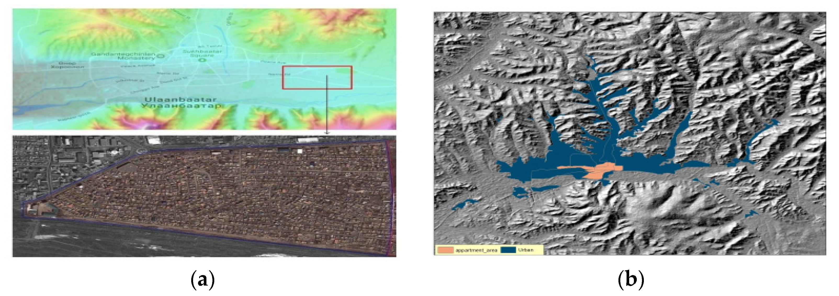
Serious environmental issues are common in densely populated large cities in developing countries. There are many factors contributing to this, starting with climate change; however, urbanization is a global problem [1]. In the past two decades, the number of inhabitants in Ulaanbaatar city has increased more than three times. The capital city of Mongolia sits on the Tuul River, the third-longest river in Mongolia, in a valley surrounded by large mountains, the geographical map of which is shown in Figure 1a. As the city was built in large river watershed lowland between mountains, the temperature is often inverse during the wintertime [2]. Moreover, the city’s geographical and climate features, as well as its poor heating system infrastructure, make the city one of the most air-polluted cities in the world today. The standard sewerage and pure water supply systems were initially designed for 400,000 inhabitants 46 years ago, but now around one 1.4 million people live in Ulaanbaatar, [3]. Some of these 1.4 million citizens are living in the boundary areas of the city, called ger districts in some reports, which are suburbs that are not connected to the main heating supply. In these suburbs, every family has its stoves and brick stoves as their heat source. Figure 1 shows two neighboring districts: one comprises standard heating-supplied buildings, and the other is a suburb with traditional heating stoves. Unfortunately, the suburban area increases every year [4]. Figure 1 also illustrates the suburban area and the area of standard heated buildings, with the ger district area being 6–7 times larger than the area with apartments. In the warm season, wood is the most commonly used material in traditional stoves, but in the cold season, coal is used. Furthermore, in the outer boundary areas of the ger districts, other materials are sometimes used to reach the minimum warm temperature for living, such as tires, bones, old clothes, etc.
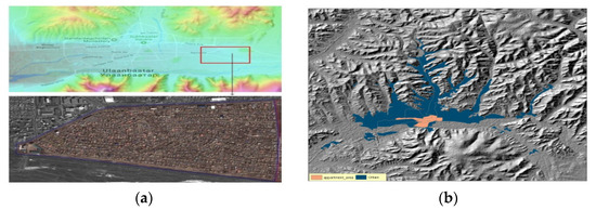
Figure 1.
Infrastructure of Ulaanbaatar (UB). (a) Geographical map of Ulaanbaatar (UB) and suburban areas. (b) Apartment area vs. ger district area.
Hence, the smoke from coal and other materials resulted in a horrifying situation in winter, as reported in some earlier works [5,6]. Before the government standardized fuel in Ulaanbaatar, in one example, the harmful dust level was 6–7 times higher than the most lenient World Health Organization standards, according to the World Bank Report in 2012 [7].
From 15 May 2018, the Government of Mongolia strictly banned the import and use of raw coal in Ulaanbaatar, and issued an order for the use of improved fuel instead. Hence, the air-quality index (AQI) has improved, and there was a big difference in the AQI between 2019 and 2020, especially in the wintertime. Consequently, the AQI is influential in addressing air-quality improvement because climatology contributed to improving fuels. However, the role of the AQI measurement network needs to be clarified. To be precise, even devices that accurately measure air quality are only informed by values of measurement from the past, with very few cases in real-time. Alternatively, the tools are simply about listening, i.e., how harmful the AQI was. In this situation, a predictive method may be the solution regarding the historical data information of the AQI, climatology, and improved fuel. Thus, we developed an embedded generative model for the AQI that depends on the environmental factor effect (EFE) influencing the AQI, which is a result of the city’s geographical features, such as temperature, wind, atmospheric pressure, etc., including improved and raw fuel measurement quantities.
Therefore, studying the interdependence between AQI and EFE with fuel measurement quantities is the purpose of this work. The variational autoencoder (VAE) and multilayer perceptron methods were used to develop an embedded generative approach. From the VAE learning, we produced new data based on its latent variables. Latent variables play a crucial role in VAE generation, highlighting data and reducing its dimensionality in a shallow space. The EFE with fuel measurement quantities was measured simultaneously with the AQI. The dimensions of the latent variables and the EFE with fuel measurement quantities were the same size. Hence, to discover the relationship between the AQI and the EFE data’s latent variable, a multilayer perceptron was used. Thirty-two variables were gathered in the EFE data, such as ambient temperature, pressure, and wind speed, as well as the impact of raw coal and improved fuel information. For the VAE learning process, a four-year period from 11 of Ulaanbaatar’s (UB’s) air-quality measurement networks were used. The proposed method’s results were evaluated by a Pearson chi-squared test and compared with a non-linear regression prediction in the final step.
The measurement quantities of raw coal and improved fuels in three different laboratories are shown in Table 1. The items in Table 1 are as follows: Q1—received basis refers to the moisture content of the coal (maximum percentage of water); Q2—dry basis ash content (maximum percentage of dry); Q3—dry basis volatile matter (maximum percentage of dry); Q4—total dry basis sulfur content (maximum percentage of dry); Q5—lower caloric value (kcal/kg min); Q6—percentage of carbon; Q7—percentage of hydrogen; Q8—percentage of nitrogen; and Q9—percentage of oxygen.

Table 1.
Fuel quality comparison.
Related Work on ANN and Deep Learning for Ambient Air Pollution Estimation
The application of a neural network (NN) for air pollution is associated with the development of an artificial neural network (ANN), with mainly machine learning and VAE being applied in prediction works. For instance, in early works, the ANN technique was applied for pollution prediction: Reich et al. used 24 h data for simple ANN architecture and discussed some of the limitations of the approach [8]. Moustris et al. used much larger meteorological and air pollution data to predict the pollution index of , , , and three days ahead in seven different places in Greece [9]. For urban air pollution prediction, an ANN was applied and compared with multiple time series methods, such as ARIMA, fuzzy time series, and principal component analysis (PCA), using 7–10 years of Malaysian air pollution measurement data [10,11,12]. A more expanded description of the ANN-based approach can be found in the review work in [13,14,15]. Furthermore, an ANN was used for the integrated assessment modeling of global climate change and ecological research [16,17].
Machine learning (ML) approaches have been applied for more automatic and accurate air pollution predictions from a large amount of input data with numerous outputs. Zhang et al. studied the superior predictive ability of ML methods based on six years of Hong Kong air-quality index measurements [18]. Moreover, the special gradient-boosting ML approach was applied for predicting the concentration in China [19]. Delavar et al. used an autoregressive non-linear neural network with an external input for improving air pollution prediction in the case of Tehran city [20]. The research of Ly et al. considered the dependence between the pollution index and the sources obtained from multisensory measurements and weather data in air pollution predictive analysis-based ML approaches [21]. Similar work was reported by Arnaudo et al. in the urban area of Milan city using different configurations employing machine and deep learning models, such as a linear regressor, an artificial neural network using Bayesian regularization, a random forest regressor, and a long short-term memory network [22].
Lee et al. presented a gradient boosting–based machine learning approach for predicting concentration based on a large-scale data set in Taiwan city [23]. For UB city, concentration prediction has been studied using two different ML approaches, and high-performance results have shown the spatiotemporal variations in the high-emission areas [24]. Moreover, Meredith et al. compared several machine learning methods for ground-level pollutant mixtures of particulate matter with a diameter smaller than for air-quality assessment in Mongolia [25]. The survey works of ML methods for ambient air pollution assessment are summarized in [26,27,28,29,30].
Among the generative models for air contamination, deep learning methods are a more recently developed approach. Tien et al. worked on air-quality inference based on a graph-based matrix completion problem, and applied a variational model on graph convolutional autoencoders [31]. Additionally, they used a mobile Internet of Things sensor for fine-grained air quality in deep learning inference [32]. The spatiotemporal prediction of air pollution based on deep learning approaches has been studied widely for many different purposes. Li et al. studied the spatiotemporal deep learning–based air-quality prediction method that inherently considers the spatial and temporal correlations and prediction results of all stations compared with traditional time series prediction models [33].
Li et al. introduced the advantage of using two-stage models in geographically weighted machine learning [34], and deep learning to robustly impute a long time series of multi-angle implementation of atmospheric correction aerosol optical depth [35]. The achievements of embedded methods with deep learning approaches were considered in [36,37], and the high performance of autoencoder-based residual networks consisting of learning models is analyzed in [38].
Fan et al. studied the framework and feasibility of an idea based on deep RNN [39], whereas improved feature analysis was considered in [40] based on fine-grained air quality.
2. Methodology
2.1. Area of Study and Data Collection
The capital city UB has a history spanning more than 360 years and is currently home to 50% of the country’s population. This population is continuously growing; therefore, the most significant problem is in an urban ecological context, with environmental pollution also dramatically increasing. In addition, the city has a harsh and unique climate, and its geographical location behavior is the main cause of this air pollution. The city is located in a large valley surrounded by mountains, at an elevation of approximately 1580 m above sea level. Due to the elevation and being located far from the sea, the city has a very long-lasting winter, making UB one of the coldest capital cities in the world. Ulaanbaatar receives an average of 239 mm of precipitation per year, of which 1 mm or more falls in 39 days, and 5 mm or more of rain falls in 15 days. Generally, this area is arid, with the humidity sometimes decreasing to 4% per year. The wind comes mainly along the valley, but the strength of the wind is low throughout the year, with 10% of the wind observed in the spring months.
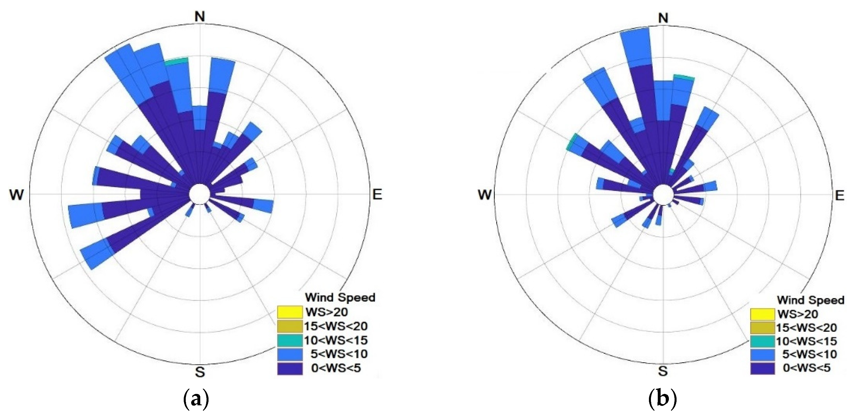
The average annual surface air temperature is −0.7 °C, dropping to −45 °C in the winter and warming up to +59 °C in the summer. Sudden frosts occur on the surface of the soil in all months except July. Therefore, the ground freezes to a considerable depth of 4–8 m. The average wind speed for the country is less than 2 m/s, which affects the air pollution levels, making them more constant for an extended time. Additionally, the average wind speed of the capital city is primarily 0.5 m/s from the northern and northwestern areas, which means that there is not much air circulation. Thus, air pollution remains stable for long periods around the center of the city. Figure 2 shows the wind information maps across four years.

Figure 2.
The wind direction and speed map of UB city. (a) The 2016 wind rose map. (b) The 2019 wind rose map.
The National Agency for Meteorology and Environmental Monitoring (NAMEM) established the first air-quality monitoring station in Ulaanbaatar in 1977. This was the foundation for the establishment of an air-quality monitoring network in Mongolia. Until 2008, there were four permanent air-quality monitoring stations in Ulaanbaatar, which measured only two indicators, sulfur dioxide and nitrogen dioxide. There was no continuous air-monitoring system built on the outskirts of Ulaanbaatar city.
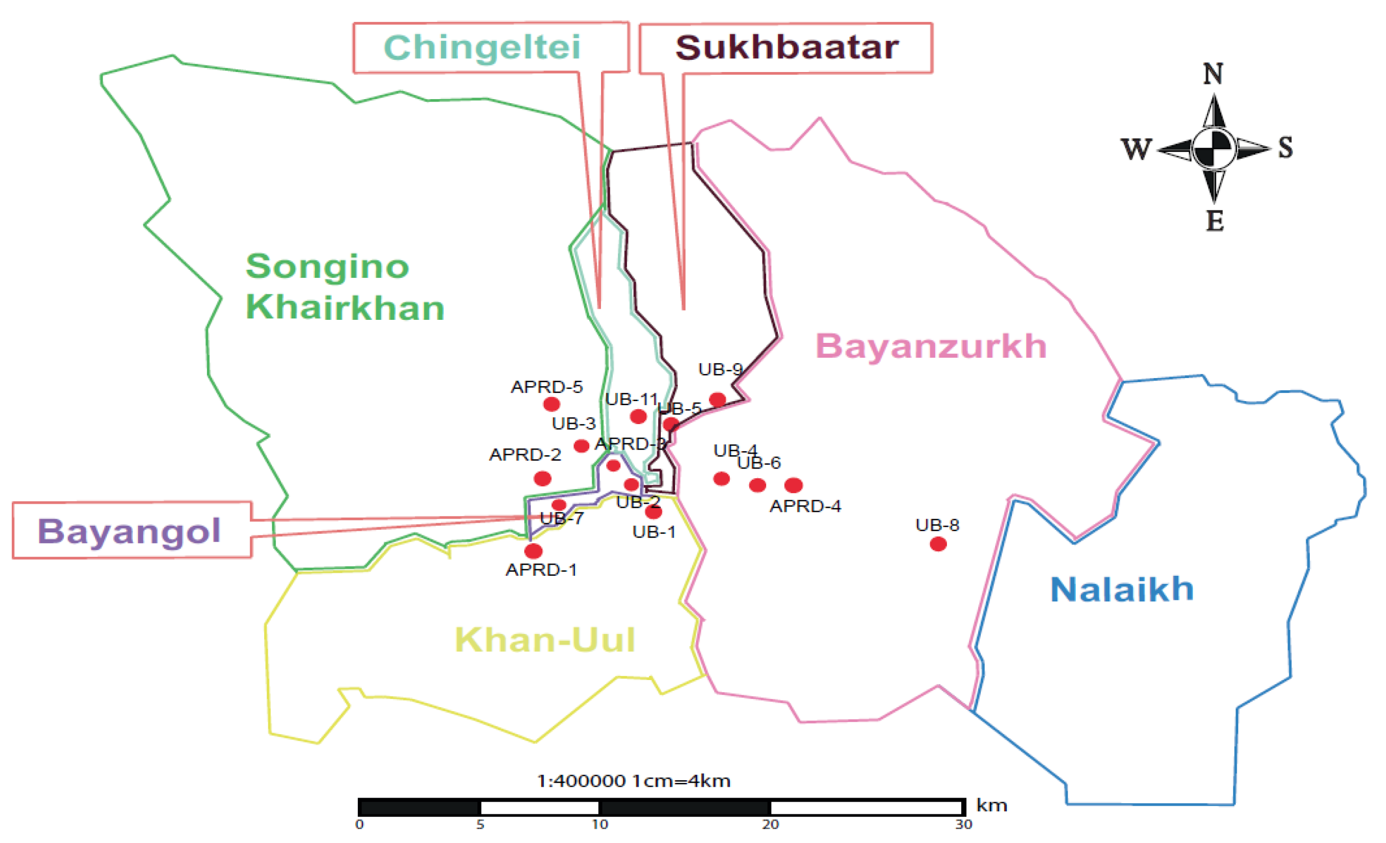
Due to Ulaanbaatar’s air pollution issues, there is a need to expand the network by equipping it with automatic, continuous measurement capabilities and improving its capacity. The air-quality monitoring network consists of the Air Pollution Reducing Department of Capital City (APRD) Network and the NAMEM Network. A German grant established the APRD Network with five stations in 2008, and the NAMEM Network, with 10 stations, was established by means of a French loan in 2010. Currently, 12 automatic stations are measuring sulfur dioxide, nitrogen oxides, carbon monoxide, ozone, , and every 15–30 min, and 3 non-automatic controls of sulfur dioxide and nitrogen dioxide (Figure 3). The concentration is determined using a chemical solution.
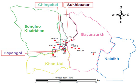
Figure 3.
State map of UB and air-quality index (AQI) measurement networks.
2.2. VAE for Embedded Generative Method
Let be the AQI measurements collected from measurement networks at different locations in the city. Furthermore, represents the EFE of the air quality, which is measured at the same time as . Next, the purpose is to understand the relationship between those two quantities; . In the case of air quality, the relationship is completely unknown; generally, it is assumed to be a system of highly non-linear maps. Moreover, data of and raw and sampling methods are very different in each measurement. In this situation, a variational autoencoder (VAE) has the benefit of representing the data in low dimensional continuous latent variables with intractable posterior distributions [41].
The VAE method optimizes the weight parameters and bias of the function: , which is a non-linear approximation of the relation map, as follows:
where is the data set provided and stored from the relation map . The optimization process of consists of two maps, encoder Φ and decoder Ψ. The encoder reduces the dimension of y into dimensionally reduced space, Φ: → , and then the decoder map generates new values from the reduced space, Ψ: → . Thus, when an optimal parameter is reached, we obtain the pair of which satisfies the following minimization:
where is the Kullback–Leibler (KL) divergence loss between and (along with this formulation, we refer [42,43]). KL measures how the distribution of associated with data is different to the normal distribution, defined as:
where l is the dimension of dimensionally reduced space , called latent space. To obtain the latent space from the data, the multilayer perceptron (MLP) is the advised method. The map of reducing dimension consists of several hidden layers, and every layer has finite nodes. In the encoder process, the number of nodes in the steps of layer is conventional in reducing the order. is denoted as the weight parameters of the layers between kth and (k + 1)th, whereas i and j are node positions, respectively. Then, the kth layer weight parameters can be represented in the following matrix form:
where m is the number of notes in the kth layer, and n is the number of nodes in the (k + 1)th layer. To curtail the dimension of input that the number of nodes in the layer satisfies:
In recurrent form, this can be described as:
where refers to the bias parameters and is the matrix transpose operation. Every retains the key feature of the previous steps, and the final space is considered to be the feature space. Then, the encoder function is represented as:
where is the sigmoid function. The main feature that distinguishes a VAE from other generating models is its latent space. If we look at latent space alone, its actual value is a quantity that cannot be measured directly. However, it contains the core of the essential information in the data, determining in the latent space the KL-divergence loss and reparameterization trick is vital. In the process of optimization, Equation (3) provides a close distribution to normal with and expressed as:
where , , , and are the weight and bias for and . Then, the latent variable is described as:
where is the normally distributed auxiliary noise variable and is the element-wise product. Figure 4 shows the reparameterization trick on , the difference with and without is intractable posterior distributions.
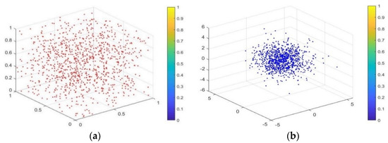
Figure 4.
The reparameterization trick on (a) The random sample of and . (b) The random sample of and with .
More precisely, the latent space is centered at the coordinate and distributed in a bounded interval in any direction; thus, any linear combination between two points of the space belongs to its space (for more detailed properties of this phenomena, refer to Section 3.4 of [42]).
When variables are found, the decoder function is defined as:
Then, the entire process of VAE is to determine the parameters of and , where:
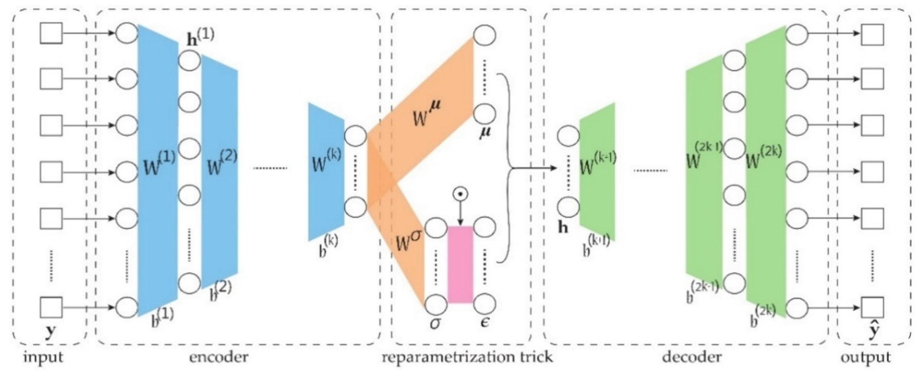
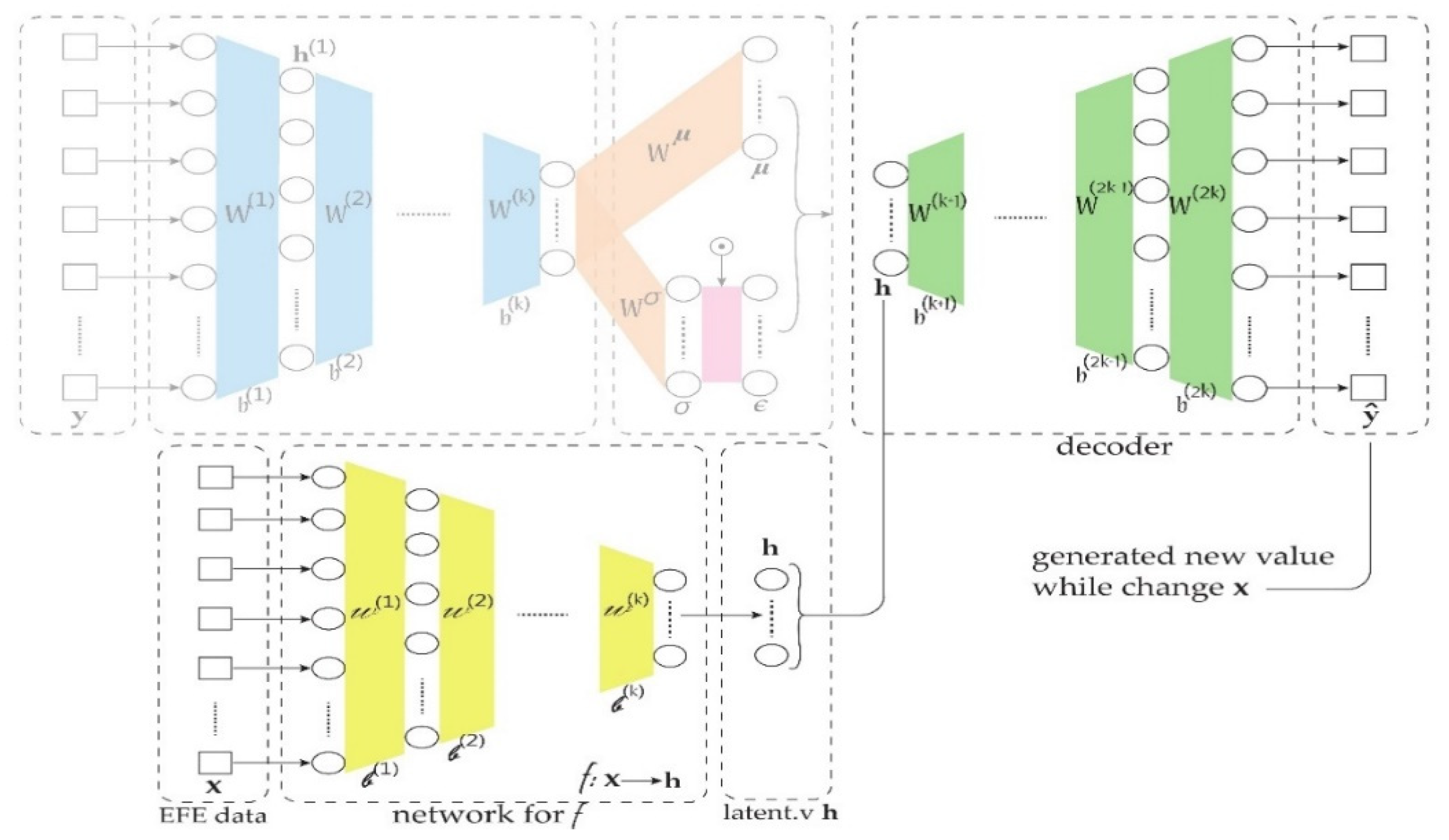
The process of optimizing those parameters is based on backpropagation and a gradient descent algorithm. Initially, it starts with random choice in and , then the sensitiveness of training errors in little changes in those parameters, and the derivative of the training error leads to the chain rule and backpropagation. The network architecture is represented in Figure 5, and the architecture of the VAE, and the algorithm of optimizing the parameters, are described in the next section, along with the embedded network.
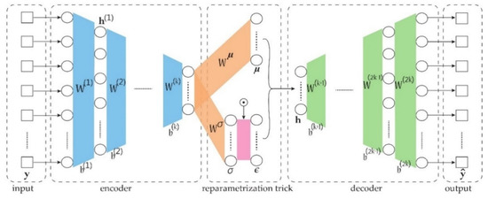
Figure 5.
The architecture of the variational autoencoder (VAE).
2.3. Embedding Network for the Relationship between EFE and AQI
The formulas described in Equations (2)–(13) are basic VAE methods for generating new AQI values from the latent variables obtained in the learning process. In order to approximate the function F, whereby , and are as described in Equation (1), we need different approaches to the typical VAE approach. However, the method defined in Equations (2)–(13) determines the vital space of the AQI, which is the latent variable . To find the relationship between latent space data and the EFE, we use the feedforward neural network approach, as the period of sampling time is equal.
Expressly, the first column of Equation (14) represents n daily measurements of AQI, and the next column is the latent variables obtained through the algorithm applied to daily measurements of the AQI. Additionally, EFEs were also measured on the same day with :
Hence, the data are available to learn the relationship between and . Apply the feedforward neural network to approximate the function ; indeed, it is the universal approximation theorem for . Thus, it gives the function, which is an approximation function as with weight and bias parameters corresponding to network nodes. Then, the new generating AQI values can be described through the embedding as:
The architecture of the two combined networks is represented between , , and in Figure 6.
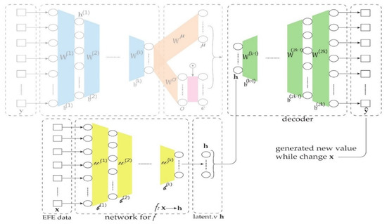
Figure 6.
The architecture of the embedded network.
The Algorithm 1 for the embedded generative model:
| Algorithm 1: embedded modeling algorithm |
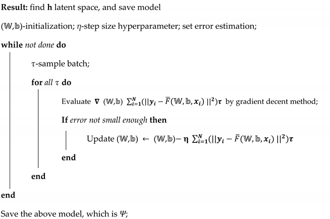 |
| Result: find the relation map ƒ; (,)-initialization; ζ-step size hyperparameter; set error estimation; set algorithm for (,) same with (,); |
| Result: embedding of Ψ, ƒ; Generate new AQI values based on the embedding; Ψ: (ƒ: x h) ŷ |
3. Experiment
3.1. Data Expression
To validate the proposed method of illustrating the interdependency between AQI and EFE, we used four years of air pollution concentration measurements and four years of weather data. The correlation between AQI and pollution concentration is defined as:
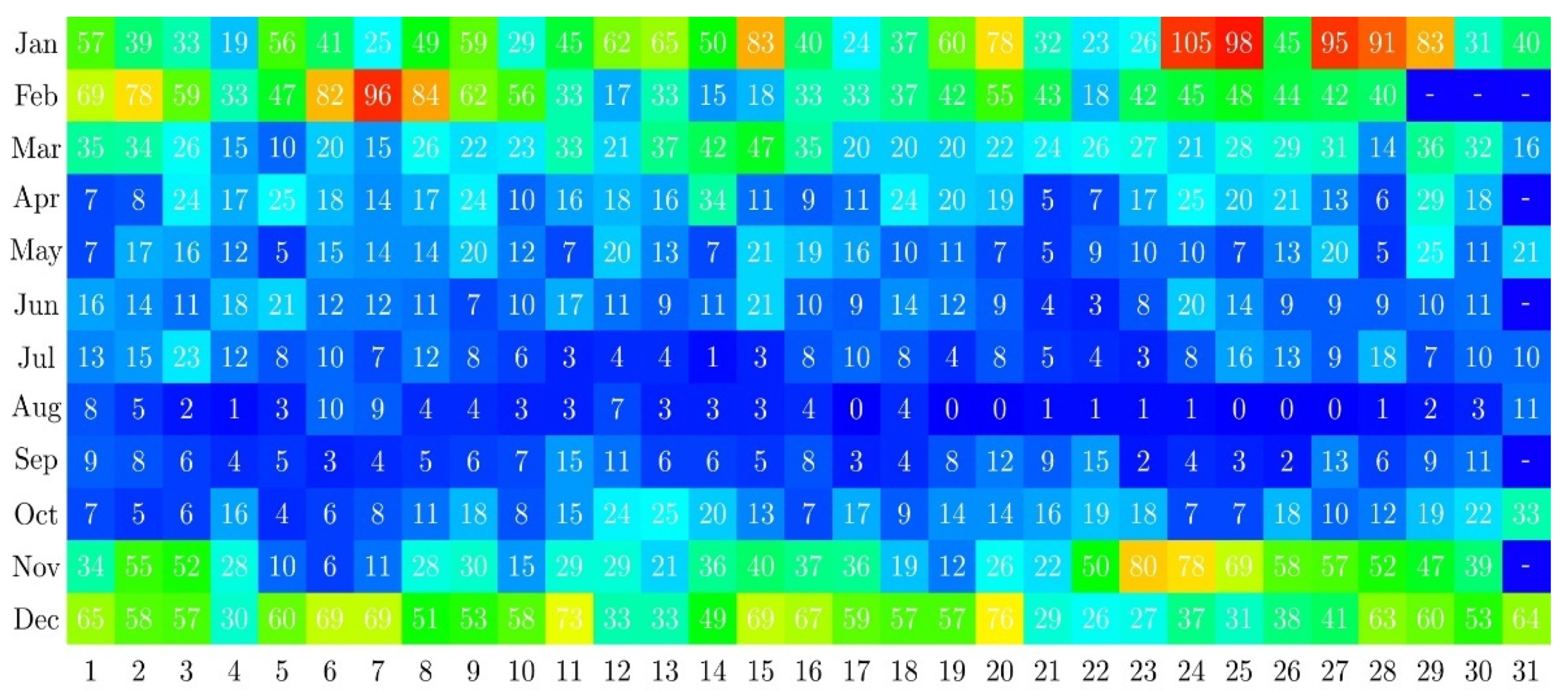
where is the amount of pollutant concentration per cubic meter of air, and are the lowest and highest breakpoints of , and and are the index breakpoints corresponding to and . However, the AQI is designed to disseminate air-quality information using color coding as it is accessible to the general public, normalizing the measurement into world standards, with the relationship between AQI and being direct one-to-one. Furthermore, the pollutant concentration is available from measurement stations, with most of them even working automatically, and we used instead of AQI. In addition, the pollution concentration data that were assembled between 1 January 2016 and 1 June 2020 from 15 pollution measurement stations and positions are shown in Figure 3. Three of them determined the pollution concentration based on active sampling tests, and the remaining stations automatically measured the concentration. The automatic stations used the light source to obtain the signal difference between the reference and the incoming air in sampling manifolds. This working principle analyzed the amount of different pollution concentrations by micrograms per cubic meter in a minute and eliminated rotation for optic adjustment. Related to the working principle and purpose, each station had different measuring capabilities, namely measured from 15 stations, measured from 13 stations, measured from 14 stations, measured from 8 stations, and measured from 10 stations, with a total of 60 pollution concentrations gathered for the experiment. As in the example, the daily concentration of in 2016 is expressed in Figure 7, which was measured by UB-2, with the tolerable content level being .
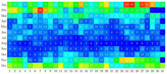
Figure 7.
The daily concentration of in 2016, measured by UB-2, tolerable content level is .
The EFE data were composed of measurements of a comprehensive range of weather data sampled from five automatic weather measurement stations in UB. Weather data involve various levels of wind speed, wind direction, temperature, relative humidity, and the most crucial information for the fuel period. Furthermore, weather information was collected within the same period as the air pollution concentration measurement.
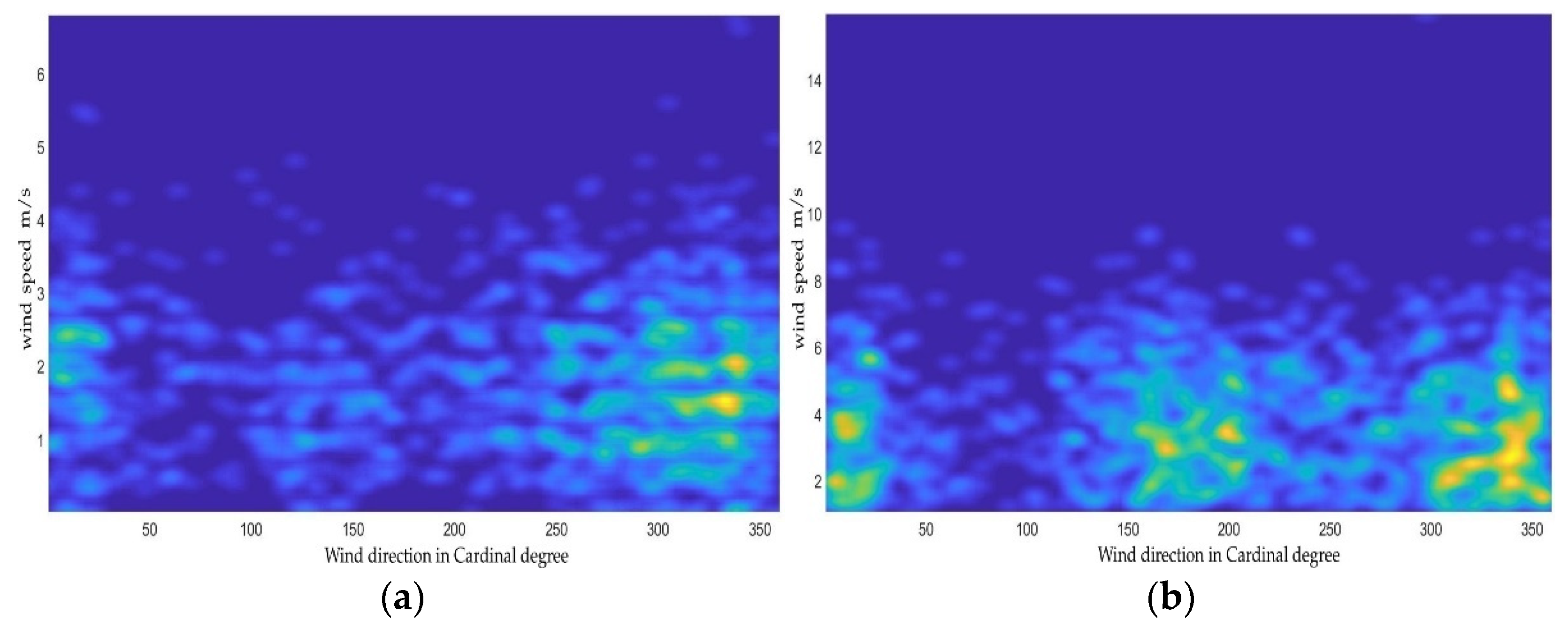
Surface wind regimes depend on local climatic conditions and atmospheric circulation. Each season, the average wind speeds are very different in UB, in spring, in winter, and in other seasons. In winter, due to the strong anti-cyclones, the prevailing wind speed slows down, whereas in other seasons, the west, northwest, and north winds prevail along the prevailing air flow. Depending on the location of the weather stations in UB, the wind direction, speed, and frequency are quite varied. For example, in the station at the airport, the east wind is predominant in all seasons except spring, different to the station at the university. The four years of the probability distribution of the direction and wind speed are visualized in Figure 8. The degree of wind direction is defined in cardinal degrees as compass points.

Figure 8.
The distribution of wind with respect to direction and speed in 2016–2019. (a) The station at the university. (b) The station at the airport.
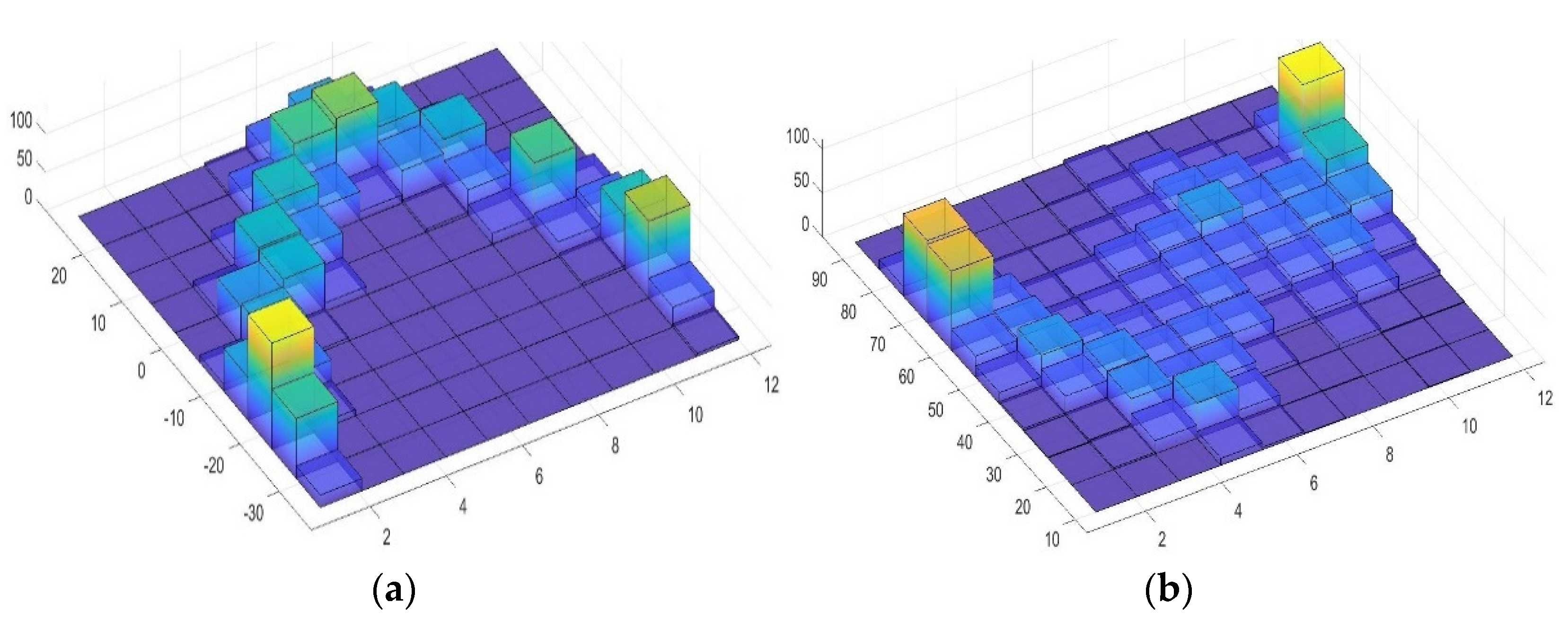
Furthermore, four years of temperature and relative humidity information are expressed in Figure 9. For both quantities, the frequency is counted with respect to amounts of years, and the absolute measurements are represented in a bivariate histogram. In the illustration of temperature, the higher frequencies appear more often in the cold season over the four years of data than in the warm season. The amount of relative humidity is inversely related to air temperature and depends on cloud precipitation. The average annual relative humidity around Ulaanbaatar is 55–76%.

Figure 9.
The bivariate histogram expression of temperature and humidity in 2016–2019. (a) Temperature. (b) Humidity.
3.2. Visualization of the Results
In the VAE-based learning process, to obtain the feature space of the AQI data, we need to separate data into two parts, i.e., training and testing. The data size was 365 60 = 87,600 from 8–15 air pollution concentration measuring stations, and the data were separated into 60,000 and 27,600 for training and testing, respectively. The computation architecture for the VAE consisted of three hidden layers with nodes 40, 30, and 20, and one input channel had a length of 60. The training epoch was 200,000, the batch size was 1000, and the learning rate was 0.001. We used an RmsProp optimizer with the ReLU activation function in the hidden layer and the sigmoid activation function in the output layer.
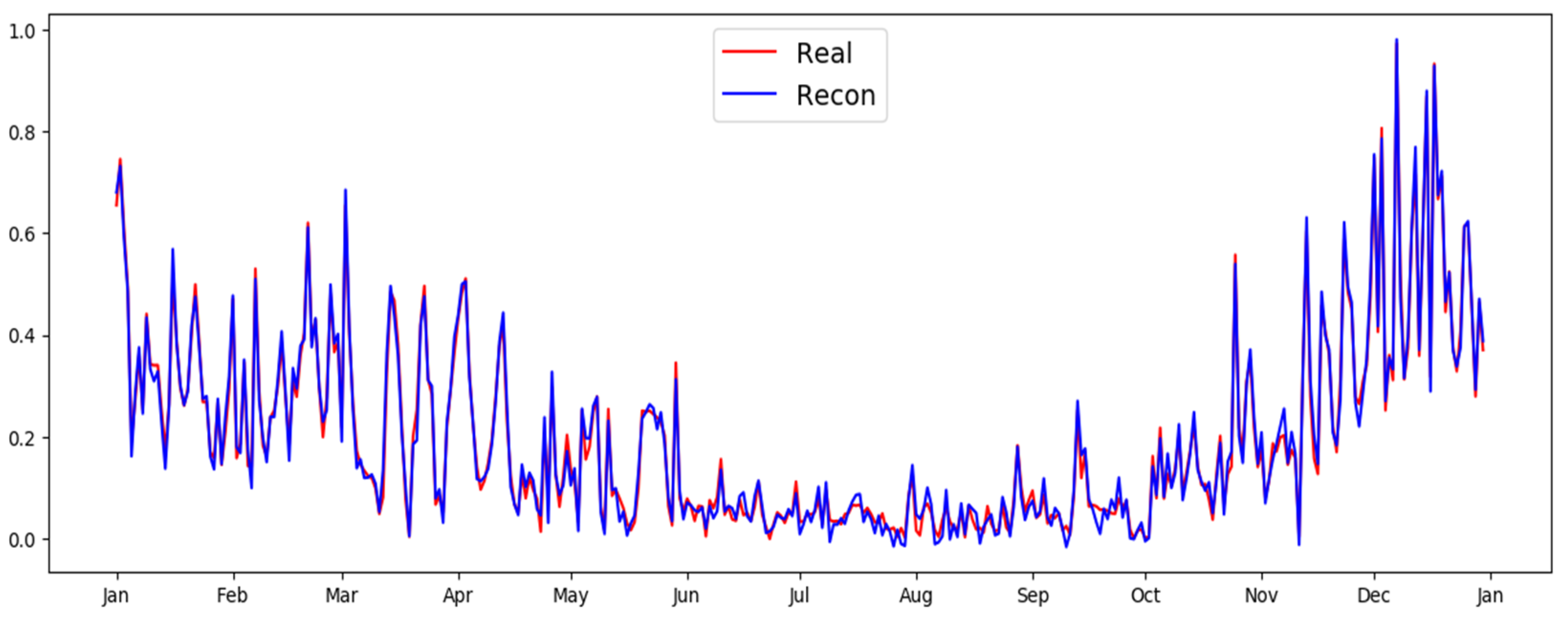
Python and TensorFlow were used for the VAE implementation, and a PC equipped with an Intel(R) Core (TM) i7-2600-CPU@3.40GHz, with an NVIDIA GeForce GTX 1060ti 6GB GPU was used for the computation. The Python plotting tool, MATLAB, and LaTeX pgfplot packages were used in the data and result visualization. In Figure A1, Figure A2 and Figure A3 in the Appendix A, the typical air pollution measurement of and the convergence rate of the VAE computation at a particular epoch are shown.
With this latent space computation, we completed the VAE using the algorithm illustrated in pseudocode 1. Next, for the relationship between the EFE data and the latent variables of the VAE, the development of a feedforward NN for learning was required, which is observed in the second step of pseudocode 1. The daily measurement of the EFEs consisted of 32 quantities. Hence, the feedforward NN’s input channel was 32, and it had one hidden layer with 25 nodes. Along with a training epoch of 10,000, a batch size of 20, and a learning rate of 0.001, we used the Adam optimizer with the ReLU activation function in the hidden layer and the sigmoid activation function in the output layer, whereas 70% and 30% of the data were used for the training and testing sets, respectively.
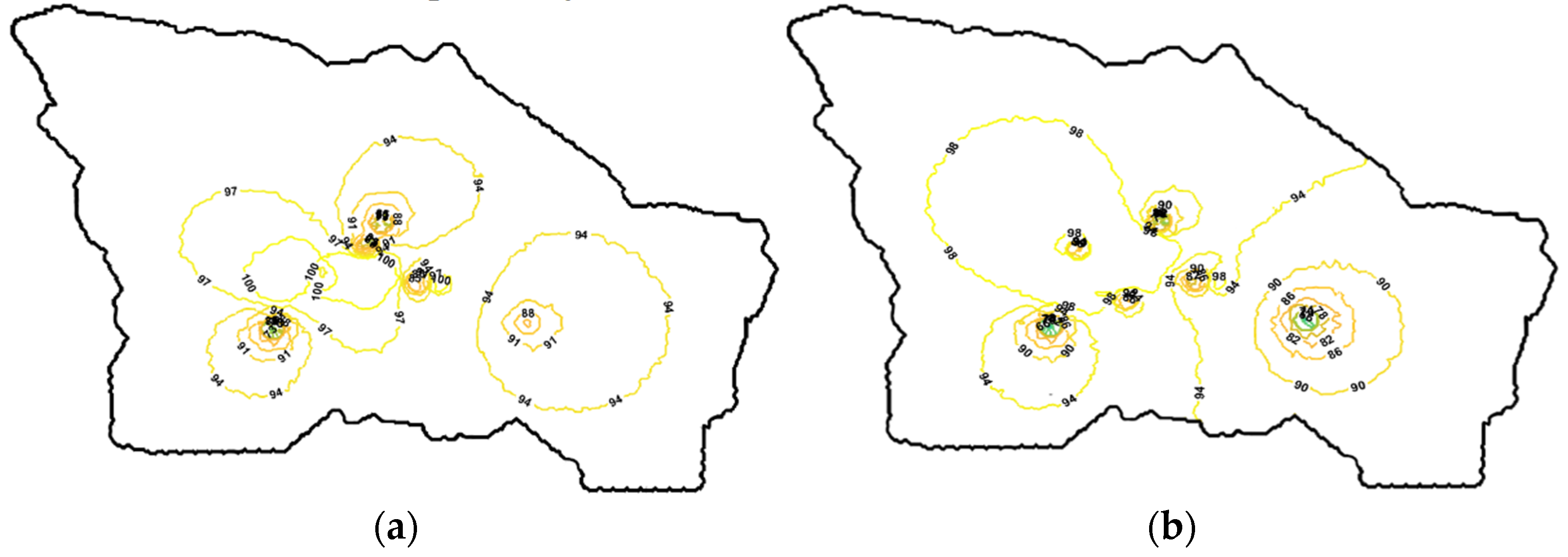
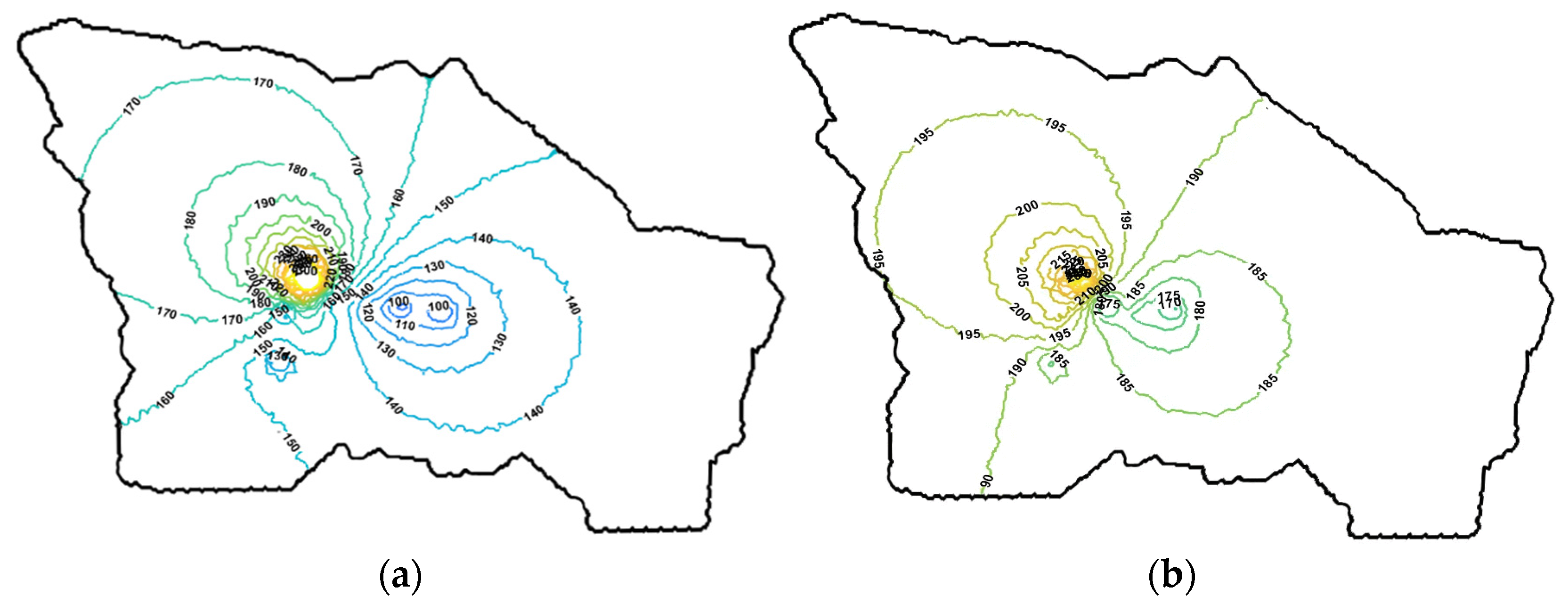
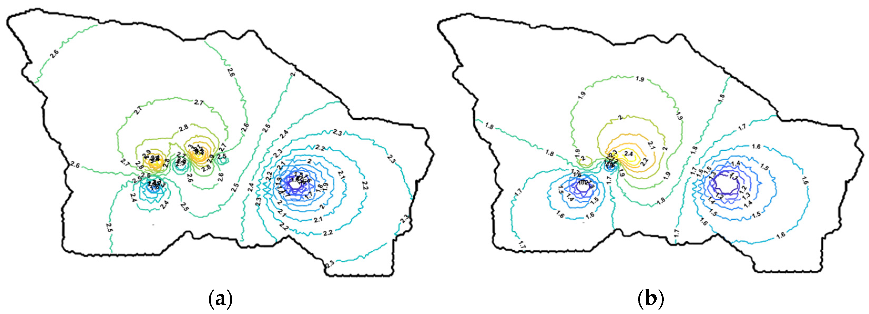
Finally, to validate our suggested method, the EFE data of the first three months of 2020 were selected for generating the predicted air pollution concentration. With respect to the first 90 days and the pollution measurement stations, the model provides 90 60 = 5400 as the number of results. This large number of results requires an expression of the outcome in an optimal way, and we elected a few specific depictions. For this reason, the most frequently polluted days of each pollution index were chosen to illustrate the results. Table 2 represents the most frequently polluted dates in the first three months of our four years of data.

Table 2.
The most frequently polluted air pollution dates in 2016–2019.
The coldest days of the year directly affected the reason for representing the same behavior for gaseous pollution in the first three months of integration in Table 2. By long-standing average, the coldest days of the year are between 8 and 15 January. Therefore, in January, , , and are formed from fuels burned in home stoves for heating in the ger districts with high atmospheric pressure and temperature inversion. However, particular pollution is related to poor infrastructure. When the warm season starts, particular pollution from the ger districts increases due to the mobility of a large number of vehicles; consequently, at the end of March, the measurement of greatly increases.
Furthermore, the inverse distance weight (IDW) interpolation method was used for the pollution concentration map. The inverse weight is defined as:
where is the number of points for interpolation, and is distance between the th interpolation point and the jth air pollution measurement station. Then, based on Equations (14) and (15), the concentration values at the th interpolation point is estimated as:
The results of Equation (18) are expressed in Figure 10, Figure 11 and Figure 12, corresponding to the integrated values in Table 2; 1 February and March for and , and 11 January for were selected, respectively.
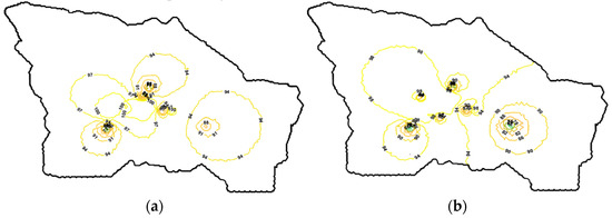
Figure 10.
The distribution map of on 1 February 2020. (a) The distribution of actual . (b) The distribution of predicted .
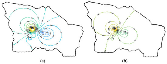
Figure 11.
The distribution map of on 11 January 2020. (a) The distribution of actual . (b) The distribution of predicted .

Figure 12.
The distribution map of on 1 March 2020. (a) The distribution of actual . (b) The distribution of predicted .
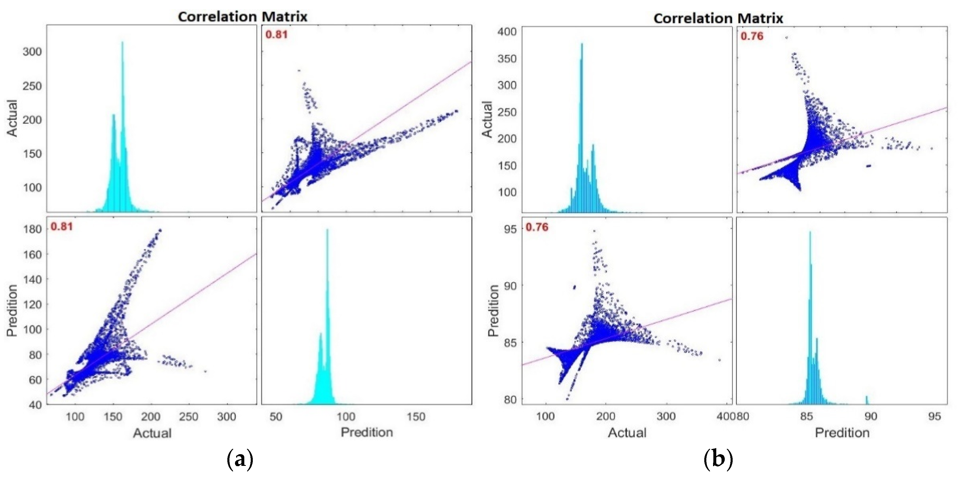
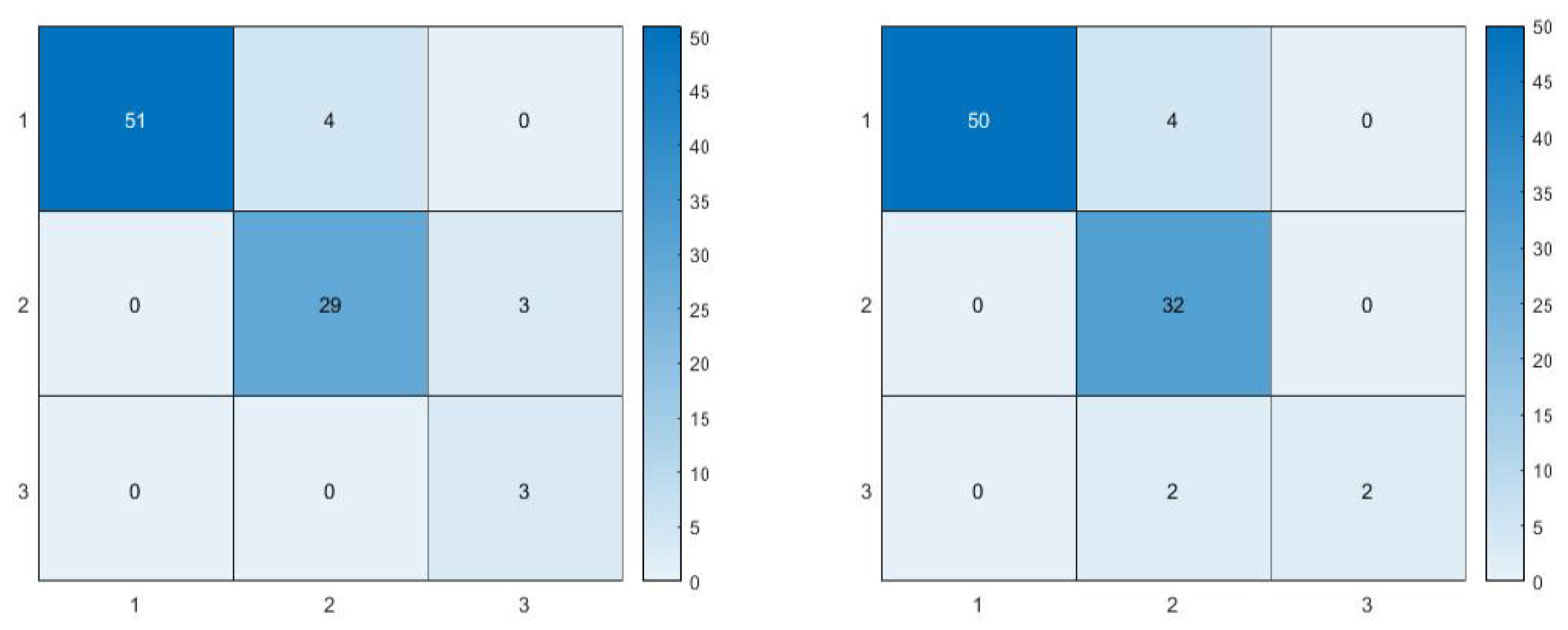
For more results, we randomly selected one of the pollution measuring stations for every five air pollutions, and 90 days of both actual and model prediction results are compared in Appendix A. To evaluate the performance of the proposed model, the most commonly used correlation coefficient and Pearson’s chi-squared methods were used. The positive correlation coefficient indicates higher correlation between testing values. As in the example, Figure 13 and Figure 14 represent the correlation coefficients between the actual and predicted values of , , , and obtained from all measurement stations, respectively. In the figure, the corresponding correlation coefficients are highlighted in red in the correlation matrix plot. For more validation purpose, we randomly selected one measurement station and computed the contingency tables for 90 days of actual and predicted values, which expressed in Figure A4, Figure A5, Figure A6, Figure A7 and Figure A8 in Appendix A. Two of the corresponding contingency tables for and are shown in Figure A9.
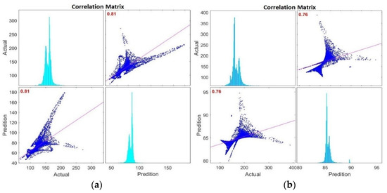
Figure 13.
The correlation matrix of actual and predicted values. (a) (b) .
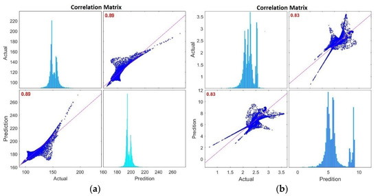
Figure 14.
The correlation matrix of actual and predicted values. (a) , (b) .
For the remaining three air pollution concentrations, the contingency table was similar, whereas the average chi-squared result was . Thus, the statistics for the Pearson’s chi-squared test were highly dependent on each other.
4. Conclusions
In this study, a variational autoencoder-based embedded generative air pollution model was developed. The proposed approach represented substantial progress in the reliable prediction of five air pollution concentrations. The embedded generative model consists of a VAE and a feedforward NN to discover the relationship between the air pollution concentration and environmental factor effects. The convergence of learning networks based on the gradient descent method with RmsProp and Adam optimizer techniques were applied, and the convergence rate was , consequentially. To construct the proposed model, we simultaneously assembled four years (2016–2020) of air pollution concentration measurements and weather data. In addition, information on improved and raw fuel was involved in the environment factor data. The prediction values of the model corresponded to all the pollution measurement stations, with a total of 15 90 = 1350 prediction values obtained for the test with respect to 15 stations in the first 90 days of 2020. Thus, the results can be visualized in two ways. First, a pollution map can be created by using the inverse distance weight interpolation throughout the regions of UB, which expresses a daily pollution map for estimating the pollution concentration for local coordinates of the city. For instance, the difference between the local measurement and the prediction results for in ger district areas located in UB suburbs in four directions was 21.24 , −9.32 , 11.05 , and −11.87 , respectively, in the Airport, Zuragt, Tolgoit, and Amgalan districts on 16 January 2020. The correlation coefficient method was applied while constructing the pollution concentration map of the city for each pollution index, and the average of these indicates the entire performance of the model as 0.8280. The Pearson’s chi-squared test method was used for testing the second visualization performance of the individual pollution measuring stations and expressed a high correlation between actual and predicted. A further aim of considering the VAE and NN embedding to investigate inversely the interdependencies between the weather and the fuel conditions, by sampling normal to good days of air pollution, could be considered for future study.
Author Contributions
Conceptualization, B.B. and M.T.; methodology, B.B., M.T. and L.S.; investigation, B.B., M.T. and L.S.; writing—original draft preparation, B.B., M.T., L.S. and A.B.; writing—review and editing, M.T. All authors have read and agreed to the published version of the manuscript.
Funding
This research received no external funding.
Institutional Review Board Statement
Not applicable.
Informed Consent Statement
Not applicable.
Data Availability Statement
The datasets used and/or analysed during the current study are available from the corresponding author on reasonable request.
Conflicts of Interest
The authors declare no conflict of interest.
Appendix A
The convergence rate of the VAE computation at a particular epoch. We designed two methods to compare the results of the embedded model with real measurements. The first way was represented in Figure 10, Figure 11 and Figure 12, in which we gathered results belonging to all measurement stations and used the IDW method to construct a concentration map for one day. For the second way, we chose one station and sampled the results concerning the days that EFE was applied to the model. In this way, we applied the first 90 days’ data of 2020 for EFE to the (15), the model provided 59 90 values.
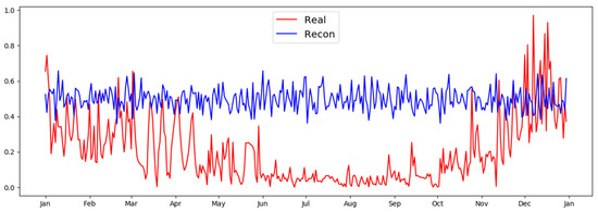
Figure A1.
Convergence of the VAE computation at the first epoch.
Figure A1.
Convergence of the VAE computation at the first epoch.
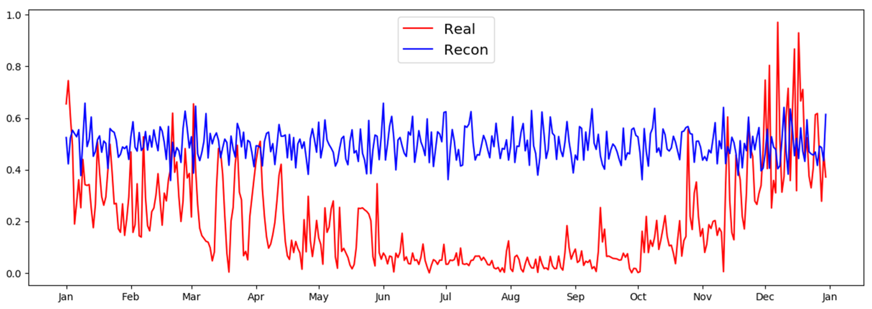

Figure A2.
Convergence of the VAE computation at an epoch of 400.
Figure A2.
Convergence of the VAE computation at an epoch of 400.
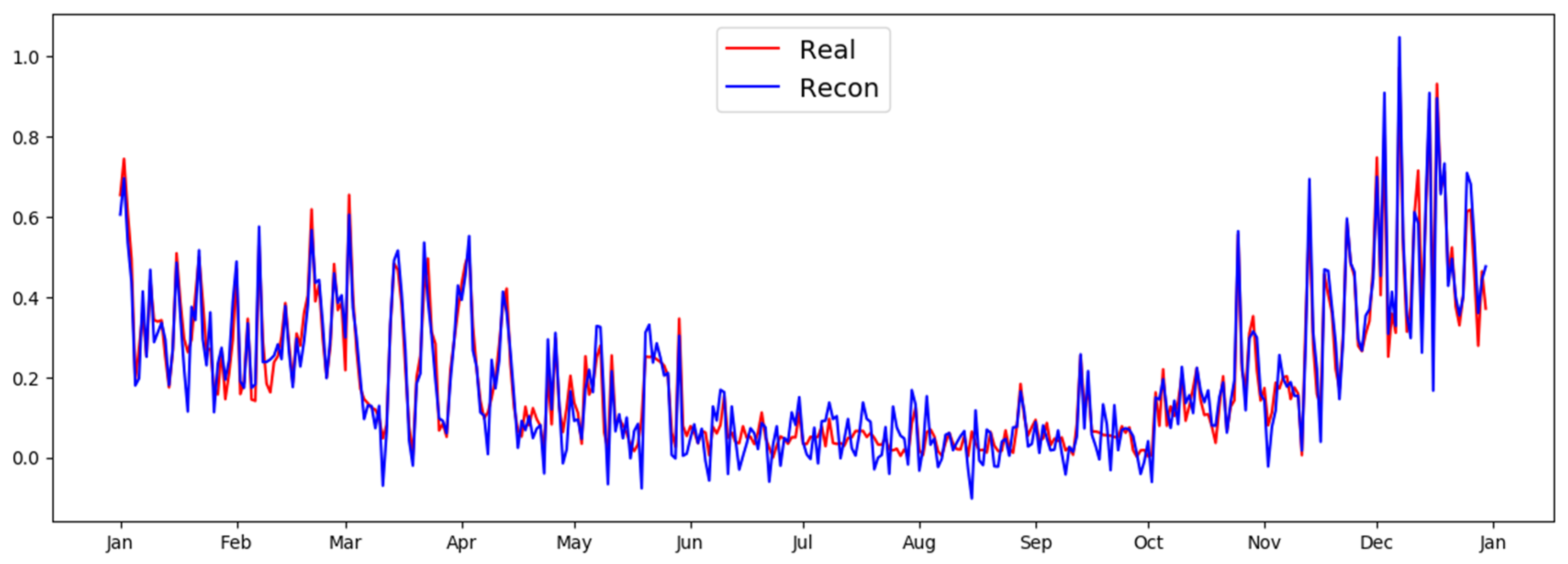

Figure A3.
Convergence of the VAE computation at an epoch of 800.
Figure A3.
Convergence of the VAE computation at an epoch of 800.
From the results of 59 stations, we randomly chose the station and compared the 90 days of results to the actual measurements (Figure A4, Figure A5 and Figure A6). In Figure A4, the real and predictive values of for the UB-5 station are presented. Meanwhile, Figure A5 shows the graphics of the actual measurement and the predictive results of the embedded model of for the UB-7 station. Additionally, in Figure A6, the graphics of the real measurement and the predictive values of the method for for the APRD-2 station are expressed.

Figure A4.
The first three months of 2020, the absolute measurement, and the predictive results of the model for , at the UB-5 station.
Figure A4.
The first three months of 2020, the absolute measurement, and the predictive results of the model for , at the UB-5 station.


Figure A5.
The first three months of 2020, the absolute measurement, and the predictive results of the model for SO2, at the UB-7 station.
Figure A5.
The first three months of 2020, the absolute measurement, and the predictive results of the model for SO2, at the UB-7 station.


Figure A6.
The first three months of 2020, the absolute measurement, and the predictive results of the model for , at the APRD-2 station.
Figure A6.
The first three months of 2020, the absolute measurement, and the predictive results of the model for , at the APRD-2 station.

The two graphics in Figure A7 and Figure A8 show a comparison of the real and predicted values of the method for the UB-1 station, as well as the prediction of for the APRD-4 station, respectively.

Figure A7.
The first three months of 2020, the absolute measurement, and the predictive results of the model for , at the UB-1 station.
Figure A7.
The first three months of 2020, the absolute measurement, and the predictive results of the model for , at the UB-1 station.


Figure A8.
The first three months of 2020, the absolute measurement, and the predictive results of the model for , at the APRD-4 station.
Figure A8.
The first three months of 2020, the absolute measurement, and the predictive results of the model for , at the APRD-4 station.

Two of the corresponding contingency tables for and are shown in the following figure.
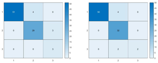
Figure A9.
Contingency tables for and .
Figure A9.
Contingency tables for and .
References
- Ritchie, H. Urbanization. 2018. Available online: https://ourworldindata.org/urbanization (accessed on 25 December 2021).
- Ganbat, G.; Baik, J.J. Wintertime winds in and around the Ulaanbaatar metropolitan area in the presence of a temperature inversion. Asia-Pac. J. Atmos. Sci. 2016, 52, 309–325. [Google Scholar] [CrossRef]
- Byamba, B.; Ishikawa, M. Municipal Solid Waste Management in Ulaanbaatar, Mongolia: Systems Analysis. Sustainability 2017, 9, 896. [Google Scholar] [CrossRef]
- World Bank. Air Quality Analysis of Ulaanbaatar: Improving Air Quality to Reduce Health Impacts. 2011. Available online: https://openknowledge.worldbank.org/handle/10986/26802 (accessed on 25 December 2021).
- Guttikunda, S.K.; Lodoysamba, S.; Bulgansaikhan, B.; Dashdondog, B. Particulate pollution in Ulaanbaatar, Mongolia. Air Qual. Atmos. Health 2013, 6, 589–601. [Google Scholar] [CrossRef]
- Luvsan, M.-E.; Shie, R.-H.; Purevdorj, T.; Badarch, L.; Baldorj, B.; Chan, C.-C. The influence of emission sources and meteorological conditions on SO2 pollution in Mongolia. Atmos. Environ. 2012, 61, 542–549. [Google Scholar] [CrossRef]
- Curbing Air Pollution in Mongolia’s Capital, World Bank Report. 2012. Available online: https://www.worldbank.org/en/news/feature/2012/04/25/curbing-air-pollution-in-mongolia-capital (accessed on 25 December 2021).
- Reich, S.; Gomez, D.; Dawidowski, L. Artificial neural network for the identification of unknown air pollution sources. Atmos. Environ. 1999, 33, 3045–3052. [Google Scholar] [CrossRef]
- Moustris, K.P.; Ziomas, I.C.; Paliatsos, A.G. 3-Day-Ahead Forecasting of Regional Pollution Index for the Pollutants NO2, CO, SO2, and O3 Using Artificial Neural Networks in Athens, Greece. Water Air Soil Pollut. 2010, 209, 29–43. [Google Scholar] [CrossRef]
- Rahman, N.L.; Muhammad, H.; Latif, M.T.; Suhartono, S. Forecasting of Air Pollution Index with Artificial Neural Network. J. Teknol. 2013, 63, 59–64. [Google Scholar] [CrossRef]
- Azid, A.; Juahir, H.; Toriman, M.E.; Kamarudin, M.K.A.; Saudi, A.S.M.; Hasnam, C.N.C.; Aziz, N.A.A.; Azaman, F.; Latif, M.T.; Zainuddin, S.F.M.; et al. Prediction of the Level of Air Pollution Using Principal Component Analysis and Artificial Neural Network Techniques: A Case Study in Malaysia. Water Air Soil Pollut. 2014, 225, 2063. [Google Scholar] [CrossRef]
- Maleki, H.; Sorooshian, A.; Goudarzi, G.; Baboli, Z.; Birgani, Y.T.; Rahmati, M. Air pollution prediction by using an artificial neural network model. Clean Technol. Environ. Policy 2019, 21, 1341–1352. [Google Scholar] [CrossRef]
- Elangasinghe, M.A.; Singhal, N.; Dirks, K.N.; Salmond, J.A. Development of an ANN–based air pollution forecasting system with explicit knowledge through sensitivity analysis. Atmos. Pollut. Res. 2014, 5, 696–708. [Google Scholar] [CrossRef]
- Cabaneros, S.M.; Calautit, J.K.; Hughes, B.R. A review of artificial neural network models for ambient air pollution prediction. Environ. Model. Softw. 2019, 119, 285–304. [Google Scholar] [CrossRef]
- Liu, Z.; Peng, C.; Xiang, W.; Tian, D.; Deng, X.; Zhao, M. Application of artificial neural networks in global climate change and ecological research: An overview. Chin. Sci. Bull. 2010, 55, 3853–3863. [Google Scholar] [CrossRef]
- Salami, E.S.; Ehteshami, M. Application of neural networks modeling to environmentally global climate change at San Joaquin Old River Station. Model. Earth Syst. Environ. 2016, 2, 38. [Google Scholar] [CrossRef][Green Version]
- Zhang, J.; Ding, W. Prediction of Air Pollutants Concentration Based on an Extreme Learning Machine: The Case of Hong Kong. Int. J. Environ. Res. Public Health 2017, 14, 114. [Google Scholar] [CrossRef] [PubMed]
- Zhan, Y.; Luo, Y.; Deng, X.; Chen, H.; Grieneisen, M.L.; Shen, X.; Zhu, L.; Zhang, M. Spatiotemporal prediction of continuous daily PM2.5 concentrations across China using a spatially explicit machine learning algorithm. Atmos. Environ. 2017, 155, 129–139. [Google Scholar] [CrossRef]
- Delavar, M.R.; Gholami, A.; Shiran, G.R.; Rashidi, Y.; Nakhaeizadeh, G.R.; Fedra, K.; Hatefi Afshar, S. A Novel Method for Improving Air Pollution Prediction Based on Machine Learning Approaches: A Case Study Applied to the Capital City of Tehran. ISPRS Int. J. Geo-Inf. 2019, 8, 99. [Google Scholar] [CrossRef]
- Ly, H.-B.; Le, L.M.; Phi, L.V.; Phan, V.-H.; Tran, V.Q.; Pham, B.T.; Le, T.-T.; Derrible, S. Development of an AI Model to Measure Traffic Air Pollution from Multisensor and Weather Data. Sensors 2019, 19, 4941. [Google Scholar] [CrossRef]
- Arnaudo, E.; Farasin, A.; Rossi, C. A Comparative Analysis for Air Quality Estimation from Traffic and Meteorological Data. Appl. Sci. 2020, 10, 4587. [Google Scholar] [CrossRef]
- Lee, M.; Lin, L.; Chen, C.Y. Forecasting Air Quality in Taiwan by Using Machine Learning. Sci. Rep. 2020, 10, 4153. [Google Scholar] [CrossRef]
- Enebish, T.; Chau, K.; Jadamba, B. Meredith Franklin, Predicting ambient PM2.5 concentrations in Ulaanbaatar, Mongolia with machine learning approaches. J. Expo. Sci. Environ. Epidemiol. 2020, 31, 699–708. [Google Scholar] [CrossRef]
- Franklin, M.; Chau, K.; Kalashnikova, O.V.; Garay, M.J.; Enebish, T.; Sorek-Hamer, M. Using Multi-Angle Imaging SpectroRadiometer Aerosol Mixture Properties for Air Quality Assessment in Mongolia. Remote Sens. 2018, 10, 1317. [Google Scholar] [CrossRef]
- Bellinger, C.; Mohomed Jabbar, M.; Zaiane, O. A systematic review of data mining and machine learning for air pollution epidemiology. BMC Public Health 2017, 17, 907. [Google Scholar] [CrossRef]
- Zhu, D.; Cai, C.; Yang, T.; Zhou, X. A Machine Learning Approach for Air Quality Prediction: Model Regularization and Optimization. Big Data Cogn. Comput. 2018, 2, 5. [Google Scholar] [CrossRef]
- Woschank, M.; Rauch, E.; Zsifkovits, H. A Review of Further Directions for Artificial Intelligence, Machine Learning, and Deep Learning in Smart Logistics. Sustainability 2020, 12, 3760. [Google Scholar] [CrossRef]
- Olga, F.; Qin, W.; Markus, S.; Pierre, D.; Wan-Jui, L.; Melanie, D. Potential, challenges and future directions for deep learning in prognostics and health management applications. Eng. Appl. Artif. Intell. 2020, 92, 103678. [Google Scholar] [CrossRef]
- Kingma, D.P.; Ba, J. Adam: A Method for Stochastic Optimization. arXiv 2015, arXiv:1412.6980. Available online: https://arxiv.org/abs/1412.6980 (accessed on 25 December 2021).
- Tien, H.D.; Duc, M.N.; Evaggelia, T.; Angel, L.A.; Valerio, P.L.; Frank, J.P.; Wilfried, P.; Nikos, D. Matrix Completion with Variational Graph Autoencoders: Application in Hyperlocal Air Quality Inference. arXiv 2018, arXiv:1811.01662. Available online: https://arxiv.org/abs/1811.01662 (accessed on 25 December 2021).
- Do, T.H.; Tsiligianni, E.; Qin, X.; Hofman, J.; La Manna, V.P.; Philips, W.; Deligiannis, N. Graph-Deep-Learning-Based Inference of Fine-Grained Air Quality From Mobile IoT Sensors. IEEE Internet Things J. 2020, 7, 8943–8955. [Google Scholar] [CrossRef]
- Li, X.; Peng, L.; Hu, Y. Deep learning architecture for air quality predictions. Environ. Sci. Pollut. Res. 2016, 23, 22408–22417. [Google Scholar] [CrossRef] [PubMed]
- Li, L. Geographically Weighted Machine Learning and Downscaling for High-Resolution Spatiotemporal Estimations of Wind Speed. Remote Sens. 2019, 11, 1378. [Google Scholar] [CrossRef]
- Li, L.; Franklin, M.; Girguis, M.; Lurmann, F.; Wu, J.; Pavlovic, N.; Breton, C.; Gilliland, F.; Habre, R. Spatiotemporal imputation of MAIAC AOD using deep learning with downscaling. Remote Sens. Environ. 2020, 237, 111584. [Google Scholar] [CrossRef] [PubMed]
- Li, L.; Fang, Y.; Wu, J.; Wang, J.; Ge, Y. Encoder-Decoder Full Residual Deep Networks for Robust Regression and Spatiotemporal Estimation. IEEE Trans. Neural Netw. Learn. Syst. 2020, 32, 4217–4230. [Google Scholar] [CrossRef] [PubMed]
- Li, L.; Girguis, M.; Lurmann, F.; Pavlovic, N.; McClure, C.; Franklin, M.; Wu, J.; Oman, L.D.; Breton, C.; Gilliland, F.; et al. Ensemble-based deep learning for estimating PM2.5 over California with multisource big data including wildfire smoke. Environ. Int. 2020, 145, 106143. [Google Scholar] [CrossRef] [PubMed]
- Li, L. A Robust Deep Learning Approach for Spatiotemporal Estimation of Satellite AOD and PM2.5. Remote Sens. 2020, 12, 264. [Google Scholar] [CrossRef]
- Fan, J.; Li, Q.; Hou, J.; Feng, X.; Karimian, H.; Lin, S. A Spatiotemporal Prediction Framework for Air Pollution Based on Deep RNN ISPRS Annals of Photogrammetry. Remote Sens. Spat. Inf. Sci. 2017, IV-4/W2, 15–22. [Google Scholar] [CrossRef]
- Qi, Z.; Wang, T.; Song, G.; Hu, W.; Li, X.; Zhang, Z. Deep Air Learning: Interpolation, Prediction, and Feature Analysis of Fine-Grained Air Quality. IEEE Trans. Knowl. Data Eng. 2018, 30, 2285–2297. [Google Scholar] [CrossRef]
- Kingma, D.P.; Welling, M. Auto-Encoding Variational Bayes. arXiv 2013, arXiv:1312.6114. Available online: https://arxiv.org/abs/1312.6114 (accessed on 25 December 2021).
- Seo, J.K.; Kim, K.C.; Jargal, A.; Lee, K.; Harrach, B. A Learning-Based Method for Solving Ill-Posed Nonlinear Inverse Problems: A Simulation Study of Lung EIT. SIAM J. Imaging Sci. 2019, 12, 1275–1295. [Google Scholar] [CrossRef]
- Hyun, C.M.; Baek, S.H.; Lee, M.; Lee, S.M.; Seo, J.K. Deep Learning-Based Solvability of Underdetermined Inverse Problems in Medical Imaging. arXiv 2020, arXiv:2001.01432. Available online: https://arxiv.org/abs/2001.01432 (accessed on 25 December 2021). [CrossRef] [PubMed]
- Tsagaan, M.; Ganbat, B.; Renchin, S.; Khurlee, U.; Ichin, O. A Deep Variational Autoencoder Based Inverse Method for Active. Energy Consumption of Mining Plants and Ball Grinding Circuit Investigation. Int. J. Precis. Eng. Manuf.-Green Technol. 2021. [Google Scholar] [CrossRef]
Publisher’s Note: MDPI stays neutral with regard to jurisdictional claims in published maps and institutional affiliations. |
© 2021 by the authors. Licensee MDPI, Basel, Switzerland. This article is an open access article distributed under the terms and conditions of the Creative Commons Attribution (CC BY) license (https://creativecommons.org/licenses/by/4.0/).

