1. Introduction
Since the mid-twentieth century, the atmospheric composition has become one of the most popular research topics in global climate change studies, with the change in certain atmospheric constituents affecting the global environment and climate change [
1,
2]. Ozone is an important trace gas in the atmosphere and one of the main elements of tropospheric column ozone (TCO) pollution, which could lead to new photochemical smog pollution [
3,
4]. As an important atmospheric constituent, ozone significantly affects the energy balance of the earth’s surface and the atmosphere system [
5,
6]. The troposphere is the lowest region of the atmosphere, extending from the earth’s surface to a height of about 3.7–6.2 miles (6–10 km), which is the lower boundary of the stratosphere. TCO is essential for determining the chemical circulation and equilibrium of the atmospheric environment: changes in ozone concentrations affect the radiation balance [
7], which ultimately affects climate change. Ozone concentration has increased globally over the last century. A large number of studies have shown that tropospheric ozone pollution causes reduction in crops, damage to vegetation growth, and deterioration of the ecological environment [
8]. The most severe scenario is that in which high ozone concentration might harm human health. Therefore, research on ozone pollution has received widespread attention.
In recent years, remote sensing technologies have been widely used in the study of air pollutants, but most of them are based on formaldehyde [
9,
10], sulfur dioxide [
11,
12,
13], aerosol [
14,
15], nitrogen dioxide [
16,
17], and other pollutants. Finlayson-Pitts et al. discussed the chemistry of VOCs and NO
x leading to ozone formation [
18]. Tarasick et al. reviewed the status of measurement and modeling, as well as the current understanding of TCO budgets and trends in Canada [
19]. In addition, a report assessed the trend of the ozone in Hong Kong and the Pearl River Delta in South China and investigated the inter-annual changes in the sensitivity of ozone to air temperature, and the trends in regional precursors [
20]. Zhao et al. found that high temperature exacerbated ozone pollution in the study area [
21]. Chen et al. showed that tropospheric ozone in southern China had a gradually increasing trend [
22].
China’s current economic development has attracted much attention. However, in the process of economic development in recent years, air pollution has been increasingly aggravated, especially ozone pollution, which seriously restricts the improvement of air quality and sustainable economic development. At present, the relevant studies on ozone pollution in China mainly focus on the local short-term temporal and spatial distribution characteristics of ozone concentration and analysis of meteorological conditions, and lack any long-term analysis of the ozone and research on its influencing factors. Based on this, this study uses OMI remote sensing data to study the changes in TCO and its influencing factors in China in the last 15 years, with a view to controlling air pollution and improving the human living environment.
2. Materials and Methods
2.1. Study Area
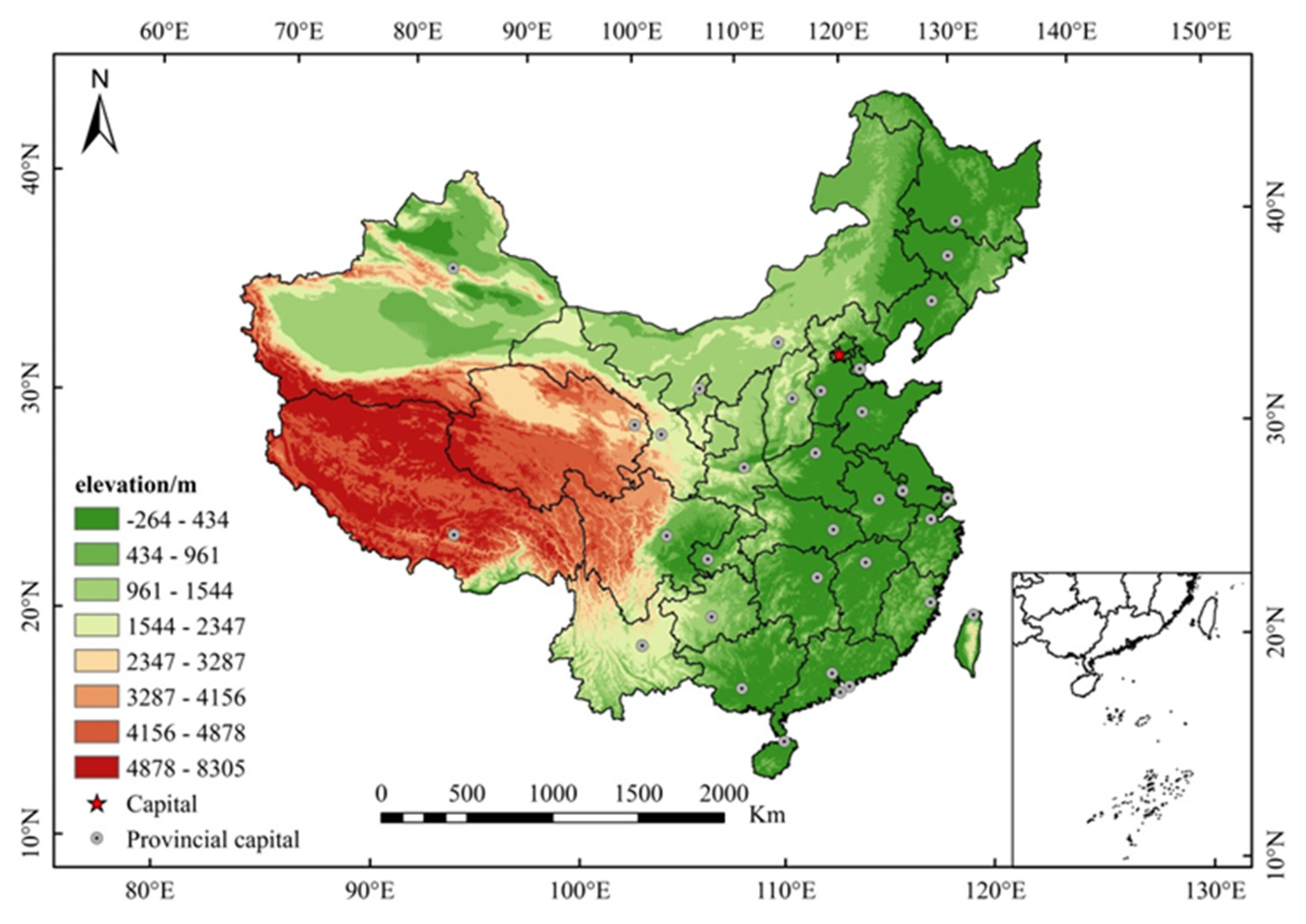
The topography of China is complex and diverse, with mountains, plateaus and hills covering 67% of the country’s total land area, and basins and plains covering 33%, with elevations ranging from negative264 to 8305 m.a.s.l. (
Figure 1). In addition, China is divided into seven geographic regions: Northeast (NE), Northwest (NW), Southwest (SW), East China (EC), Central China (CC), North China (NC), and South China (SC) according to geographic and economic characteristics. EC, CC and SC are more developed regions; NE, NC, and SW are less developed regions; and NW is the least developed region (
Figure 2).
2.2. Data Sources
Many of the techniques for deriving tropospheric ozone are based on the tropospheric ozone residual (TOR) method, which derives tropospheric column ozone (TCO) by subtracting concurrent measurements of stratospheric column ozone (SCO) from total column ozone measured by the total ozone mapping spectrometer (TOMS) instrument [
23]. The TOR concept, which has been used by Fishman et al., using both the TOMS and solar backscatter ultraviolet (SBUV) [
24], and by Chandra et al., using both the TOMS and the upper atmosphere research satellite (UARS) microwave limb sounder (MLS) [
25], has been implemented to derive TCO and SCO fields from the Aura satellite where total column ozone is measured by the Dutch–Finnish ozone monitoring instrument (OMI) [
26], and SCO is measured by the MLS instrument [
27].
The use of MLS onboard Aura for measuring SCO is a significant improvement in alleviating some of the problems associated with the use of SBUV or UARS MLS. The OMI and MLS instruments onboard the Aura spacecraft platform have been providing global measurements of total and stratospheric column ozone since soon after the launch of Aura on 15 July 2004 (
http://aura.gsfc.nasa.gov/) [
28]. This has enabled near global measurements of TCO on almost a day-to-day basis from late August 2004 to the present.
MLS and OMI are two of four instruments onboard the Aura spacecraft, which is travels in a sun-synchronous polar orbit at a n altitude of 705 km and an inclination of 98.2°. The spacecraft’s equatorial crossing time is 1:45 p.m. (ascending node) with approximately 98.8 min per orbit (an average 14.6 orbits per day) [
29].
The MLS instrument is a thermal-emission microwave limb sounder that measures vertical profiles of mesospheric, stratospheric, and upper tropospheric temperature, ozone, and other constituents from limb scans ahead of the Aura satellite. The MLS profile measurements are taken about 7 min before OMI views the same location during ascending (daytime) orbital tracks. These are referred to as “collocated” measurements between OMI and MLS. The MLS also measures ozone and other atmospheric constituents in descending nighttime orbits for a given day with a time difference of up to ±12 hours from OMI measurements, and the MLS combines ascending and descending nodes. Details regarding the instrument, including spectrometers, spectral channels, calibration, and other topics, are discussed by Waters et al., and in the same journal with related papers, there were around 3500 vertical profile measurements over the Earth per day [
27]. The MLS ozone profile measurements were interpolated to the existing NCEP tropopause pressure to derive the SCO. Measurements of MLS SCO were determined by a standard method of pressure integration of the ozone volume mixing ratio [
30]. Only the ascending orbit juxtaposition data from the MLS for the derivation of SCO are included in this study.
OMI is a nadir-scanning instrument that at visible and UV wavelength channels detects backscattered solar radiance to measure column ozone with near global coverage (aside from polar night latitudes) over the Earth with a resolution of 13 km × 24 km at nadir. Aside from ozone, OMI can also determine cloud-top pressure, aerosols and aerosol parameters, NO
2, SO
2 and other trace constituents in the troposphere and stratosphere [
26]. Total ozone from OMI is derived from the TOMS version 8 algorithm. A description of this algorithm may be obtained from the TOMS V8 CD DVD ROM, or from the OMI Algorithm Theoretical Basis Document (
https://toms.gsfc.nasa.gov/version8/v8toms_atbd) [
29].
The SCO concentration in this study comes from OMI-MLS, and the total ozone column concentration data comes from OMI-TOMS3. Available from the NASA (National Aeronautics and Space Administration) Goddard Earth Science Data and Information Service Center (GES DISC), all files are stored in the EOS layered data format, providing global coverage on a daily time scale.
Meteorological data (wind field, temperature and precipitation) were collected from “China Monthly Surface Climate Data Set” (
http://data.cma.cn/data/cdcindex/cid/6d1b5efbdcbf9a58.html), with a total of 15 years and 613 meteorological stations. The GDP (gross domestic product) kilometer grid dataset and land use and cover data were acquired from a resource and environment data cloud platform of the Chinese Academy of Sciences (
https://www.resdc.cn/DOI/DOI.aspx?DOIid=54). The GDP spatial distribution map was based on county-level statistical data closely related to anthropogenic economic activities, using multi-factor weight analysis [
31,
32]. In addition, the land use and cover map were obtained by manual visual interpretation based on Landsat TM/ETM remote sensing images. In addition, NDVI (normalized difference vegetation index) data were derived from MOD13Q1 products, and available from the MODIS satellite (
https://lpdaac.usgs.gov/products/mod13q1v006/).
2.3. Data Methodology
TCO data were acquired from the OMI product between 1 January 2005 and 31 December 2019. The data were filtered according to the transit time (4:30 to 8:30) and stored in the HDF format. VISAN software was used to extract TCO concentration, which matched with the latitude and longitude of China. In order to ensure the full coverage of the study area and to improve the accuracy of the interpolation, the data were filtered and removed with a large solar zenith angle (>70°), relatively high cloud fraction (>20%) and possible contamination due to the OMI row anomaly [
33]. Then, the processed data were stored in excel tables according to latitude and longitude. Finally, spatial kriging interpolation and mask methods were applied in ArcGIS 10.3. The average statement was input into the grid calculator to calculate the average value of one day; then the average values of month, season and year were calculated using the average value of one day. Spatiotemporal variation of TCO concentration could be analyzed by using the results obtained.
The pollutant emission data (NO
x and VOCs) were obtained from the MIX Asian Emissions Inventory is an anthropogenic source emission inventory for Asian Man-made Emissions developed by Tsinghua University [
34]. We used a multi-scale joining method through assimilation of anthropogenic emission inventories and provided monthly emission grid data with 0.25-degree spatial resolution in five emission sectors (power, industry, residents, transportation, agriculture).
The spatial correlation calculation was based on the pixel spatial analysis method, which could analyze the correlation of TCO concentration and various impact factors (temperature, precipitation and vegetation coverage). In this study, the correlation of ozone concentration combined with the above three factors were analyzed.
is the correlation coefficient between TCO concentration, temperature, precipitation and vegetation coverage; the threshold is (−1, 1). represents the average value of TCO concentration in the i-th month, represents the average value of TCO concentration in 12 months, represents the average value of impact factors (temperature, precipitation or vegetation coverage) in the i-th month, represents the 12-month average value of the impact factor, n = 12.
The HYSPLIT model was researched and developed jointly by the National Oceanic and Atmospheric Center and the Australian Meteorological Agency. This model can be used to calculate and analyze airflow movement, mass sedimentation, pollutant transport pathways and diffusion trajectories [
35,
36,
37]. TrajStat software was implemented to identify potential path sources from the long-term measurements of air pollutants [
38]. We used TrajStat software to analyze the backward trajectory of TCO. Shenyang (41°48′ N, 123°25′ E), Beijing (39°56′ N, 116°20′ E), Lanzhou (36°03′ N, 103°73′ E), Chengdu (30°67′ N, 104°07′ E), Wuhan (30°52′ N, 114°31′ E), Shanghai (31°23′ N, 121°47′ E) and Guangzhou (23°16′N, 113°23′E) were set as the simulated receiving points. The daily monitoring time was implemented at 00:00, 6:00, 12:00 and 18:00 (Beijing time) from 2019.
3. Result and Discussion
This study analyzed the annual, seasonal and monthly spatiotemporal distribution of TCO concentration over China from 2005 to 2019. We only discussed TCO in the continent. In order to more clearly reflect the distribution of TCO over China, TCO concentrations were divided into seven levels according to the natural break point classification method: first level (30–35), second level (35–40), third level (40–45), fourth level (45–50), fifth level (50–55), sixth level (55–60), seventh level (>60). Different colors represent different levels, and the unit used was the Dobson unit (DU).
3.1. Inter-Annual Variations of TCO Concentration
This study only discusses TOC concentration if not specified otherwise. To characterize the evolution of TCO spatial distribution, the maximum, minimum, and average values of ozone concentration are shown in
Figure 3. The three values of ozone concentration maintained the increasing trend from 2005 to 2010 and the declining trend after 2010. This is due to the strict control of ozone emissions during the China’s 11th Five-Year Plan (2006-2010) when the government placed more emphasis on industrial desulfurization [
39]. However, the overall trend showed a slight increase from 2014 to 2018.
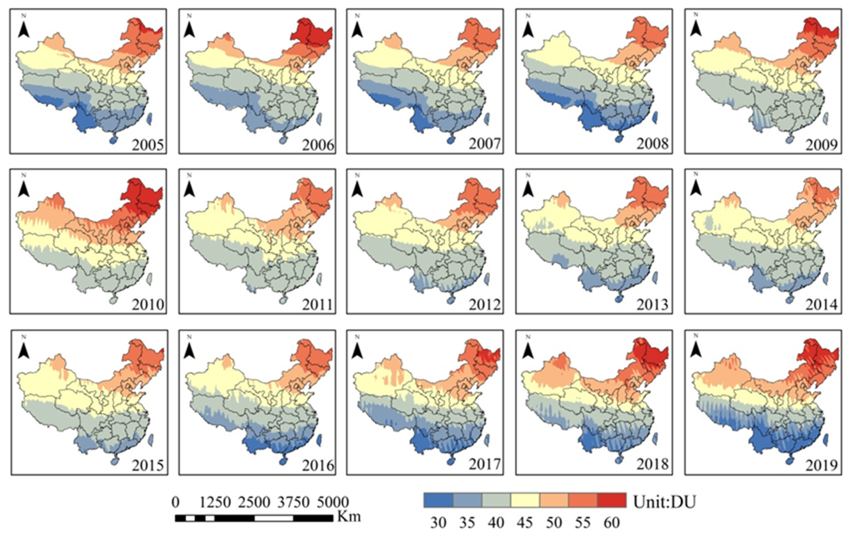
The spatial distribution of TCO concentration increased gradually from South to North China. Due to the influence of topography and climate, high values were observed in the NE region, and low values were observed in the SW region. The ozone concentration increased slowly in the first 6 years, and the high values diffused from north to south continuously, reaching the seventh level in 2006, 2009, and 2010, which was related to the increase in industrial pollution and energy consumption [
40], while the first level areas disappeared gradually. In 2013, the ozone concentration decreased and the scope of the fifth level zone continued to narrow. This was due to the new standard of air pollution control engineering that had been launched officially; the concentration of air pollutants, including ozone, decreased significantly [
40]. After 2013, ozone concentration began to decrease, followed by a rebound in 2014–2016, which may be due to the combination of ozone precursor emissions with high temperature and radiation. Moreover, low values appeared in the SW region, which represented an improvement in air quality (
Figure 4).
3.2. Seasonal Variations of TCO Concentration
The seasonal variations of TCO concentration maintained the pattern of spring > winter > summer > autumn in the past 15 years (
Figure 5). This is due to the photochemical reaction caused by the increase in solar radiation, which increased the concentration of TCO [
41]. The maximum TCO concentrations in spring, winter, summer, and autumn were 35.82 DU, 33.45 DU, 31.93 DU, and 29.96 DU, respectively. However, the trend changed from 2016 onwards. The concentration of TCO increased significantly in autumn, which was mainly due to the increase in TCO concentration caused by stratospheric ozone input due to climate change in the autumn of 2016.
Figure 6 suggests that the high TCO concentrations in spring and winter were located in NE, while the low TCO concentration areas in summer and autumn were located in SW and SC. The TCO concentration in NE was extremely high with the seventh level, the NC and CC areas were in the fourth to the sixth level, and the SW and SC areas were in the third level in spring. In summer, TCO concentration was in the range of the third to the fifth level and extended to NW and CC. By autumn, the range of the third level showed little change, while the second level of ozone appeared in SW and CC. In winter, TCO concentration increased to the seventh level in NE and the fifth and the sixth level in NC, while the concentration in CC was at the third and the fourth level. The SC and SW were at the first and second levels. The reason for the high TCO concentration in the above seasons was the strong solar radiation, which led to the transformation of ozone precursors, and the lower temperature and humidity may have weakened the ozone deposition rate [
41,
42].
3.3. Monthly Variations of TCO Concentration
It can be seen from
Figure 7 that the monthly variations of TCO concentration displayed a cyclical trend during 2005–2019. The TCO concentration was at a low value from June to November, and the lowest TCO concentration occurred in September 2006 (39.48 DU). By contrast, high TCO concentration appeared from December to May, and the highest value was in April 2010 (54.87 DU). The pattern of TCO concentration might be related to emission ozone precursors such as alkanes and olefins, which are prone to photochemical reactions under high temperature and intense radiation in spring [
2].
4. Main Influencing Factors of TCO
4.1. Influences of Natural Factors
4.1.1. Wind Field
Meteorological factors play crucial roles in the formation, conversion, transportation, and removal of ozone, all of these meteorological factors affect the concentration of TCO. The wind is one of the main means of dissemination medium for air pollution, and its intensity and direction can directly affect the speed and direction of ozone diffusion. Stable high-pressure fields are the main weather systems that form heavy pollution at medium or large scales [
43]. The direction of prevailing wind in winter is northwest wind influenced by Siberian high pressure. The dominant wind in summer was southeast wind, which is due to the high temperature, rapid warming, and low air pressure in the Eurasian continent. Spring and autumn are the transitional periods of the northeast and southeast monsoon. Ozone concentration is lower in summer when the southeast monsoon prevails since the wind from the sea brings much more clean air, which is favorable for the diffusion of ozone pollutants. The spatial pattern of ozone concentration showed that the northern area was higher than the southern area in China under the influence of the dominant wind (
Figure 8).
4.1.2. Temperature and Precipitation
Figure 9 shows the correlation between annual average TCO concentration and temperature from 2005 to 2019. The average correlation coefficient R
1 is 0.51, and the area positively correlated was about 38.40% in the total area. Moreover, TCO concentration was positively correlated with temperature in the NE, CC and SC regions (correlation coefficient above 0.4). When the temperature rises, the production rate of ozone accelerates under the double influence of heat and strong oxidation reactions [
6].
Figure 10 shows the correlation between annual TCO concentration and precipitation from 2005 to 2019. A total of 42.60% of the area was negatively correlated with TCO concentration (correlation coefficient R
2 = −0.36). This was due to the increase in precipitation, which is conducive to the removal of pollutants (especially ozone) [
44]. The concentration highly correlated with precipitation was in NW and EC, with a correlation coefficient above 0.4. This was due to the simultaneous increase in temperature and precipitation in summer in these regions, especially in the NW, which was concentrated in summer.
4.1.3. Vegetation Coverage
Vegetation can change the stability of the carbon cycle and climate system, which plays a role in energy flow and the material cycle in the ecosystem [
45].
Figure 11 shows the correlation between annual TCO concentration and vegetation coverage from 2005 to 2019, of which 42.10% was negatively correlated and 57.9% was positively correlated. Isoprene, as the largest volatile organic compound emitted by plants, had a significant contribution to the production of ozone [
46]. EC is close to the sea, rich in water vapor, and diverse in vegetation, which mainly consists of distributed deciduous broad-leaved forests and evergreen broad-leaved forests. Large amounts of VOCs released by plants provide precursors for photochemical reactions and then are transported to cities with the wind, which leads to higher TCO concentrations. Comparatively, the Gobi and desert areas in NW are influenced by arid climate, sparse vegetation, and low isoprene emission, so correlation coefficient was lower.
4.2. Influences of Anthropogenic Factors
4.2.1. Spatial Distribution of GDP
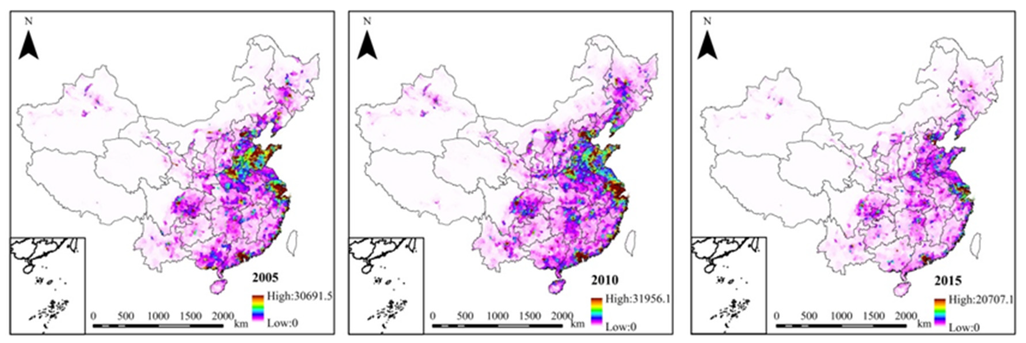
GDP is an important indicator index of social-economic development, regional planning, and environmental protection.
Figure 12 shows that the GDP in 2005, 2010, and 2015 was 306.915, 319.561, and 207.071 million Yuan /km
2, while the TCO concentration was 38.26, 40.32, and 25.87 DU. The change of TCO was closely related to the development of the secondary industry. As the pillar industries of the secondary industry, the petroleum and chemical industries produced large amounts of precursors in the atmosphere, which could ultimately have affected ozone concentration [
43]. In addition, due to the large usage of agricultural equipment and vehicles with the development of agriculture and tourism, more exhaust gases are generated, which could lead to an increase in TCO concentration [
47].
4.2.2. Emissions of NOx and VOCs
NO
x and VOCs were produced in the processes of coal combustion, automobile exhaust and the heavy chemical industry. NO
x and VOCs are precursors of ozone [
41]. In order to analyze the impact of different types of emission sources on TCO, this paper combined the MIX emission list from seven geographical divisions.
Rapid industrial development could affect NO
x emissions from different sources in different regions (
Table 1). As EC and NC were the gathering places of China’s heavy industry, the industries in EC and NC made a great contribution to NO
x emission, accounting for 31.73% and 17.85% of China’s NO
x emission, respectively. NE and SC account for 7.31% and 8.02%, respectively, which is due to slow industrial development and low NO
x emission. The power sector was the main reason for the decline in NO
x (contribution percentage > 30%). In addition, industrial sources and traffic sources were other factors responsible for NO
x emission, with a contribution rate of more than 25%.
VOCs, another important source of TCO, have become the main precursors that may gradually influence the changes in TCO concentrations in recent years.
Table 2 shows that industries in EC contributed significantly and that the emission rate of VOCs accounted for 39.20%. Residential and traffic sources were the other two main sources. The rapid development of industry and the increase in population in EC led to the increase in VOC emissions, while the slow industrial development and a small population in NW and SW led to low VOC emissions. The contribution rate of power sources was less than 2% compared with other sources, indicating that VOCs emitted by power stations had a weaker effect.
4.3. Clustering of Backward Air Trajectories
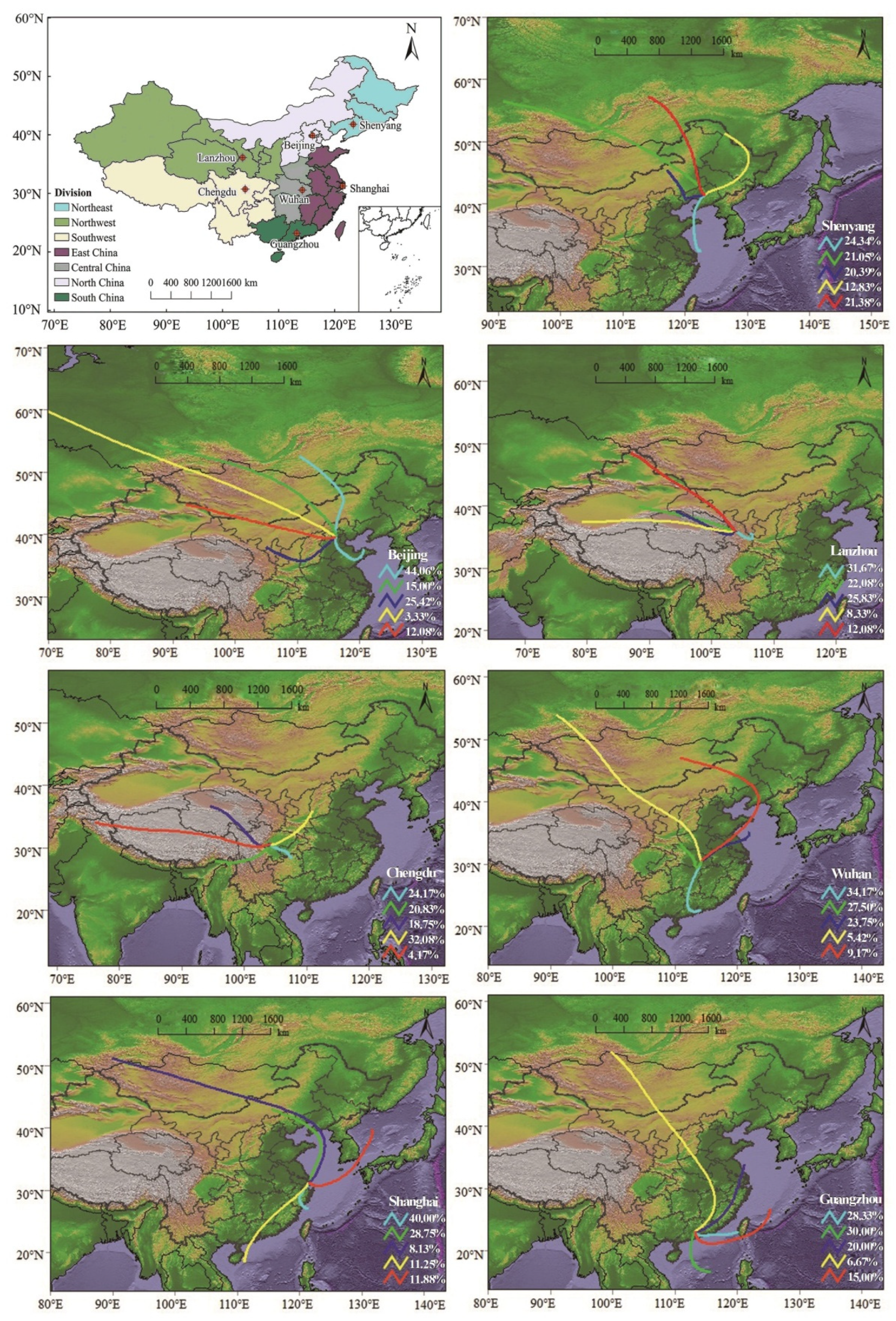
Figure 13 shows the cluster of the airflow backward trajectory in seven typical cities from 2005 to 2019 to reflect the characteristics of the airflow. Each complete path represented a different backward airflow path. A total of five main paths and the ratio of each path were obtained. The northwest airflow in cities in NC (Shenyang, Beijing, and Lanzhou) had the fastest moving speed and the longest transport distance. In addition, the airflow trajectory proportions of the above cities were 42.43%, 59.06%, and 37.91%, respectively, while the airflow moved slowly in East and South China and the transportation distance was short. Except for northwest airflow, southern and southeast airflow gradually increased in cities in SC (Chengdu, Wuhan, Shanghai, and Guangzhou), accounting for 24.17%, 34.17%, 40.00%, and 45.00% (
Table 3), respectively, especially in Shanghai and Guangzhou, where airflow deriving from the ocean was frequent. The northwest airflow originated in the Gobi Desert region (The Gobi Desert is a vast, arid region in northwestern China.). For example, the Taklamakan Desert is the most important long range path for transport of TCO.. The medium-distance paths passed through the Northeast Plain, the North China Plain, the middle and lower plain of the Yangtze River, while the short-distance airflows originated from coastal cities in low-altitude regions with dense populations and fragile ecologies. In general, airflow with prevailing northwest winds in winter and southeast winds in summer resulted in higher TCO concentrations, while other airflow paths corresponded to lower TCO concentrations.
5. Conclusions
The spatiotemporal variation of TCO concentration from 2005 to 2019 in China was derived from OMI data. The results showed that China had an imbalanced spatial distribution of TCO concentration in 2005–2019, with high values distributed in the NE region in 2010 and low values observed in the SC region in 2019. The TCO concentration during different seasons maintainedthe same pattern: spring’s concentration is greater than winter’s concentration, winter’s concentration is greater than summer’s concentration, summer’s concentration is greater than autumn’s concentration. In addition, TCO had a low concentration from June to November and a high concentration from December to May. Regarding natural factors, TCO concentration was positively correlated with wind field, temperature, and partial vegetation coverage, while precipitation had a negative effect on TCO concentration. Regarding anthropogenic factors, the inherent mechanism of the TCO’s spatiotemporal pattern of TCO might be the human socio-economic activities such as land use and cover changes. The emission of NOx and VOCs was the main reason for the increase in TCO concentration. The backward trajectory and cluster analysis revealed that northwest and southeast airflows led to high ozone concentrations.
On the whole, the influent mechanism of TCO was complicated, and both natural and anthropogenic factors played important roles. This study recommends more long-term remote sensing monitoring and implementation of control strategies, which are essential to safeguard the health of people, the ecosystem, and the climate. The key measure for accomplishing the reduction in TCO concentration is to restructure energy sources by reducing coal consumption, vigorously developing clean energy, and increasing the usage of hydropower, wind power, and solar power. It is also essential to monitor ozone pollution effectively in the urbanization of China.
Author Contributions
Methodology, software and formal analysis, L.Z.; writing—review and editing, M.L.; investigation, data curation and writing—original draft preparation, J.S. All authors have read and agreed to the published version of the manuscript.
Funding
This research was funded by the National Natural Science Foundation of China (31760135), the Gansu Provincial Natural Science Foundation (20JR10RA089) and the Gansu Provincial Forestry and Grassland Science and Technology Innovation (KJCX2021005).
Institutional Review Board Statement
Not applicable.
Informed Consent Statement
Not applicable.
Data Availability Statement
Acknowledgments
We thank the NASA Earth System for OMI/Aura Level-2 O
3 data used in this study, which were acquired at
http://disc.sci.gsfc.nasa.gov/, and the Chinese Academy of Sciences for sharing the China Statistical Bureau. (accessed on 6 July 2020).
Conflicts of Interest
All the authors do not have any possible conflicts of interest.
References
- Kondratyev, K.Y.; Varotsos, C. Atmospheric greenhouse effect in the context of global climate change. IL Nuovo Cim. 1995, 18, 123–151. [Google Scholar] [CrossRef]
- Hu, Y.M.; Yan, H.H.; Zhang, X.Y.; Gao, Y.; Zheng, X.D.; Liu, X.Y. Study on calculation and validation of tropospheric ozone by ozone monitoring instrument–microwave limb sounder over China. Int. J. Remote Sens. 2020, 41, 9101–9120. [Google Scholar] [CrossRef]
- World Meteorological Organization (WMO). Scientific Assessment of Ozone Depletion Global Ozone Research and Monitoring Project; Report No. 52, 516; World Meteorological Organization: Geneva, Switzerland, 2010. [Google Scholar]
- Chen, X.; Zhong, Q.B.; Huang, X.F.; Wang, X.M.; Sarkar, S.; Jia, S.G.; Deng, X.J.; Chen, D.H.; Shao, M. The role of natural factors in constraining long-term tropospheric ozone trends over southern China. Atmos. Environ. 2020, 220, 117060. [Google Scholar] [CrossRef]
- Moortgat, G.K. Important photochemical processes in the atmosphere. Pure Appl. Chem. 2001, 73, 487–490. [Google Scholar] [CrossRef][Green Version]
- Xu, J.; He, Y.J.; Li, M.Z.; Zhang, Z.Z.; Du, X.H.; Wang, J.K.; Yang, X.; Wu, Z.H.; Li, H.; Chen, Y.Z.; et al. A high ozone event over Beijing after the May 2017 Belt and Road Forum. Atmos. Pollut. Res. 2021, 12, 287–297. [Google Scholar] [CrossRef]
- Kvalevåg, M.M.; Myhre, G. Human Impact on Direct and Diffuse Solar Radiation during the Industrial Era. J. Clim. 2007, 20, 4874–4883. [Google Scholar] [CrossRef]
- Ge, S.J.; Wang, S.J.; Xu, Q.; Ho, T. Effect of Dynamic Low DREs from Flare Combustion on Regional Ozone Pollution during A Chemical Plant Shutdown. Atmos. Environ. 2021, 254 Pt A, 118399. [Google Scholar] [CrossRef]
- Cheng, M.M.; Jiang, H.; Guo, Z.; Zhang, X.M.; Chen, J. Correlation between the spatio-temporal distributions of aerosols, sulphur dioxide, and formaldehyde using MODIS and SCIAMACHY satellite data for China. Int. J. Remote Sens. 2015, 36, 3961–3978. [Google Scholar] [CrossRef]
- Sitnov, S.A.; Mokhov, I.I. Formaldehyde and nitrogen dioxide in the atmosphere during summer weather extremes and wildfires in European Russia in 2010 and Western Siberia in 2012. Int. J. Remote Sens. 2017, 38, 4086–4106. [Google Scholar] [CrossRef]
- Miatselskaya, N.; Kabashnikov, V. The possibility of using an optical gas filter method for remote sounding of the total atmospheric column of SO2. Int. J. Remote Sens. 2011, 32, 3079–3092. [Google Scholar] [CrossRef]
- Jiang, J.; Zha, Y.; Gao, J.; Jiang, J.J. Monitoring of SO2 column concentration change over China from Aura OMI data. Int. J. Remote Sens. 2012, 33, 1934–1942. [Google Scholar] [CrossRef]
- Thomas, H.E.; Watson, I.M.; Carn, S.A.; Prata, A.J.; Realmuto, V.J. A comparison of AIRS, MODIS and OMI sulphur dioxide retrievals in volcanic clouds. Geomat. Nat. Hazards Risk 2011, 2, 217–323. [Google Scholar] [CrossRef]
- Liu, Q.; Ding, W.D.; Fu, Y.F. The seasonal variations of aerosols over East Asia as jointly inferred from MODIS and OMI. Atmos. Ocean. Sci. Lett. 2011, 4, 330–337. [Google Scholar]
- Thomas, A.J.; Sundar, A.C. A multi-sensor approach for assessing the impacts of ultraviolet-absorbing aerosols on top of atmosphere radiative fluxes. Int. J. Remote Sens. 2011, 32, 4659–4682. [Google Scholar]
- Zhang, J.; Van Der, A.R.J.; Ding, J.Y. Detection and emission estimates of NOx sources over China North Plain using OMI observations. Int. J. Remote Sens. 2018, 39, 2847–2859. [Google Scholar] [CrossRef]
- Xu, C.; Wang, Y.P.; Li, L.L. Study on spatiotemporal distribution of the tropospheric NO2 column concentration in China and its relationship to energy consumption based on the time-series data from 2005 to 2013. Energy Sources Part A Recovery Util. Environ. Eff. 2019, 42, 2130–2144. [Google Scholar] [CrossRef]
- Finlayson-Pitts, B.J.; Pitts, J.N., Jr. Atmospheric Chemistry of Tropospheric Ozone Formation: Scientific and Regulatory Implications. Air Waste Manag. Assoc. 1993, 43, 1091–1100. [Google Scholar] [CrossRef]
- Tarasick, D.W.; Slater, R. Ozone in the troposphere: Measurements, climatology, budget, and trends. Atmosphere-Ocean 2008, 46, 93–115. [Google Scholar] [CrossRef]
- Lee, Y.C.; Shindell, D.T.; Faluvegi, G.; Wenig, M.; Lam, Y.F.; Ning, Z.; Hao, S.; Lai, C.S. Increase of ozone concentrations, its temperature sensitivity and the precursorfactor in South China. Tellus B Chem. Phys. Meteorol. 2014, 66, 23455. [Google Scholar] [CrossRef]
- Zhao, Z.; Zhou, Z.; Russo, A. Impact of meteorological conditions at multiple scales on ozone concentration in the Yangtze River Delta. Environ. Sci. Pollut. Res. 2021, 28, 62991–63007. [Google Scholar] [CrossRef]
- Chen, D.M.; Feng, Y.; Zhang, X.Y. Comparison of variability and change rate in tropospheric NO2 column obtained from satellite products across China during 1997–2015. Int. J. Digit. Earth 2017, 10, 814–828. [Google Scholar] [CrossRef]
- Fishman, J.; Watson, C.E.; Larsen, J.C.; Logan, J.A. Distribution of tropospheric ozone determined from satellite data. J. Geophys. Res. 1990, 95, 3599–3617. [Google Scholar] [CrossRef]
- Fishman, J.; Wozniak, A.E.; Creilson, J.K. Global distribution of tropospheric ozone from satellite measurements using the empirically corrected tropospheric ozone residual technique: Identification of the regional aspects of air pollution. Atmos. Chem. Phys. 2003, 3, 893–907. [Google Scholar] [CrossRef]
- Chandra, S.; Ziemke, J.R.; Martin, R.V. Tropospheric ozone at tropical and middle latitudes derived from TOMS/MLS residual: Com parison with a global model. J. Geophys. Res. Atmos. 2003, 108, 4291. [Google Scholar] [CrossRef]
- Levelt, P.F.; Hilsenrath, E.; Leppelmeier, G.W.; Oord, G.; Veefkind, J.P. Science objectives of the Ozone Monitoring Instrument. IEEE Trans. Geosci. Remote Sens. 2006, 44, 1199–1208. [Google Scholar] [CrossRef]
- Waters, J.W.; Froidevaux, L.; Harwood, R.S.; Jarnot, R.F.; Pickett, H.M.; Read, W.G.; Siegel, P.H.; Cofield, R.E.; Filipiak, M.J. The Earth Observing System Microwave Limb Sounder (EOS MLS) on the Aura satellite. IEEE Trans. Geosci. Remote Sens. 2006, 44, 1075–1092. [Google Scholar] [CrossRef]
- Schoeberl, M.R.; Duncan, B.N.; Douglass, A.R.; Waters, J.; Livesey, N.; Read, W.; Filipiak, M. The carbon monoxide tape recorder. Geophys. Res. Lett. 2006, 33, L12811. [Google Scholar] [CrossRef]
- Ziemke, J.R.; Chandra, S.; Duncan, B.N.; Froidevaux, L.; Bhartia, P.K.; Levelt, P.F.; Waters, J.W. Tropospheric ozone determined from Aura OMI and MLS: Evaluation of measurements and comparison with the Global Modeling Initiatives Chemical Transport Model. J. Geophys. Res. 2006, 111, D19303. [Google Scholar] [CrossRef]
- Froidevaux, L.; Livesey, N.J.; Read, W.G.; Jiang, Y.B.; Jimenez, C.; Filipiak, M.J.; Schwartz, M.J.; Santee, M.L.; Pumphrey, H.C.; Jiang, J.H. Early validation analyses of atmospheric profiles from EOS MLS on the Aura satellite. IEEE Trans. Geosci. Remote Sens. 2006, 44, 1075–1092. [Google Scholar] [CrossRef]
- Ling, Y.I.; Xiong, L.Y.; Yang, X.H. Method of Pixelizing GDP Data Based on the GIS. J. Gansu Sci. 2006, 2, 54–58. [Google Scholar]
- Xu, X.L. China’s GDP Spatial Distribution Kilometers Grid Dataset; Data Registration and Publishing System of the Resource and Environmental Science Data Center in the Chinese Academy of Sciences: Beijing, China, 2017. [Google Scholar]
- Witte, J.C.; Schoeberl, M.R.; Douglass, A.R.; Gleason, J.F.; Krotkov, N.A.; Gille, J.C.; Pickering, K.E.; Livesey, N. Satellite observations of changes in air quality during the 2008 Beijing Olympics and Paralympics. Geophys. Res. Lett. 2009, 36, 1–6. [Google Scholar] [CrossRef]
- Li, M.; Zhang, Q.; Kurokawa, J.; Woo, J.H.; He, K.; Lu, Z.F.; Ohara, T.; Song, Y.; Streets, D.G.; Carmichael, G.R. MIX: A mosaic Asian anthropogenic emission inventory under the international collaboration framework of the MICS-Asia and HTAP. Atmos. Chem. Phys. 2017, 17, 935–963. [Google Scholar] [CrossRef]
- Salmabadi, H.; Khalidy, R.; Saeedi, M. Transport routes and potential source regions of the Middle Eastern dust over Ahvaz during 2005–2017. Atmos. Res. 2019, 241, 104947. [Google Scholar] [CrossRef]
- Draxler, R.R.; Hess, G.D. An overview of the hysplit-4 modeling system for trajectories. Aust. Meteorol. Mag. 1998, 47, 295–308. [Google Scholar]
- Stein, A.F.; Draxler, R.R.; Rolph, G.D.; Stunder, B.J.B.; Cohen, M.D.; Ngan, F. NOAA’s HYSPLIT atmospheric transport and dispersion modeling system. Bull. Am. Meteorol. Soc. 2016, 96, 2059–2077. [Google Scholar] [CrossRef]
- Wang, Y.Q.; Zhang, X.Y.; Draxler, R.R. TrajStat: GIS-based software that uses various trajectory statistical analysis methods to identify potential sources from long-term air pollution measurement data. Environ. Model. Softw. 2009, 24, 938–939. [Google Scholar] [CrossRef]
- Gao, C.; Xiu, A.J.; Zhang, X.L.; Chen, W.W.; Liu, Y.; Zhao, H.M.; Zhang, S.C. Spatiotemporal characteristics of ozone pollution and policy implications inNortheast China. Atmos. Pollut. Res. 2020, 11, 357–369. [Google Scholar] [CrossRef]
- Ministry of Ecology and Environment of the People’s Republic of China. Bulletin on the State of China’s Ecological Environment; Ministry of Ecology and Environment of the People’s Republic of China: Beijing, China, 2019.
- Song, J.Y.; Liu, M.X.; Sun, R.D.; Li, Q.D.; Zhang, Y.Y.; Li, B.W. Temporal and spatial characteristics of atmospheric ozone concentration in Southeast Coast based on OMI data. Acta Sci. Circumstantiae 2020, 40, 438–449. [Google Scholar]
- Wang, Z.S.; Lv, J.G.; Tan, Y.F.; Guo, M.; Gu, Y.Y.; Xu, S.; Zhou, Y.H. Temporospatial variations and Spearman correlation analysis of ozone concentrations to nitrogen dioxide, sulfurdioxide, particulate matters and carbon monoxide in ambient air, China. Atmos. Pollut. Res. 2019, 10, 1203–1210. [Google Scholar] [CrossRef]
- Su, X.Q.; An, J.L.; Zhang, Y.X.; Zhu, P.; Zhu, B. Prediction of ozone hourly concentrations by support vector machine and kernel extreme learning machine using wavelet transformation and partial least squares methods. Atmos. Pollut. Res. 2020, 11, 51–60. [Google Scholar] [CrossRef]
- Xue, R.B.; Wang, S.S.; Li, D.R.; Zou, Z.; Chan, K.L.; Valks, P.; Saiz-Lopez, A.; Zhou, B. Spatio-temporal variations in NO2 and SO2 over Shanghai and Chongming Eco-Island measured by Ozone Monitoring Instrument (OMI) during 2008–2017. J. Clean. Prod. 2020, 258, 120563. [Google Scholar] [CrossRef]
- Fan, J.C.; Ju, T.Z.; Wang, Q.H.; Gao, H.Y.; Hu, R.R.; Duan, J.L. Spatiotemporal variations and potential sources of tropospheric formaldehyde over eastern China based on OMI satellite data. Atmos. Pollut. Res. 2021, 12, 272–285. [Google Scholar] [CrossRef]
- Weiss, J.L.; Gutzler, D.S.; Coonrod, J.E.A.; Dahm, C.N. Seasonal and inter-annual relationships between vegetation and climate in central New Mexico, USA. J. Arid. Environ. 2004, 57, 507–534. [Google Scholar] [CrossRef]
- Mo, Y.P.; Karimian, H.; Zhang, S.T.; Kong, X.Y.; Fang, S.W.; Tang, B.Y. Daily spatiotemporal prediction of surface ozone at the national level in China: An improvement of CAMS ozone product. Atmos. Pollut. Res. 2020, 12, 391–402. [Google Scholar] [CrossRef]
| Publisher’s Note: MDPI stays neutral with regard to jurisdictional claims in published maps and institutional affiliations. |
© 2022 by the authors. Licensee MDPI, Basel, Switzerland. This article is an open access article distributed under the terms and conditions of the Creative Commons Attribution (CC BY) license (https://creativecommons.org/licenses/by/4.0/).


