Abstract
Future changes in drought characteristics in Central Asia are projected at the regional scale using 21 climate models from phase 5 of the Coupled Model Intercomparison Project (CMIP5). Based on the standardized precipitation index (SPI) and standardized precipitation evapotranspiration index (SPEI), drought characteristics were characterized by drought frequency at 1-, 3-, and 12-month timescales. The drought duration was analyzed based on SPI1 and SPEI1. Drought indices were calculated by the multimodel ensemble (MME) from 21 CMIP5 models. The varimax rotation method was used to identify drought conditions for the entire area and seven drought subregions. In general, the projection results of future drought in Central Asia are related to the choice of drought index, and SPI and SPEI show different results. The drought frequency based on SPEI1, SPEI3, and SPEI12 showed an increasing trend in the future periods, that is, the drought frequency based on monthly, seasonal, and annual timescales will show an increase trend in the future periods. However, for SPI1, SPI3, and SPI12, the drought frequency will decrease in the future. SPI projected that the duration of drought will decrease in the future, while SPEI mainly showed an increasing trend. The results of the study should be of sufficient concern to policymakers to avoid land degradation, crop loss, water resource deficit, and economic loss.
1. Introduction
With the development of global warming, the frequency, average duration, and severity of drought events have shown an upward trend [1]. Drought is a serious environmental phenomenon which damages agricultural production, human activity, and living space for animals and plants. Global climate warming is causing the world to become hotter and parched [2]. Climate warming has exacerbated drought in some areas. As a result, losses from drought are increasing. Especially in arid and semihumid areas, climate change and the increase of human activities are likely to lead to ecological degradation and even serious ecological and economic losses [3]. The prediction of future drought in Central Asia is of great significance in dealing with climate change [4].
Although the main reason of drought is water scarcity, other factors, such as temperature, wind speed, and soil moisture, also cause drought. Although many variables are important in drought-related processes, few observations are available in Central Asia. To study drought, various drought indices have been proposed for monitoring drought conditions. Drought indices are also widely used to project future droughts caused by climate change. To accurately monitor and evaluate the current situation or predict future droughts, it is undoubtedly important to select an appropriate drought index for each type of drought. Using different drought indices will result in different monitoring or forecasting results. Therefore, it is necessary to select a suitable drought index to evaluate the impact of drought, especially in regional studies [5].
It is well known that predicting future drought scenarios and developing effective measures are key to drought risk management in a region [6,7]. Both quantitative and qualitative drought prediction are key to drought risk management [8]. Many studies have used global climate models to project the occurrence, intensity, duration, and area of droughts at regional or global scales. The CMIP has been used to project future temperature, precipitation, and climatological drought at global and regional scales [9,10,11,12]. Some studies using the CMIP3 model suggest that frequency and intensity of droughts will increase in the future [13,14,15]. Additionally, many studies are based on CMIP5 data to calculate the drought index and analyze the characteristics of future climate change. Three drought indices (Palmer Drought Severity Index, PDSI; Standardized Precipitation Evapotranspiration Index, SPEI; Standardized Precipitation Index, SPI), based on 13 CMIP5 general circulation models (GCMs) under three representative concentration pathway scenarios are used to project the future drought characteristics in humid subtropical basins in China [16]. At the global and regional scale, SPEI is widely used in drought monitoring and prediction [17,18,19]. PDSI is considered to be only suitable for monitoring agricultural drought [20], because it has several limitations such as fixed timescale, strong dependency on the data calibration, shortcomings in spatial comparability, and arbitrary interpretation of drought conditions with the index values [21,22]. SPI has several advantages, such as multiple timescales, simple calculation, and good adaptability to different climates. In this study, drought characteristics are quantified by SPI and SPEI.
The aim of this paper is to comprehensively study the spatiotemporal drought characteristics based on CMIP5 model outputs from 2006 to 2100. Specifically, the objectives of this study are (1) to identify the subregions with distinct drought characteristics by using the Varimax rotation method; (2) to evaluate the performance of CMIP5 simulation and bias correction in Central Asia; (3) to project future drought frequency and duration; (4) to check the drought trend based on Dunnett’s multiple comparisons.
2. Data and Methods
2.1. Study Area
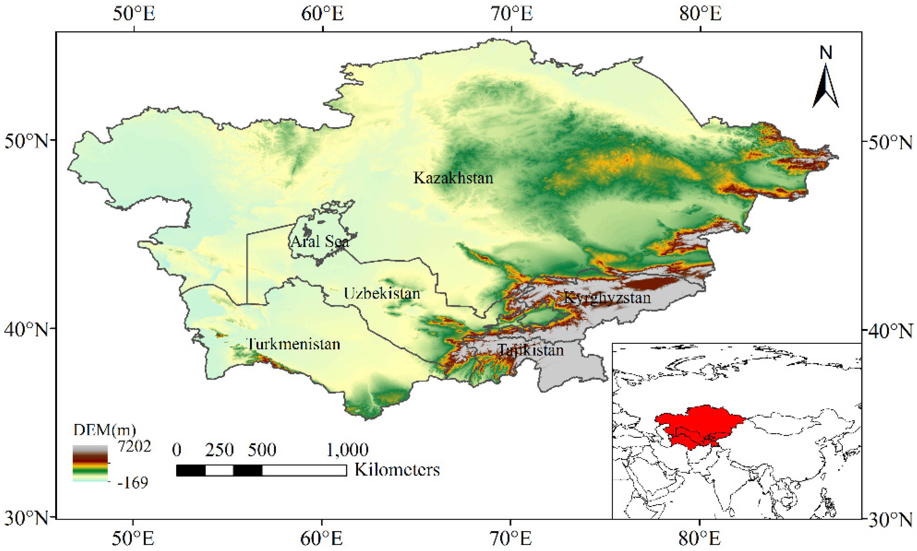
The study area is Central Asia, including five countries, Tajikistan, Kyrgyzstan, Uzbekistan, Kazakhstan, and Turkmenistan (Figure 1). Central Asia lies in the south of Russia, west of China, north of Afghanistan and Iran, and east of the Caspian Sea. Central Asia is located in arid and semiarid regions, and its ecological system is dominated by desert, so its ecological environment is relatively fragile. It belongs to the typical continental climate of temperate desert and grassland. In general, the climate is affected by the westerly circulation and the North Atlantic oscillation, which is significantly different from the East Asia region controlled by the monsoon circulation. The topography of this region is characterized by the west plateau land to east plain and hilly land. There are the Altai Mountains and Tianshan Mountains in the east, and plains and hills in the middle and west. Central Asia covers an area of about 4 million km2 and has a population of 65 million [23].
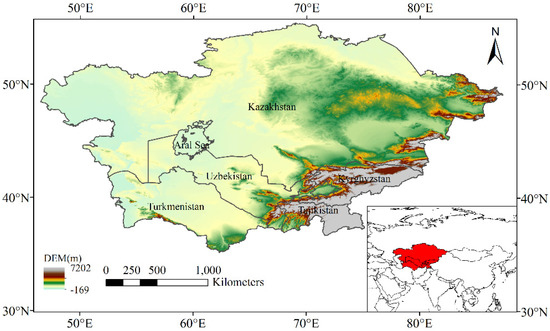
Figure 1.
Study area including five states in Central Asia.
2.2. Data
The monthly gridded observed data, such as precipitation, maximum temperature, and minimum temperature, were obtained from the Climatic Research Unit (CRU TS v4.01).
To project the characteristics of future drought changes, monthly outputs from 21 climate models were obtained from global climate models. In this study, the representative concentration pathway (RCP) 4.5 [24] was applied as the scenarios and projects the changes of drought characteristics in the 21st century. In this scenario, RCP 4.5 was the intermediate stable path; the total radiative forcing stabilized to 4.5 Wm−2, and the concentration of greenhouse gases would stabilize to 650 ppm CO2 after 2100. A total of 21 climate models were selected to provide monthly precipitation and minimum and maximum temperature data from global climate models (Table 1). The monthly data for historical (1986–2005) and future (2006–2100) periods were supported by the Climate Model Diagnosis and Intercomparison (PCMDI).

Table 1.
The information of 21 climate models used in this study.
2.3. Methods
2.3.1. Quantile Mapping
Nonparametric quantile mapping was chosen to perform the bias correction. Daily data of precipitation, minimum temperature, and maximum temperature were aggregated to monthly data. Then, the nonparametric mapping method was used to complete bias correction. The nonparametric method has a better effect on bias correction than the parametric method, because it uses the actual distribution of the observed and simulated data [25]. This method has been widely used to downscale and correct regional climate models [26,27,28,29]. The quantile mapping was performed using the Quantile mapping package in R software.
2.3.2. Rotated Empirical Orthogonal Function (REOF)
Empirical orthogonal function (EOF) can decompose the spatiotemporal field of various irregularly distributed meteorological fields, and the decomposed feature vectors are orthogonal to each other [30]. Different spatial modes can well reflect the spatial distribution characteristics of the spatiotemporal field of meteorological elements. Moreover, the expansion and convergence speed of EOF decomposition are very fast, and the information of variable field can be easily concentrated on the first few modes. The first few modes with cumulative variance contribution rate reaching a certain degree have certain physical significance, which can effectively reflect the variation characteristics of temporal and spatial field of meteorological elements. The details of empirical orthogonal function are the following:
where Z(x, y, t) is the spatial–temporal field, PC is the principal time vectors, and EOF is the principal loading field.
In this study, the Varimax-EOF, an REOF method, was used to handle variable field SPEI. The rotated loading patterns (REOFs) and rotated time coefficients (RPCs) could be obtained based on the REOF analysis. Based on the EOF decomposition of the spatial–temporal vector field, REOF decomposition is used to rotate the maximum variance (orthogonal rotation) of the original matrix, so that the high load vector field under the same spatial mode is concentrated in a few variables in some regions, and the other regions are close to 0. After rotation, the characteristic field is more stable in temporal, and the spatial distribution structure is clearer. Moreover, it is important to highlight the local characteristics of the spatial abnormal distribution of climate elements.
2.3.3. Drought Indices
In order to quantify drought, it is particularly important to choose an appropriate drought index, because there are many sources of uncertainty in predicting future droughts, such as climate model uncertainty, future scenario uncertainty, drought index uncertainty, and drought threshold uncertainty [31]. Among them, choosing a suitable drought index is the most important factor influencing the uncertainty of future drought assessment. In this study, we chose SPI and SPEI as drought indictors. SPI is the recommended index for universal meteorological drought by the World Meteorological Organization [32]. Based on the gamma distribution, we calculated the SPI1, SPI3, and SPI12. The calculation of SPEI is based on the difference between precipitation (P) and potential evapotranspiration (PET) [33]. The PET was calculated using the Penman–Monteith method, which has a more physically robust calculation process [34] and is recommended by the United Nations Food and Agriculture Organization (FAO) as the sole standard method to calculate PET. In this study, we used the log-logistic distribution in the calculation of SPEI1, SPEI3, and SPEI12. The following is the Penman–Monteith equation:
where Δ is the slope of the vapor pressure curve, Rn is monthly net radiation, G is the soil heat flux, U2 is the monthly mean wind speed at 2 m above the ground surface, γ is the psychometric constant, T is the monthly mean temperature (°C), es is the saturation vapor pressure at a given air temperature, and Rh is the monthly mean relative humidity (%).
The SPEI and SPI were calculated by using SPEI and SPI package in R software. The drought index classifications were listed in Table 1. Only severe and extreme droughts were considered (Table 2).
Table 2.
Drought index classifications for SPI and SPEI.
2.3.4. Frequency of Drought
In this study, we defined the severe drought or extreme drought as a drought event. Drought frequency is defined as the ratio of severe or extreme drought months to total drought months over a 30-year period. The drought frequency is calculated for each drought index, drought scale, and drought subregion. The drought frequency is also calculated from the historical period to the future period. The historical period refers to 1986 to 2005, and the future period is divided into 66 30-year periods from 2006 to 2100. The first 30-year period is 2006–2035, the second 30-year period is 2007–2036, and the last 30-year period is 2071–2100. The drought frequency can be formulated as
where ns is number of severe or extreme drought (drought index ≤ −1.5) months, Ns is total number of months for the study period, and s is the sequence number of grid cell.
2.3.5. Average Drought Duration
The average drought duration is defined as the ratio of the total number of severe or extreme drought months to the number of drought events in a 30-year period. Among them, one drought event is a continuous occurrence of drought. The average drought duration can be formulated as
where n is number of severe or extreme drought (drought index ≤ −1.5) months and N is total number of drought events in 30-year period.
3. Results
3.1. The Regional Division of Drought
In this study, the SPEI was employed as a criterion for drought classification. Combined with the REOF method, seven spatially well-defined subregions (SR) in CA were identified and the characteristics of drought in each subregion was analyzed.
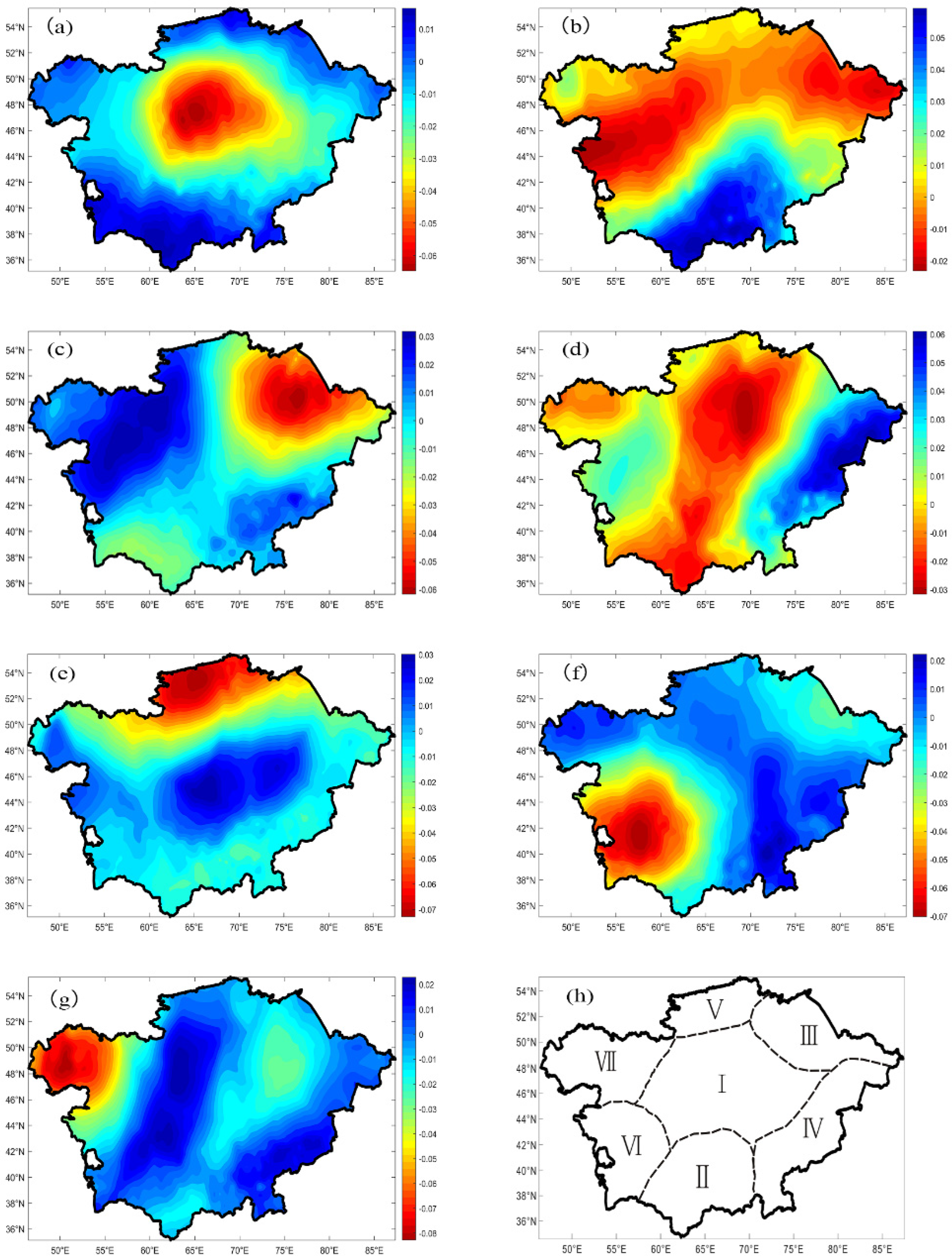
Figure 2 shows the REOF analysis results of SPEI observed by CRU on a 3-month time scale. The first seven loadings show the most dominant patterns over Central Asia (Figure 2h). The accumulative variance contribution of the first seven loadings was 65.6% of the total variance. Therefore, it can be seen that the first seven loadings dominate drought subregions over Central Asia. For SR1, the highest loadings were located in the central of Kazakhstan (Figure 2a); the variance contribution of this subregion is 26.1% of the total variance. SR2 (Figure 2b) explains approximately 13.2% of the total variance, showing the highest loadings in the southern part of Central Asia. SR3 (Figure 2c) explains about 7.6% of the total variance, with its highest loadings in northeastern Kazakhstan. SR4 (Figure 2d) explains approximately 5.3% of the total variance, and its highest loadings are in the eastern part of Central Asia, including Kyrgyzstan and Tajikistan. For SR5 (Figure 2e), the highest loadings are located in the northern part of Kazakhstan, which explains 4.79% of the total variances. SR6 (Figure 2f) explains 4.5% of the total variance, with its highest loadings in the southwest of Central Asia, including parts of the southwest of Kazakhstan, Uzbekistan, and Turkmenistan. The SR7 explains the 4.1% of the total variance, and its highest loadings were located in northwestern Kazakhstan.

Figure 2.
Drought subregions in Central Asia; these are estimated based on SPEI3: (a) SR1, (b) SR2, (c) SR3, (d) SR4, (e) SR5, (f) SR6, (g) SR7, (h) drought division.
3.2. Assessment of the Performance of CMIP5 Simulations and the Effect of Bias Correction
The drought frequency was calculated for each climate model, SR, and drought index. Dunnett multiple comparisons were applied to assess the performance of CMIP5 simulations and the effect of bias correction. Dunnett multiple comparison is a widely used multiple comparison analysis method and provides comparison results between the single group and multiple groups [35]. In this study, if the comparison results do not reject the H0 (5% significance level) between the drought frequency of models and drought frequency calculated by the observed data, we consider that the model has a good simulation effect.
The drought frequency of MME-all was calculated using 21 climate models, and we chose the models which did not reject the H0 as MME-part. As shown in Figure 3, the drought frequency of each model, MME-all, and MME-part were calculated for the historical period (1986–2005) and were compared for observation using Dunnett multiple comparison. As shown in Figure 3, most models show a larger mean than observation for SPI for the entire CA and seven dominant SRs. This may be because most climate models have great uncertainty about the projection of precipitation in CA. For SPEI1, SPEI3, and SPEI12, most models show the opposite situations; these models show smaller means than the observation (Figure 3).
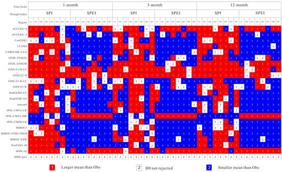
Figure 3.
Result of Dunnett multiple comparisons between climate models simulation data and observed data in the historical period.
In the MME-all, only SPI1 of SR6 and SPI2 of SR2 do not reject the H0. This was due to MME-all being affected by most of the models which rejected the H0 for SPI, SPEI, and some SRs. It means that MME-all cannot be reproduced with the drought frequency of observation. MME-part shows good consistency with observed data. Because MME-part was composed of models that have no rejection H0, it could be reproduced with the drought frequency of observed data. In this study, Bayesian model averaging (BMA) was used to reproduce the future drought conditions. Compared with simple model averaging, BMA is considered to have the best potential to reproduce the future drought conditions in dryland Asia [36].
3.3. Future Drought Frequency
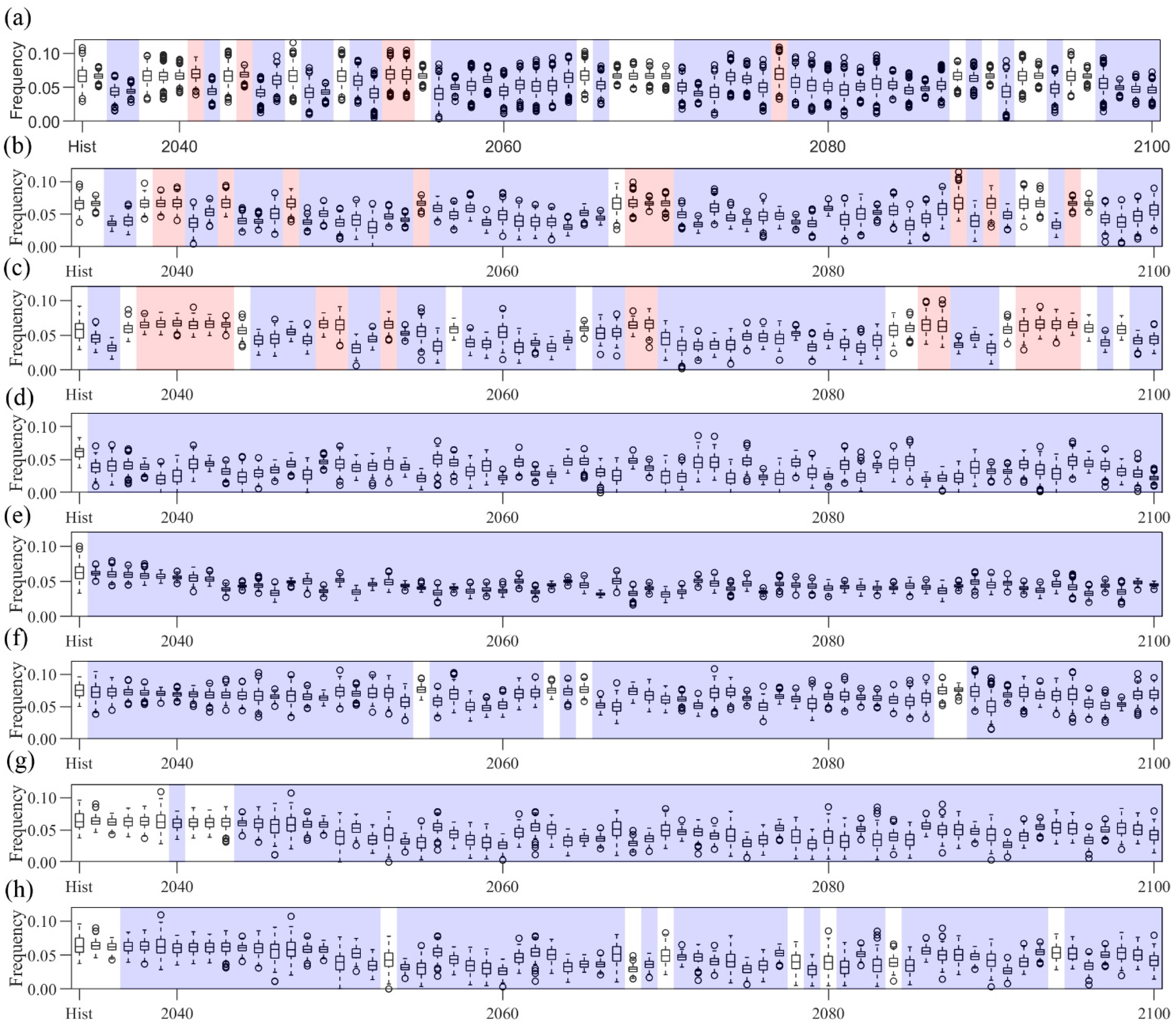
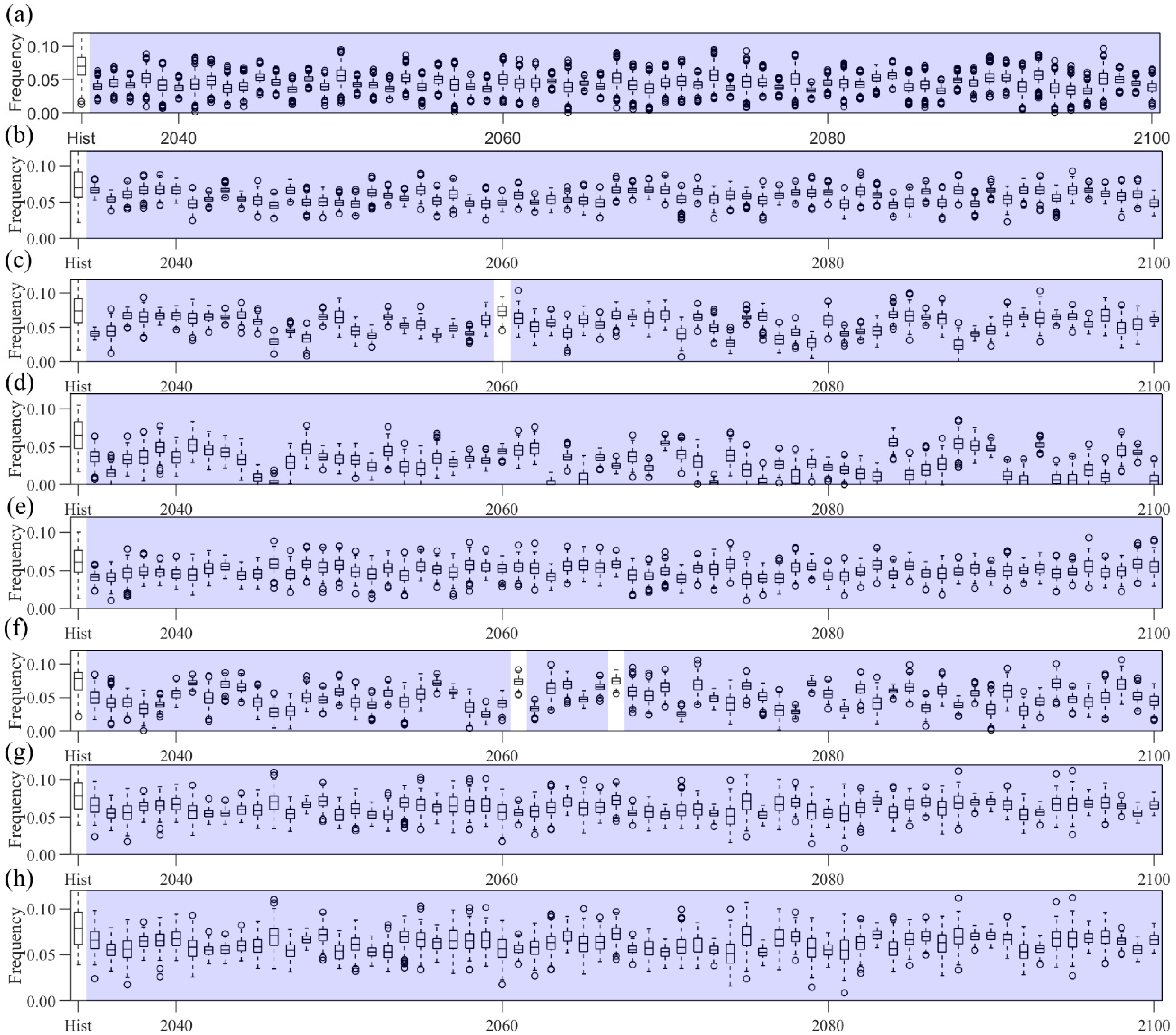
The drought frequency was calculated for SPI and SPEI in each SR under RCP 4.5 scenarios from 2006 to 2100. Dunnett multiple comparisons were used to test whether future drought frequencies are consistent with the historical periods (Figure 4, Figure 5, Figure 6, Figure 7, Figure 8 and Figure 9). The null hypothesis H0 is that there is no difference in the frequency of severe or extreme drought between future and historical periods, and the significance level is 0.05. The frequency of severe or extreme drought in the future is larger than or smaller than the historical period, which indicates that the severe or extreme drought frequency will increase or decrease in the future.
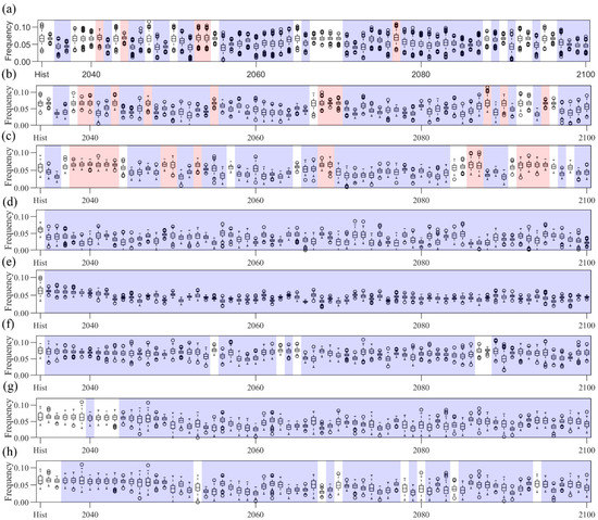
Figure 4.
Frequency of drought based on SPI1 in entire CA (a), (b) SR1, (c) SR2, (d) SR3, (e) SR4, (f) SR5, (g) SR6, and (h) SR7. Hist represents the drought frequency for historical period. Boxplots display the values ranges of grids data belonging to corresponding drought subregions, and the outliers are replaced by circles.
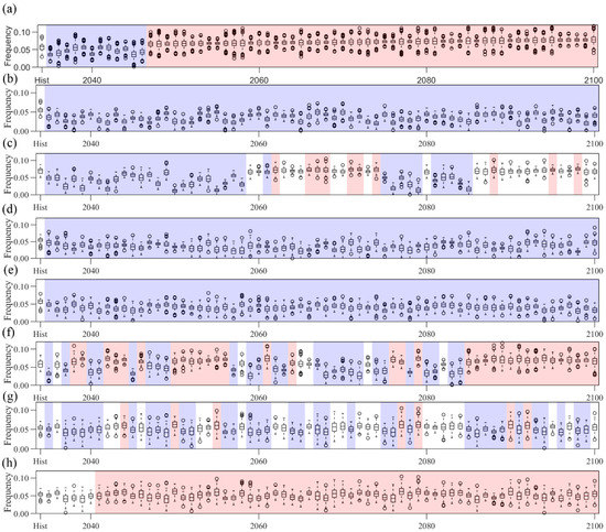
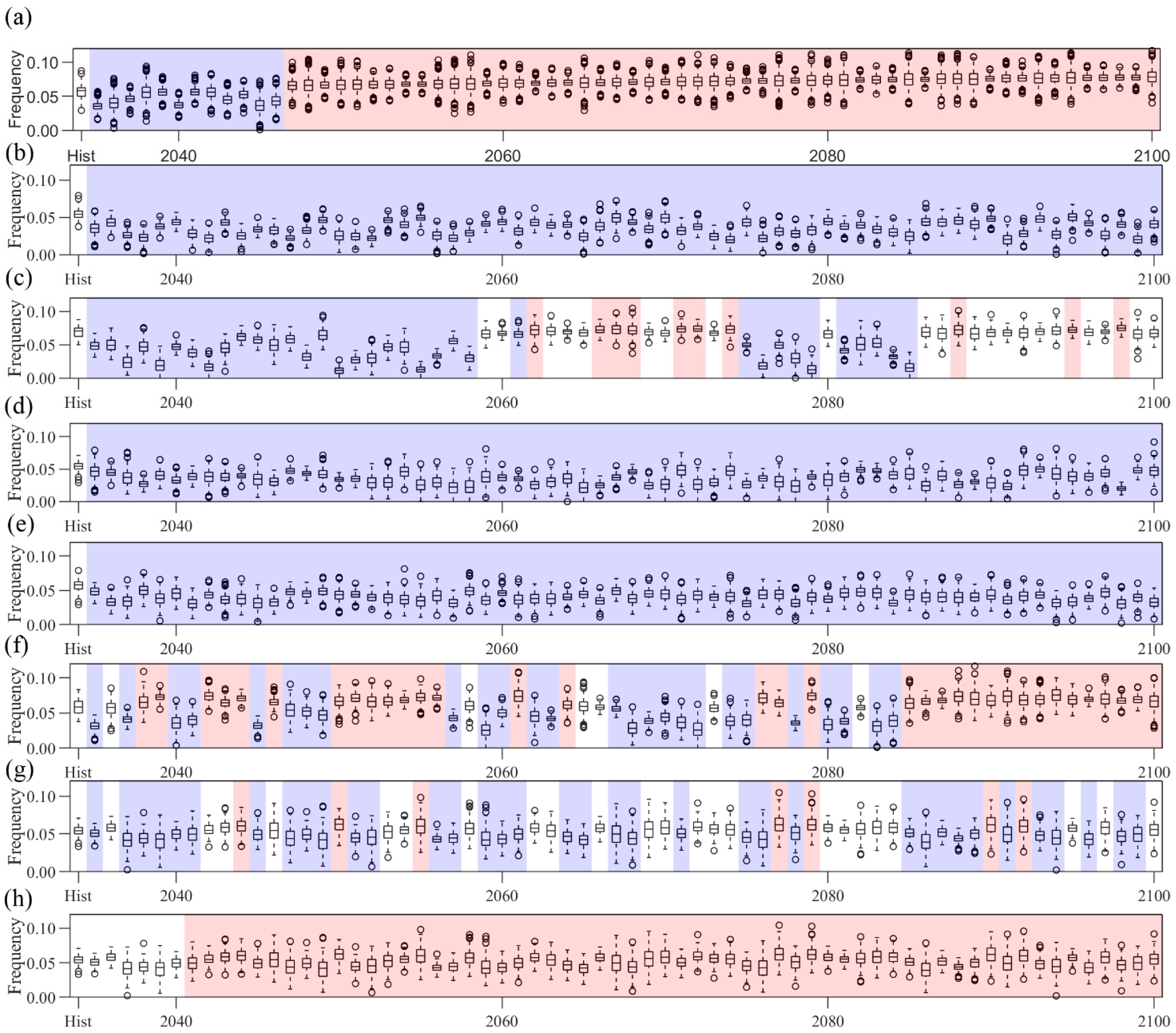
Figure 5.
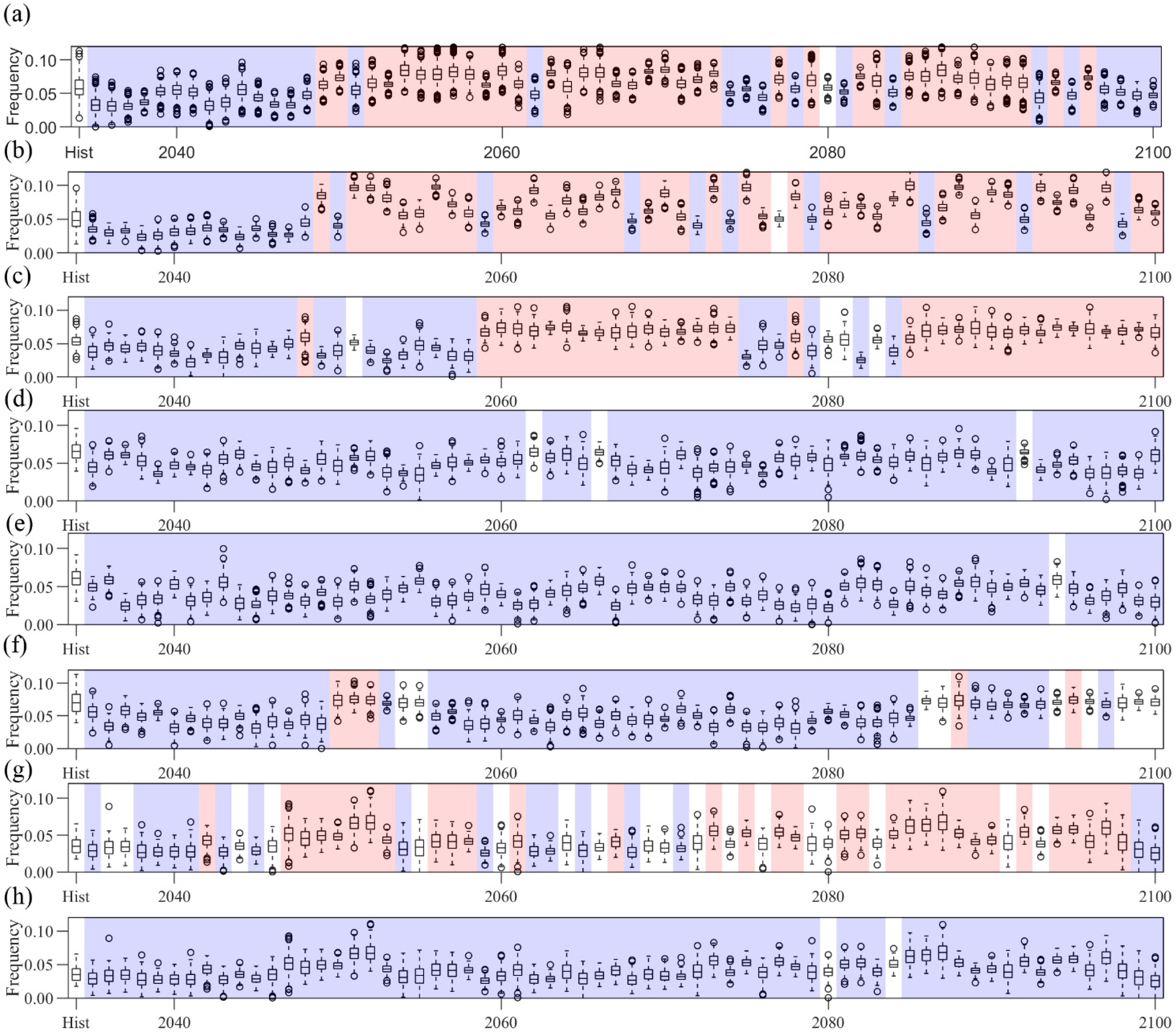
Frequency of drought based on SPEI1 in entire CA (a), (b) SR1, (c) SR2, (d) SR3, (e) SR4, (f) SR5, (g) SR6, and (h) SR7. Hist represents the drought frequency for historical period. Boxplots display the values ranges of grids data belonging to corresponding drought subregions, and the outliers are replaced by circles.
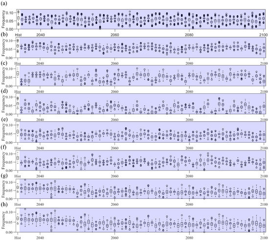
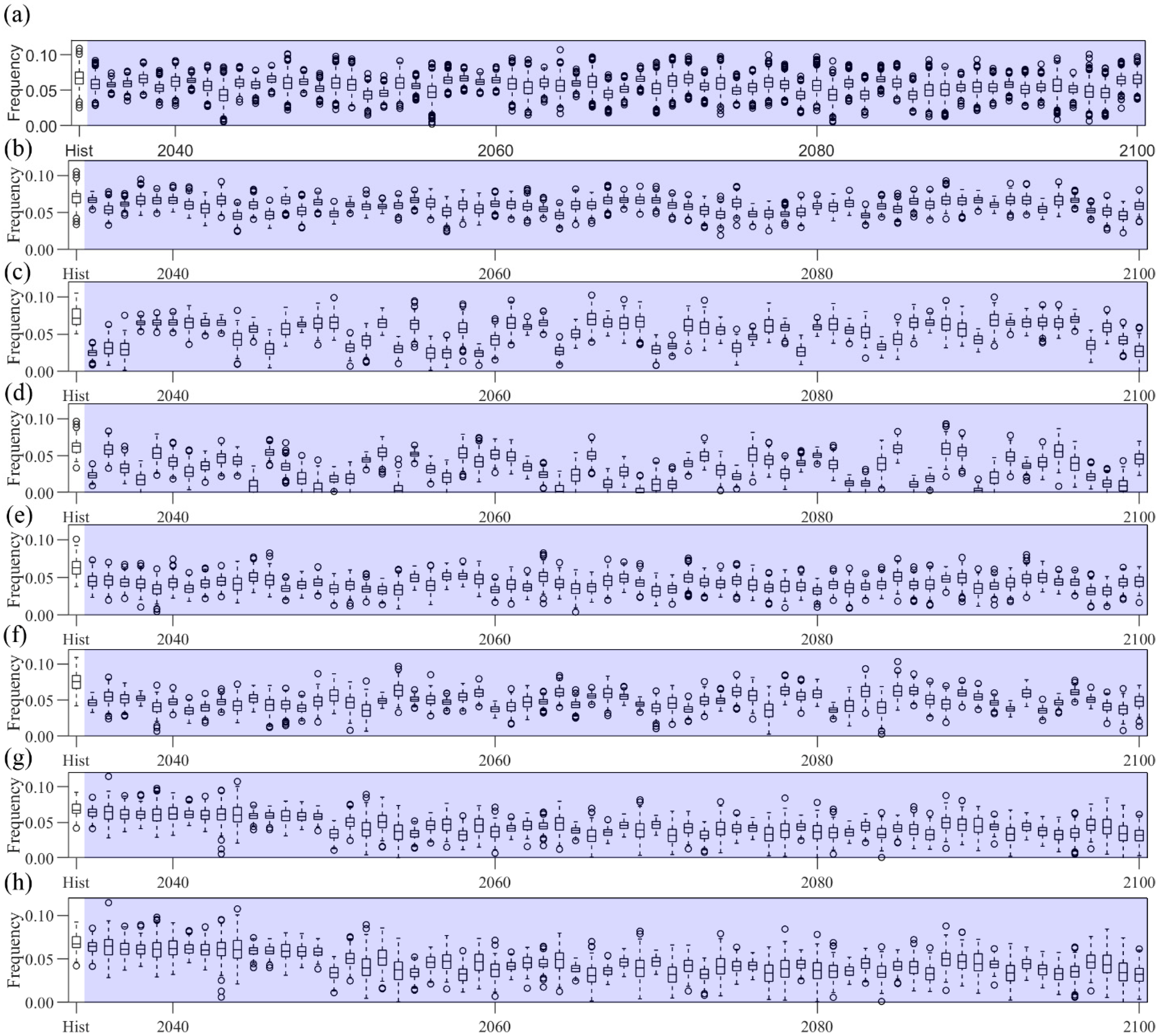
Figure 6.
Frequency of drought based on SPI3 in entire CA (a), (b) SR1, (c) SR2, (d) SR3, (e) SR4, (f) SR5, (g) SR6, and (h) SR7. Hist represents the drought frequency for historical period. Boxplots display the values ranges of grids data belonging to corresponding drought subregions, and the outliers are replaced by circles.
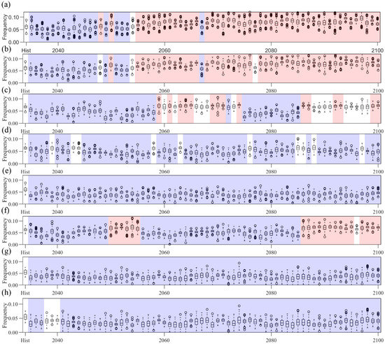
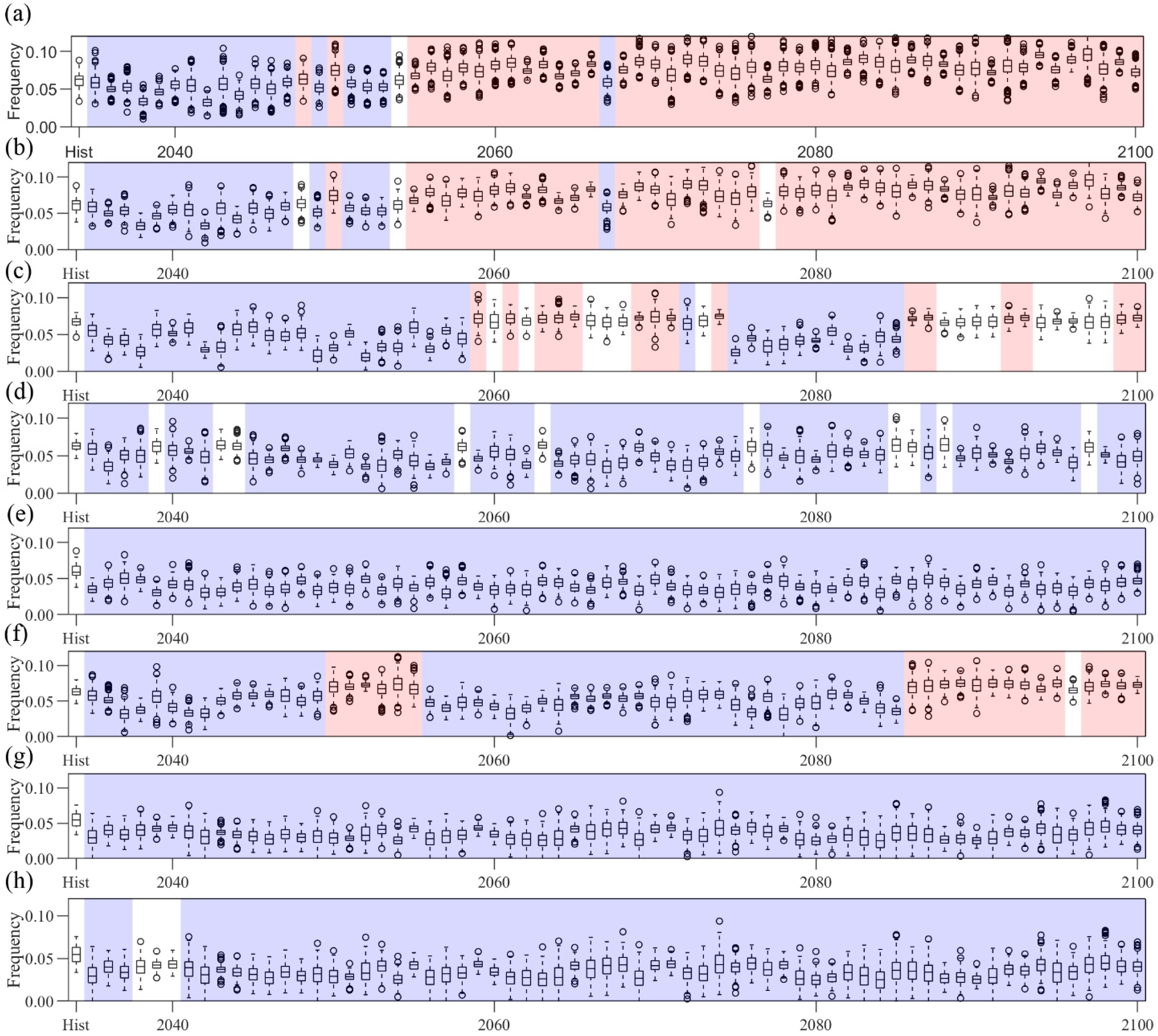
Figure 7.
Frequency of drought based on SPEI3 in entire CA (a), (b) SR1, (c) SR2, (d) SR3, (e) SR4, (f) SR5, (g) SR6, and (h) SR7. Hist represents the drought frequency for historical period. Boxplots display the values ranges of grids data belonging to corresponding drought subregions, and the outliers are replaced by circles.
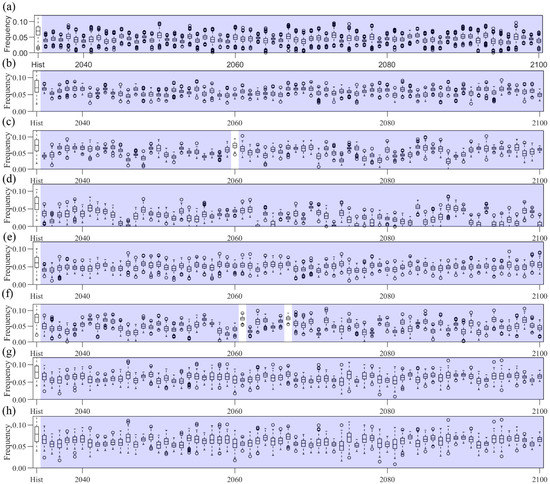
Figure 8.
Frequency of drought based on SPI12 in entire CA (a), (b) SR1, (c) SR2, (d) SR3, (e) SR4, (f) SR5, (g) SR6, and (h) SR7. Hist represents the drought frequency for historical period. Boxplots display the values ranges of grids data belonging to corresponding drought subregions, and the outliers are replaced by circles.
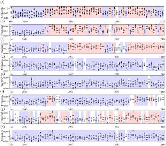
Figure 9.
Frequency of drought based on SPEI12 in entire CA (a), (b) SR1, (c) SR2, (d) SR3, (e) SR4, (f) SR5, (g) SR6, and (h) SR7. Hist represents the drought frequency for historical period. Boxplots display the values ranges of grids data belonging to corresponding drought subregions, and the outliers are replaced by circles.
The analysis of future drought frequency was performed using MME-part for SPI and SPEI throughout the CA and each SR. The boxplot shows each 30-year period severe or extreme drought frequency distribution for all grids located in the corresponding SR. As we can see from Figure 4a, in the future, the frequency of severe or extreme drought in most years is between 0 and 0.05, which is significantly smaller than that in the historical period. It means that the future drought frequency will decrease based on SPI1 in CA. The seven drought subregions also show the decreased drought frequency based on SPI1 (Figure 4b–h). The drought frequency in SR2 (Figure 4c) fluctuated between 0 and 0.1. While the other SRs are below 0.05, especially in SR6 (Figure 4g) and SR7 (Figure 4h), the severe or extreme drought frequency is lower than in the historical period.
For SPEI1, the severe or extreme drought frequency is between 0 and 0.10 in CA (Figure 5a). Before the period ending year (PEY) 2047, the drought frequency is smaller than the historical period, and after PEY 2047, the frequency shows an increasing trend. In 2047, the drought frequency is larger than the historical period. The H0 was rejected for all future periods for SR1 (Figure 5b), SR3 (Figure 5d), SR4 (Figure 5e), and SR6 (Figure 5g) and show smaller means than the historical period. For SR2 (Figure 5c), SR5 (Figure 5f), and SR7 (Figure 5h), drought frequency shows an increasing trend in the future period.
No significant drought frequency change was detected based on SPI3 in the CA (Figure 6a). The drought frequency shows a decrease, and the value is below 0.05 in the future period. Results in the other SRs show the same downward trend.
The future drought frequency based on SPEI3 is a decrease in the early future periods in CA (Figure 7a), and an increase in the PEY 2055. For SR1 (Figure 7b), the values of drought frequency between 2055 and 2100 are greater than or equal to the historical period, and the values will increase continuously in the PEY 2055. The drought frequencies of SR2 (Figure 7c) are larger than or equal to the historical period among PEY2059-PEY2074 and PEY2086-PEY2100. In early and middle future periods, SR5’s drought frequencies (Figure 7f) show a downward trend, which increase in PEY2050-PEY2055 and PEY2086-PEY2100. The results in SR3 (Figure 7c), SR4 (Figure 7e), SR6 (Figure 7g), and SR7 (Figure 7h) are the same, both smaller than the historical period.
For SPI12 (Figure 8), the drought frequencies were projected to decease for most years in the future periods relative to the historical period over CA (Figure 8a). The drought frequencies in SR1 (Figure 8b), SR2 (Figure 8c), SR3 (Figure 8d), SR4 (Figure 8e), SR5 (Figure 8f), SR6 (Figure 8g), and SR7 (Figure 8h) are smaller than the historical period.
As shown in Figure 9a, we can see that the future drought frequencies based on SPEI12 were declining relative to the historical period in the early future period in CA. From the PEY2049 to PEY2100, the drought frequencies are larger than the historical period. In SR1 (Figure 9b), SR2 (Figure 9b), and SR6 (Figure 9g), the drought frequencies in middle and later future periods are larger than those in the historical periods, and the drought frequencies in the early future periods are smaller than the historical periods. The drought frequencies in SR3 (Figure 9d), SR4 (Figure 9e), and SR7 (Figure 9h) are smaller than those in the historical period.
3.4. Future Drought Duration
As with the frequency of drought, the duration of drought is an important variable to describe drought condition. Drought duration refers to the start and end time of an event during a drought. The drought event means that the drought indices (SPI and SPEI) are less than −1.5. In this study, we employed the average duration of drought for each drought index and SR. The null hypothesis is used for the case when there is no difference between the future period and historical period. If the average value is larger or smaller than the historical observation value, it indicates that the average drought duration will increase or decrease in the future. We analyzed the average drought duration for both SPI1 and SPEI1.
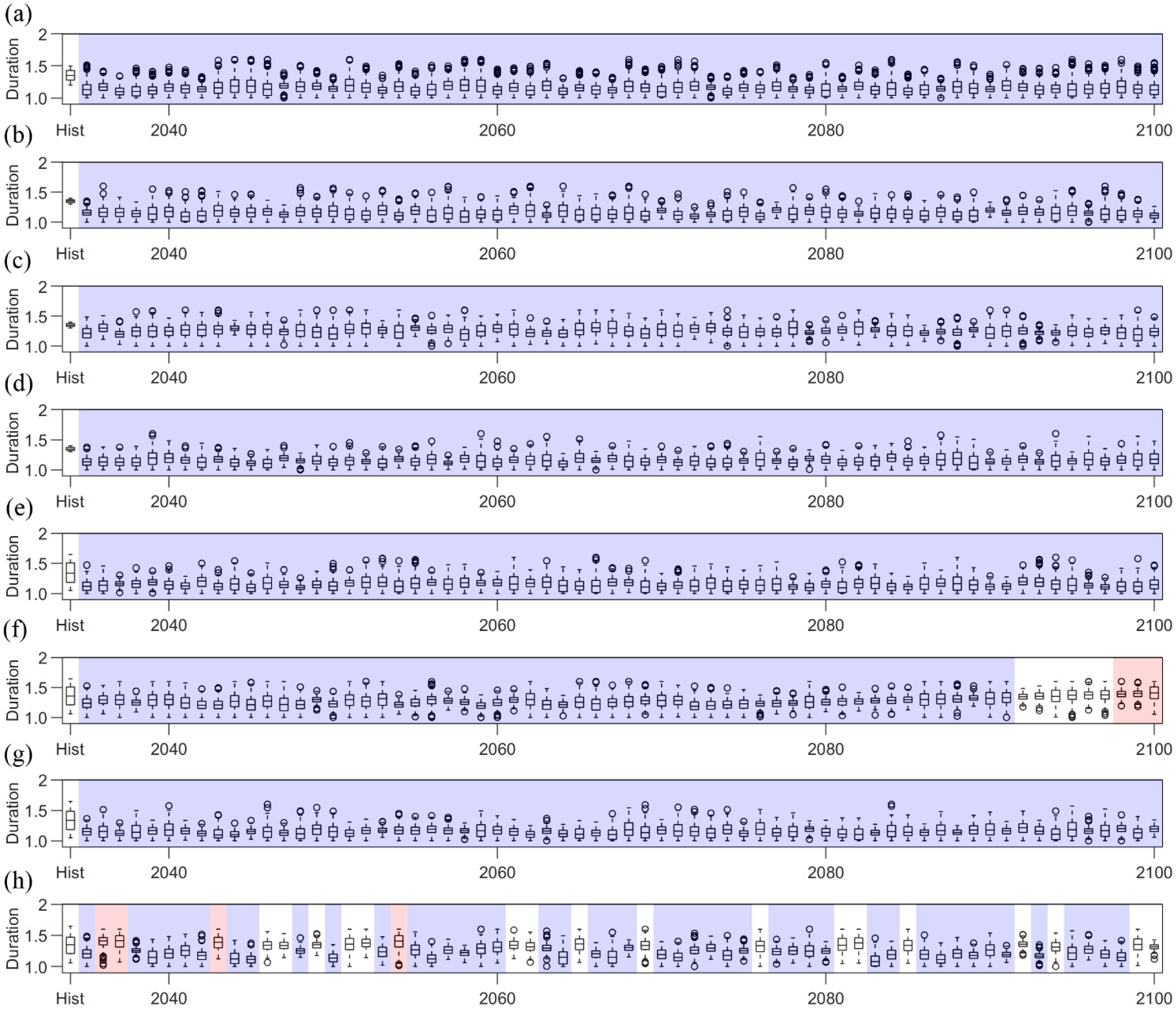
The drought duration based on SPI1 in the future period is smaller than the historical period in CA (Figure 10a). The same can be seen for the SR1 (Figure 10b), SR2 (Figure 10c), SR3 (Figure 10d), SR4 (Figure 10e), SR5 (Figure 10f), SR6 (Figure 10g), and SR7 (Figure 10h); the drought duration of the future period is smaller than the historical period.
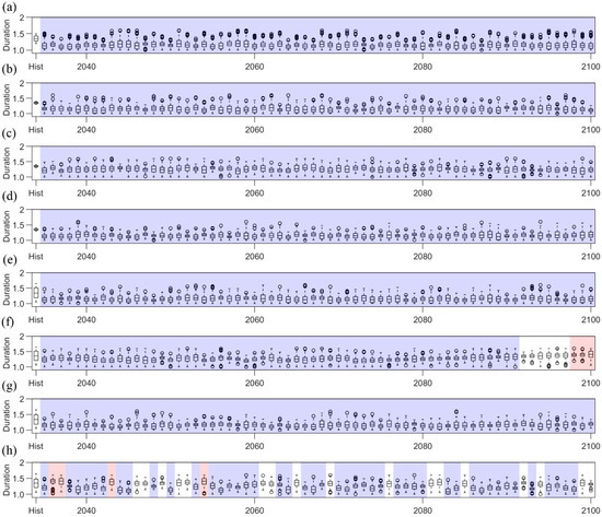
Figure 10.
Duration of drought based on SPI1 in entire CA (a), (b) SR1, (c) SR2, (d) SR3, (e) SR4, (f) SR5, (g) SR6, and (h) SR7. Hist represents the drought frequency for historical period. Boxplots display the values ranges of grids data belonging to corresponding drought subregions, and the outliers are replaced by circles.
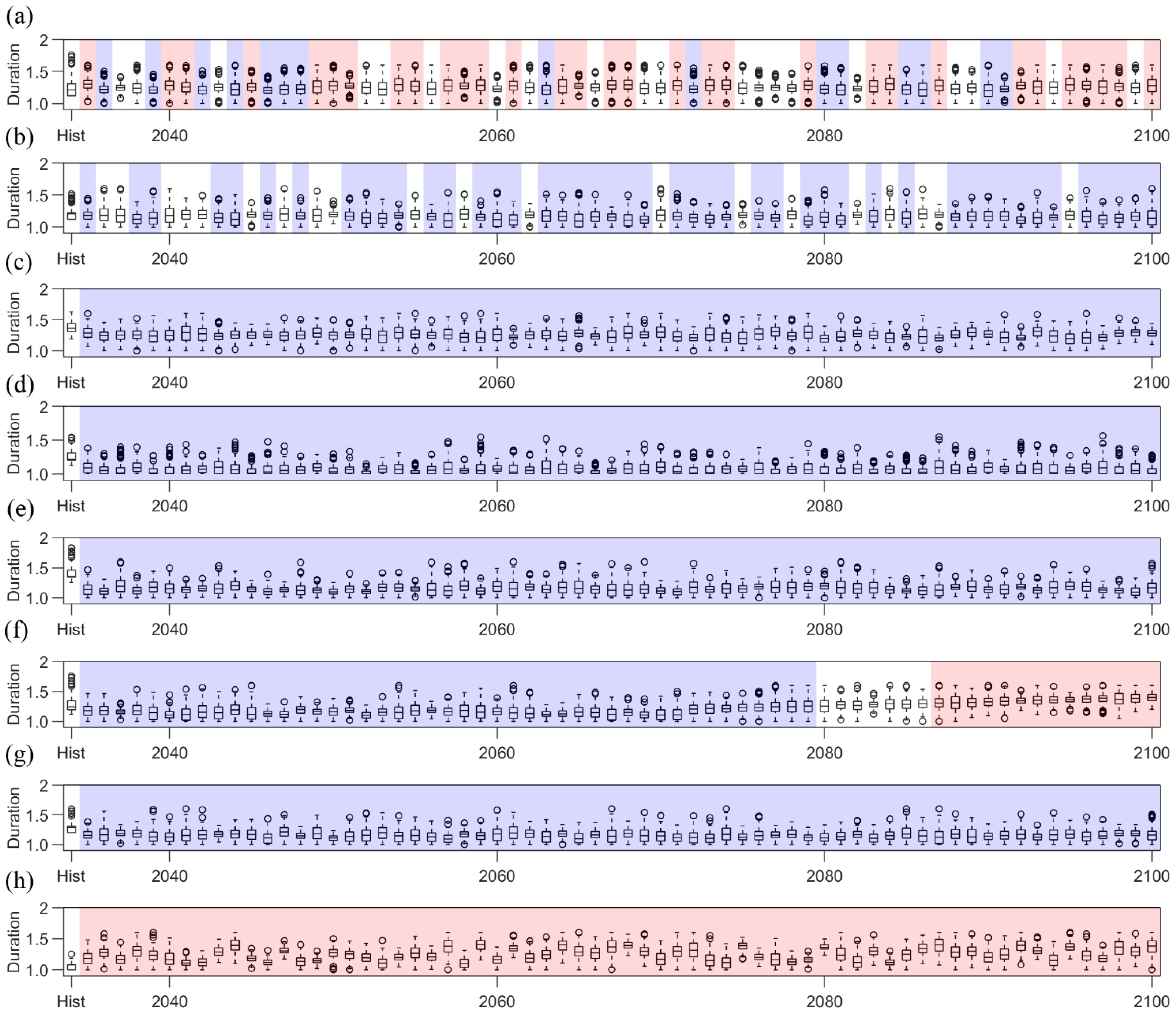
For SPEI1, the average drought duration of most future periods in CA (Figure 11a) are longer than historical period. In the SR1 (Figure 11b), SR2 (Figure 11c), SR3 (Figure 11d), SR4 (Figure 11e), and SR6 (Figure 11g), decreases in drought duration were projected in the future period. The drought duration was projected to increase in the later future period for SR5 (Figure 11f). Only the drought duration showed an increase in all future periods for SR7 (Figure 11h).
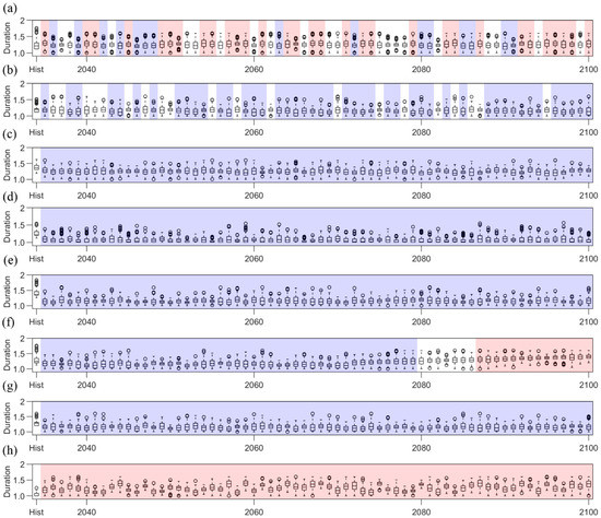
Figure 11.
Duration of drought based on SPEI1 in entire CA (a), (b) SR1, (c) SR2, (d) SR3, (e) SR4, (f) SR5, (g) SR6, and (h) SR7. Hist represents the drought frequency for historical period. Boxplots display the values ranges of grids data belonging to corresponding drought subregions, and the outliers are replaced by circles.
4. Conclusions and Discussion
The characteristics of future drought changes in Central Asia were predicted by using 21 bias-correction climate models under RCP4.5. Dunnett multiple comparisons were applied to detect if there is a difference between the future periods and historical periods. SPI and SPEI of 1, 3, and 12 months were selected as drought indicators. Drought frequency and drought duration are two important indicators to describe drought. We calculated the frequency of droughts for each drought index, drought conditions, historical periods, and future periods on timescales, with the aim of selecting suitable climate models such as MME-part to reproduce the drought characteristic of the historical periods. The drought frequency and duration of MME-part were calculated for each drought subregion and all drought indexes to examine the future drought changes in CA.
The drought frequencies in the future periods based on SPI1 and SPI3 are similar. The drought frequencies are smaller than the historical period and are below 0.05. In the entire CA and other SRs, decreases in drought frequencies are projected based on SPI1 and SPI3 in all future periods, but for the future drought frequency of SPI12, the average drought frequency in Central Asia shows a consistent increase with SR6 in the later future periods. In other SRs, the drought frequencies based on SPI12 are smaller than those of the historical periods and show a decrease in all future periods. The characteristics of drought frequency based on SPEI are different from SPI. The average drought frequencies of CA based on SPEI1, SPEI3, and SPEI12 show a decrease in the early future periods as well as an increase in the middle and later future periods. Different drought indices have different predictions about the frequency of future droughts. It is found that the projected results of future drought frequency are different based on SPI and SPEI. For instance, both SPI12 and SPEI12 can predict the increase and decrease in future periods. However, SPEI12 predicts an increase in most future periods, and SPI12 mostly predicts a decrease in average drought frequency in CA. These discrepancies between SPI and SPEI are caused by the fact that SPI ignores temperature, evaporation, and other climate variables, while SPEI applies evapotranspiration and considers the water and heat balance. In general, SPI is selected as the drought indicator, and the frequency of future drought in Central Asia shows a deceasing trend, but for SPEI, the drought frequency shows an increasing trend. The prediction results of different drought indices for future drought frequency in Central Asia are completely different, which indicates the importance of selecting the appropriate drought index.
As for the drought duration, the SPI and SPEI also show contrasting results in predicting the drought duration. For the average drought duration of CA, the future drought duration based on SPI is not significantly different from the historical drought duration, whereas the future drought duration based on SPEI decreases in the early future periods and increases in the middle and later future periods.
Author Contributions
Conceptualization, Z.T.; methodology, K.L.; resources, Y.Y.; writing—original draft preparation, Z.T.; writing—review and editing, M.Y. All authors have read and agreed to the published version of the manuscript.
Funding
This research was funded by the Natural Science Foundation of Shaanxi province, China (Grant No. 2021JQ-771) and Research Project of Shaanxi Provincial Department of Education (Grant No. 21JK0305 and SGH20Q231). The APC was funded by Natural Science Foundation of Shaanxi province, China (Grant No. 2021JQ-771).
Institutional Review Board Statement
Not applicable.
Informed Consent Statement
Not applicable.
Data Availability Statement
Access the data can contact the E-mail: tazhijie@xisu.edu.cn.
Acknowledgments
We acknowledge the World Climate Research Programme (WCRP) Working Group on Coupled Modelling (WGCM) for providing access to the CMIP5 climate model outputs was used in this study. The authors are very grateful to the anonymous reviewers and editors for their critical review and comments which helped to improve and clarify the paper.
Conflicts of Interest
The authors declare that they have no conflict of interest.
References
- Shiru, M.S.; Chung, E.S.; Shahid, S.; Alias, N. GCM selection and temperature projection of Nigeria under different RCPs of the CMIP5 GCMS. Theor. Appl. Climatol. 2020, 141, 1611–1627. [Google Scholar] [CrossRef]
- Gupta, A.; Rico-Medina, A.; Cao-Delgado, A.I. The physiology of plant responses to drought. Science 2020, 368, 266–269. [Google Scholar] [CrossRef] [PubMed]
- Zhang, R.; Liang, T.; Guo, J.; Xie, H.; Feng, Q.; Aimaiti, Y. Grassland dynamics in response to climate change and human activities in Xinjiang from 2000 to 2014. Entific Rep. 2018, 8, 2888. [Google Scholar] [CrossRef] [PubMed]
- Seneviratne, S. Changes in climate extremes and their impacts on the natural physical environment: An overview of the IPCC SREX report. In Managing the Risks of Extreme Events and Disasters to Advance Climate Change Adaptation; Cambridge University Press: Cambridge, UK, 2012. [Google Scholar]
- Burke, E.J.; Brown, S.J. Evaluating Uncertainties in the Projection of Future Drought. J. Hydrometeorol. 2008, 9, 292–299. [Google Scholar] [CrossRef]
- Botterill, L.C.; Hayes, M.J. Drought triggers and declarations: Science and policy considerations for drought risk management. Nat. Hazards 2012, 64, 139–151. [Google Scholar] [CrossRef] [Green Version]
- Svoboda, M.; Fuchs, B.A.; Poulsen, C.C.; Nothwehr, J.R. The drought risk atlas: Enhancing decision support for drought risk management in the United States. J. Hydrol. 2015, 526, 274–286. [Google Scholar] [CrossRef] [Green Version]
- Zhai, J.; Mondal, S.K.; Fischer, T.; Wang, Y.; Su, B.; Huang, J.; Tao, H.; Wang, G.; Ullah, W.; Uddin, M.J. Future drought characteristics through a multi-model ensemble from CMIP6 over South Asia. Atmos. Res. 2020, 246, 105111. [Google Scholar] [CrossRef]
- Lin, W.; Wen, C. A CMIP5 multimodel projection of future temperature, precipitation, and climatological drought in China. Int. J. Climatol. 2014, 34, 2059–2078. [Google Scholar]
- Swain, S.; Hayhoe, K. CMIP5 projected changes in spring and summer drought and wet conditions over North America. Clim. Dyn. 2015, 44, 2737–2750. [Google Scholar] [CrossRef]
- Venkataraman, K.; Tummuri, S.; Medina, A.; Perry, J. 21st century drought outlook for major climate divisions of Texas based on CMIP5 multimodel ensemble: Implications for water resource management. J. Hydrol. 2016, 534, 300–316. [Google Scholar] [CrossRef] [Green Version]
- Khan, J.U.; Islam, A.; Das, M.K.; Mohammed, K.; Islam, G. Future changes in meteorological drought characteristics over Bangladesh projected by the CMIP5 multi-model ensemble. Clim. Chang. 2020, 162, 667–685. [Google Scholar] [CrossRef]
- Erol, A.; Randhir, T.O. Climatic change impacts on the ecohydrology of Mediterranean watersheds. Clim. Chang. 2012, 114, 319–341. [Google Scholar] [CrossRef]
- Almazroui, M.; Islam, M.N. Coupled Model Inter-comparison Project Database to Calculate Drought Indices for Saudi Arabia: A Preliminary Assessment. Earth Syst. Environ. 2019, 3, 419–428. [Google Scholar] [CrossRef]
- Dai, A. Increasing drought under global warming in observations and models. Nat. Clim. Chang. 2013, 3, 52–58. [Google Scholar] [CrossRef]
- Kai, X.; Cwa, B.; Czc, D.; Bxha, B. Uncertainty assessment of drought characteristics projections in humid subtropical basins in China based on multiple CMIP5 models and different index definitions—ScienceDirect. J. Hydrol. 2021, 600, 126502. [Google Scholar]
- Gm, A.; Vm, B.; Dn, C.; St, D.; Rao, S. Trends and variability of droughts over the Indian monsoon region. Weather Clim. Extrem. 2016, 12, 43–68. [Google Scholar]
- Ruosteenoja, K.; Markkanen, T.; Venlinen, A.; Risnen, P.; Peltola, H. Seasonal soil moisture and drought occurrence in Europe in CMIP5 projections for the 21st century. Clim. Dyn. 2018, 50, 1177–1192. [Google Scholar] [CrossRef] [Green Version]
- Wu, C.; Yeh, J.F.; Chen, Y.Y.; Lv, W.; Huang, G. Copula-based risk evaluation of global meteorological drought in the 21st century based on CMIP5 multi-model ensemble projections. J. Hydrol. 2021, 126265. [Google Scholar] [CrossRef]
- Vicente-Serrano, S.M.; Beguería, S.; López-Moreno, J. A Multiscalar Drought Index Sensitive to Global Warming: The Standardized Precipitation Evapotranspiration Index. J. Clim. 2010, 23, 1696–1718. [Google Scholar] [CrossRef] [Green Version]
- Wells, N.; Goddard, S.; Hayes, M.J. A Self-Calibrating Palmer Drought Severity Index. J. Clim. 2004, 17, 2335–2351. [Google Scholar] [CrossRef]
- Sheffield, J.; Andreadis, K.M.; Wood, E.F.; Lettenmaier, D.P. Global and Continental Drought in the Second Half of the Twentieth Century: Severity–Area–Duration Analysis and Temporal Variability of Large-Scale Events. J. Clim. 2009, 22, 1962–1981. [Google Scholar] [CrossRef]
- Chen, X.; Bai, J.; Li, X.; Luo, G.; Li, J.; Li, B.L. Changes in land use/land cover and ecosystem services in Central Asia during 1990–2009. Curr. Opin. Environ. Sustain. 2013, 5, 116–127. [Google Scholar] [CrossRef]
- Moss, R.H.; Edmonds, J.A.; Hibbard, K.A.; Manning, M.R.; Rose, S.K.; Vuuren, D.P.V.; Carter, T.R.; Emori, S.; Kainuma, M.; Kram, T. The next generation of scenarios for climate change research and assessment. Nature 2010, 463, 747–756. [Google Scholar] [CrossRef] [PubMed]
- Gudmundsson, L.; Bremnes, J.B.; Haugen, J.E.; Engenskaugen, T. Technical Note: Downscaling RCM precipitation to the station scale using statistical transformations—A comparison of methods. Hydrol. Earth Syst. Sci. Discuss. 2012, 9, 6185–6201. [Google Scholar] [CrossRef] [Green Version]
- Rhee, J.; Cho, J. Future Changes in Drought Characteristics: Regional Analysis for South Korea under CMIP5 Projections. J. Hydrometeorol. 2015, 17, 151016095329004. [Google Scholar] [CrossRef]
- Sunyer, M.A.; Madsen, H.; Ang, P.H. A comparison of different regional climate models and statistical downscaling methods for extreme rainfall estimation under climate change. Atmos. Res. 2012, 103, 119–128. [Google Scholar] [CrossRef]
- Moetasim, A.; Bowling, L.C.; Keith, C.; Pal, J.S.; Diffenbaugh, N.S. Influence of climate model biases and daily-scale temperature and precipitation events on hydrological impacts assessment: A case study of the United States. J. Geophys. Res. Atmos. 2010, 45, 1099–1116. [Google Scholar]
- Themeßl, M.J.; Gobiet, A.; Leuprecht, A. Empirical-statistical downscaling and error correction of daily precipitation from regional climate models. Int. J. Climatol. 2011, 31, 1530–1544. [Google Scholar] [CrossRef]
- Yang, P.; Xia, J.; Zhang, Y.; Zhan, C.; Qiao, Y. Comprehensive assessment of drought risk in the arid region of Northwest China based on the global palmer drought severity index gridded data. Sci. Total Environ. 2018, 627, 951–962. [Google Scholar] [CrossRef]
- Taylor, I.H.; Burke, E.; Mccoll, L.; Falloon, P.D.; Harris, G.R.; Mcneall, D. The impact of climate mitigation on projections of future drought. Hydrol. Earth Syst. Sci. 2013, 17, 2339–2358. [Google Scholar] [CrossRef] [Green Version]
- Hayes, M.; Svoboda, M.; Wall, N.; Widhalm, M. The Lincoln Declaration on Drought Indices: Universal Meteorological Drought Index Recommended. Bull. Am. Meteorol. Soc. 2011, 92, 485–488. [Google Scholar] [CrossRef] [Green Version]
- Vicenteserrano, S.M.; Lópezmoreno, J.I. Hydrological response to different time scales of climatological drought: An evaluation of the Standardized Precipitation Index in a mountainous Mediterranean basin. Hydrol. Earth Syst. Sci. 2005, 9, 523–533. [Google Scholar] [CrossRef] [Green Version]
- Guo, H.; He, S.; Li, M.; Bao, A.; Chen, T.; Zheng, G.; Maeyer, P.D. Future changes of drought characteristics in CMIP6 SSP scenarios over Central Asia. Int. J. Climatol. 2021. [Google Scholar] [CrossRef]
- Dunnett, C.W. A Multiple Comparison Procedure for Comparing Several Treatments with a Control. Publ. Am. Stat. Assoc. 1955, 50, 1096–1121. [Google Scholar] [CrossRef]
- Miao, L.; Ye, P.; He, B.; Chen, L.; Cui, X. Future Climate Impact on the Desertification in the Dry Land Asia Using AVHRR GIMMS NDVI3g Data. Remote Sens. 2015, 7, 3863–3877. [Google Scholar] [CrossRef] [Green Version]

Publisher’s Note: MDPI stays neutral with regard to jurisdictional claims in published maps and institutional affiliations. |
© 2022 by the authors. Licensee MDPI, Basel, Switzerland. This article is an open access article distributed under the terms and conditions of the Creative Commons Attribution (CC BY) license (https://creativecommons.org/licenses/by/4.0/).