Does the El Niño-Southern Oscillation Affect the Combined Impact of the Atlantic Multidecadal Oscillation and Pacific Decadal Oscillation on the Precipitation and Surface Air Temperature Variability over South America?

Abstract

Previous studies have shown that the Atlantic Multidecadal Oscillation (AMO) and Pacific Decadal Oscillation (PDO) have combined effects on the precipitation (PRP) variability over South America. The combined impacts have been assessed considering four mean states as the averages of the variable anomalies during sub-periods overlapping time intervals of the PDO and AMO phases. Since these sub-periods include years under El Niño-Southern Oscillation (ENSO) extremes, the extent to which these years’ occurrence affects the averaged anomaly patterns during different mean states is investigated. The analyses are done for the PRP and surface air temperature (SAT) during the austral winter (June to August) and summer (December to February) of the 1901–2014 period using a composite technique. The nonlinear ENSO response in each mean state for a variable corresponds to the sum of the anomaly composites of the El Niño and La Niña events. In each mean state, the nonlinear PRP and SAT anomalies are not negligible and show similar patterns of the corresponding mean state, with larger magnitudes. For both seasons and all mean states, these similarities are more pronounced for SAT than for PRP. Thus, the ENSO variability affects the mean state’s PRP and SAT anomaly patterns in different ways. As far as we know, analyses of the nonlinear ENSO response of the South American climate during distinct mean states were not performed before. Our results also indicate that the ENSO variability should be considered in the studies of the low-frequency modes and their effects on the mean state over South America. The results presented could be relevant for climate monitoring and modeling studies.

1. Introduction

South America presents diverse regional climates characterized by distinct seasonal precipitation (PRP) and surface air temperature (SAT) distributions. The interannual climate variability in this region is primarily modulated by the El Niño-Southern Oscillation (ENSO) through large-scale atmospheric teleconnections, which modulate PRP and SAT in distinct ways depending on the season and area. The ENSO-related PRP anomaly patterns in this continent have been extensively documented and feature a dipole for annual PRP with one node in its northern-northeastern sector (northern equatorial Brazil, French Guiana, Surinam, and Venezuela) and the other in its southeastern sector (southeastern Brazil, Uruguay, and northeastern Argentina) [1,2,3,4,5,6,7]. This dipole is anomalously dry-wet during El Niño (EN) events, and an opposite sign dipole during La Niña (LN) events [8]. The ENSO teleconnections in the equatorial sector are driven by variations in the Walker cell [1,2,3,9,10], and in the subtropical sector, by the Rossby-wave trains induced by the anomalous tropical heat source (sink) [11,12]. Most analyses of the ENSO effects on the climate of South America focused on the PRP due to the weak ENSO impacts on SAT in this continent [13]. However, a few studies registered EN-related anomalous warming in its subtropical and southeastern sectors during austral winter, most of its tropical area during summer and autumn, and along the northern coast and western tropical sector during spring [9,10,13,14,15,16,17,18,19].

Nevertheless, several studies have shown that the ENSO extremes are modulated by low-frequency modes such as the Pacific Decadal Oscillation (PDO) [20] and the Atlantic Multidecadal Oscillation (AMO). Chen et al. [21] showed that the AMO modulates the influence of the winter North Pacific Oscillation on the following winter ENSO, such that this influence is strong during the cold AMO and weak during the warm AMO. On the other hand, Kim et al. [22] found that the sensitivity of the EN frequency to the AMO is strong during the cold PDO and weak during the warm PDO.

Notwithstanding, the PDO and AMO varying in slightly different multidecadal time scales (50–70-years and 60–80-years, respectively) might be connected through an atmospheric bridge between the tropical Pacific and Atlantic Oceans [23,24,25,26]. In this vein, the abnormal acceleration of the Pacific trade winds, Walker cell intensification, and the eastern Pacific cooling since the early 1990s were associated with the Atlantic warming in the 30° S–60° N sector [23]. Kucharski et al. [25] provided modeling and diagnostic evidence that the warm AMO induces the eastern Pacific cooling and the western Pacific/Indian Oceans warming, and the cold AMO produces opposite conditions in these Oceans. These results suggest linkages between the AMO and PDO. In this context, several studies have shown that the AMO and PDO have combined effects in the ENSO teleconnections in several regions of the globe, such as the southeastern United States [27] and South America [28,29,30]. Concerning the South American climate, the AMO and PDO combined effects at a multidecadal time scale [31] were investigated, and in the Choco and Caribbean, low-level jets with regional implications for the Colombian climate [30] were also examined.

In addition, the time intervals overlapping the AMO and PDO phases represent different anomaly mean states of the sea surface temperature (SST) in the Pacific and Atlantic Oceans. Using ‘W’ and ‘C’ to refer to warm and cold phases, and ‘A’ and ‘P’ to refer to AMO and PDO, respectively, the acronymous of the four possible mean states are CACP, CAWP, WACP, and WAWP. Except for the WAWP, Kayano et al. [29] analyzed the seasonal anomaly patterns of SST and PRP over South America, as well as the vertical velocity in pressure levels for these mean states during the 1901–2011 period. For austral summer and autumn, they registered almost opposite PRP anomaly patterns between the CAWP and WACP mean states, with an anomalous dry–wet dipole between the 5° N–10° S band and the scattered areas to the south of 10° S for the CAWP. Moreover, Kayano et al. [28,29] examined the LN- and EN-related atmospheric circulation and PRP anomalies over South America during these mean states. They highlighted that the low-frequency variability modes created in each mean state, PRP, and circulation anomaly patterns in South America might alter the ENSO effects in this continent. In their analyses, they did not deal with SAT in South America. Another aspect of varying mean states concerns the nonlinear climate response to the ENSO. The present analysis addresses the nonlinear responses of the PRP and SAT in South America to the ENSO during distinct mean states to fill some previous information gaps.

From the above, it is clear that most studies on the combined ENSO, AMO, and PDO effects focused on the influence of the low-frequency variability modes in the ENSO effects. In addition, ENSO extremes are not evenly distributed during sub-periods, overlapping time intervals of the PDO and AMO phases. Considering the mean state for a given variable as the averages of the variable anomalies during these sub-periods, a question that arises is in which measure the ENSO extremes affect the anomaly patterns during distinct mean states? This is a question not dealt with before and is addressed here, with a focus on the South American climate reflected in the PRP and SAT. Recalling that the summation of the EN and LN anomaly composites for a given variable and time interval represents the nonlinear ENSO response for that variable and time interval [32], the present analysis examines the role of the ENSO nonlinearity on the low-frequency-related mean states for atmospheric circulation, PRP, and SAT over South America during the austral winter (June to August—JJA) and summer (December to February—DJF) of the 1901–2014 period.

2. Materials and Methods

The data used consist of monthly gridded SST, vertical velocity in pressure coordinate at 17 pressure levels, PRP, and SAT. The SST data were obtained from the extended reconstructed SST version V5 dataset available at the National Oceanic and Atmospheric Administration website (https://psl.noaa.gov/data/gridded/data.noaa.ersst.v5.html, accessed on 17 May 2021) [33]. The vertical velocity data were obtained from the NOAA/CIRES Twentieth Century Reanalysis (20CR) Project version V2C (NOAA/CIRES Twentieth Century Reanalysis, 2017) [34]. The SAT data were obtained from the version 5.01 dataset produced by the University of Delaware [35]. The PRP data were obtained from the Global Precipitation Climatology Centre Full Data Reanalysis V.8 version dataset [36,37]. The vertical velocity, PRP, and SAT data were provided by the NOAA/OAR/ESRL PSD, Boulder, Colorado, USA, from their website at http://www.esrl.noaa.gov/psd/ (accessed on 17 May 2021). The horizontal resolution grids of the data are 2° for SST, 1° for vertical velocity and PRP, and 0.5° for SAT. All data were obtained for the 1901–2014 period, which is the common period of the datasets.

Following up Kayano et al. [28,29], the AMO and PDO indices were determined and smoothed with a 121-month running mean filter, then the mean state sub-periods during 1901–2014 were obtained: 1931–1944 for the WAWP; 1946–1958 and 2001–2014 for the WACP; 1901–1911 and 1977–1996 for the CAWP; and 1913–1923 and 1963–1976 for the CACP. The WAWP mean state not analyzed by Kayano et al. [28] was examined here, but the results were taken with caution due to the short time frame of this sub-period. The EN and LN years during the 1901–2014 period were identified from the Oceanic Niño Index, which was recalculated for the 1870–2014 as the 3-month running means of the detrended SST anomalies averaged in the Niño 3.4 region (5° N–5° S, 170° W–120° W). An EN (LN) event was identified when this index exceeded 0.5 °C (was less than −0.5 °C) during at least five subsequent months.

Table 1. EN and LN onset years during the 1901–2014 period.

EN	1902, 1904, 1905, 1911, 1913, 1914, 1918, 1919, 1923, 1925, 1930, 1940, 1941, 1953, 1957, 1963, 1965, 1968, 1972, 1976, 1977, 1982, 1986, 1987, 1991, 1994, 1997, 2002, 2004, 2006, 2009
LN	1903, 1908, 1909, 1910, 1916, 1917, 1922, 1924, 1926, 1933, 1938, 1942, 1944, 1949, 1950, 1954, 1955, 1964, 1970, 1971, 1973, 1974, 1975, 1984, 1988, 1995, 1998, 1999, 2007, 2010, 2011

lists the EN and LN events during 1901–2014, and

Table 2. EN and LN onset years during the 1901–2014 period stratified by the mean states.

	CACP	CAWP	WACP	WAWP
EN	1913, 1914, 1918, 1919, 1923, 1963, 1965, 1968, 1972, 1976	1902, 1904, 1905, 1911, 1977, 1982, 1986, 1987, 1991, 1994	1953, 1957, 2002, 2004, 2006, 2009	1940, 1941
LN	1916, 1917, 1922, 1964, 1970, 1971, 1973, 1974, 1975	1903, 1908, 1909, 1910, 1984, 1988, 1995	1949, 1950, 1954, 1955, 2007, 2010, 2011	1933, 1938, 1942, 1944

, the events stratified by the mean states. Weak events that started and finished within the same year were not included in the analysis: the 1948 LN and the 1951 EN. Additionally, long-lasting events with two well-defined peaks were considered as two events.

Before any calculation, the linear trends (least-squares method) were removed from the variable time series in each grid point, and their standardized monthly anomalies were obtained. As such, the anomalies are in standard deviation units. The variable trends, monthly means, and standard deviations were calculated using the 1901–2014 period as the reference period. The vertical velocity anomalies averaged in the 2° S–10° S band represent the Walker cell along 6° S and are referred to as WVEL, and the vertical velocity anomalies averaged in the 72° W–62° W band represent the regional Hadley cell in western South America and are referred to as HVEL. These latitudinal and longitudinal sectors were selected to capture regions in South America close to the equator, but with the largest PRP and SAT anomalies in the module. This aspect will be clear in the results.

Since the initial and mature stages of the ENSO event occur, in general, during austral winter and summer, respectively, only these two seasons were analyzed. The seasonal variable anomalies refer to the means of the corresponding standardized monthly anomalies. Analyses were based on the anomaly composites, and those involving ENSO extremes were done for JJA(0) and D(0)JF(+1), with the symbols (0) and (+1) representing the onset and following year of the ENSO events, respectively.

In each mean state, the austral winter and summer variable anomaly composites were calculated separately over all (ALL-) and ENSO neutral (NEU-) years. Kayano et al. [29] already analyzed the austral summer PRP and WVEL anomaly composites of ALL-years during the CAWP, CACP, and WACP mean states, which they determined in the 1901–2011 period. Nonetheless, to facilitate the results’ interpretation, they were recalculated here, but used the 1901–2014 period data. Following up Hoerling et al. [32], the nonlinear responses to the ENSO variability were estimated for each variable by the summation of the EN and LN anomaly composites (EN + LN) and were calculated in each mean state. For comparison purposes, the nonlinear PRP and SAT responses to ENSO were also obtained considering all ENSO events in the 1901–2014 period, and are shown in Section 3.1. The statistical significance of the composites was assessed with the Student’s t-test for the mean at a 90% confidence level [38].

The austral winter and summer variable composites of ALL-, EN + LN-, and NEU-years in each mean state are analyzed in Section 3.2 and Section 3.3. These composites are referred to with the mean state acronyms, and whenever necessary, followed by ALL, EN + LN, and NEU. The anomalies corresponding to the ALL, EN + LN, and NEU are referred to as mean, nonlinear, and NEU anomalies, respectively. For the WVEL and HVEL, only the composites over EN + LN-years are shown. The negative (positive) WVEL and HVEL anomalies represent anomalous ascending (descending) motion associated with the anomalous Walker and regional Hadley cells, respectively.

3. Results

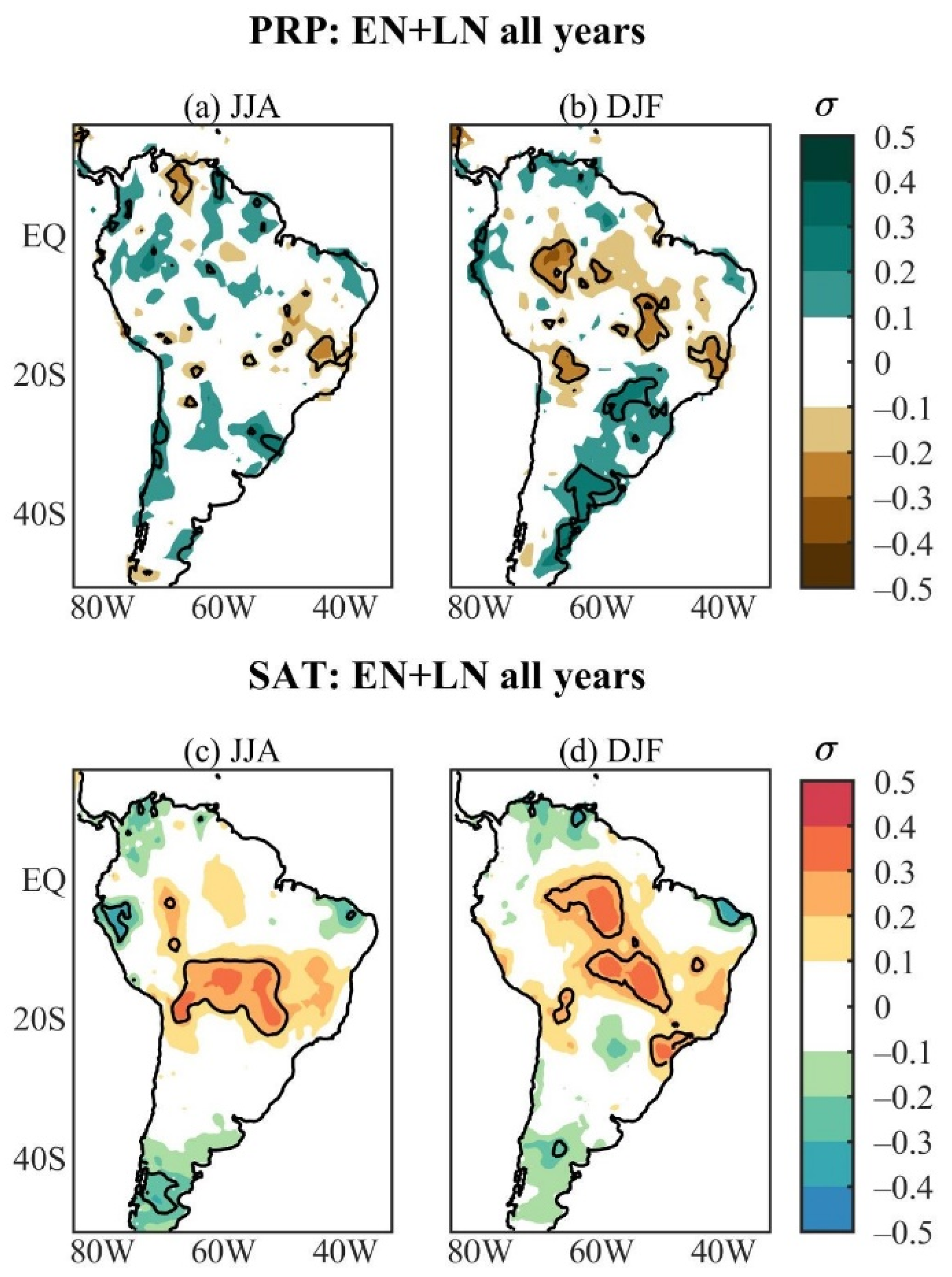
3.1. Nonlinear PRP and SAT Responses to ENSO during the 1901–2014 Period

Figure 1 shows the austral winter and summer nonlinear PRP and SAT responses to ENSO events during the 1901–2014 period. Significant nonlinear PRP anomalies are found in small scattered areas in western Venezuela (negative) as well as southeastern (negative) and southern (positive) Brazil during JJA; negative anomalies are observed in relatively larger areas of central South America, from northwestern to southeastern Brazil around 20° S, southwestern Bolivia, and positive ones in central-southeastern Brazil (east of 60° W) and central-eastern Argentina during DJF (Figure 1a,b). Regarding the SAT, the significant nonlinear anomalies are dominantly positive and found in the central South American sector extending from 10° S to 20° S during JJA and from the central Amazon to southeastern Brazil during DJF (Figure 1c,d). During DJF, the opposite sign PRP and SAT anomalies in central South America are consistent. The magnitude of the significant nonlinear PRP and SAT anomalies varies from 0.1 to 0.2 SD units in both seasons. Thus, considering all ENSO events over the period in which the climatologies are based, the nonlinear PRP and SAT responses to the ENSO are weak in South America (Figure 1). This can be the main reason why this aspect of the ENSO responses in South America has been overlooked.

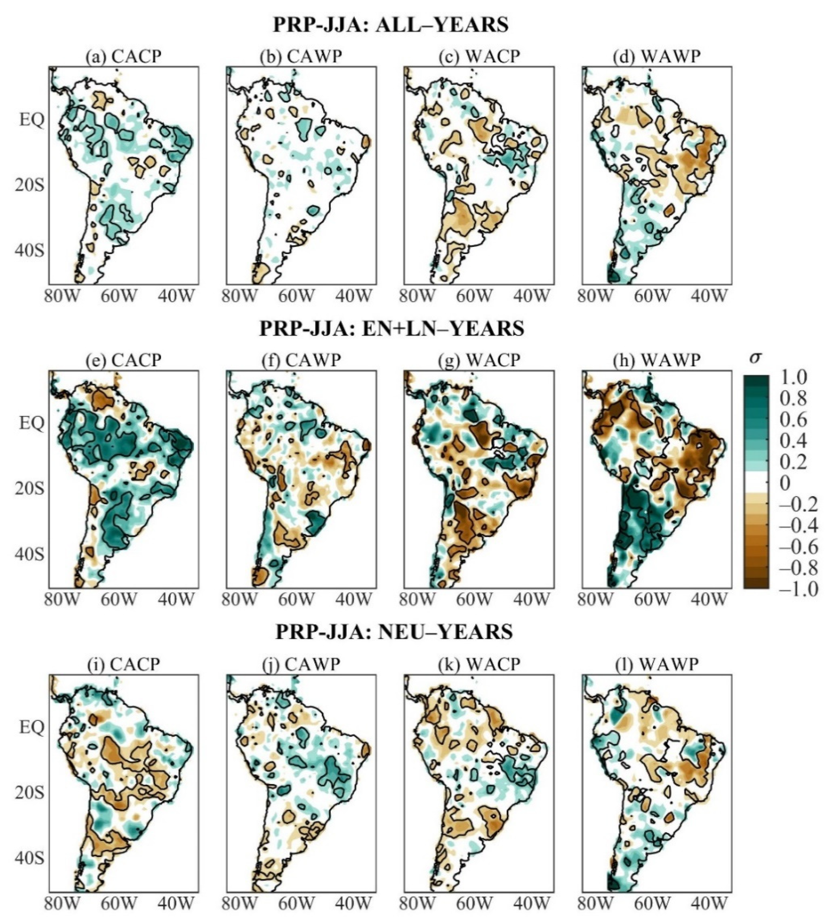
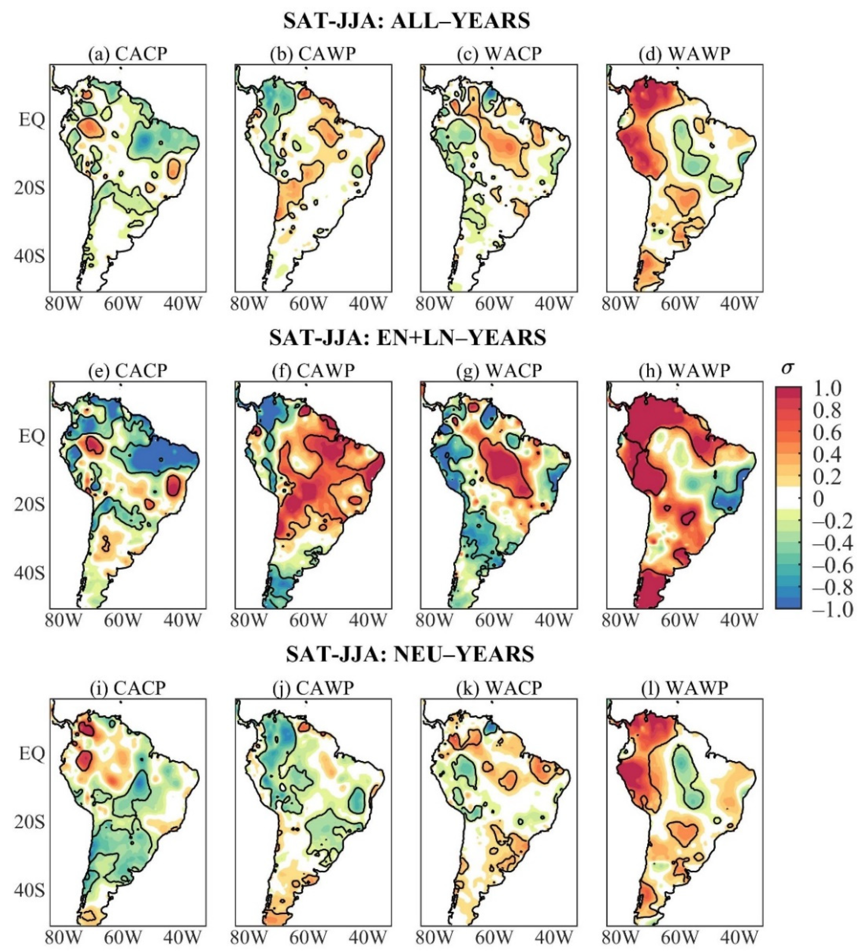
3.2. Austral Winter PRP and SAT Composites Stratified by Mean States: ALL-, EN + LN-, and NEU-Years

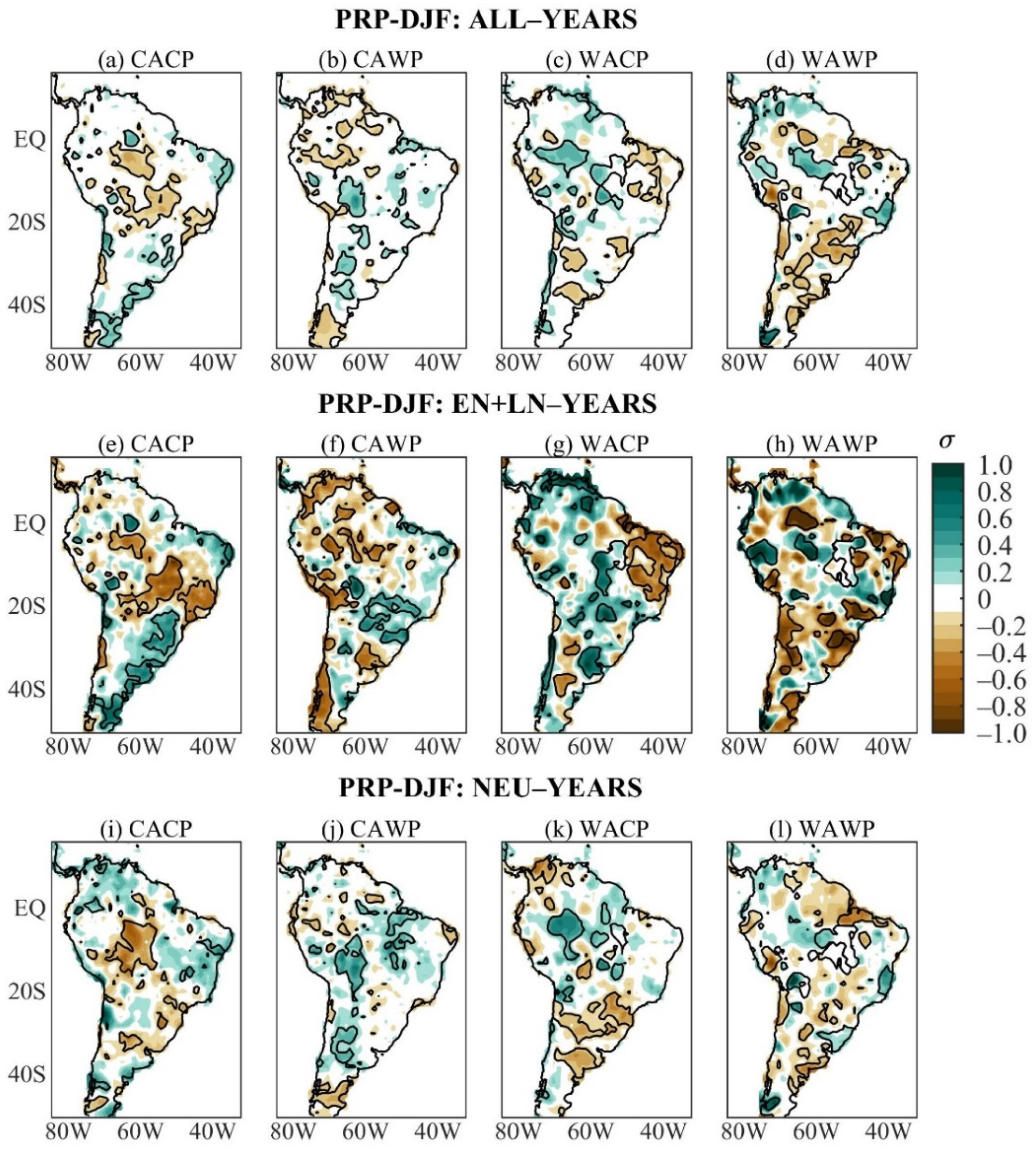
3.2.1. PRP Anomaly Patterns

The austral winter PRP anomaly composites of ALL-years of the four mean states show remarkable differences among them (Figure 2a–d). During the CACP, significant positive mean PRP anomalies show up in areas of the 5° N–15° S band, and the akin negative PRP anomalies appear in small scattered areas in western South America around 20° S, as well as in northern and central-eastern South America (Figure 2a). During the CAWP, significant mean PRP anomalies occur in small areas, being negative in western South America (northern Peru, northwestern Bolivia, south of 35° S) and in the extreme northern and northeastern areas of Brazil, and are positive in equatorial Brazil east of 60° W and southern Brazil (Figure 2b). Otherwise, the WACP mean state features significant negative mean PRP anomalies in several areas of South America west of 50° W, spread to the south of 20° S and the southern and southeastern Amazon; the akin positive PRP anomalies are centered at 15° S in central-eastern Brazil (Figure 2c). Meanwhile, significant negative mean PRP anomalies extend in central-eastern South America east of 65° W and north 25° S as well as small areas of equatorial South America, and the counterpart positive PRP anomalies appear in small areas of South America to the south of 20° S, including northwestern Peru and Suriname during WAWP (Figure 2d).

The austral winter nonlinear PRP anomaly composites stratified by the mean states are given in Figure 2e–h. Rather than reduced anomalies as for nonlinear PRP anomaly composite of all ENSO events of the study period (Figure 1a), similarities between the austral winter PRP composites of EN + LN- and ALL-years during each mean state are evident, with larger magnitudes of the nonlinear anomalies (Figure 2a–h). Further, more extensive and better-organized significant nonlinear than mean PRP anomalies are evident for some mean states and regions (Figure 2a–h). These are the cases of the positive nonlinear PRP anomalies in large areas of South America during the CACP (Figure 2e), the negative nonlinear PRP anomalies in northwestern and central-eastern South America, and the positive ones in most of 20° S–38° S sector of South America during the WAWP (Figure 2h). The ALL and EN + LN composites of the PRP anomalies show similarities during the WACP, except in southern and central-eastern Brazil, with significant negative mean and nonlinear PRP anomalies, respectively (Figure 2c,g). These results indicate that the ENSO variability contributes to the austral winter mean PRP anomalies in different ways depending on the mean state.

The austral winter NEU PRP anomaly composites stratified by the mean states are illustrated in Figure 2i–l. The three composites (ALL, EN + LN, NEU) show some common features with smaller magnitudes of the NEU anomalies depending on the mean states. Nonetheless, there are situations with more accentuated NEU PRP anomalies. Significant negative NEU PRP anomalies are found in central, tropical South America, along the 20° S, 30° S–40° S sector, and the positive ones in a small area of eastern Venezuela during the CACP (Figure 2i). The areal extension of the negative NEU PRP anomalies contrasts with small scattered areas in western South America around 20° S, and central-eastern South America encompassing the significant negative mean and nonlinear PRP anomalies (Figure 2a,e,i). Nonetheless, the dry area in northern South America noted in the ALL and EN + LN composites is not defined for the NEU composite. In addition, the expressive anomalous wetness in large extensions of the tropical South American belt of the ALL and EN + LN composites contrasts with reduced positive NEU PRP anomalies or significant negative NEU PRP anomalies in this region (Figure 2a,e,i). Thus, comparisons of the three composites (ALL, EN + LN, and NEU) indicate that the ENSO nonlinearities strongly modulate the mean PRP anomalies during the CACP. This is also confirmed by comparing the pattern correlations between ALL and EN + LN composites as well as between ALL and NEU composites of 0.91 and 0.27, respectively (

Table 3. Austral winter pattern correlations for PRP between ALL and EN + LN composites and between ALL and NEU composites in each mean state.

Mean State	ALL × EN + LN	ALL × NEU
CACP	0.91	0.27
CAWP	0.60	0.71
WACP	0.77	0.70
WAWP	0.70	0.82

).

During the CAWP, the significant negative NEU PRP anomalies occur in almost all of the small areas with the same sign mean PRP anomalies, plus areas in southern Brazil and Uruguay, and the positive NEU PRP anomalies appear in central Venezuela, the central Amazon (around 60° W), central-eastern South America (7° S–20° S), and southern Bolivia (Figure 2b,j). The opposite sign significant NEU and nonlinear PRP anomalies contrast in eastern South America between 10° S and 30° S and in western South America around 20° S, and justify the reduced mean PRP anomalies (Figure 2b,f,j). As such, the ENSO- and ENSO-neutral-years modulate the mean PRP anomalies during CAWP (Figure 2b,f,j). This is confirmed by comparable pattern correlations between ALL and EN + LN composites and between ALL and NEU composites of 0.60 and 0.71, respectively (Table 3).

Significant negative NEU PRP anomalies appear in small areas along two paths, one in northern South America, and the other from southeastern Colombia to northeastern Brazil across central and southeastern Amazonia, subtropical South America (western South America, part of southern Brazil), and the positive ones in central-eastern Brazil during WACP (Figure 2k). Except for those in northern South America, these anomalies have correspondences with mean PRP anomalies, whereas the opposite sign nonlinear and NEU PRP anomalies defined reduced mean PRP anomalies in northern South America (Figure 2g,k). Therefore, the ENSO- and ENSO-neutral-years determine the mean PRP anomalies during WACP (Figure 2c,g,k), as also indicated in Table 3 with pattern correlations between ALL and EN + LN composites and between ALL and NEU composites of 0.77 and 0.70, respectively

During the WAWP, the significant negative NEU PRP anomalies in central-eastern South America (5° S–18° S) are less extensive than the negative mean and nonlinear PRP anomalies (Figure 2d,h,l). Thus, the ENSO- and ENSO-neutral-years have contributed to the mean PRP anomaly pattern (Figure 2d,h,l). Table 3 shows pattern correlations between ALL and EN + LN composites and between ALL and NEU composites of 0.70 and 0.82, respectively.

3.2.2. SAT Anomaly Patterns

Austral winter SAT composites of ALL-years show remarkable differences among the four mean states (Figure 3a–d). During the CACP, significant mean anomalous cooling occurs in large areas of tropical South America (north coast, the eastern Amazon, northeast Brazil, southern Bolivia, Paraguay, and southern Brazil), and scattered areas of western South America north of 20° S, while the akin warming appears in reduced areas of western equatorial South America and south of northeast Brazil (Figure 3a). During the CAWP, the significant negative mean SAT anomalies extend from northern Colombia to southern Peru. The positive ones are in central Bolivia, north of Chile, the eastern Amazon, and northeast Brazil’s east coast (Figure 3b). During the WACP, significant positive mean SAT anomalies appear in the sector from southeastern Colombia to central-western Brazil, small areas of southeastern and northern Brazil, and the negative ones in eastern Venezuela and along western South America (equator–30° S) (Figure 3c). The WAWP/ALL composite features significant positive mean SAT anomalies along western South America from Venezuela to southern Peru, in a small area in subtropical South America (part of Paraguay, southern Brazil, and central-eastern Argentina), southern South America to the south of 40° S, and the opposite sign SAT anomalies appear from the central Amazon to southeastern Brazil (Figure 3d).

The austral winter nonlinear SAT anomaly composites stratified by the mean states are disclosed in Figure 3e–h. These anomalies are stronger and more extensive than those obtained considering all ENSO events during the study period (Figure 1c). As for the PRP, the austral winter SAT composites of ALL- and EN + LN-years of each mean state show similarities, with larger magnitudes of the nonlinear SAT anomalies (Figure 3a–h). This is conspicuous for the CACP composites (Figure 3a,e). Regarding the mean SAT anomalies during the CAWP, the significant negative nonlinear SAT anomalies appear in a slightly narrower band in western tropical South America and southern South America, and the positive ones appear in a larger tropical area (Figure 3b,f). Similarities are also noticeable during WACP between ALL and EN + LN SAT composites, but the significant negative nonlinear SAT anomalies over western South America extend meridionally from central Colombia to central-eastern Argentina (Figure 3c,g). The WAWP/ALL and WAWP/EN + LN SAT composites also present similar patterns, but the significant positive nonlinear SAT anomalies are more extensive in northern South America and less extensive in subtropical South America, and the negative ones are limited to the east coast of Brazil (5° S–25° S) (Figure 3d,h).

The austral winter NEU SAT composites stratified by the mean states are given in Figure 3i–l. During the CACP, significant negative NEU SAT anomalies occur in central South America between 5° S and 20° S, most of South America between 20° S and 38° S, and the positive ones are found in two small areas, with one in western Colombia and the other in northern Peru (Figure 3i). Both positive areas have correspondences with those in the ALL composite, and that in western Colombia with the EN + LN composite (Figure 3a,i). Comparisons among ALL, EN + LN, and NEU composites suggest that the nonlinear SAT anomalies are more crucial in defining the mean SAT anomalies during CACP (Figure 3a,e,i). This is confirmed in

Table 4. Austral winter pattern correlations for SAT between ALL and EN + LN composites and between ALL and NEU composites in each mean state.

Mean State	ALL × EN + LN	ALL × NEU
CACP	0.93	0.54
CAWP	0.84	0.72
WACP	0.88	0.79
WAWP	0.88	0.90

with the pattern correlations between ALL and EN + LN composites and between ALL and NEU composites of 0.93 and 0.54, respectively.

During the CAWP, significant negative NEU SAT anomalies extend from northern Colombia/western Venezuela to 20° S, part of northeast Brazil, part of central-western Brazil, southeastern and southern Brazil, and the positive ones occur in the extreme south of South America (Figure 3j). The negative NEU SAT anomalies in western tropical South America are more extensive than the corresponding mean and nonlinear SAT anomalies (Figure 3b,f,j). For this mean state, the mean SAT anomalies are combinations of the NEU and nonlinear SAT anomalies, but the nonlinear SAT anomalies modulate the anomalous warming in central Bolivia, north of Chile, the eastern Amazon, and along the east coast of northeast Brazil (Figure 3b,f,j). The pattern correlations between ALL and EN + LN composites and between ALL and NEU composites of 0.84 and 0.72, respectively, are comparable (Table 4).

During the WACP, the NEU and ALL SAT composites show similarities, but with the more horizontal structure of the significant NEU SAT anomalies such that the positive values occur in reduced areas of northwestern South America, the southeastern Amazon, northern of northeast Brazil, and subtropical eastern South America, and the negative ones appear in western South America between 5° S and 20° S (Figure 3c,k). For this mean state, the mean SAT anomalies seem to be mostly modulated by the nonlinear anomalies, particularly the anomalous cooling along western South America and the anomalous warming from southeastern Colombia to central-western Brazil (Figure 3c,g). However, the pattern correlations between ALL and EN + LN composites and between ALL and NEU composites of 0.88 and 0.79, respectively, are comparable (Table 4). The WAWP/ALL and WAWP/NEU anomaly patterns are very similar but with smaller magnitudes of the NEU SAT anomalies (Figure 3d,l). In fact, pattern correlations between ALL and EN + LN composites and between ALL and NEU composites of 0.88 and 0.90, respectively, are very close (Table 4).

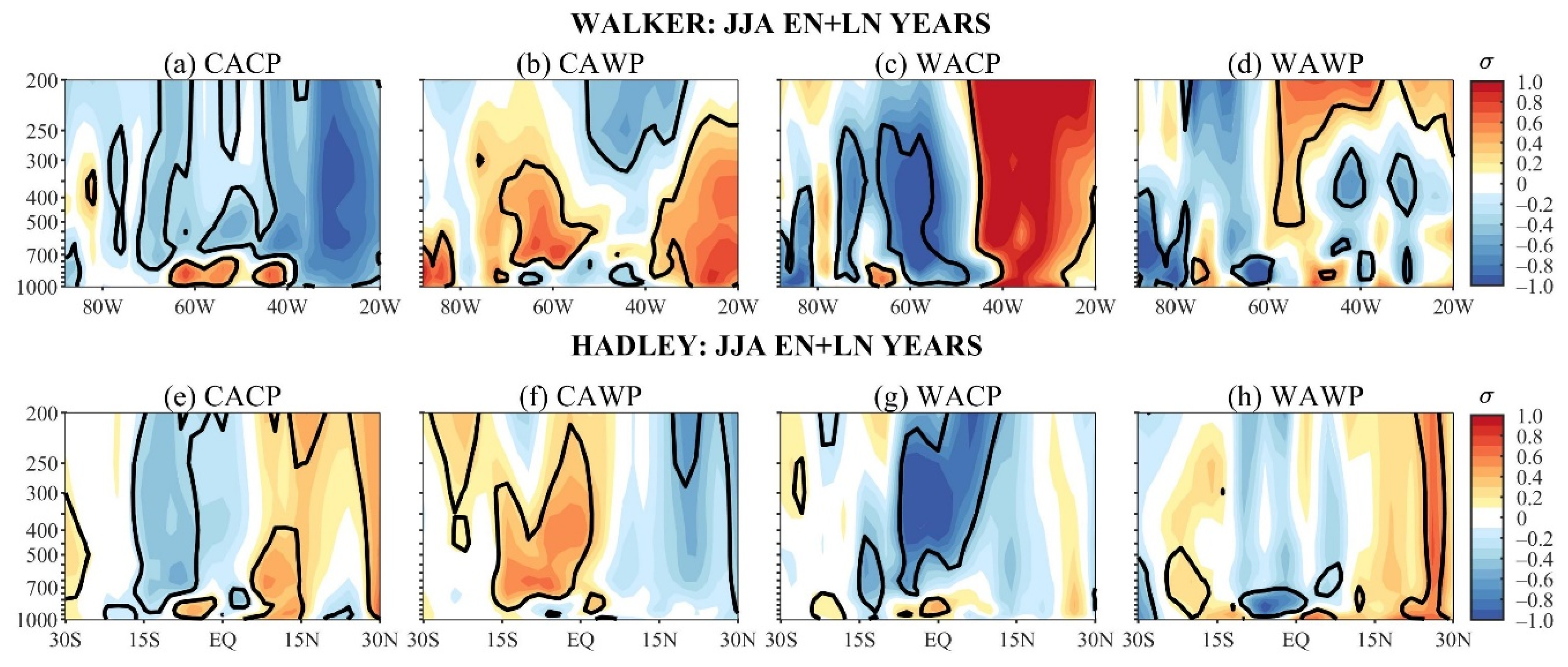
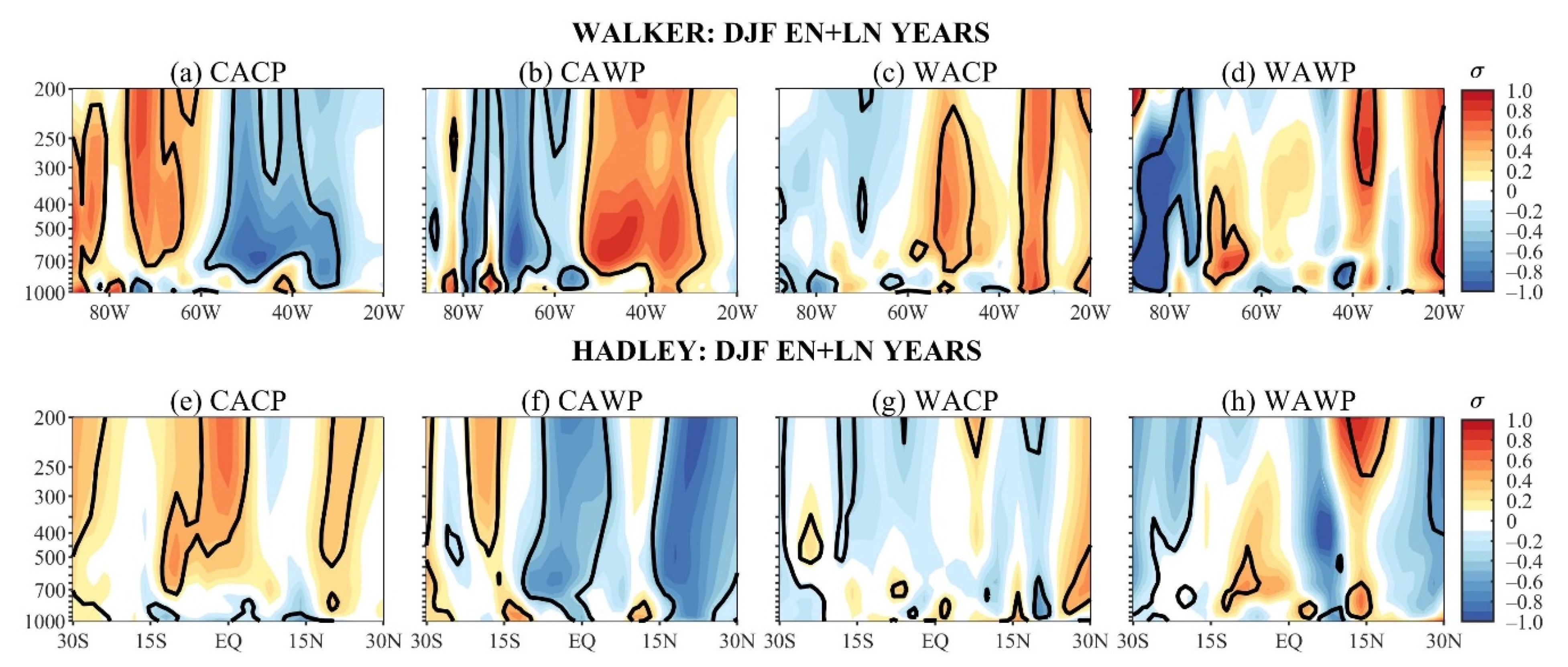
3.2.3. WVEL and HVEL Anomaly Patterns

The composites of the WVEL and HVEL anomalies over EN + LN-years of each mean state, and the corresponding composites over ALL- and NEU-years, generally show similar patterns. As such, only the WVEL and HVEL composites over EN + LN-years are presented and compared with the corresponding PRP and SAT composites.

During the CACP, the significant negative nonlinear WVEL anomalies (upward motion) occur in most tropospheric levels in the 80° W–20° W, with the largest anomalies at 30° W (Figure 4a). This ascending motion (Figure 4a) agrees with the nonlinear anomalous wetness in the 5° N–15° S sector in South America (Figure 2e), and nonlinear anomalous cooling in eastern South America east of 60° W and north of 15° S (Figure 3e). Still, significant positive nonlinear HVEL anomalies occur north of 7° N (descending motion) and the negative ones between 5° S and 17° S (ascending motion) (Figure 4e). These HVEL anomalies are part of a regional anomalous meridional cell, which is consistent with nonlinear anomalous dryness over northwestern Venezuela and the nonlinear anomalous wetness in the South American area between 5° N and 15° S and west of 60° W (Figure 2e and Figure 4e). In this South American sector, nonlinear SAT anomalies show more horizontal structure, but the prevailing negative values (Figure 3e) are consistent with the meridional cell’s rising branch (Figure 4e).

During the CAWP, the significant positive nonlinear WVEL anomalies (downward motion) occur in the 70° W–55° W sector from 700 hPa to 400 hPa and in the 40° W–15° W sector in most tropospheric levels (Figure 4b). These prevailing downward motions in most South American longitudes along 6° S is coherent with the anomalous warming of most of tropical South America, except for a narrow, meridional area in its western side (Figure 3f). Additionally, the downward motion over northeast Brazil longitudes justifies the nonlinear negative PRP anomalies in this region (Figure 2f and Figure 4b). The CAWP/EN + LN HVEL composite discloses an anomalous descending motion from lower to middle tropospheric levels between 5° N and 17° S and to the south of this latitude from middle to upper tropospheric levels (Figure 4f). This downward motion further justifies the southward extension of anomalous warming in tropical South America, particularly to the west of 60° W (Figure 3f and Figure 4f).

The WACP/EN + LN WVEL composite shows a well-defined anomalous east–west cell, with its rising and sinking branches, respectively, in the 80° W–50° W and 50° W–20° W bands (Figure 4c), which seem to be eastward displaced by 10° in longitude about the maximum anomalous cooling and warming along 6° S of the corresponding EN + LNSAT composite (Figure 3g). In addition, for the corresponding HVEL composite, the significant negative anomalies (upward motion) in most tropospheric levels in the 5° N–15° S sector justify the negative SAT anomalies along the west coast of South America (Figure 3g and Figure 4g). Nevertheless, the WACP/EN + LN PRP composite presents complex horizontal structures so that consistencies with the anomalous east–west and north–south cells are not obvious (Figure 2g and Figure 4c,g).

Consistencies among WAWP/EN + LN PRP, SAT, and WVEL composites are not evident (Figure 2h, Figure 3h and Figure 4d). During WAWP, significant negative nonlinear HVEL anomalies prevail in the equator–10° S sector (ascending motion) and the positive ones in the 15° S–25° S band (descending motion) (Figure 4h). This descending motion to the south of 15° S and the nonlinear anomalous warming along western South America are consistent (Figure 3h and Figure 4h). However, the ascending motion to the north of 10° S and the positive nonlinear SAT anomalies are not consistent. The inconsistencies seem to be due to the small number of ENSO events during the WAWP mean state.

3.3. Austral Summer PRP and SAT Composites Stratified by Mean States: ALL-, EN + LN-, and NEU-Years

3.3.1. PRP Anomaly Patterns

The austral summer PRP anomaly patterns stratified by the mean states are illustrated in Figure 5a–d. During CACP, CAWP, and WACP, comparisons with the maps shown in Kayano et al. [29] indicate that the inclusion of three additional years implies only small differences. During the CACP, significant negative mean PRP anomalies extend in areas from the central Amazon (around 60° W) to southeastern Brazil, and the positive ones appear in small areas of equatorial (around 62° W) and southern Brazil, eastern of Brazil north of 12° S, and along the east coast of South America from central-eastern Argentina to 50° S (Figure 5a). Meanwhile, during the CAWP, significant negative mean PRP anomalies occur in small scattered areas in the South American sector north of 10° S and west of 58° W, southern South America (40° S–50° S), and the positive ones show up in reduced areas in eastern equatorial South America (around 50° W), from northern Bolivia to central Argentina (Figure 5b). At the same time, during the WACP, significant positive mean PRP anomalies appear in the western and southeastern Amazon (7° S–20° S band centered at 55° W), and the negative ones in areas of northeast Brazil west of 40° W, southern Brazil, and central Argentina (Figure 5c). During the WAWP, significant positive mean PRP anomalies occur in the equator–22° S sector, highlighting a large area from the central to eastern Amazon, plus two small areas around 22° S (one in southeastern Brazil, and western South America), and the negative ones in western South America around 15° S, equatorial South America just to the west of 60° W, and small scattered areas to the south of 22° S (Figure 5d). The sign reversal of the mean PRP anomalies in western tropical South America between the WACP (positive) and CAWP (negative) during DJF reported by Kayano et al. [29] is also noted here. They argued that this sign reversal is due to a regional Walker cell’s multidecadal connection between the Atlantic and Pacific [23,24,25]. Still, for the WACP, the positive mean PRP anomalies over the western Amazon are consistent with the previous finding on the increase of PRP over the 1979–2015 period [39,40].

The austral summer composites of the nonlinear PRP anomalies stratified by the mean states are given in Figure 5e–h. In this season, it is interesting to note the similarities between the nonlinear PRP anomaly patterns of the ENSO-years of the study period and the CACP mean state (Figure 1b and Figure 5e). Thus, the PRP nonlinearity associated with ENSO variability during the CACP strongly modulates the PRP nonlinearity over the study period. Consequently, the PRP anomaly composites of the ALL- and EN + LN-years of the CACP mean state are very similar (Figure 5a,e).

During the CAWP, the EN + LN and ALL PRP anomaly composites show similarities in the South American sector to the north of 10° S, except for better defined significant negative nonlinear PRP anomalies in the western and central Amazon (Figure 5b,f). Still, during the CAWP, significant negative nonlinear PRP anomalies occur in small areas of northern Chile, southern Peru, western Uruguay and adjacent Argentina, western South America to the south of 30° S, and the positive ones occur in areas of southern Bolivia, Paraguay, central-western, southeastern, and southern Brazil (Figure 5f). For the WACP, the significant positive nonlinear PRP anomalies appear in some scattered areas in most of South America west of 50° W, except for two small areas between 30° S and 40° S, and the negative ones extend over northeast Brazil (Figure 5g). This negative area in northeast Brazil has correspondence with that in the CAWP/ALL composite (Figure 5c,g). The WAWP/EN + LN and WAWP/ALL composites of the PRP anomalies show similar patterns, except for larger magnitudes of the nonlinear anomalies (Figure 5d,h).

The austral summer PRP anomaly composites for NEU-years stratified by the mean states are given in Figure 5i–l. During the CACP, the main feature is the significant negative NEU PRP anomalies in the central Amazon (center at 10° S; 65° W), which is slightly southward extended in relation to that of the ALL composite (Figure 5a,i). Considering the ALL, EN + LN, and NEU PRP anomaly composites, it is clear that the ENSO nonlinearity is crucial in defining the mean PRP anomaly pattern during the CACP (Figure 5a,e,i). In fact, the pattern correlations between ALL and EN + LN composites and between ALL and NEU composites of 0.90 and 0.50, respectively, confirm this aspect (

Table 5. Austral summer pattern correlations for PRP between ALL and EN + LN composites and between ALL and NEU composites in each mean state.

Mean State	ALL × EN + LN	ALL × NEU
CACP	0.90	0.50
CAWP	0.75	0.70
WACP	0.72	0.72
WAWP	0.77	0.82

).

During the CAWP, significant positive NEU PRP anomalies appear in small areas of central-eastern South America, from northern Bolivia to central Argentina, and negative ones between 40° S and 50° S (Figure 5j). Comparisons of the ALL, EN + LN, and NEU anomaly composites for this mean state suggest that most features of the ALL anomaly composite in the South American sector north of 10° S and west of 58° W are modulated by the ENSO nonlinearities, but elsewhere the neutral-ENSO-years seem to be dominant (Figure 5b,f,j). Pattern correlations between ALL and EN + LN composites and between ALL and NEU composites of 0.75 and 0.70, respectively, indicate that both EN + LN and NEU PRP anomalies define the mean PRP anomalies (Table 5).

During the WACP, significant positive NEU PRP anomalies occur in the western and southeastern Amazon, and the negative ones appear in areas of southern Brazil and central Argentina. Analyzing the three composites (ALL, EN + LN, and NEU) of the WACP mean state, similarities between the NEU and the other two composites are identified in specific areas. They refer to the positive values in the western Amazon and negative ones in southern Brazil and central Argentina noted for NEU and ALL composites; the positive values in the southeastern Amazon and the negative ones in northeast Brazil are noted for the NEU and EN + LN composites (Figure 5c,g,k). Both EN + LN and NEU PRP anomalies determine the mean PRP anomalies (Table 5).

For the WAWP, significant positive NEU PRP anomalies show up in the southeastern Amazon (area centered at 10° S; 55° W), two small areas along 18° S (western Bolivia, eastern Brazil), and the negative ones occur in equatorial eastern South America (around 50° W) (Figure 5l). These areas also appear in the ALL PRP composite (Figure 5d), but outside these areas, the NEU anomalies are quite reduced and the similarities are more evident between the ALL and EN + LN composites. Thus, except for the mentioned significant NEU PRP anomalies, the mean PRP anomalies are strongly modulated by the ENSO variability during WAWP (Figure 5d,h,l). However, the pattern correlations between ALL and EN + LN composites and between ALL and NEU composites of 0.77 and 0.82, respectively, are comparable (Table 5).

3.3.2. SAT Anomaly Patterns

The austral summer SAT anomaly composites of ALL-years of the four mean states are given in Figure 6a–d. They exhibit differences among them, but similarities with the corresponding austral winter composites, particularly in areas north of 20° S, are apparent (Figure 3a–d and Figure 6a–d). During the CACP, significant negative mean SAT anomalies appear in northern South America, the eastern Amazon, northeast Brazil, Paraguay, southern Brazil, southern South America south of 35° S, and narrow areas along the west coast of South America from 5° S to 35° S (Figure 6a). During the CAWP, significant negative mean SAT anomalies extend from northern Colombia to southern Peru, from western-southeastern Brazil to northeastern Argentina, and northeast Brazil, with the positive ones occurring from the western Amazon to central-western Brazil and adjacent Bolivian areas, part of southeastern Brazil and extreme southern South America (Figure 6b). Meanwhile, during the WACP, significant positive mean SAT anomalies show up in northwestern South America, northeast Brazil, and southeastern Brazil, and the negative ones appear in western South America from the equator to 25° S. On the other hand, the austral summer and winter SAT anomaly composites of ALL-years during the WAWP mean state show similar patterns, except for the occurrence of the significant positive mean SAT anomalies in northeast Brazil and their absence in southern South America during summer (Figure 3d and Figure 6d).

The austral summer nonlinear SAT anomaly composites for each mean state are shown in Figure 6e–h. These and ALL-year composites exhibit quite similar features with stronger nonlinear SAT anomalies (Figure 6a–h). In particular, the ALL and EN + LN SAT composites during the CACP show striking similarities (Figure 6a,e). During the CAWP, besides the similar patterns of the ALL and EN + LN SAT composites, the significant nonlinear SAT anomalies present less horizontal structure, highlighting the positive area in central South America limited approximately at the equator, 25° S, 70° W, 50° W (Figure 6b,f). During the WACP, regarding the mean SAT anomalies, significant positive nonlinear SAT anomalies are more extensive in the area from the western to central-southeastern Amazon and more intense over northeast Brazil and southeastern Brazil, while the negative ones in western South America are less extensive, remaining north of 18° S (Figure 6c,g). During the WAWP, the ALL and EN + LN SAT composites also exhibit similarities, such that the significant positive nonlinear SAT anomalies are more extensive in northeastern and subtropical South America, and the negative ones are less extensive, being limited to two small areas (the northwestern Amazon and central South America around 20° S (Figure 6d,h).

The austral summer NEU SAT composites stratified by the mean states are shown in Figure 6i–l. During the CACP, significant negative NEU SAT anomalies appear in small scattered areas along the west coast of South America south of 25° S, southeastern Brazil, and the southeastern Amazon (Figure 6i). Considering the three composites for this mean state, it is obvious that the ENSO-years strongly define the mean SAT anomalies during CACP (Figure 6a,e,i). This is confirmed by the pattern correlations between ALL and EN + LN composites and between ALL and NEU composites of 0.94 and 0.61, respectively (

Table 6. Austral summer pattern correlations for SAT between ALL and EN + LN composites and between ALL and NEU composites in each mean state.

Mean State	ALL × EN + LN	ALL × NEU
CACP	0.94	0.61
CAWP	0.86	0.70
WACP	0.89	0.88
WAWP	0.88	0.89

).

The CAWP/NEU SAT composite presents significant negative SAT anomalies in most of tropical South America north of 20° S, except for areas in central, northern, and northeastern South America, and the positive ones appear in the east coast of South America to the south of 35° S (Figure 6j). The negative NEU SAT anomalies along western and eastern tropical South America north of 20° S overlap the same sign mean SAT anomalies (Figure 6b,j). As such, the mean SAT anomalies during CAWP result from a combination of the NEU and nonlinear SAT anomalies. The last ones are important in central South America (Figure 6b,f,g). The pattern correlations between ALL and EN + LN composites and between ALL and NEU composites of 0.86 and 0.70, respectively, are comparable (Table 6).

During the WACP, significant positive NEU SAT anomalies appear in small areas of northwestern, northeastern, and southwestern South America, as well as central-western Brazil (south of 20° S), and the negative ones occur from northern Peru to Bolivia (Figure 6k). The positive areas north of 20° S occur in the three composites of this mean state (Figure 6c,g,k). Therefore, the mean SAT anomaly pattern during WACP is due to both ENSO and ENSO neutral years (Figure 6c,g,k). The WAWP/NEU and WAWP/ALL SAT composites show similar patterns but with smaller magnitudes of the NEU SAT anomalies (Figure 6d,l). For the WAWP, the similarities among the ALL, EN + LN, and NEU composites indicate that the corresponding mean SAT anomaly composite results from combinations of the nonlinear and NEU SAT anomalies (Figure 6d,h,l). For WACP and WAWP, Table 6 shows almost the same magnitude of the pattern correlations between ALL and EN + LN composites and between ALL and NEU composites.

3.3.3. WVEL and HVEL Anomaly Patterns

As for the austral winter, only the WVEL and HVEL composites over EN + LN-years are presented and compared with the corresponding PRP and SAT composites

The CACP, CAWP, and WAWP of the WVEL anomaly composites over the EN + LN-years feature a significant anomalous east–west dipole along 6° S with the separation line of the nodes approximately at 60° W (Figure 7a–c). During the CACP, this dipole features its sinking and rising branches, respectively, to the west and east of 60° W (Figure 7a), and at the same time, significant positive nonlinear HVEL anomalies occur in the 5° N–15° S band (Figure 7e). Therefore, the descending motion occurs to the west of 60° W and between 5° N and 15° S and is consistent with the negative nonlinear PRP anomalies in the central Amazon to the west of 60° W during CACP (Figure 5e and Figure 7a,e). On the other hand, the ascending motion to the east of 60° W is concordant with the negative nonlinear SAT anomalies in the eastern Amazon and northeast Brazil (Figure 6e and Figure 7a).

During the CAWP, the dipole presents its rising and sinking branches, respectively, in the western and eastern nodes (Figure 7b). This anomalous rising–sinking cell is consistent with the nonlinear anomalous cooling over western South America (northern Colombia to southern Peru), and the akin warming in central South America (Figure 6f and Figure 7b). The associated HVEL anomaly composite indicates an upward motion at most tropospheric levels in the 5° N–12° S band, and a downward motion in the 12° S–17° S (Figure 7f). The ascending motion to the north of 12° S is consistent with nonlinear anomalous cooling in Colombia and the descending motion between 12° S and 17° S is consistent with nonlinear anomalous warming and dryness in central South America west of 60° S (Figure 6f and Figure 7f).

During the WACP, the nodes of the east–west dipole of the nonlinear WVEL anomalies have the same signs as those of that during CAWP, but with weaker anomalies (Figure 7b,c). During the WACP, the maximum descending motion of the eastern node appears in longitudes (just to the east of 60° W and 40° W) of anomalously warmed areas in the central-southeastern Amazon and northern of northeast Brazil, with this last area also presenting anomalous dryness (Figure 5g, Figure 6g and Figure 7c). This confirms the consistencies of the nonlinear WVEL, PRP and SAT anomalies in these areas. In addition, the ascending motion of the western node and the prevailing upward motion in the equator-18° S band associated with the HVEL/EN + LN composite are in agreement with the nonlinear anomalous cooling in western South America (5° N–20° S band) (Figure 6g and Figure 7c,g).

The WAWP/EN + LN WVEL and HVEL composite do not show well-defined zonal and meridional cells (Figure 7d,h). However, there are clear indications of the consistencies of these composites and the corresponding SAT composite (Figure 6h and Figure 7d,h). In fact, the descending motion associated with the WVEL around 70° W and HVEL between the equator and 15° S is concordant with the anomalous warming in western South America (Figure 6h and Figure 7d,h). There is also a noticeable descending motion around 40° W (Figure 7d), which agrees with the predominantly nonlinear dryness and warming over northeast Brazil (Figure 5h and Figure 6h).

4. Conclusions and Summary

Recently, Kayano et al. [28,29] examined the SST, PRP, and vertical velocity mean anomaly patterns during the mean states defined by the overlapping periods of AMO and PDO phases. Nevertheless, they did not determine if the ENSO variability affects these anomaly patterns. This aspect was investigated here for WVEL, HVEL, PRP, and SAT over South America using 114 years of data (1901–2014) and considering the CACP, CAWP, WACP, and WAWP mean states. Considering the EN- and LN-years during the study period (Table 1 and Table 2), analyses were done for the austral winter and summer and based on variable anomaly composites obtained over ALL-, EN + LN-, and NEU-years in each mean state, with the corresponding anomalies referred to as mean, nonlinear, and NEU.

The nonlinear PRP and SAT anomalies considering all ENSO events during the study period are almost negligible (Figure 1). Notwithstanding, the nonlinear PRP and SAT anomalies of the mean states are not negligible, and their patterns are similar to those of the corresponding mean anomaly composites (Figure 2a–h, Figure 3a–h, Figure 5a–h and Figure 6a–h). For both seasons, the similarities between ALL and EN + LN composites are more pronounced for SAT than for PRP (Figure 2a–h, Figure 3a–h, Figure 5a–h and Figure 6a–h). However, the ALL PRP and SAT anomaly patterns also show some features of the corresponding NEU anomaly composites during the CAWP, WACP, and WAWP (Figure 2b–d, Figure 2j–l, Figure 3b–d, Figure 3j–l, Figure 5b–d and Figure 6j–l). In contrast, during both seasons of the CACP, and for both variables, the similarities between ALL and EN + LN composites and the dissimilarities between these two composites and the NEU composites are remarkable (Figure 2a,e,i, Figure 3a,e,i, Figure 5a,e,i and Figure 6a,e,i). Thus, the mean PRP and SAT anomaly patterns are strongly modulated by the ENSO years during the CACP.

Moreover, ALL, EN + LN, and NEU SAT composites of each mean state present similarities between the two analyzed seasons, implying, in general, a weak seasonal dependence of these composites; in contrast, the corresponding PRP composites show much more seasonal variations (Figure 2, Figure 3, Figure 5 and Figure 6). Additionally, consistencies between the nonlinear vertical velocity and SAT anomalies, with anomalous downward (upward) motion associated with warming (cooling), are conspicuous for both seasons and most mean states (Figure 3e,f, Figure 4a–h, Figure 6e,f and Figure 7a–h). Nevertheless, the consistencies between the nonlinear vertical velocity and PRP anomalies are less evident, except during CACP, with an anomalous downward (upward) motion associated with dryness (wetness) (Figure 2e,f, Figure 4a–h, Figure 5e,f and Figure 7a–h).

These results indicate that the ENSO- and ENSO-neutral-years affect the variable anomaly mean states in different ways depending on the season and variable. As such, the studies on the low-frequency variability should consider not only the variable mean states but also that the ENSO variability might modulate them. It is also worth recalling that the physical consistencies among variable anomaly composites guarantee the robustness of the results. Furthermore, we calculated the 200 hPa stream function composites (Figures not shown). However, after analyzing the figures, we did not find a clear signature of the Rossby-wave trains because we are dealing with the averages of the variable anomalies during ALL-, EN + LN-, and NEU-years. The Rossby-wave train pattern should appear when analyzing EN and LN events separately. From another point of view, Enfield and Mestas-Nunez [41] applying the empirical orthogonal function analysis on the global residual SST anomalies (after removing the ENSO signal), found that the first three non-ENSO modes represent the low-frequency variability modes such that the first two modes have the strongest decadal to multidecadal signature in the Pacific and the third one in the extratropical North Atlantic. These modes correspond to the PDO and AMO. So, the results here indicated that although these are non-ENSO modes, the occurrences of ENSO extremes during their phases affect the PRP and SAT mean states in South America.

The results here have an essential implication for climate studies, in which the monthly anomalies are calculated concerning monthly climatologies based on a fixed 30-year period, which generally spans over three complete decades such as 1961–1990, 1971–2000, and 1981–2010. These 30-year periods combine distinct mean states. In the present analysis, we did not deal with the nature of the ENSO nonlinearities when the nonlinear ENSO response was considered as the summation of the EN- and LN-years [32] in each mean state. Nonetheless, we are conscious that a more detailed study evaluating the ENSO nonlinearities due to types and intensities [42] is still necessary to complement the present analysis.

References

1. Ropelewski, C.F.; Halpert, M.S. Global and Regional scale precipitation patterns associated with the El Niño-Southern Oscillation. Mon. Weather Rev. 1987, 115, 1606–1626. [Google Scholar] [CrossRef] [Green Version]
2. Ropelewski, C.F.; Halpert, M.S. Precipitation Patterns Associated with the High Index Phase of the Southern Oscillation. J. Clim. 1989, 2, 268–284. [Google Scholar] [CrossRef] [Green Version]
3. Rao, V.B.; Hada, K. Characteristics of rainfall over Brazil: Annual variations and connections with the Southern Oscillation. Theor. Appl. Climatol. 1990, 42, 81–91. [Google Scholar] [CrossRef]
4. Pisciottano, G.; Díaz, A.; Cazes, G.; Mechoso, C.R. El Niño-Southern Oscillation impact on rainfall in Uruguay. J. Clim. 1994, 7, 1286–1302. [Google Scholar] [CrossRef] [Green Version]
5. Diaz, A.F.; Studzinski, C.D.; Mechoso, C.R. Relationships between precipitation anomalies in Uruguay and southern Brazil and sea surface temperature in the Pacific and Atlantic oceans. J. Clim. 1998, 11, 251–271. [Google Scholar] [CrossRef]
6. Grimm, A.M.; Ferraz, S.E.T.; Gomes, J. Precipitation Anomalies in Southern Brazil Associated with El Niño and La Niña Events. J. Clim. 1998, 11, 2863–2880. [Google Scholar] [CrossRef] [Green Version]
7. Grimm, A.; Barros, V.; Doyle, M. Climate Variability in Southern South America Associated with El Niño and La Niña Events. J. Clim. 2000, 13, 35–58. [Google Scholar] [CrossRef]
8. Kousky, V.E.; Ropelewski, C.F. Extremes in the Southern Oscillation and their Relationship to Precipitation Anomalies with Emphasis on the South American Region. Rev. Bras. Meteorol. 1989, 4, 351–363. [Google Scholar]
9. Aceituno, P. On the Functioning of the Southern Oscillation in the South American Sector. Part I: Surface Climate. Mon. Weather Rev. 1988, 116, 505–524. [Google Scholar] [CrossRef] [Green Version]
10. Kiladis, G.N.; Diaz, H.F. Global climatic anomalies associated with extremes in the Southern Oscillation. J. Clim. 1989, 2, 1069–1090. [Google Scholar] [CrossRef] [Green Version]
11. Nogués-Paegle, J.; Mechoso, C.; Fu, R.; Berbery, E.; Chao, W.; Chen, T.-C.; Cook, K.; Diaz, A.; Enfield, D.; Ferreira, R. Progress in Pan American CLIVAR research: Understanding the South American monsoon. Meteorologica 2002, 27, 1–30. [Google Scholar]
12. Zhou, J.; Lau, K.M. Principal modes of interannual and decadal variability of summer rainfall over South America. Int. J. Climatol. 2001, 21, 1623–1644. [Google Scholar] [CrossRef]
13. Barros, V.R.; Silvestri, G.E. The relation between sea surface temperature at the subtropical South-Central Pacific and precipitation in Southeastern South America. J. Clim. 2002, 15, 251–267. [Google Scholar] [CrossRef]
14. Garreaud, R.D.; Falvey, M. The coastal winds off western subtropical South America in future climate scenarios. Int. J. Climatol. 2009, 29, 543–554. [Google Scholar] [CrossRef]
15. Berman, A.L.; Silvestri, G.; Compagnucci, R.; Velasco Herrera, V. Oceanic influence on southernmost South American precipitation. Atmosfera 2012, 25, 217–233. [Google Scholar]
16. Cai, W.; McPhaden, M.J.; Grimm, A.M.; Rodrigues, R.R.; Taschetto, A.S.; Garreaud, R.D.; Dewitte, B.; Poveda, G.; Ham, Y.-G.; Santoso, A.; et al. Climate impacts of the El Niño–Southern Oscillation on South America. Nat. Rev. Earth Environ. 2020, 1, 215–231. [Google Scholar] [CrossRef]
17. Dettinger, M.D.; Battisti, D.S.; Garreaud, R.D.; McCabe, G.J.; Bitz, C.M. Interhemispheric Effects of Interannual and Decadal ENSO-Like Climate Variations on the Americas. In Interhemispheric Climate Linkages: Present and Past Climates in the Americas and their Societal Effects; Markgraf, V., Ed.; Academic Press: San Diego, CA, USA, 2001; pp. 1–16. ISBN 9780124726703. [Google Scholar]
18. Kayano, M.T.; Andreoli, R.V.; de Souza, R.A.F.; Garcia, S.R. Spatiotemporal variability modes of surface air temperature in South America during the 1951–2010 period: ENSO and non-ENSO components. Int. J. Climatol. 2017, 37, 1–13. [Google Scholar] [CrossRef]
19. Li, Y.; Li, J.; Kucharski, F.; Feng, J.; Zhao, S.; Zheng, J. Two leading modes of the interannual variability in South American surface air temperature during austral winter. Clim. Dyn. 2018, 51, 2141–2156. [Google Scholar] [CrossRef]
20. Mantua, N.J.; Hare, S.R.; Zhang, Y.; Wallace, J.M.; Francis, R.C. A Pacific Interdecadal Climate Oscillation with Impacts on Salmon Production. Bull. Am. Meteorol. Soc. 1997, 78, 1069–1079. [Google Scholar] [CrossRef]
21. Chen, S.; Song, L.; Chen, W. Interdecadal Modulation of AMO on the Winter North Pacific Oscillation-Following Winter ENSO Relationship. Adv. Atmos. Sci. 2019, 36, 1393–1403. [Google Scholar] [CrossRef]
22. Kim, D.; Lee, S.K.; Lopez, H.; Goes, M. Pacific mean-state control of atlantic multidecadal oscillation-El Niño relationship. J. Clim. 2020, 33, 4273–4291. [Google Scholar] [CrossRef]
23. McGregor, S.; Timmermann, A.; Stuecker, M.F.; England, M.H.; Merrifield, M.; Jin, F.F.; Chikamoto, Y. Recent Walker circulation strengthening and pacific cooling amplified by Atlantic warming. Nat. Clim. Chang. 2014, 4, 888. [Google Scholar] [CrossRef] [Green Version]
24. Kucharski, F.; Parvin, A.; Rodriguez-Fonseca, B.; Farneti, R.; Martin-Rey, M.; Polo, I.; Mohino, E.; Losada, T.; Mechoso, C.R. The teleconnection of the tropical Atlantic to Indo-Pacific sea surface temperatures on inter-annual to centennial time scales: A review of recent findings. Atmosphere 2016, 7, 29. [Google Scholar] [CrossRef] [Green Version]
25. Kucharski, F.; Ikram, F.; Molteni, F.; Farneti, R.; Kang, I.S.; No, H.H.; King, M.P.; Giuliani, G.; Mogensen, K. Atlantic forcing of Pacific decadal variability. Clim. Dyn. 2016, 46, 2337–2351. [Google Scholar] [CrossRef]
26. Meehl, G.A.; Hu, A.; Castruccio, F.; England, M.H.; Bates, S.C.; Danabasoglu, G.; McGregor, S.; Arblaster, J.M.; Xie, S.P.; Rosenbloom, N. Atlantic and Pacific tropics connected by mutually interactive decadal-timescale processes. Nat. Geosci. 2021, 14, 36–42. [Google Scholar] [CrossRef]
27. Maleski, J.J.; Martinez, C.J. Coupled impacts of ENSO AMO and PDO on temperature and precipitation in the Alabama–Coosa–Tallapoosa and Apalachicola–Chattahoochee–Flint river basins. Int. J. Climatol. 2018, 38, e717–e728. [Google Scholar] [CrossRef]
28. Kayano, M.T.; Andreoli, R.V.; Souza, R.A.F. El Niño–Southern Oscillation related teleconnections over South America under distinct Atlantic Multidecadal Oscillation and Pacific Interdecadal Oscillation backgrounds: La Niña. Int. J. Climatol. 2019, 39, 1359–1372. [Google Scholar] [CrossRef]
29. Kayano, M.T.; Andreoli, R.V.; Souza, R.A.F. Pacific and Atlantic multidecadal variability relations to the El Niño events and their effects on the South American rainfall. Int. J. Climatol. 2020, 40, 2183–2200. [Google Scholar] [CrossRef]
30. Cerón, W.L.; Kayano, M.T.; Andreoli, R.V.; Avila-Diaz, A.; de Souza, I.P.; Souza, R.A.F. Pacific and atlantic multidecadal variability relations with the choco and caribbean low-level jets during the 1900–2015 period. Atmosphere 2021, 12, 1120. [Google Scholar] [CrossRef]
31. He, Z.; Dai, A.; Vuille, M. The Joint Impacts of Atlantic and Pacific Multidecadal Variability on South American Precipitation and Temperature. J. Clim. 2021, 34, 7959–7981. [Google Scholar] [CrossRef]
32. Hoerling, M.P.; Kumar, A.; Zhong, M. El Niño, La Niña, and the nonlinearity of their teleconnections. J. Clim. 1997, 10, 1769–1786. [Google Scholar] [CrossRef]
33. Huang, B.; Thorne, P.W.; Banzon, V.F.; Boyer, T.; Chepurin, G.; Lawrimore, J.H.; Menne, M.J.; Smith, T.M.; Vose, R.S.; Zhang, H.M. Extended reconstructed Sea surface temperature, Version 5 (ERSSTv5): Upgrades, validations, and intercomparisons. J. Clim. 2017, 30, 8179–8205. [Google Scholar] [CrossRef]
34. Compo, G.P.; Whitaker, J.S.; Sardeshmukh, P.D.; Matsui, N.; Allan, R.J.; Yin, X.; Gleason, B.E.; Vose, R.S.; Rutledge, G.; Bessemoulin, P.; et al. The Twentieth Century Reanalysis Project. Q. J. R. Meteorol. Soc. 2011, 137, 1–28. [Google Scholar] [CrossRef]
35. Matsuura, K.; Willmott, C.J. Terrestrial Air Temperature: 1900–2017 Gridded Monthly Time Series, Version 5.01. Available online: http://climate.geog.udel.edu/~climate/html_pages/Global2017/README.GlobalTsT2017.html (accessed on 22 April 2020).
36. Schneider, U.; Becker, A.; Finger, P.; Meyer-Christoffer, A.; Ziese, M.; Rudolf, B. GPCC’s new land surface precipitation climatology based on quality-controlled in situ data and its role in quantifying the global water cycle. Theor. Appl. Climatol. 2014, 115, 15–40. [Google Scholar] [CrossRef] [Green Version]
37. Global Precipitation Climatology Centre (GPCC) Monthly Gridded Precipitation Data. Available online: https://www.esrl.noaa.gov/psd/data/gridded/data.gpcc.html (accessed on 3 May 2019).
38. Wilks, D.S. Statistical Methods in the Atmospheric Sciences, 3rd ed.; Wilks, D.S., Ed.; Academic Press: San Diego, CA, USA, 2011; ISBN 9780123850232. [Google Scholar]
39. Wang, X.Y.; Li, X.; Zhu, J.; Tanajura, C.A.S. The strengthening of Amazonian precipitation during the wet season driven by tropical sea surface temperature forcing. Environ. Res. Lett. 2018, 13, 094015. [Google Scholar] [CrossRef] [Green Version]
40. Barichivich, J.; Gloor, E.; Peylin, P.; Brienen, R.J.W.; Schöngart, J.; Espinoza, J.C.; Pattnayak, K.C. Recent intensification of Amazon flooding extremes driven by strengthened Walker circulation. Sci. Adv. 2018, 4, eaat8785. [Google Scholar] [CrossRef] [PubMed] [Green Version]
41. Enfield, D.B.; Mestas-Nuñez, A.M. Multiscale variabilities in global sea surface temperatures and their relationships with tropospheric climate patterns. J. Clim. 1999, 12, 2734–2746. [Google Scholar] [CrossRef]
42. Ashok, K.; Behera, S.K.; Rao, S.A.; Weng, H.; Yamagata, T. El Niño Modoki and its possible teleconnection. J. Geophys. Res. Ocean. 2007, 112, 1–27. [Google Scholar] [CrossRef]
Figure 1. Austral summer and winter nonlinear standardized anomaly patterns of all ENSO events during the 1901–2014 period for (a,b) PRP and (c,d) SAT. Continuous contours encompass the significant anomalies at a 90% confidence level using the Student’s t-test. The symbol σ above the colour bar means standard deviation.
Atmosphere 13 00231 g001
Figure 2. Austral winter PRP anomaly composites of ALL-years during the: (a) CACP, (b) CAWP, (c) WACP, and (d) WAWP mean states; of EN + LN-years during the: I CACP, (e) CACP, (f) CAWP, (g) WACP, and (h) WAWP mean states; of NEU-years during the: (i) CACP, (j) CAWP, (k) WACP, and (l) WAWP mean states. Continuous contours encompass the significant anomalies at a 90% confidence level using the Student’s t-test. The symbol σ above the colour bar means standard deviation.
Atmosphere 13 00231 g002
Figure 3. Austral winter SAT anomaly composites of ALL-years during the: (a) CACP, (b) CAWP, (c) WACP, and (d) WAWP mean states; of EN + LN-years during the: (e) CACP, (f) CAWP, (g) WACP, and (h) WAWP mean states; of NEU-years during the: (i) CACP, (j) CAWP, (k) WACP, and (l) WAWP mean states. Continuous contours encompass the significant anomalies at a 90% confidence level using the Student’s t-test. The symbol σ above the colour bar means standard deviation.
Atmosphere 13 00231 g003
Figure 4. Austral winter longitude vertical cross-section of the WVEL anomaly composites of EN + LN during the: (a) CACP, (b) CAWP, (c) WACP, and (d) WAWP mean states; and latitude vertical cross-section of the HVEL anomaly composites of EN + LN during the: (e) CACP, (f) CAWP, (g) WACP, and (h) WAWP mean states. Continuous contours encompass the significant anomalies at a 90% confidence level using the Student’s t-test. The symbol σ above the colour bar means standard deviation.
Atmosphere 13 00231 g004
Figure 5. Austral summer PRP anomaly composites of ALL-years during the: (a) CACP, (b) CAWP, (c) WACP, and (d) WAWP mean states; of EN + LN-years during the: (e) CACP, (f) CAWP, (g) WACP, and (h) WAWP mean states; of NEU-years during the: (i) CACP, (j) CAWP, (k) WACP, and (l) WAWP mean states. Continuous contours encompass the significant anomalies at a 90% confidence level using the Student’s t-test. The symbol σ above the colour bar means standard deviation.
Atmosphere 13 00231 g005
Figure 6. Austral summer SAT anomaly composites of ALL-years during the: (a) CACP, (b) CAWP, (c) WACP, and (d) WAWP mean states; of EN + LN-years during the: (e) CACP, (f) CAWP, (g) WACP, and (h) WAWP mean states; of NEU-years during the: (i) CACP, (j) CAWP, (k) WACP, and (l) WAWP mean states. Continuous contours encompass the significant anomalies at a 90% confidence level using the Student’s t-test. The symbol σ above the colour bar means standard deviation.
Atmosphere 13 00231 g006
Figure 7. Austral summer longitude vertical cross-section of the WVEL anomaly composites of EN + LN during the: (a) CACP, (b) CAWP, (c) WACP, and (d) WAWP mean states; and latitude vertical cross-section of the HVEL anomaly composites of EN + LN during the: (e) CACP, (f) CAWP, (g) WACP, and (h) WAWP mean states. Continuous contours encompass the significant anomalies at a 90% confidence level using the Student’s t-test. The symbol σ above the colour bar means standard deviation.
Atmosphere 13 00231 g007