The IOD–ENSO Interaction: The Role of the Indian Ocean Current’s System

Abstract

The Indian Ocean dipole (IOD) is one of the main modes characterizing the interannual variability of the large-scale ocean–atmosphere interaction in the equatorial zone of the World Ocean. A dipole manifests itself as an out-of-phase interannual fluctuation of the ocean–atmosphere characteristics in the western and eastern parts of the equatorial–tropical zone of the Indian Ocean. IOD can be a consequence of the ENSO (El Niño–Southern Oscillation) events in the Pacific Ocean, or it can be independent of them and arise due to the Indian Ocean inherent processes. Earlier, it was suggested that the generation of the long planetary waves in the Indian Ocean by the ENSO events is one of the mechanisms of the ENSO impact on the IOD. However, quite often, such a mechanism is not the case and IOD is generated itself as an independent Indian Ocean mode. We hypothesized that this generation is due to the growing oceanic disturbances, as a result of instability of the system of Indian Ocean zonal currents in the vicinity of the critical layer, in which the phase velocity of Rossby waves is equal to the average velocity of the zonal currents. In the present work, the study of the features of the formation of the critical layer in the equatorial–tropical zone of the Indian Ocean is continued using different oceanic re-analyses and standard theory of the Rossby waves. As a result of comparison of different re-analyses data with the RAMA (The Research Moored Array for African-Asian-Australian Monsoon Analysis and Prediction) measurements, the operative re-analysis ORAS5 output of European Centre for Medium-Range Weather Forecasts (ECMWF) on potential temperature, salinity, and the zonal component of the currents’ velocity for the period 1979–2018 was used. Monthly profiles of potential temperature, salinity, and the zonal component of the currents’ velocity were selected from the ORAS5 archive for the sections situated between 7.5–15.5° S and 50–100° E. From these data and for each month, using the standard theory of planetary waves, the phase velocity of the lowest baroclinic mode of the Rossby long waves was calculated and the critical layers were determined. For each critical layer, its length was calculated. The obtained time series of the length of the critical layers were compared to the variability of dipole mode index (DMI). It is shown that the majority of the cases of the IOD generation as inherent (independent on the Pacific processes) mode were accompanied by the critical layer formation in the region of interest. Usually, the critical layers occur in spring, one to two months before the onset of the positive IOD events. This indicates that the presence of instability in the system of the zonal currents can be a reason for the generation of IOD and the asymmetry of the amplitude of the dipole mode index between positive and negative events. During the extremely intense ENSO event of 1997–1998, which was accompanied by the strong IOD event, the critical layer in the equatorial–tropical zone of the Indian Ocean was absent. This ENSO event generated the oceanic planetary waves at the eastern edge of the Indian Ocean. Therefore, it is shown that the above mechanism of the ENSO–IOD interaction is a reality.

1. Introduction

The Indian Ocean dipole (IOD) is one of the main modes characterizing the interannual variability of the parameters of the large-scale interaction between the ocean and the atmosphere in the equatorial zone of the World Ocean. Dipole is also one of the leading Indian Ocean interannual modes. IOD events are manifested in the out-of-phase interannual fluctuations in the characteristics of the interaction between the ocean and the atmosphere in the western and eastern parts of the equatorial–tropical zone of the Indian Ocean [1]. Another interannual Indian Ocean basin-wide (IOBW) mode is monopole. It is orthogonal to the IOD mode [2].

IOD is characterized by three phases: neutral, positive and negative. In the neutral phase, warm water of the Western Pacific Ocean pool flowing into the Indian Ocean between the Indonesian islands maintains a warm state of the upper ocean and high sea surface temperature (SST) in the eastern equatorial zone of the Indian Ocean. Air masses rise above this region and descend into the western half of the basin, while relatively weak near surface eastward winds prevail along the equator. These winds are not strong because the SST and thermocline depth in the Western Indian Ocean differ a little bit from the SST and depth of the thermocline in the Eastern Indian Ocean. This state is close to normal and does not cause significant climate anomalies in the region [3]. In the negative IOD phase, the westerly equatorial winds intensify. It leads to a surge and, as a consequence, an increase in the concentration of warm water off the coasts of Australia and Indonesia. The depth of the thermocline in this region increases, while in the western part of the Indian Ocean, on the contrary, it decreases. This leads to increase of the zonal temperature difference in the equatorial–tropical zone of the Indian Ocean: the water is getting warmer than usual in the east and colder than in the neutral phase in the west. In its positive phase, IOD manifests itself in the anomalous sea surface cooling in the southeastern part of the equatorial–tropical zone and heating in the West and in the central part of the equatorial–tropical Indian Ocean. During this time, the westerly winds are weakening along the equator, allowing warm water to move towards Africa. A change in the wind regime leads to an anomalous rise of the thermocline in the East and its deepening in the central part of the equatorial zone of the Indian Ocean [4].

The variability in the “ocean–atmosphere” system associated with the IOD events significantly impacts the climate in the regions surrounding Indian Ocean. Usually, this variability manifests itself in the abnormal moisture transfer and the heavy rainfall (or, conversely, the abnormal droughts). Hydrometeorological anomalies accompanying the positive phase of IOD in 1961, 1994, 2006 and 2019 caused devastating floods, landslides and outbreaks of infectious diseases in East African countries [5,6,7,8], and catastrophic droughts and forest fires in Indonesia [9,10] and Australia [11]. The impact of the IOD of 2019 was particularly devastating. The season of wildfires in Australia, which began earlier than usual, is called “Black Summer”. The fire broke out in June 2019 in the forests of Northeastern Australia. By March 2020, about 180 thousand square kilometers had burned down, 59 thousand buildings were destroyed, and at least 34 people died, including 10 firefighters [12]. In East Africa, by contrast, 2019 rainfall anomalies resulted in an unusually productive rainy season, one of the strongest in a decade. This region experienced severe floods and devastating landslides, which affected more than 2.8 million people [13].

The processes of the heat redistribution within the equatorial–tropical zone of the Indian Ocean are not only of regional interest. Planetary waves generated by anomalous Indian Ocean conditions can affect a significant proportion of the Earth or even globally through the atmospheric bridge. For instance, recent studies have shown a significant link between changes in surface temperature, pressure and precipitation in the Northern and Central Eurasian region and the IOD events [14,15]. Therefore, considerable attention has been given by different authors to the study of teleconnection patterns and the regional IOD manifestations. In addition, the Indian Ocean is one of the main sources of heat for the South Atlantic Ocean.

According to the results of the modern research [16,17], two main types of IOD can be distinguished. The first type is related to the characteristics of interannual variability in the Indo-Pacific region and is described as part of the complex El Niño–Southern Oscillation (ENSO)–IOD system. This type is associated mainly with the Indian Ocean and Pacific equatorial Walker cells [18,19,20]. This relationship is confirmed by a significant (at the level of 0.55) correlation between the time series of the IOD and ENSO indices in the boreal autumn months. However, this does not answer the question as to why in some years of strong El Niño or La Niña, the IOD events do not arise at all, as for example in 2007, or do not develop as strongly as in the other years. This relationship can be explained by the fact that ENSO in some cases can generate IOD, while in the other cases, IOD is generated in the Indian Ocean without the ENSO participation [21]. The last type of variability represents the second type of IOD, which is independent of the ENSO. The existence of independent IOD events was proven back in the 2000s using a coupled general circulation model of the ocean–atmosphere system [22]. In the numerical experiments of over 50 years of model time it was demonstrated that eight IOD events occurred that were not associated with the ENSO. As the analysis of the heat budget has shown, the processes of interaction between the ocean and the atmosphere have a decisive influence on the formation of the simulated IOD events. In [23], this model result was confirmed by the observational data. The authors of this work showed that over 127 years, 65% of the IOD events occurred without the ENSO events in the Pacific Ocean, and 35% of the remaining IOD events were accompanied by the ENSO events. In addition, the existence of an independent IOD mode can explain some of the features of the regional manifestations of the ENSO–IOD system. For example, it has been suggested that IOD is more likely than ENSO to be responsible for the drought in Southeastern Australia in 2009. The IOD influence explains all of the iconic Australian droughts of the 20th century, and 11 out of 21 catastrophic wildfires since 1950 have been preceded by a positive IOD phase [24].

The existence of an independent IOD mode usually associates with the strong regional seasonal climate variability. In fact, seasonal phase synchronization is an important feature of the IOD: significant anomalies in the Indian Ocean climatic system usually appear in the early boreal summer (in June), develop in the following months, and reach a peak in October–November [25,26]. Planetary ocean waves play an important role in the generation of the IOD events. The authors of [27] described the scheme of IOD evolution on the example of the positive phase of the events IOD of 1997, 1994 and 1982 and the negative phase of the events of 1996 and 1984–1985. In this schema, anomalies that are formed in the wind field during one of the IOD phases in the western equatorial zone of the Indian Ocean generate oceanic equatorial Kelvin waves propagating eastward. Reaching the eastern boundary of the ocean, they are reflected and generate equatorially-trapped baroclinic Rossby waves propagating westward. These waves, changing the thermocline depth, switch the IOD phase to the opposite one. The results published in the paper [28] confirm that. This mechanism is very close to the mechanism of ENSO formation in the Pacific Ocean [29]. Earlier, the authors of the present work showed the important role of non-equatorial oceanic waves in the propagation of thermal anomalies in the tropical zone of the Indian Ocean in the zonal direction. We suggested that the IOD intensity and the link between the IOD events and the ENSO may be closely related to the seasonal oceanic currents’ variability in the southern equatorial–tropical zone of the Indian Ocean. Using the climatic data of the ORAS5 re-analysis on an average annual scale, it has been shown that in the vicinity of 11–12° S a critical layer is formed. In this layer, the phase speed of the Rossby waves is equal to the average velocity of the zonal currents. Here, the free Rossby waves cannot exist and must be absorbed. Concurrently, the development of instability of the system of zonal currents, which are subject to the high-magnitude seasonal variability, is possible there [30,31]. The importance of non-equatorial processes for the development of the IOD events is also confirmed by the fact that anomalies in the “ocean–atmosphere” system are not pure “equatorially trapped” because they are characterized by a pronounced asymmetry relative to the equatorial plane [32].

The purpose of this work is to study the influence of the oceanic critical layers on the IOD–ENSO system for the period of 1979–2018. It was assumed that if we consider not the average annual data averaged over the entire observation period, but take specific years and months, it is possible to distinguish the independent IOD events that arise due to the instability of the system of zonal currents in the critical layer vicinity. It is shown that most cases of the emergence of the critical layer occur during the years of positive IOD events one to two months before the development of these events. In addition, it is demonstrated that there are IOD events that do not depend on the ENSO events and a critical layer arising before these events is a plausible reason for that.

2. Materials and Methods

Operative re-analysis ORAS5 data of the European Centre for Medium-Range Weather Forecasts (ECMWF) on potential temperature, salinity and the zonal component of the current velocity for the period 1979–2018 were used. The data were taken at the nodes of a one-degree grid for the region bounded by coordinates 7.5–15.5° S and 50–100° E (Figure 1). Results obtained by the authors in the papers [33,34] show that critical layers in the Indian Ocean typically have to be formed in the vicinity of South Equatorial Current (SEC) core to the south of 8° S and up to 15° S. Associated temperature interannual variability in the upper tropical Indian Ocean layers takes place in the more broad band because of the geostrophic SEC nature [35,36,37], but we consider the processes in the currents’ system between 7.5° S and 15.5° S as one of the principal generators of the interannual temperature variations south of the equator in the tropical Indian Ocean. Just for that reason we have restricted the region of currents’ consideration by the latitudes from 7.5° S to 15.5° S. The choice of the ORAS5 re-analysis was determined by the results of comparing different re-analysis with the data of field observations of the Research Moored Array for African-Asian-Australian Monsoon Analysis and Prediction (RAMA) program [38].

Based on the data on potential temperature and salinity for each month, the average potential density at each grid point was calculated. Then, with sufficient accuracy, the Brunt–Väisälä frequency using the Gibbs-SeaWater (GSW) Oceanographic Toolbox software package in the Matlab R2017a was calculated. The phase velocity of Rossby waves was determined from the monthly average value of the Brunt–Väisälä frequency. The formula for calculating the phase velocity of the first baroclinic mode of planetary waves (Rossby waves) is derived from the basis of the following dispersion relation:

$${\omega }_n=\frac{-{\beta k}_1}{k_h^{ 2}+\frac{f^{ 2}}{{gh}_n}},$$

(1)

where ω_n—frequency of the first baroclinic mode (n = 1); f—Coriolis parameter; h_n—the equivalent depth, which determines the speed of propagation of a planetary baroclinic wave, and k_h—wave number.

$$k_h={\left(k_1^2{+k}_2^2\right)}^{\frac{1}{2}},$$

(2)

in this case k₂ = 0, that is, only zonal wave disturbances were analyzed; β—parameter describing the variation of the Coriolis parameter with latitude:

$$\beta =\frac{2\mathsf{\Omega }\cos \phi }{R},$$

(3)

where Ω = 7.29 × 10⁻⁵ s⁻¹—angular frequency of rotation of the Earth; φ—latitude; R ≈ 6370 km—radius of the Earth. The equivalent depth was determined from the following ratio:

$$h_n=\frac{N^2{H}^2}{{gn}^2\pi },$$

(4)

where H—ocean depth (it was taken for each specific profile from the re-analysis data); n—mode number (in this case, n = 1). Then, the phase velocity of the first baroclinic mode of the Rossby wave was determined from the following relation:

$$c_1=\frac{1}{k_h^{ 2}\left(k_h^{ 2}+\frac{f^{ 2}}{{gh}_1}\right)}\left(-{\beta k}_1^{ 2}\right).$$

(5)

because k_h = k₁ and k₁² for the considered long Rossby waves (wave length λ = 2π/k₁ > 1000 km) is about an order of magnitude less than the ratio f²/gh₁, then c₁ with sufficient accuracy can be written in the following form:

$$c_1=\frac{-{\beta gh}_1}{f^{ 2}}.$$

(6)

Equation (6) determines the phase velocity of long nondispersive Rossby waves. Then, using interpolation, the coordinates and depths of those points were calculated where the phase velocities of these waves are equal to the average velocities of the zonal currents. Thus, the localization of the critical layers was established: the coordinates and depth of its occurrence. An example of a critical layer is shown in Figure 2.

For each node of the network on all meridional sections, except for sections over the West Indian, East Indian and Central Indian ridges with large differences in depth, were defined in all cases of the appearance of a critical layer for the period 1979–2018. Then, for each critical layer, its extent was obtained by calculating the distance between its extreme points. The sum count cases of occurrence of critical layers for each month was compared with the monthly value of the total length of these layers for research region. As result of such a comparison, it was found that the months with the largest number of cases of the occurrence of critical layers are not simultaneously the months with their greatest total length. Figure 3 illustrates this result.

We believe that a more extended critical layer can absorb a larger amount of wave energy than a less extended one and could be a more effective generator of unstable perturbations. Therefore, further, as the main characteristic describing the influence of the critical layers on the IOD evolution and impact of instability of the system of zonal flows on the generation of growing modes of planetary waves, the value of the total length of the critical layers was analyzed. The obtained time series for this characteristic was compared with the variability of the IOD and ENSO indices. The IOD intensity is presented in the work by the SST difference between the western equatorial Indian Ocean (50° E–70° E and 10° S–10° N) and the southeastern equatorial Indian Ocean (90° E–110° E and 10° S–0° N). This difference is named as Dipole Mode Index (DMI). When the DMI is positive, then the phenomenon is referred to as positive IOD, and when it is negative, it referred to as negative IOD. The Niño 3.4 index (SST anomalies averaged over the area from 5° S–5° N and 170–120° W) is used as the ENSO characteristics.

In the first part of the next section, the months with the largest total length of the critical layers are determined and the distribution of the total length of the critical layers are obtained for each month for the period 1979–2018. Further, the years of strong events of the IOD are designated. A year with a strong IOD event we consider as a year in which there are three or more months with the absolute DMI value of at least 0.4. For each such year, the sign of the event is determined and the total monthly length of critical layers is calculated. Further, the total and average lengths of the critical layers are determined for all positive and negative IOD events. In addition, the years of positive strong IOD events are examined for the identification of the month of the beginning of these events and the presence of critical layers in this period.

In the second part of the next section, the type of IOD events, which are usually described as part of the ENSO–IOD system, is divided into two subtypes: IOD that occurs after ENSO and is most likely the result of its influence and IOD that occurs before the ENSO onset and is possibly the cause of its appearance. In the years in which the characteristics of the ENSO–IOD interaction fit these types, the total length of the critical layer for each month is calculated and the possible impact this layers on to the development of IOD and ENSO is assessed.

3. Results and Discussion

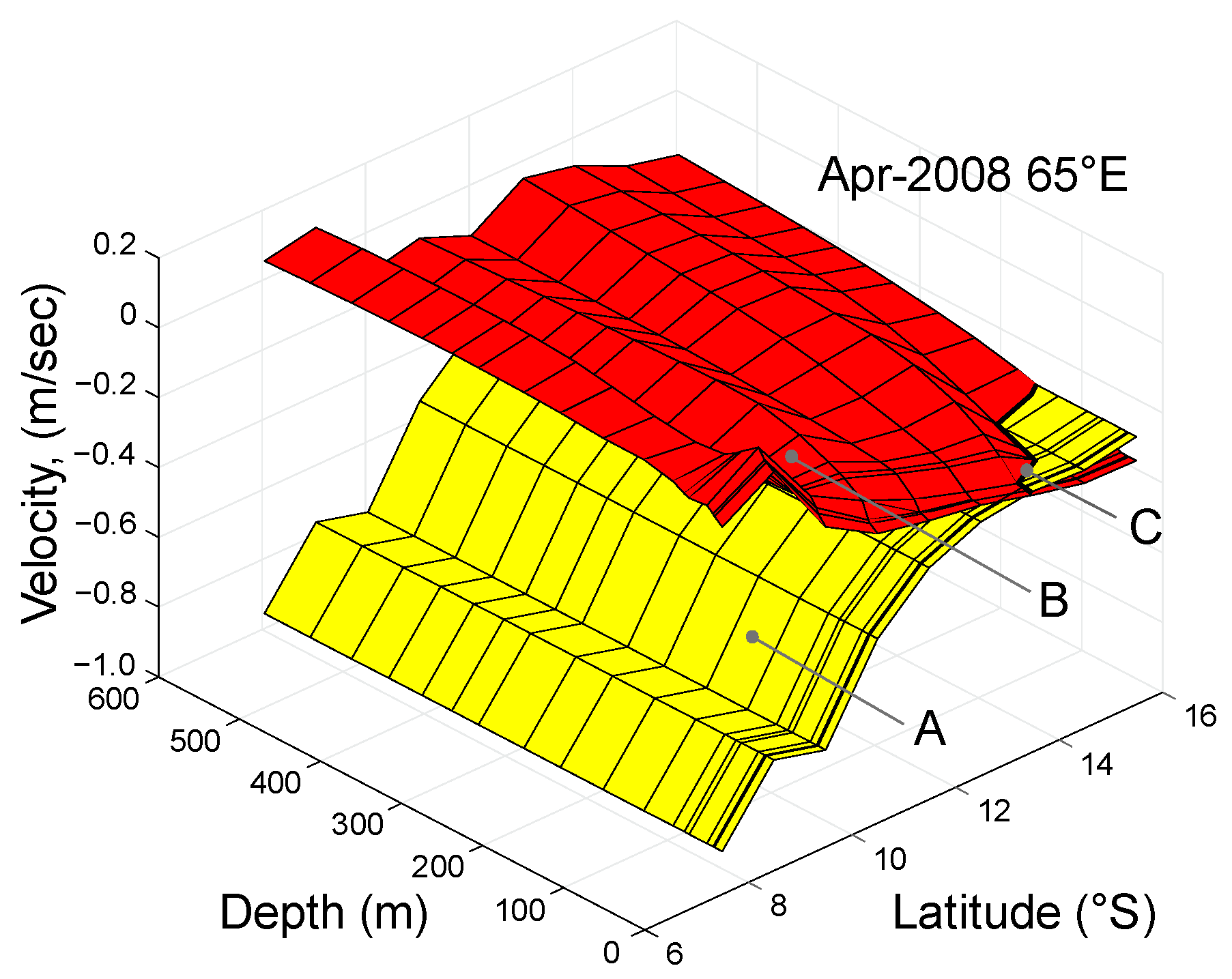
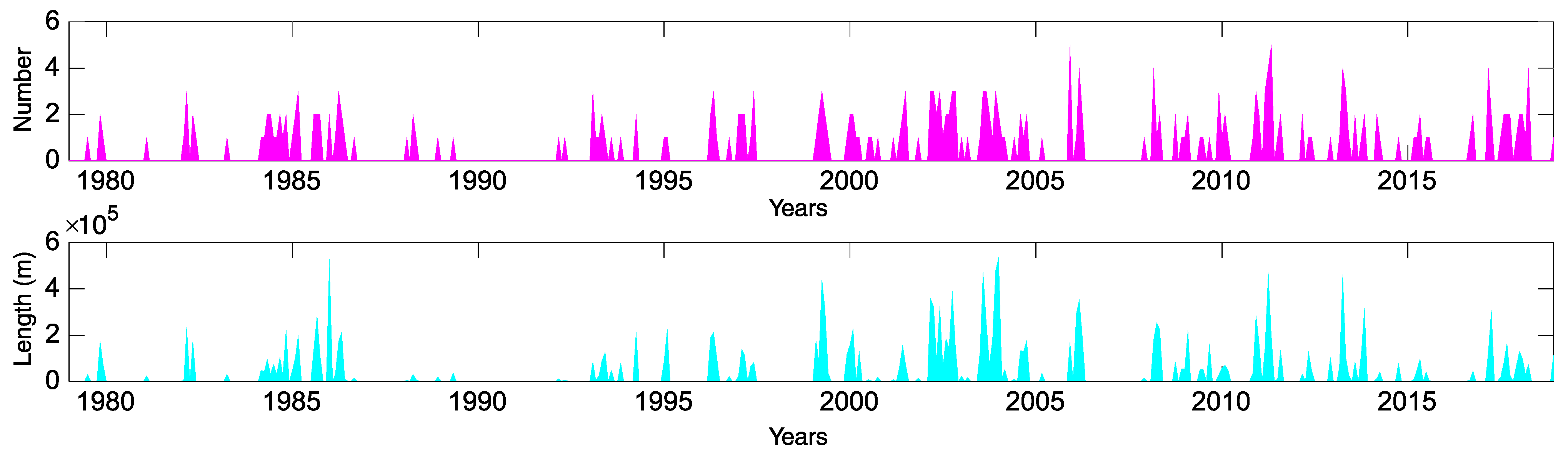
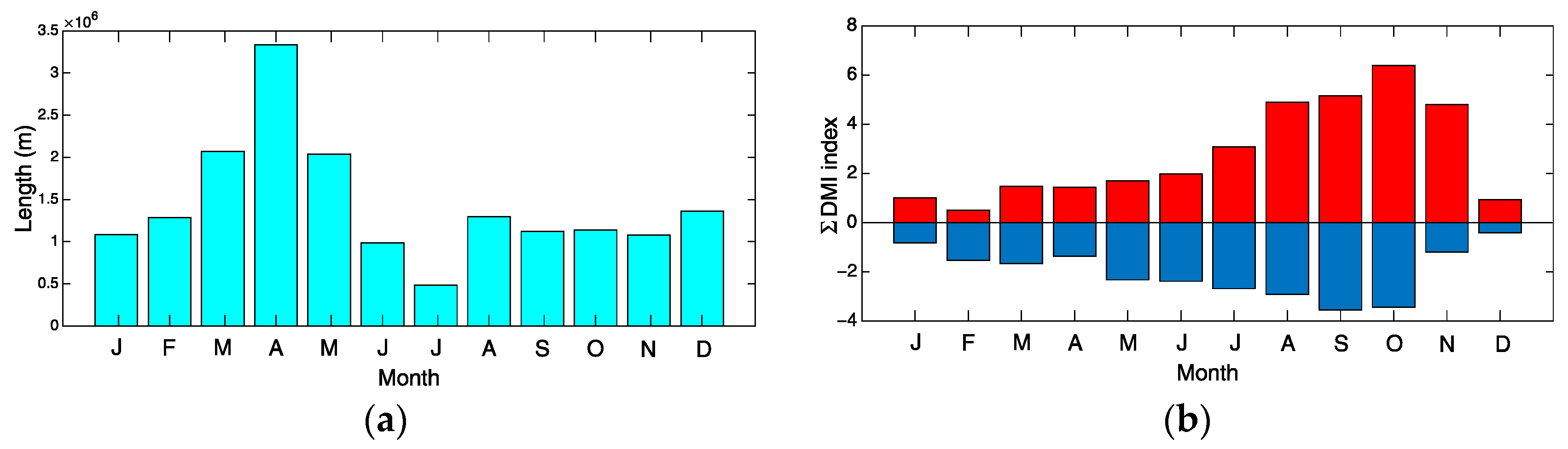
3.1. Critical Layers and IOD

Figure 4 shows the distribution of the total length of critical layers and sum of DMI index (for the IOD events with index more than 0.4) for each month for the period 1979–2018. It can be seen that this length is at a maximum in spring, especially in April. In other words, the total length of critical layers usually precedes the IOD event onset by one to two months.

Table 1. Years of positive and negative IOD events and the total length of the critical layers for each IOD event. The case of negative phase in 1998 (without critical layers) is shown in bold.

IOD Phase	Year	Critical Layer Length (km)	Summary Critical Layer Length (km)	Average Critical Layer Length (km)
Negative	1981	22.4
	1989	36.1
	1992	8.1
	1996	526.7
	1998	0	1427.3	158.9
	2005	204.0
	2010	459.4
	2014	121.7
	2016	48.75
	1982	410.9
	1983	30.4
	1994	210.4
Positive	1997	363.4	2831.9	353.9
	2006	602.3
	2012	293.6
	2015	176.3
	2017	744.1

shows that with the same number of events having different signs, the total length of the critical layers for positive events is almost twice as large as for negative events (2832 km vs. 1427 km). The IOD event of 1998 can be ignored, since this year there were no cases of the formation of a critical layer at all. The average value of the length of the critical layers is also approximately twice as large for positive events as for negative ones (354 km vs. 159 km). This suggests that the critical layers are formed two times more frequently during the years of a positive event IOD. Based on this, it can be assumed that the instability generated in the critical layer vicinity is the cause of the asymmetry of the amplitude of the DMI, which, as it is known, for positive events is on average greater than for negative ones. It should be noted that in some years of negative IOD events (for example, in 1996 and 2010) quite extended critical layers with a large total length are also observed. It may indicate that the presence of an extended critical layer at the beginning of the negative phase of the dipole can also impact its amplitude.

Figure 5 shows only positive DMI values and the total length of the critical layers in the years of positive quite strong IOD events. It can be seen that in all cases the most extended critical layers occurred at the beginning of a positive IOD event or a few months before (e.g., in 2006). It confirms that the instability of the zonal currents’ system can be one of the IOD generation causes. The varied delay between the month of formation of the extended critical layers and time of significant DMI rise can be explained by the following cause. Figure 4 and Figure 5 demonstrate the total length of the critical layers within the band shown in Figure 1. Certainly, the delay between the time of growing wave modes’ generation and the time of their manifestation in SST anomalies in the western and eastern parts of the equatorial–tropical Indian Ocean depends on the place of initial instability of the zonal currents’ system.

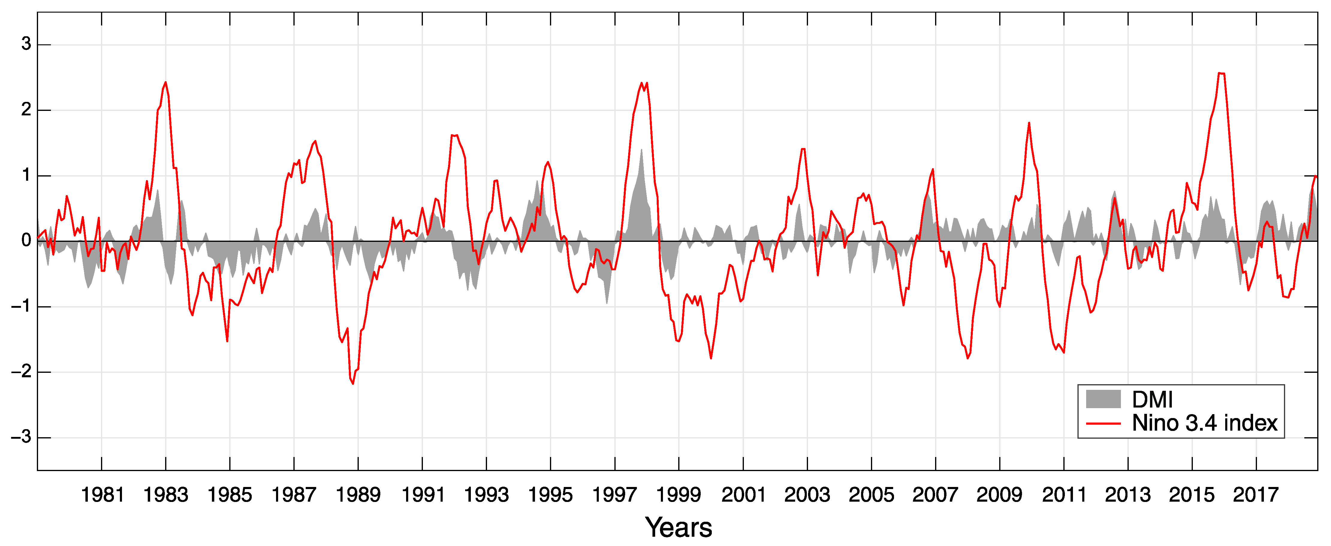
3.2. IOD–ENSO Interaction and Critical Layers

During the analysis of the IOD and ENSO time series for the period 1979–2018 (Figure 6), we came to the conclusion that the first type of IOD, which is usually described as part of the joint ENSO–IOD system (see Introduction), should be divided into two subtypes characterizing the IOD events by the start time of this event in relation to the nearest (in time) ENSO event. Therefore, in the further discussion, we discuss not two, but three IOD types. The first type is IOD events that occur after ENSO events and is most likely the result of the ENSO impact. The second IOD type represents the events that occur before the ENSO onset and are possibly the cause of its appearance. The third type is IOD events developing independently of the El Niño events and occur during the La Niña.

The IOD of 1998 can be attributed to the first IOD type, when the IOD event develops with a delay relative to ENSO one. In July 1998, the IOD went into a negative phase a month later than the ENSO, whose index took a negative value in June (Figure 7). It should be noted that the critical layers were absent in the southern part of the equatorial-tropical Indian Ocean throughout the year and the wave energy propagating from the Pacific Ocean during this period was not absorbed by the Indian Ocean zonal currents’ system. Thus, the neutral Rossby waves generated by the ENSO event can give rise to the development of the IOD event.

The second type, when the IOD event begins earlier than the El Niño one is well illustrated by the time series of DMI and Niño 3.4 index for 1994 (Figure 8). In this case, the DMI took a positive value of 0.3 already in March 1994, while ENSO was still in a negative phase. In April, when the Niño 3.4 index crossed zero, the DMI already had a significant positive value (0.4), which usually characterizes a strong IOD event. It should be noted that critical layers with a large length appear in this month. Therefore, the instability in the vicinity of these layers can be the cause of an increased DMI magnitude.

A striking manifestation of IOD in 1997–1998 can also be attributed to this type (Figure 9). This time, the IOD and ENSO, being in a positive phase, reached the maximum value for the entire period 1978–2018. In some previously published works (e.g., [39]), it is believed that IOD-1998 entered a positive phase simultaneously with ENSO. The presence of simultaneous variations in the IOD and ENSO indices time series explains the high level of correlation between IOD and ENSO events [40]; earlier it was often interpreted as proof of the leading role of ENSO in the development of IOD. This contradicts the fact that IOD entered a positive phase earlier than ENSO: in February 1997, the DMI took a positive value of 0.1 and did not change sign until July 1998, while the Niño 3.4 index passed into a positive phase only in April 1997. This suggests that the positive phase of IOD began earlier than El Niño. Therefore, this type of IOD event can provoke the generation of the ENSO events in the Pacific Ocean.

The fact that the IOD may not depend on the ENSO is also indicated by a comparison of the amplitudes of the IOD and ENSO of 1997 with similar events in 1982 and 2015 years (Figure 6). It can be seen that the IOD events’ intensity do not directly depend on the ENSO amplitude. The IOD event with a large amplitude in 1997 year, which occurred at about the same time as a very strong El Niño, is the exact opposite of the IOD events in 1982 and 2015 years, when the high-magnitude El Niño occurred but the amplitude of the IOD was significantly less. This suggests that IOD can be independent of the Pacific mode and arise due to the variations of the currents’ system in the Indian Ocean. This conclusion is confirmed by the presence of critical layers before and during the development of the positive IOD phase (Figure 5).

The third type of IOD events, acting in the El Niño absence, can be seen in the example of 2017 year (Figure 10). This Figure clearly shows that IOD events can be generated by the instability of the zonal currents of the Indian Ocean without any visible relation with the El Niño events. In fact, there were most extended critical layers for the entire considered period in the vicinity of the SEC in the Indian Ocean in this case (Table 1), and this confirms the above speculation. Note that development of this IOD event was accompanied by the La Niña event in the Pacific Ocean (Figure 10) and it is similar to the results of the scientific report [41].

4. Conclusions

Thus, it turns out that according to the ORAS5 re-analysis data, critical layers, in which the phase velocity of Rossby waves is equal to the average velocity of zonal currents, arise twice as often and with a greater length during the years of the positive IOD events. Most often, extended critical layers are formed in spring, one to two months before the IOD event onset. Hence, it follows that the presence of instability of the system of zonal currents, which probably develops in the vicinity of the critical layer before the IOD event, can be the reason for the generation of the IOD as an internal Indo-Ocean mode. This instability can also contribute to asymmetry in the amplitude of the dipole mode index between positive and negative IOD events.

It is shown that if an intense El Niño event is not accompanied by the formation of a critical layer, then IOD event develops with a slight delay relative to the positive ENSO phase. This proves that the neutral Rossby waves generated at the Eastern Indian Ocean edge spread westward and cause a response in the Indian Ocean in the form of IOD. In addition, it is demonstrated that the formation of an extended critical layer is possibly the cause of the appearance of an IOD event that does not depend on El Niño. Moreover, it can be accompanied by a La Niña event.

References

1. Saji, N.H.; Goswami, B.N.; Vinayachandran, P.N. A dipole mode in the tropical Indian Ocean. Nature 1999, 401, 360–363. [Google Scholar] [CrossRef] [PubMed]
2. Guo, F.; Qinyu, L.; Yang, J.; Fan, L. Three types of Indian Ocean Basin modes. Clim. Dyn. 2018, 51, 4357–4370. [Google Scholar] [CrossRef]
3. Saji, N.H.; Yamagata, T. Structure of SST and Surface Wind Variability during Indian Ocean Dipole Mode Events: COADS Observations. J. Clim. 2003, 16, 2735–2751. [Google Scholar] [CrossRef]
4. Rao, S.A.; Behera, S.K. Subsurface influence on SST in the tropical Indian Ocean: Structure and Interannual variability. Dyn. Atmos. Ocean. 2005, 39, 103–135. [Google Scholar] [CrossRef]
5. Birkett, C.; Murtugudde, R.; Allan, T. Indian Ocean climate event brings floods to East Africa’s lakes and the Sudd Marsh. Geophys. Res. Lett. 1999, 26, 1031–1034. [Google Scholar] [CrossRef]
6. Conway, D. Extreme rainfall events and lake level changes in East Africa: Recent events and historical precedents. East Afr. Great Lakes Limnol. Palaeolimnol. Biodivers. 2002, 12, 63–92. [Google Scholar]
7. Conway, D.; Allison, E.H.; Felstead, R. Rainfall variability in East Africa: Implications for natural resources management and livelihoods. Philos. Trans. R. Soc. A Math. Phys. Eng. Sci. 2005, 363, 49–54. [Google Scholar] [CrossRef]
8. Hashizume, M.; Chaves, L.F.; Minakawa, N. Indian Ocean Dipole drives malaria resurgence in East African highlands. Sci. Rep. 2012, 2, 269. [Google Scholar] [CrossRef] [Green Version]
9. Page, S.E.; Siegert, F.; Rieley, J. The amount of carbon released from peat and forest fires in Indonesia during 1997. Nature 2002, 420, 61–65. [Google Scholar] [CrossRef]
10. Kunii, O.; Kanagawa, S.; Yajima, I. The 1997 haze disaster in Indonesia: Its air quality and health effects. Arch. Environ. Health Int. J. 2002, 57, 16–22. [Google Scholar] [CrossRef]
11. Ummenhofer, C.C.; England, M.H.; Meyers, G.M. What causes southeast Australia’s worst droughts? Geophys. Res. Lett. 2009, 36, 1–5. [Google Scholar] [CrossRef] [Green Version]
12. Wang, G.; Cai, W. Two-year consecutive concurrences of positive Indian Ocean Dipole and Central Pacific El Niño preconditioned the 2019/2020 Australian “black summer” bushfires. Geosci. Lett. 2020, 7, 19. [Google Scholar] [CrossRef]
13. Wainwright, C.M.; Finney, D.L.; Kilavi, M. Extreme rainfall in East Africa, October 2019–January 2020 and context under future climate change. Weather 2021, 76, 26–31. [Google Scholar] [CrossRef]
14. Polonsky, A.B.; Torbinsky, A.V. Influence of the Indian ocean dipole on Danube summer drains. MSOE 2018, 34, 89–94. [Google Scholar] [CrossRef]
15. Polonsky, A.B. Response in the fields of surface air temperature, pressure and precipitation of the Eurasian region to the anomalies of ocean surface temperature associated with the Indian Ocean dipole. MSOE 2018, 31, 11–31. [Google Scholar]
16. Abram, N.J.; Wright, N.M.; Ellis, B. Coupling of Indo-Pacific climate variability over the last millennium. Nature 2020, 579, 385–392. [Google Scholar] [CrossRef]
17. Guo, F.; Liu, Q.; Sun, S. Three Types of Indian Ocean Dipoles. J. Clim. 2015, 28, 3073–3092. [Google Scholar] [CrossRef]
18. Ummenhofer, C.C.; Biastoch, A.; Claus, W. Multidecadal Indian Ocean variability linked to the Pacific and implications for preconditioning Indian Ocean dipole events. J. Clim. 2017, 30, 1739–1751. [Google Scholar] [CrossRef] [Green Version]
19. Saji, N.H.; Dachao, J.; Vishu, T. A model for super El Niños. Nat. Commun. 2018, 9, 2528. [Google Scholar]
20. Cretat, J.; Terray, P.; Masson, S. Indian Ocean and Indian summer monsoon: Relationships without ENSO in ocean–atmosphere coupled simulations. Clim. Dyn. 2017, 49, 1429–1448. [Google Scholar] [CrossRef]
21. Le, T.; Ha, K.J.; Bae, D.H. Causal effects of Indian Ocean Dipole on El Niño–Southern oscillation during 1950–2014 based on high-resolution models and reanalysis data. Environ. Res. Lett. 2020, 15, 385–392. [Google Scholar] [CrossRef]
22. Iizuka, S.; Matsuura, T.; Yamagata, T. The Indian Ocean SST dipole simulated in a coupled general circulation model. Geophys. Res. Lett. 2000, 27, 3369–3372. [Google Scholar] [CrossRef] [Green Version]
23. Vinayachandran, P.N.; Lizuka, S.; Yamagata, T. Indian Ocean dipole mode events in an ocean general circulation model. Deep Sea Res. Part II 2002, 49, 1573–1596. [Google Scholar] [CrossRef]
24. Cai, W.; Cowan, T.; Raupach, M. Positive Indian Ocean dipole events precondition southeast Australia bushfires. Geophys. Res. Lett. 2009, 36, 1–6. [Google Scholar] [CrossRef]
25. Allan, R. Is there an Indian Ocean dipole, and is it independent of the El Niño–Southern Oscillation? Clivar Exch. 2002, 6, 18–22. [Google Scholar]
26. Saji, N.H.; Xie, S.-P.; Yamagata, T. Tropical Indian Ocean variability in the IPCC twentieth-century climate simulations. J. Clim. 2006, 19, 4397–4417. [Google Scholar] [CrossRef] [Green Version]
27. Wang, H.; Murtugudde, R.; Kumar, A. Evolution of Indian Ocean dipole and its forcing mechanisms in the absence of ENSO. Clim. Dyn. 2016, 47, 2481–2500. [Google Scholar] [CrossRef]
28. Yoo, J.-H.; Moon, S.; Ha, K.-J.; Yun, K.-S.; Lee, J.-Y. Cases for the sole effect of the Indian Ocean Dipole in the rapid phase transition of the El Niño–Southern Oscillation. Theor. Appl. Climatol. 2020, 141, 999–1007. [Google Scholar] [CrossRef]
29. Philander, S.G. El Niño, La Nina, and the Southern Oscillation; Academic Press: San Diego, CA, USA, 1989; 293p. [Google Scholar]
30. Polonsky, A.B.; Torbinsky, A.V. Critical layer in equatorial-tropical zone and Indian Ocean dipole. MSOE 2019, 36, 88–93. [Google Scholar] [CrossRef]
31. Polonsky, A.B.; Torbinsky, A.V.; Gubarev, A.V. Identification of formation mechanisms of Indian Ocean dipole. MSOE 2020, 40, 13–19. [Google Scholar]
32. Chu, J.-E.; Ha, K.-J.; Lee, J.-Y.; Wang, B.; Kim, B.-H.; Chung, C.E. Future change of the Indian Ocean basin-wide and dipole modes in the CMIP5. Clim. Dyn. 2014, 43, 535–551. [Google Scholar] [CrossRef] [Green Version]
33. Polonsky, A.B.; Torbinsky, A.V. Velocity of propagation of temperature anomalies in the tropical zone of the Indian Ocean. Phys. Oceanogr. 2009, 63, 63–71. [Google Scholar] [CrossRef]
34. Polonsky, A.B.; Meyers, G.; Torbinsky, A.V. Interannual variability of the heat content of the upper layer in the equatorial Indian Ocean and the Indian-Ocean dipole. Phys. Oceanogr. 2007, 17, 129–140. [Google Scholar] [CrossRef]
35. Rao, S.A.; Behera, S.K.; Masumoto, Y. Interannual variability in the subsurface Indian Ocean with a special emphasis on the Indian Ocean Dipole. Deep Sea Res. Part II 2002, 49, 1549–1572. [Google Scholar] [CrossRef]
36. Bracco, A.; Kucharski, F.; Molteni, F.; Hazeleger, W.; Severijns, C. Internal and forced modes of variability in the Indian Ocean. Geophys. Res. Lett. 2005, 32, 1–4. [Google Scholar] [CrossRef] [Green Version]
37. Bubnov, V.A. Circulation in the Equatorial Zone of the World Ocean; Hydrometeoizdat: Leningrad, Russia, 1990. [Google Scholar]
38. Polonsky, A.B.; Torbinsky, A.V.; Gubarev, A.V. Verification of reanalysis data for the tropical zone of the Indian Ocean. Part 2. Characteristics of the averaged seasonal cycle and interannual variability. MSOE 2020, 42, 119–127. [Google Scholar] [CrossRef]
39. Saji, N.H. The Indian Ocean Dipole. Oxf. Res. Encycl. Clim. Sci. 2018, 46. [Google Scholar] [CrossRef]
40. Yamagata, T.; Behera, S.K.; Luo, J.J. Coupled ocean-atmosphere variability in the tropical Indian Ocean. E Earth’s Clim. Ocean.-Atmos. Interact. 2004, 147, 189–211. [Google Scholar]
41. Lim, E.-P.; Hendon, H.H. Causes and Predictability of the Negative Indian Ocean Dipole and Its Impact on La Niña During 2016. Sci. Rep. 2017, 7, 12619. [Google Scholar] [CrossRef] [PubMed] [Green Version]
Figure 1. Orientation map: area with coordinates of 7.5–15.5° S, 50–100° E in the Indian Ocean where the re-analysis ORAS5 data for potential temperature, salinity, and the zonal component of the current velocity were used.
Atmosphere 12 01662 g001
Figure 2. The distribution of the velocities of the zonal currents (B) and phase velocities of the first baroclinic mode of Rossby waves (A) by depth and latitude in April 2008 on a meridional section along 65° E. The critical layer is indicated by curve C. A sign “minus” indicates the spread of disturbances to the west.
Atmosphere 12 01662 g002
Figure 3. Time series of the number of critical layers per month (magenta) and the total length of critical layers per month (cyan) for the area with coordinates 7.5–15.5° S and 50–100° E for the period 1979–2018.
Atmosphere 12 01662 g003
Figure 4. Monthly distributions for the period 1979–2018: (a) cyan columns: total length of the critical layers, unit 106 m; (b) sum of DMI index (for the IOD events with index more than 0.4); red columns: positive IOD phase; blue columns: negative IOD phase).
Atmosphere 12 01662 g004
Figure 5. Histogram of DMI values in the years of the IOD positive phase and the total length of the critical layers (red columns: positive DMI; cyan columns: total length of the critical layers, unit 105 m. (a) 1982, (b) 1983, (c) 1994, (d) 1997, (e) 2006, (f) 2012, (g) 2015, (h) 2017).
Atmosphere 12 01662 g005
Figure 6. The dipole mode index (DMI) and index Niño 3.4 for the period 1978–2018.
Atmosphere 12 01662 g006
Figure 7. The dipole mode index (DMI) and Niño 3.4 index for the period December 1997–January 1999 (black curve and grey area: DMI; red curve: Niño 3.4 index).
Atmosphere 12 01662 g007
Figure 8. The dipole mode index (DMI), Niño 3.4 index and the total length of the critical layers for period July 1993–July 1995 (black curve and grey area: DMI; red curve: Niño 3.4 index; cyan columns: total length of the critical layer, unit 105 m).
Atmosphere 12 01662 g008
Figure 9. The dipole mode index (DMI), Niño 3.4 index and the total length of the critical layers for period December 1996–June 1998 (black curve and grey area: DMI; red curve: Niño 3.4 index; cyan columns: total length of the critical layer, unit 105 m).
Atmosphere 12 01662 g009
Figure 10. The dipole mode index (DMI), Niño 3.4 index and the total length of the critical layers for period June 2017–July 2018 (black curve and grey area: DMI; red curve: Niño 3.4 index; cyan columns: total length of the critical layer, unit 105 m).
Atmosphere 12 01662 g010